INLA: Integrated Nested Laplace Approximations · Integrated Nested Laplace Approximation (INLA) I One possible solution is INLA I The idea: for certain types of models, we can break

INLA: Integrated Nested Laplace Approximations

John Paige

Statistics DepartmentUniversity of Washington

October 10, 2017

1

The problem

I Markov Chain Monte Carlo (MCMC) takes too long in manysettings. How can we get a good approximation fast?

2

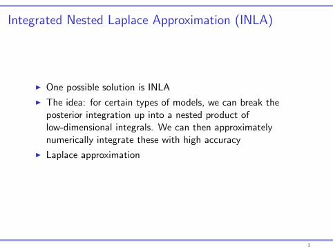
Integrated Nested Laplace Approximation (INLA)

I One possible solution is INLA

I The idea: for certain types of models, we can break theposterior integration up into a nested product oflow-dimensional integrals. We can then approximatelynumerically integrate these with high accuracy

I Laplace approximation

3

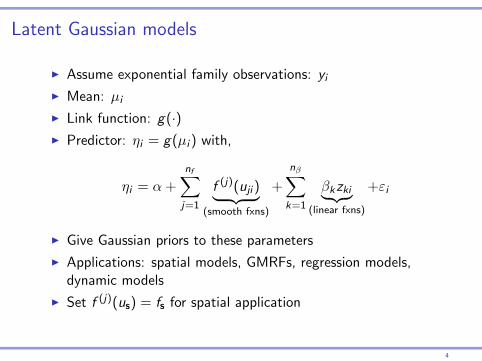
Latent Gaussian models

I Assume exponential family observations: yiI Mean: µiI Link function: g(·)I Predictor: ηi = g(µi ) with,

ηi = α +

nf∑j=1

f (j)(uji )︸︷︷︸(smooth fxns)

+

nβ∑k=1

βkzki︸︷︷︸(linear fxns)

+εi

I Give Gaussian priors to these parameters

I Applications: spatial models, GMRFs, regression models,dynamic models

I Set f (j)(us) = fs for spatial application

4

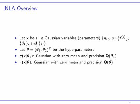
INLA Overview

I Let x be all n Gaussian variables (parameters) {ηi}, α,{f (j)}

,{βk}, and {εi}

I Let θ = (θ1,θ2)T be the hyperparameters

I π(x|θ1): Gaussian with zero mean and precision Q(θ1)

I π(x|θ): Gaussian with zero mean and precision Q(θ)

5

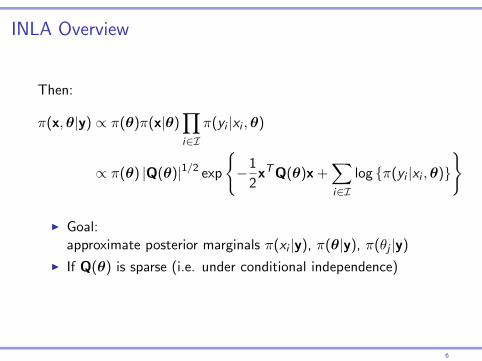
INLA Overview

Then:

π(x,θ|y) ∝ π(θ)π(x|θ)∏i∈I

π(yi |xi ,θ)

∝ π(θ) |Q(θ)|1/2 exp

{−1

2xTQ(θ)x +

∑i∈I

log {π(yi |xi ,θ)}

}

I Goal:approximate posterior marginals π(xi |y), π(θ|y), π(θj |y)

I If Q(θ) is sparse (i.e. under conditional independence)

6

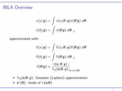
INLA Overview

π(xi |y) =

∫π(xi |θ, y)π(θ|y) dθ

π(θj |y) =

∫π(θ|y) dθ−j

approximated with:

π̃(xi |y) =

∫π̃(xi |θ, y)π̃(θ|y) dθ

π̃(θj |y) =

∫π̃(θ|y) dθ−j

π̃(θ|y) ∝ π(x,θ, y)

π̃G (x|θ, y)

∣∣∣∣x=x∗(θ)

I π̃G (x|θ, y): Gaussian (Laplace) approximationI x∗(θ): mode of π(x|θ)

7

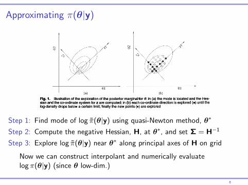
Approximating π(θ|y)

328 H. Rue, S. Martino and N. Chopin

second derivatives of log{7r(0|y)} by using the difference between successive gradient vectors. The gradient is approximated by using finite differences. Let 0* be the modal configuration.

(b) Step 2: at the modal configuration 0* compute the negative Hessian matrix H > 0, using finite differences. Let S = H-1, which would be the covariance matrix for 0 if the density were Gaussian. To aid the exploration, use standardized variables z instead of 0. Let £ = VAVT be the eigendecomposition of £, and define 0 via z, as follows:

0(z) = 0*+VA1/2z.

If n (0|y) is a Gaussian density, then z is jV(0, 1). This reparameterization corrects for.scale and rotation, and simplifies numerical integration; see for example Smith et al (1987).

(c) Step 3: explore log{7r(0|y)} by using the z-parameterization. Fig. 1 illustrates the procedure when log{7?(0|y)} is unimodal. Fig. l(a) shows a contour plot of log{7r(0|y)} for m = 2, the location of the mode and the mew co-ordinate axis for z. We want to explore log{7r(0|y)} to locate the bulk of the probability mass. The result of this procedure is displayed in Fig. l(b). Each dot is a point where log{7r(0|y)} is considered as significant, and which is used in the numerical integration (5). Details are as follows. We start from the mode (z = 0) and go in the positive direction of z\ with step length 6Z say Sz = 1, as long as

log[7r{0(O|y}] - log[7r{0(z)|y}] <6n (11)

where, for example, 6n = 2.5. Then we switch direction and do similarly. The other co- ordinates are treated in the same way. This produces the black dots. We can now fill in all the intermediate values by taking all different combinations of the black dots. These

new points (which are shown as gjey dots) are included if condition (11) holds. Since we lay out the points 0* in a regular grid, we may take all the area weights A* in equation (5) to be equal.

(d) Approximating 7r(0j\y): posterior marginals for 0j can be obtained directly from 7f(0|y) by using numerical integration. However, this is computationally demanding, as we need to evaluate 7f(0|y) for a large number of configurations. A more feasible approach is to use the points that were already computed during steps 1-3 to construct an interpolant

Fig. 1. Illustration of the exploration of the posterior marginal «for 0: in (a) the mode is located and the Hes- sian and the co-ordinate system for z are computed; in (b) each co-ordinate direction is explored (•) until the log-density drops below a certain limit; finally the new points (•) are explored

This content downloaded from 173.250.255.204 on Mon, 09 Oct 2017 16:29:31 UTCAll use subject to http://about.jstor.org/terms

Step 1: Find mode of log π̃(θ|y) using quasi-Newton method, θ∗

Step 2: Compute the negative Hessian, H, at θ∗, and set Σ = H−1

Step 3: Explore log π̃(θ|y) near θ∗ along principal axes of H on grid

Now we can construct interpolant and numerically evaluatelog π(θ|y) (since θ low-dim.)

8

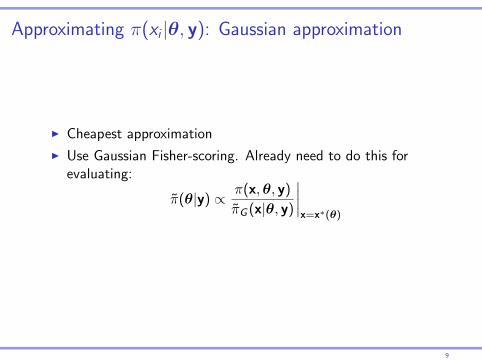
Approximating π(xi |θ, y): Gaussian approximation

I Cheapest approximation

I Use Gaussian Fisher-scoring. Already need to do this forevaluating:

π̃(θ|y) ∝ π(x,θ, y)

π̃G (x|θ, y)

∣∣∣∣x=x∗(θ)

9

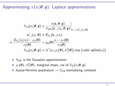
Approximating π(xi |θ, y): Laplace approximations

π̃LA(xi |θ, y) ∝ π(x,θ, y)

π̃GG (x−i |xi ,θ, y)

∣∣∣∣x−i=x∗−i (xi ,θ)

x∗−i (xi ,θ) ≈ Eπ̃G (x−i |xi )

⇒Eπ̃G (xj |xi )− µj(θ)

σj(θ)= aij(θ)

xi − µi (θ)

σi (θ)

π̃LA(xi |θ, y) ∝ N(xi ;µi (θ), σ2i (θ)

)exp {cubic spline(xi )}

I π̃GG is the Gaussian approximation

I µi (θ), σ2i (θ): marginal mean, var of π̃G (xi |θ, y)

I Gauss-Hermite quadrature → π̃LA normalizing constant

10

Approximating densities: Accuracy

I Accuracy depends on ‘effective number of parameters’ of x:

pD(θ) ≈ n − tr{

Q(θ)Q∗(θ)−1}

Low pD(θ)⇒ high accuracy

I For GMRF, asymptotic error rate is O(q/nd) for nd numberobservations, q rank of x Gaussian distribution

I In most cases, approximation errors cancel out reducing error

rates from O(n−1d ) to O(n−3/2d )

I These results apply to both approximations of π(x|θ, x) andof π(θ|y)

11

Approximating densities: Assessing errors

Idea 1:

π(θ|y)

π̃(θ|y)∝ Eπ̃G

[exp

{∑i

hi (xi )

}]

Where hi is log {π(yi |xi ,θ)} minus the second order term ofits Taylor expansion around x∗i (θ)

Idea 2: Compute symmetric Kullback Leibler divergence (SKLD) forGaussian, Laplace, and simplified Laplace approximations

12

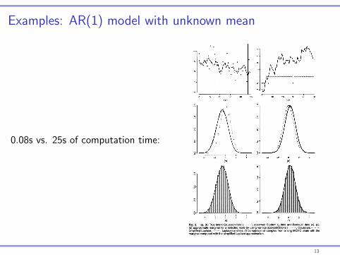
Examples: AR(1) model with unknown mean

0.08s vs. 25s of computation time:

Approximate Bayesian Inference for Latent Gaussian Models 335

Fig. 2. (a), (b) True latent Gaussian field (

(d) approximate marginal for a selected node by using various approximations (

simplified Laplace;

marginal computed with the simplified Laplace approximation


13

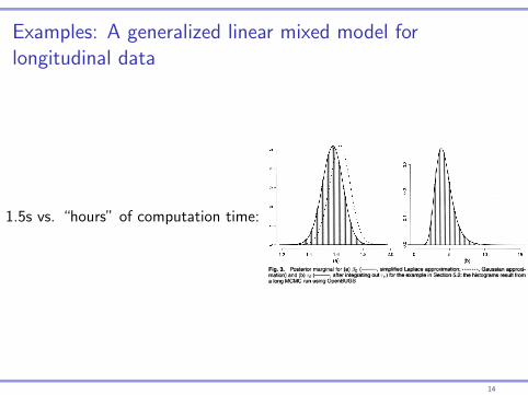
Examples: A generalized linear mixed model forlongitudinal data

1.5s vs. “hours” of computation time:


Fig. 3. Posterior marginal for (a) 0Q (

mation) and (b) re (

a long MCMC run using OpenBUGS

5. 3. Stochastic volatility models Stochastic volatility models are frequently used to analyse financial time series. Fig. 4(a) displays the logarithm of the «^ = 945 daily difference of the pound-dollar exchange rate from October 1st, 1981, to June 28th, 1985. This data set has been analysed by Durbin and Koopman (2000), among others. There has been much interest in developing efficient MCMC methods for such models, e.g. Shephard and Pitt (1997) and Chib et al. (2002).

The observations are taken to be

^I^^A/*{0, exp(r/,)}, t=l9...9nd. (26)

The linear predictor consists of two terms, rjt = // + /,, where ft is a first-order auto-regressive Gaussian process

/rl/l,...,/r-l,r,0-M0/r-l,l/r), |</>|< 1,

and ii is a Gaussian mean value. In this example, x = (/i, 771 , . . . , tjt)t and 0 = (0, r)T. The log- likelihood (with respect to rjt) is quite far from being Gaussian and is non-symmetric. There is some evidence that financial data have heavier tails than the Gaussian distribution, so a Student ^-distribution with unknown degrees of freedom can be substituted for the Gaussian distribution in expression (26); see Chib et al (2002). We consider this modified model at the end of this example.

We use the following priors: r~T(l, 0.1), </>'~AT(39l)9 where </>=2 exp(0')/{l+exp((//)}- 1, and /i ~ Af(0, 1 ) . We display the results for the Laplace approximation of the posterior marginals of the two hyperparameters and /i, but based on only the first 50 observations in Figs 4(b)-4(d), as using the full data set makes the approximation problem easier. The full curve in Fig. 4(d) is the marginal that was found by using simplified Laplace approximations and the broken curve uses Gaussian approximations, but in this case there are little differences (the SKLD is 0.05). The histograms are constructed from the output of a long MCMC run using OpenBUGS. The approximations that were computed are very precise and no deviance (in any node) can be detected. The results that were obtained by using the full data set are similar but the marginals are narrower (not shown).


14

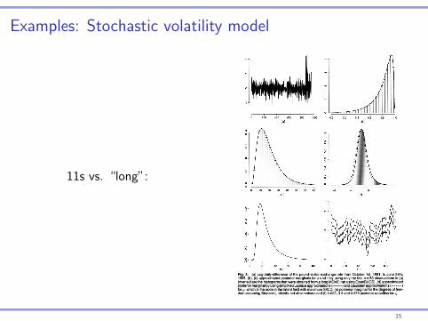
Examples: Stochastic volatility model

11s vs. “long”:


Fig. 4. (a) Log-daily-difference of the pound-dollar exchange rate from October 1st, 1981, to June 28th, 1985, (b), (c) approximated posterior marginals for <j> and r by using only the first n = 50 observations in (a) (overlaid are the histograms that were obtained from a long MCMC run using OpenBUGS), (d) approximated posterior marginal by using simplified Laplace approximations (

for //, which is the node in the latent field with maximum SKLD, (e) posterior marginal for the degrees of freedom assuming Student ^-distributed observations and (f) 0.025, 0.5 and 0.975 posterior quantiles for 77/


15

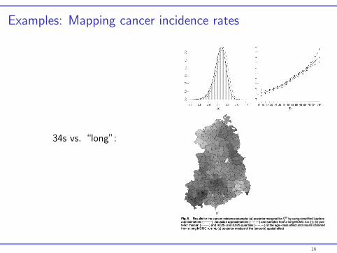
Examples: Mapping cancer incidence rates

34s vs. “long”:


Fig. 5. Results for the cancer incidence example: (a) posterior marginal for £p by using simplified Laplace approximations (

terior median (

from a long MCMC run (•); (c) posterior median of the (smooth) spatial effect

We start by dividing the area of interest into a 200 x 100 regular lattice, where each square pixel of the lattice represents 25 m2. This makes rid = 20000. The scaled and centred versions of the altitude and norm of the gradient are shown in Figs 6(b) and 6(c) respectively. For the spatial structured term, we use a second-order polynomial intrinsic GMRF (see Rue and Held (2005), section 3.4.2), with following full conditionals in the interior (with obvious notation)


16

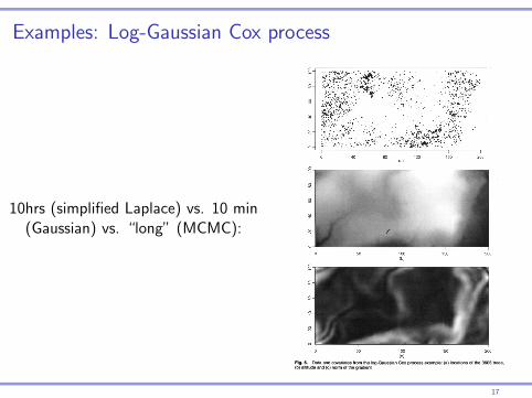
Examples: Log-Gaussian Cox process

10hrs (simplified Laplace) vs. 10 min(Gaussian) vs. “long” (MCMC):


Fig. 6. Data and covariates from the log-Gaussian Cox process example: (a) locations of the 3605 trees, (b) altitude and (c) norm of the gradient


17

Questions?

18

Documents

INLA: Integrated Nested Laplace Approximations · Integrated Nested Laplace Approximation (INLA) I One possible solution is INLA I The idea: for certain types of models, we can break