The R-INLA package

David BolinChalmers University of Technology

Búzios, RJ, Brazil,June 18, 2014

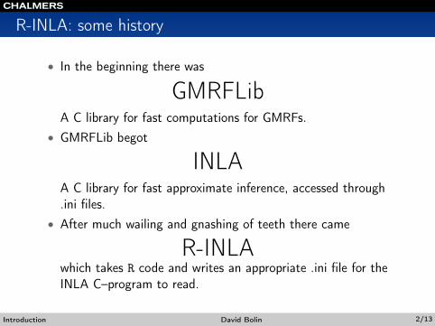
R-INLA: some history

• In the beginning there was

GMRFLibA C library for fast computations for GMRFs.

• GMRFLib begot

INLAA C library for fast approximate inference, accessed through.ini files.

• After much wailing and gnashing of teeth there came

R-INLAwhich takes R code and writes an appropriate .ini file for theINLA C–program to read.

Introduction David Bolin 2/13

Obtaining R-INLA

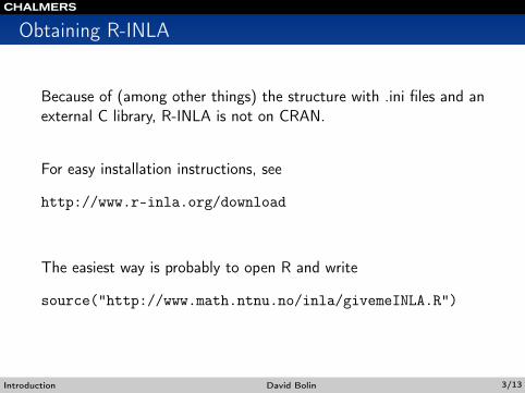
Because of (among other things) the structure with .ini files and anexternal C library, R-INLA is not on CRAN.

For easy installation instructions, see

http://www.r-inla.org/download

The easiest way is probably to open R and write

source("http://www.math.ntnu.no/inla/givemeINLA.R")

Introduction David Bolin 3/13

Bayesian structured additive regression models

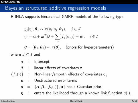
R-INLA supports hierarchical GMRF models of the following type:

yj |ηj ,θ1 ∼ π(yj |ηj ,θ1), j ∈ J

ηi = α+ ziTβ +

∑γ

fγ(cγ,i) + ui, i ∈ I

θ = (θ1,θ2) ∼ π(θ), (priors for hyperparameters)

where J ⊂ I and

α : Interceptβ : linear effects of covariates z

{fγ(·)} : Non-linear/smooth effects of covariates cγu : Unstructured error termsx = {α,β, {fγ(·)},u} has a Gaussian prior.η : enters the likelihood through a known link function g(·).

Introduction David Bolin 4/13

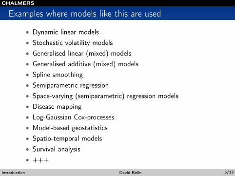
Examples where models like this are used

• Dynamic linear models• Stochastic volatility models• Generalised linear (mixed) models• Generalised additive (mixed) models• Spline smoothing• Semiparametric regression• Space-varying (semiparametric) regression models• Disease mapping• Log-Gaussian Cox-processes• Model-based geostatistics• Spatio-temporal models• Survival analysis• +++

Introduction David Bolin 5/13

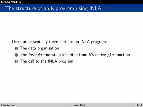
The structure of an R program using INLA

There are essentially three parts to an INLA program:1 The data organisation2 The formula—notation inherited from R’s native glm function3 The call to the INLA program.

Introduction David Bolin 6/13

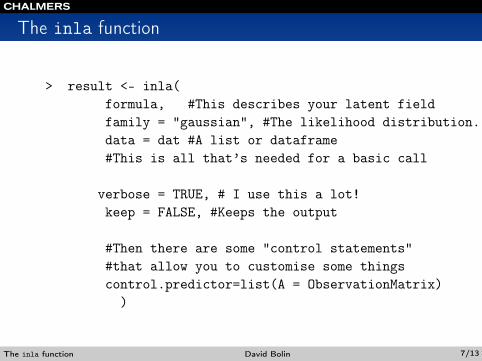
The inla function

> result <- inla(formula, #This describes your latent fieldfamily = "gaussian", #The likelihood distribution.data = dat #A list or dataframe#This is all that’s needed for a basic call

verbose = TRUE, # I use this a lot!keep = FALSE, #Keeps the output

#Then there are some "control statements"#that allow you to customise some thingscontrol.predictor=list(A = ObservationMatrix)

)

The inla function David Bolin 7/13

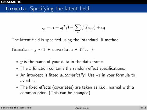
formula: Specifying the latent field

ηi = α+ ziTβ +

∑γ

fγ(cγ,i) + ui

The latent field is specified using the “standard” R method

formula = y ∼ 1 + covariate + f(...).

• y is the name of your data in the data frame.• The f function contains the random effect specifications.• An intercept is fitted automatically! Use -1 in your formula toavoid it.

• The fixed effects (covariates) are taken as i.i.d. normal with acommon prior. (This can be changed)

Specifying the latent field David Bolin 8/13

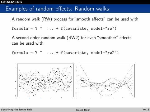
Examples of random effects: Random walks

A random walk (RW) process for “smooth effects” can be used with

formula = Y ~ ... + f(covariate, model="rw")

A second-order random walk (RW2) for even “smoother” effectscan be used with

formula = Y ~ ... + f(covariate, model="rw2")

Specifying the latent field David Bolin 9/13

SPDE models in INLA

The SPDE models have been incorporated into the INLA package.• This means that they work well with INLA!• But they also work outside of INLA

To specify an SPDE model we need to1 Create the mesh for the model.2 Construct the observation matrix that links the measurement

locations to the mesh locations.3 Create an spde object.

After this, the SPDE model is used like any other random effectmodel in the formula, using f(locations, model="spde")

Specifying SPDE models David Bolin 10/13

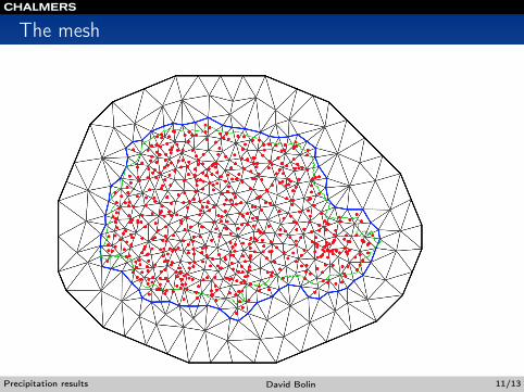
The mesh

Precipitation results David Bolin 11/13

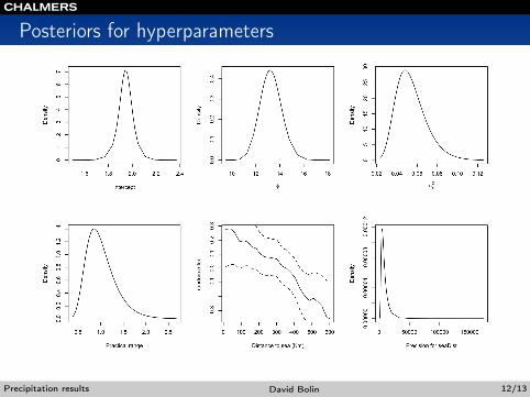
Posteriors for hyperparameters

Precipitation results David Bolin 12/13

Kriging results: Gamma (left) and Gaussian (right)

Precipitation results David Bolin 13/13