Bayesian Spatial Modelling with R-INLAinla.r-inla-download.org/r-inla.org/papers/jss/lindgren.pdf · 2 Bayesian Spatial Modelling with R-INLA is that classical Gaussian random elds

JSS Journal of Statistical SoftwareMMMMMM YYYY, Volume VV, Issue II. http://www.jstatsoft.org/

Bayesian Spatial Modelling with R-INLA

Finn LindgrenUniversity of Bath, United Kingdom

Havard RueNorwegian University of Science and Technology, Norway

Abstract

The principles behind the interface to continuous domain spatial models in the R-INLA software package for R are described. The Integrated Nested Laplace Approxima-tion (INLA) approach proposed by Rue, Martino, and Chopin (2009) is a computationallyeffective alternative to MCMC for Bayesian inference. INLA is designed for latent Gaus-sian models, a very wide and flexible class of models ranging from (generalized) linearmixed to spatial and spatio-temporal models. Combined with the Stochastic Partial Dif-ferential Equation approach (SPDE, Lindgren and Lindgren 2011), one can accommodateall kinds of geographically referenced data, including areal and geostatistical ones, as wellas spatial point process data. The implementation interface covers stationary spatial mod-els, non-stationary spatial models, and also spatio-temporal models, and is applicable inepidemiology, ecology, environmental risk assessment, as well as general geostatistics.

Keywords: Bayesian inference, Gaussian Markov random fields, stochastic partial differentialequations, Laplace approximation, R.

Traditionally, Markov models in image analysis and spatial statistics have been largely con-fined to discrete spatial domains, such as lattices and regional adjacency graphs. However,as discussed in Lindgren, Rue, and Lindstrom (2011), one can express a large class of ran-dom field models as solutions to continuous domain stochastic partial differential equations(SPDEs), and write down explicit links between the parameters of each SPDE and the ele-ments of precision matrices for weights in a discrete basis function representation. As shownby Whittle (1963), such models include those with Matern covariance functions, which areubiquitous in traditional spatial statistics, but in contrast to covariance based models it isfar easier to introduce non-stationarity into the SPDE models. This is because the differ-ential operators act locally, similarly to local increments in Gibbs-specifications of Markovmodels, and only mild regularity conditions are required. The practical significance of this

http://www.jstatsoft.org/

2 Bayesian Spatial Modelling with R-INLA

is that classical Gaussian random fields can be merged with methods based on the Markovproperty, providing continuous domain models that are computationally efficient, and wherethe parameters can be specified locally without having to worry about positive definitenessof covariance functions.

The fundamental building block of such Gaussian Markov random field (GMRF) models, asimplemented in R-INLA, is a high-dimensional basis representation, with simple local basisfunctions. This is in contrast to Fixed Rank Kriging (Cressie and Johannesson 2008) thattypically uses a smaller number of global basis functions, and predictive process methods(Banerjee, Gelfand, Finley, and Sang 2008). See Wikle (2010) of for an overview of suchlow-rank representation methods. A numerical comparison of the error introduced in Krigingcalculations was performed by Bolin and Lindgren (2013) for SPDE based GMRF models,covariance tapering, and process convolutions. A non-parametric approach using similarGMRF models is available in the LatticeKrig package in CRAN (Nychka, Hammerling, Sain,and Lenssen 2013).

The different methods can also be combined, although the details for doing that within R-INLA are beyond the scope of this paper. For example, the global temperature analysis inLindgren et al. (2011) used a combination of a low dimensional global basis, like in FixedRank Kriging, and a small-scale GMRF process, both with priors based on approximations tocontinuous domain SPDE models. There is considerable overlap between models formulatedusing Fixed Rank Kriging and SPDE/GMRF models, and a clear line separating the methodscannot be drawn.

The R-INLA software package currently has direct support for stationary and non-stationarylocally isotropic SPDE/GMRF models on compact subsets of R, R2, and on S2, as well asseparable space-time models. Some non-separable space-time models, non-stationary fullyanisotropic models, as well as models on R3 and other user-defined domains are also partiallysupported by the internal implementation, but have not yet been added to the basic interface.Consequently, auto-regressive models (see e.g., Cameletti, Lindgren, Simpson, and Rue 2013)are fully supported, but anisotropic advection-diffusion models (see e.g., Sigrist, Kunsch,and Stahel 2014) are limited to non-advective models and require advanced user interaction,but support non-stationary anisotropy if only the strength of the non-isotropic diffusion isunknown.

The following sections present the basic ingredients of the link between continuous domainsand Markov models and related simulation free Bayesian inference methods (Section 1), de-scribe the structure of the interface to using such models in the R-INLA software package(Section 2 and 3), and discuss planned future development (Section 4). Special emphasis isplaced on the abstractions necessary to simplify the practical bookkeeping for the users of thesoftware. For further details on the computational and inferential methods in the R-INLApackage we refer to Martins, Simpson, Lindgren, and Rue (2013).

1. Spatial modelling and inference

This section describes the basic principles of the continuous domain spatial models andBayesian inference methods in the R-INLA package (Rue, Martino, Lindgren, Simpson, andRiebler 2013b).

Journal of Statistical Software 3

1.1. Continuous domain spatial Markov random fields

When building and using hierarchical models with latent random fields it is important toremember that the latent fields often represent real-world phenomena that exist independentlyof whether they are observed in a given location or not. Thus, we are not building models solelyfor discretely observed data, but for approximations of entire processes defined on continuousdomains. For a spatial field x(s), while the data likelihood typically depends only on thevalues at a finite set of locations, s1, . . . , sm, the model itself defines the joint behaviourfor all locations, typically s ∈ R2 or s ∈ S2 (a sphere/globe). In the case of lattice data,the discretisation typically happens in the observation stage, such as integration over gridboxes (e.g., photon collection in a camera sensor). Often, this is approximated by point-wise evaluation, but there is nothing apart from computational challenges preventing otherobservation models.

As discussed in the introduction, an alternative to traditional covariance based modellingis to use SPDEs, but carry out the practical computations using Gaussian Markov randomfield (GMRF) representations. This is done by approximating the full set of spatial ran-dom functions with weighted sums of simple basis functions, which allows us to hold on tothe continuous interpretation of space, while the computational algorithms only see discretestructures with Markov properties. Beyond the main paper Lindgren et al. (2011), this isfurther discussed by Simpson, Lindgren, and Rue (2012a,b).

Stationary Matern fields

The simplest model for x(s) currently implemented in R-INLA is the SPDE/GMRF versionof the stationary Matern family, obtained as the stationary solutions to

(κ2 −∆)α/2(τx(s)) =W(s), s ∈ Ω,

where ∆ is the Laplacian, κ is the spatial scale parameter, α controls the smoothness of therealisations, τ controls the variance, and Ω is the spatial domain. The right-hand side of theequation, W(s), is a Gaussian spatial white noise process. As noted by Whittle (1954, 1963),the stationary solutions on Rd have Matern covariances,

COV(x(0), x(s)) =σ2

2ν−1Γ(ν)(κ‖s‖)ν Kν(κ‖s‖). (1)

The parameters in the two formulations are coupled so that the Matern smoothness is ν =α− d/2 and the marginal variance is

σ2 =Γ(ν)

Γ(α)(4π)d/2κ2ντ2. (2)

From this we can identify the exponential covariance with ν = 1/2. For d = 1, this is obtainedwith α = 1, and for d = 2 with α = 3/2.

From spectral theory one can show that integer values for α gives continuous domain Markovfields (Rozanov 1982), and these are the easiest for which to provide discrete basis represen-tations. In R-INLA, the default value is α = 2, but 0 ≤ α < 2 are also available, thoughnot as extensively tested. For the non-integer α values the approximation method introducedin the authors’ discussion response in Lindgren et al. (2011) is used. Historically, Whittle


(1954) argued that α = 2 was a more natural basic choice for d = 2 models than the frac-tional α = 3/2 alternative. Note that fields with α ≤ d/2 have ν ≤ 0 and that such fieldshave no point-wise interpretation, although they have well-defined integration properties. Inparticular, this means that the case d = 2, α = 1, which on a regular lattice discretisationcorresponds to the common CAR(1) model, needs to be interpreted with care (Besag 1981;Besag and Mondal 2005), especially when used in combination with irregular discretisationdomains.

The models discussed in Lindgren et al. (2011) and implemented in R-INLA are built on abasis representation

x(s) =

n∑k=1

ψk(s)xk, (3)

where ψk(·) are deterministic basis functions, and the joint distribution of the weight vectorx = x1, . . . , xn is chosen so that the distribution of the functions x(s) approximates thedistribution of solutions to the SPDE on the domain. To obtain a Markov structure, andto preserve it when conditioning on local observations, we use piecewise polynomial basisfunctions with compact support. The construction is done by projecting the SPDE onto thebasis representation in what is essentially a Finite Element method.

To allow easy and explicit evaluation, for two-dimensional domains we use piece-wise linearbasis functions defined by a triangulation of the domain of interest. For one-dimensionaldomains, B-splines of degrees 1 (piecewise linear) and 2 (piecewise quadratic) are supported.This yields sparse matrices C, G1, and G2 such that the appropriate precision matrix for theweights is given by

Q = τ2(κ4C + 2κ2G1 +G2)

for the default case α = 2, so that the elements of Q have explicit expressions as functionsof κ and τ . Assigning the Gaussian distribution x ∼ N(0,Q−1) now generates continuouslydefined functions x(s) that are approximative solutions to the SPDE (in a stochastically weaksense).

The simplest internal representation of the parameters in the model interface is log(τ) = θ1

and log(κ) = θ2, where θ1 and θ2 are assigned a joint normal prior distribution. Since τand κ have a joint influence on the marginal variances of the resulting field, it is often morenatural to construct the parameter model using the standard deviation σ and range ρ, whereρ = (8ν)1/2/κ is the distance for which the correlation functions have fallen to approximately0.13, for all ν > 1/2. Another commonly used definition for the range is as the distance atwhich the correlation is 0.05. The alternative definition used in R-INLA has the advantageof explicit dependence on ν. Translating this into τ and κ yields

log τ =1

2log

(Γ(ν)

Γ(α)(4π)d/2

)− log σ − ν log κ, (4)

log κ =log(8ν)

2− log ρ. (5)

Suppose we want a parameterisation

log σ = log σ0 + θ1, (6)

log ρ = log ρ0 + θ2, (7)


where σ0 and ρ0 are base-line standard deviation and range values. We then substitute log σand log ρ into Equation 4 and 5, giving the internal parameterisation

log κ0 =log(8ν)

2− log ρ0,

log τ0 =1

2log

(Γ(ν)

Γ(α)(4π)d/2

)− log σ0 − ν log κ0,

log τ = log τ0 − θ1 + νθ2,

log κ = log κ0 − θ2,

where now the θ1 and θ2 parameters jointly control the τ -parameter.

Non-stationary fields

There is a vast range of possible extensions to the stationary SPDE described in the previoussection, including non-stationary versions (see Lindgren et al. 2011; Bolin and Lindgren 2011,for examples). In the current version of the package, a non-stationary model defined viaspatially varying κ(s) and τ(s) is available for the case α = 2. The SPDE is defined as

(κ(s)2 −∆)(τ(s)x(s)) =W(s), s ∈ Ω,

and log κ(s) and log τ(s) are defined as linear combinations of basis functions,

log(τ(s)) = bτ0(s) +

p∑k=1

bτk(s)θk,

log(κ(s)) = bκ0(s) +

p∑k=1

bκk(s)θk,

where θ1, . . . , θp is a common set of internal representation parameters, and bτk(·) and bκk(·)are spatial basis functions, some of which, for each k may be identically zero for either τ orκ. The precision matrix for the discrete field representation weights is a simple modificationof the stationary one, with the parameter fields (evaluated at the mesh discretisation points)entering via diagonal matrices:

T = diag(τ(sk)),

K = diag(κ(sk)),

Q = T (K2CK2 +K2G1 +G>1 K2 +G2)T .

Just as in the stationary case, the model can be reparameterised using Equation 4 and 5,where

log(σ(s)) = bσ0 (s) +

p∑k=1

bσk(s)θk,

log(ρ(s)) = bρ0(s) +

p∑k=1

bρk(s)θk,


and σ(s) and ρ(s) are the nominal local standard deviations and correlation ranges. Thereare no explicit expressions for the actual values, since they depend on the entire parameterfunctions in a non-trivial way. For given values of θ, the marginal variances can be efficientlycalculated using the discretised GMRF representation, see Section 2.3.

Given the offsets, bσ0 (s) and bκ0(s), and basis functions. bσk(s) and bκk(s), for the log(σ(s))and log(ρ(s)) parameter fields, the internal model representation can be constructed usingthe following identities:

bκ0(s) =log(8ν)

2− bρ0(s), (8)

bκk(s) = −bρk(s), (9)

bτ0(s) =1

2log

(Γ(ν)

Γ(α)(4π)d/2

)− bσ0 (s)− νbκ0(s), (10)

bτk(s) = −bσk(s)− νbκk(s). (11)

The constant Γ(ν)/(Γ(α)(4π)d/2) is 1/2 and 1/4 for d = 1, α = 1 and 2. For d = 2 and α = 2it is 1/(4π). There is experimental support for constructing basis functions that reduces theinfluence of the range on the variance for cases where the basis functions for log ρ(s) haverapid changes.

Boundary effects

When constructing solutions to the SPDEs on bounded domains, boundary conditions areimposed, but how to construct practical and proper stochastic boundary conditions for thesemodels is an open research problem. In the current version of the package, all 2D models arerestricted to deterministic Neumann boundaries (zero normal-derivatives), as this is easy toconstruct, has well defined physical interpretation in terms of reflection, and has an effect onthe covariances that is easy to quantify. As a rule of thumb, the boundary effect is negligibleat a distance ρ from the boundary, and the variance is inflated near the boundary by a factor2 along straight boundaries, and by a factor 4 near right-angled corners. In practice one cantherefore avoid the boundary effect by extending the domain of interest by a distance at leastρ, as well as avoid sharp corners. The built-in mesh generation routines (see Section 2.1)are designed to do this. For one-dimensional models, the boundaries can also be defined asDirichlet (value zero at the boundary), free, or cyclic.

Space-time models

While no space-time models are currently implemented explicitly, it is possible to constructsuch models using general code features. The most important method is to construct aKronecker product model. Starting from a basis representation

x(s, t) =∑k

ψk(s, t)xk,

where each basis function is the product of a spatial and a temporal basis function, ψk(s, t) =ψsi (s)ψtj(t), the space-time SPDE

∂

∂t(κ(s)2 −∆)α/2 (τ(s)x(s, t)) =W(s, t), (s, t) ∈ Ω× R


generates a precision matrix for the weight vector x as Q = Qt ⊗ Qs, where Qs is theprecision for the previous purely spatial model, and Qt is the precision corresponding to aone-dimensional random walk. Any temporal GMRF model can be used in this construction,and Section 3 contains examples for how to specify such models in R-INLA. See Camelettiet al. (2013) for a case-study using a Kronecker-model based on a temporal AR(1) process,including the full R code (although note that the interface has evolved slightly since thecase-study was implemented).

Kronecker models generate separable covariance functions, which are simple but often unre-alistic. The internal representation of the SPDE precision structures however also permitsconstruction of non-separable models, as long as the unknown parameters appear in the ap-propriate places. Non-separable models that can be constructed in this way include specialcases of the stochastic heat equation. Wrapper functions for constructing such models areexpected to be added in the future, as well as extensions for advection-diffusion models.

1.2. Bayesian inference

The R-INLA package (Rue et al. 2013b) implements the Integrated Nested Laplace Approxi-mation (INLA) method introduced by Rue et al. (2009). This method performs direct numer-ical calculation of posterior densities in a large Latent Gaussian (LGM) sub-class of Bayesianhierarchical models, avoiding time-consuming Markov chain Monte Carlo simulations. Theimplementation covers models of the following form,

(θ) ∼ p(θ) (12)

(x | θ) ∼ N(0,Q(θ)−1) (13)

ηi =∑j

cijxj (14)

(yi | x,θ) ∼ p(yi | ηi,θ) (15)

θ are (hyper)parameters, x is a latent Gaussian field, η is a linear predictor based on knowncovariate values cij , and y is a data vector,

The basic principle is to approximate the posterior density for (θ | y) using a Gaussianapproximation p(x | θ, y) for the posterior for the latent field, evaluated at the posteriormode, x∗(θ) = argmax

xp(x | θ, y),

p(θ | y) ∝ p(θ, x, y)

p(x | θ, y)

∣∣∣∣x=x∗(θ)

≈ p(θ, x, y)

p(x | θ, y)

∣∣∣∣x=x∗(θ)

,

which is called a Laplace approximation. This allows approximate evaluation of the (unnor-malised) posterior density for θ at any point. The algorithm uses numerical optimisation tofind the mode of the posterior. The marginal posteriors for each θk and xj are then calculatedusing numerical integration over θ, with another Laplace approximation involved in the latentfield marginal posterior calculations:

p(θk | y) ≈∫p(θ | y) dθ−k,

p(xj | y) ≈∫p(xj | θ, y) p(θ | y) dθ


For more details and information, see Martins et al. (2013).

The linear predictor

An important aspect of the package interface is how to specify the connection between thelatent field x and the linear predictor η. R-INLA uses a formula syntax similar to the standardone used for linear model estimation with lm(). The main difference is that random effectsof all kinds, including smooth nonlinear effects, structured graph effects and spatial effects,are specified using terms f(), where the user specifies the properties of such effects. Thefirst argument of each f() specifies what element of the latent effect should apply to eachobservation, either as a scalar location of covariate value (for smooth nonlinear effects) or asa direct component index.

The linear predictor ηi = fixediβ + f(timei) + randomi can be constructed using the formula

~ -1 + fixed + f(time, model="rw2") + f(random, model="iid")

Let z(1) and z(2) denote the covariate values for the fixed and time effects, and let z(3)

denote random effect indices. We can then rewrite the linear model from Equation 14 usingmapping functions hk(·) that denote the mapping from covariates or indices to the actuallatent value for formula component k,

h1(z(1)i ) = z

(1)i β

h2(z(2)i ) = smooth effect evaluated at z

(2)i

h3(z(3)i ) = random effect component number z

(3)i

ηi =∑k

hk(z(k)i )

The latent field is the joint vector of all latent Gaussian variables, including the linear covariateeffect coefficient β. For missing values in the z-vectors, the h functions are defined to be zero.

Since this construction only allows each observation to directly depend on a single elementfrom each hk(·) effect, this does not cover the case when an effect is defined using a basisexpansion such as Equation 3. To solve this, R-INLA can apply a second layer of linearcombinations to the η predictor,

η∗ = Aη, (16)

where A is a user-defined sparse matrix. This allows the SPDE models to be treated asindexed random effects, and the mapping between the basis weights and function values isdone by placing appropriate ψj(s) values in the A matrix. Whenever an A matrix is used,the elements of the η∗ vector are the linear predictor values used in the general observationmodel in Equation 15, instead of η. This is further formalised in Section 2.5.

See Section 2.2 for how to construct the part of the A matrix needed for an SPDE model,and Section 2.5 for how to set up the joint matrices needed for general models.

2. R interface


The R-INLA interface to the SPDE models described in the previous section is divided intofive basic categories: 1) Mesh construction, 2) space mapping, 3) SPDE model construction,4) plotting, and 5) INLA input and output structure bookkeeping.

Due mostly to the the complexity of building the binary executables that form the compu-tational backbone of the R-INLA package, it is not available to install from CRAN, but canstill be easily installed directly from its web page (Rue et al. 2013b) from within R:

R> source("http://www.math.ntnu.no/inla/givemeINLA-testing.R")

R> library("INLA")

The package can later be upgraded to the latest development version with

R> inla.upgrade(testing = TRUE)

which contains the latest features and bug fixes. The non-testing version is updated lessfrequently. The package website http://www.r-inla.org contains more documentation, aswell as a discussion forum. The recommended way to access the full source code is to clone therepository located at http://code.google.com/p/inla/ (Rue, Martino, Lindgren, Simpson,and Riebler 2013a). On GNU/Linux systems, the Makefile supplied in the supplementarymaterial can be used to download the code and build a binary R package.

The major challenge when designing a general software package for practical use of theSPDE/GMRF models is that of bookkeeping, i.e., how to assist the user in keeping trackof the links between continuous and discrete representations, in a way that frees the userfrom having to know the details of the implementation and internal storage. To solve this, abit of abstraction is needed to avoid cluttering the interface with those details. Thus, insteadof visibly keeping track of mappings between triangle mesh node indices and data locations,the user can use sparse matrices to encode these relationships, and wrapper functions areprovided to manipulate these matrices and associated index and covariate vectors in wayssuitable for the intended usage.

2.1. Mesh construction

The basic tools for building basis function representations are provided by the low level func-tion inla.mesh.create() and the three high level functions inla.nonconvex.hull(loc,

...), inla.mesh.2d() and inla.mesh.1d(). The latter function defines B-spline basis rep-resentations in one dimension (see Section 3.1 for an example). The remainder of this sectiongives a brief introduction to mesh generation for two-dimensional domains.

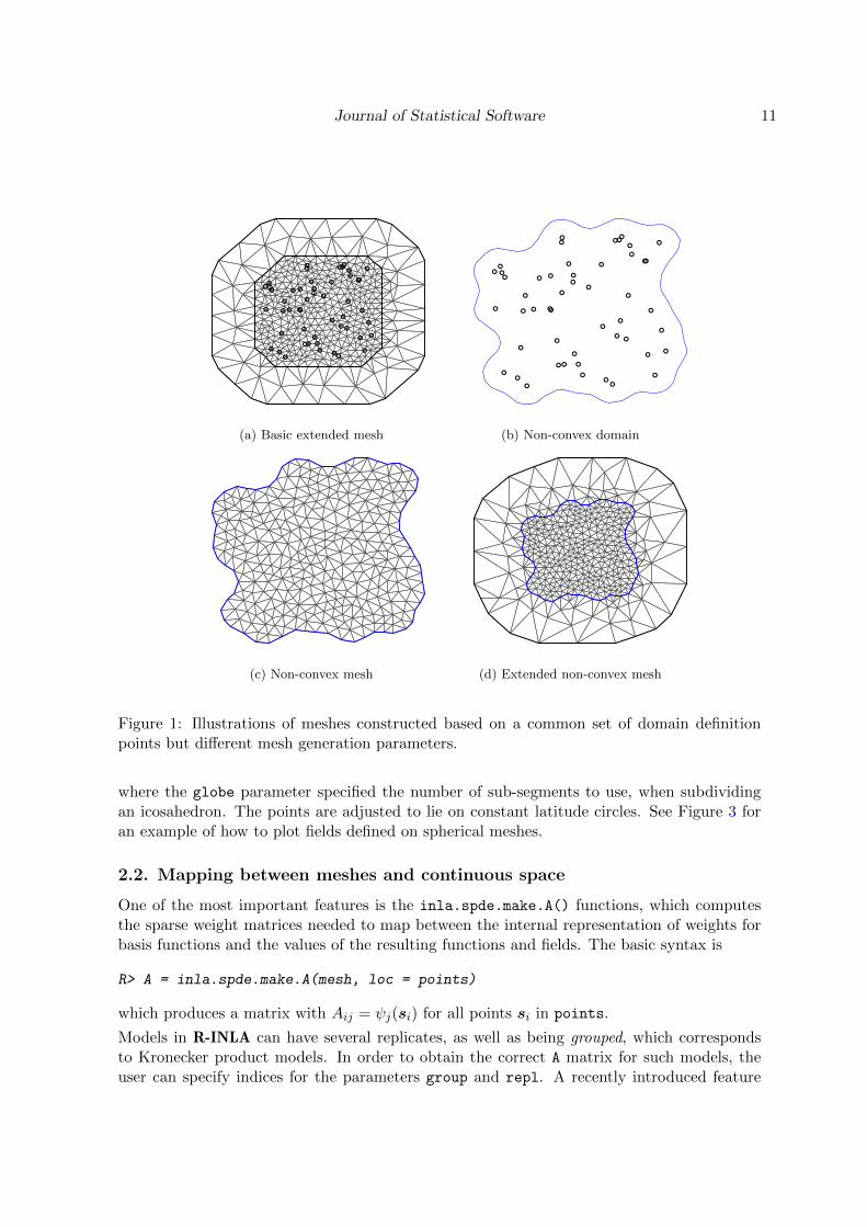
The aim is to create the triangulated mesh on top of which the SPDE/GMRF representationis to be built. The example in Figure 1 illustrates a common usage case, which is to have semi-randomly scattered observation locations in a region of space such that there is no physicalboundary, just a limited observation region. When dealing with only covariances betweendata points, this distinction is often unimportant, but here it becomes a possibly vital partof the model, since the SPDE will exhibit boundary effects. In the R-INLA implementation,Neumann boundaries are used, which increases the variance near the boundary. If we intendto model a stationary field across the entire domain of observations, we must therefore extendthe model domain far enough so that the boundary effects don’t influence the observations.However, note that the reverse is also true: if there is a physical boundary, the boundary

http://www.r-inla.org

http://code.google.com/p/inla/


effects may actually be desirable. The function inla.mesh.2d() allows us to create a meshwith small triangles in the domain of interest, and use larger triangles in the extension usedto avoid boundary effects. This minimises the extra computational work needed due to theextension.

R> m = 50

R> points = matrix(runif(m * 2), m, 2)

R> mesh = inla.mesh.2d(

+ loc = points, cutoff = 0.05, offset = c(0.1, 0.4), max.edge = c(0.05, 0.5) )

The cutoff parameter is used to avoid building many small triangles around clustered inputlocations, offset specifies the size of the inner and outer extensions around the data locations,and max.edge specifies the maximum allowed triangle edge lengths in the inner domain andin the outer extension. The overall effect of the triangulation construction is that, if desired,one can have smaller triangles, and hence higher accuracy of the field representation, wherethe observation locations are dense, larger triangles where data is more sparse (and henceprovides less detailed information), and large triangles where there is no data and spendingcomputational resources would be wasteful. However, note that there is neither any guaranteenor any requirement that the observation locations are included as nodes in the mesh. If oneso desires, the mesh can be designed from different principles, such as lattice points with norelation to the precise measurement locations. This emphasises the decoupling between thecontinuous domain of the field model and the discrete data locations.

A new feature is the option to compute a non-convex covering to use as boundary information,

R> bnd = inla.nonconvex.hull(points, convex = 0.12)

with the resulting domain boundary shown in Figure 1b. The boundary is then supplied toinla.mesh.2d(),

R> mesh = inla.mesh.2d(boundary = bnd, cutoff = 0.05, max.edge = c(0.1) )

resulting in the non-convex mesh shown in Figure 1c. Just as before, the SPDE edge effectscan be moved outside the domain of interest using an extension with larger triangles, shownin Figure 1d:

R> mesh = inla.mesh.2d(

+ boundary = bnd, cutoff = 0.05, offset = c(1, 0.5), max.edge = c(0.1, 0.5) )

For geostatistical problems with global data, one can work directly on a spherical mesh. Anyspatial coordinates must first be converted into 3D Cartesian coordinates. For longitudesand latitudes this can be done with inla.mesh.map(), and the result can be used withinla.mesh.2d():

R> loc.cartesian = inla.mesh.map(loc.longlat, projection = "longlat")

R> mesh2 = inla.mesh.2d(loc = loc.cartesian, ...)

Alternatively, a semi-regular mesh can be constructed using the more low-level command

R> mesh2 = inla.mesh.create(globe = 10)


(a) Basic extended mesh

(b) Non-convex domain

(c) Non-convex mesh (d) Extended non-convex mesh

Figure 1: Illustrations of meshes constructed based on a common set of domain definitionpoints but different mesh generation parameters.

where the globe parameter specified the number of sub-segments to use, when subdividingan icosahedron. The points are adjusted to lie on constant latitude circles. See Figure 3 foran example of how to plot fields defined on spherical meshes.

2.2. Mapping between meshes and continuous space

One of the most important features is the inla.spde.make.A() functions, which computesthe sparse weight matrices needed to map between the internal representation of weights forbasis functions and the values of the resulting functions and fields. The basic syntax is

R> A = inla.spde.make.A(mesh, loc = points)

which produces a matrix with Aij = ψj(si) for all points si in points.

Models in R-INLA can have several replicates, as well as being grouped, which correspondsto Kronecker product models. In order to obtain the correct A matrix for such models, theuser can specify indices for the parameters group and repl. A recently introduced feature


also allows specifying a one dimensional group.mesh, which is then interpreted as defining aKronecker product basis, such as for the space-time models mentioned in Section 1.1, and anexample is given in Section 3.2.

2.3. SPDE model construction

As the theory and practice evolves, new internal SPDE representation models are imple-mented. The current development focuses on models with internal name spde2. To find outwhat the currently available user-accessible models are, use the function inla.spde.models().

Defining an SPDE model object can now be as simple as

R> spde = inla.spde2.matern(mesh, alpha = 2)

but in practice we need to also specify the prior distribution for the parameters, and/or modifythe parameterisation to suit the specific situation. This is true in particular when the modelsare used as simple smoothers, as there is then rarely enough information in the likelihood tofully identify the parameters, giving more importance to the prior distributions.

Using the theory from Section 1.1, the empirically derived range expression ρ =√

8ν/κ allowsfor construction of a model with known range and variance (= 1) for (θ1, θ2) = (0, 0), via

R> sigma0 = 1

R> size = min(c(diff(range(mesh$loc[, 1])), diff(range(mesh$loc[, 2]))))

R> range0 = size / 5

R> kappa0 = sqrt(8) / range0

R> tau0 = 1 / (sqrt(4 * pi) * kappa0 * sigma0)

R> spde = inla.spde2.matern(mesh,

+ B.tau = cbind(log(tau0), -1, +1),

+ B.kappa = cbind(log(kappa0), 0, -1),

+ theta.prior.mean = c(0, 0),

+ theta.prior.prec = c(0.1, 1) )

Here, sigma0 is the field standard deviation and range0 is the spatial range for θ = 0,and B.tau and B.kappa are matrices storing the parameter basis functions introduced inSection 1.1. For stationary models, only the first matrix row needs to be supplied. In thisexample, the prior median for the spatial range is chosen heuristically to be a fifth of theapproximate domain diameter.

Setting suitable priors for θ in these models generally is difficult problem. The heuristicused above is to specify a fairly vague prior for θ1 which controls the variance, with σ2

0 beingthe median prior variance, and a larger prior precision for θ2. When range0 is a fifth ofthe domain size, the precision 1 for θ2 gives an approximate 95% prior probability for therange being shorter than the domain size. Experimental helper functions for constructingparameterisations and priors are included in the package.

Models with range larger than the domain size are usually indistinguishable from intrinsicrandom fields, which can be modelled by fixing κ to zero (or rather some small positivevalue) with B.tau = cbind(log(tau0), 1) and B.kappa = cbind(log(small), 0). Notethat the sum-to-zero constraints often used for lattice based intrinsic Markov models is in-appropriate due to the irregular mesh structure, and a weighted sum-to-zero constraint is


0.2

0.4

0.6

0.8

0.2 0.4 0.6 0.8

−10

−8

−6

−4

−2

0

2

4

6

8

0.2

0.4

0.6

0.8

0.2 0.4 0.6 0.8

−10

−8

−6

−4

−2

0

2

4

6

8

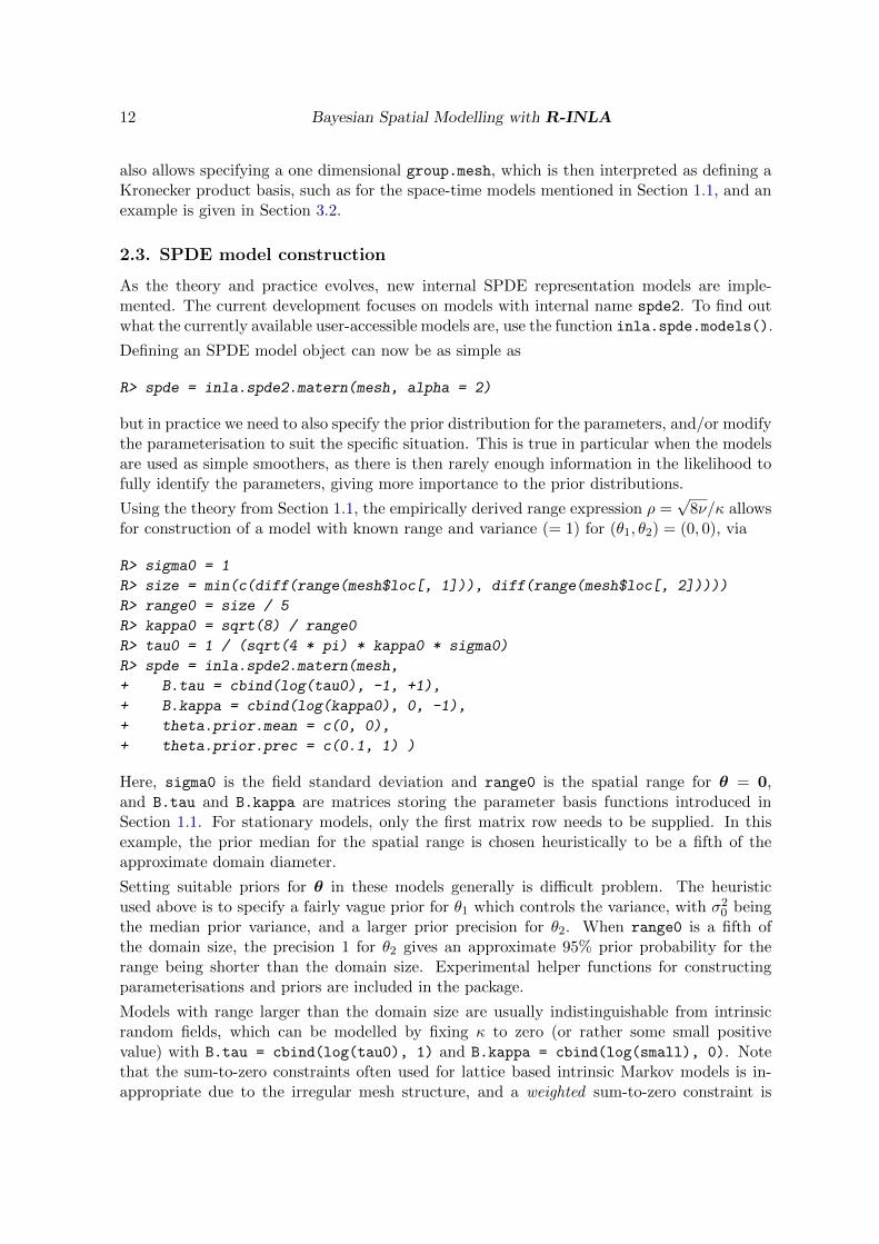
Figure 2: The two random field samples, with only the domain of interest, [0, 1]×[0, 1], shown.

needed to reproduce such models. The option constr = TRUE to the inla.spde.matern()

call can be used to apply an integrate-to-zero constraint instead, which uses the triangle ge-ometry to calculate the needed weights. Further integration constraints can be specified usingextraconstr.int = list(A = A, e = e) option, which implements constraints of the form

ACx = e,

where C is the sparse matrix with elements Cij =∫

Ω ψi(s)ψj(s) ds. Non-integration con-straints can be supplied with extraconstr, and all constraints will be passed on automaticallyto the inla() call later.

Properties and sampling

There are several helper functions for querying properties about spde model objects, the mostimportant one being inla.spde.precision(). To obtain the precision for the constructedmodel, with standard deviation a factor 3 larger than the prior median value, and range equalto the prior median, use

R> Q = inla.spde.precision(spde, theta=c(log(3), 0))

The following code then generates two samples from the model,

R> x = inla.qsample(n = 2, Q)

and the resulting fields are shown in Figure 2. To take any constraints specified in the spde

object into account when sampling, use

R> x = inla.qsample(n = 2, Q, constr = spde$f$extraconstr)


Obtaining covariances is a much more costly operation, but the function inla.qinv(Q) canquickly calculate all covariances between neighbours (in the Markov sense), including themarginal variances. Finally, inla.qsolve(Q,b) uses the internal R-INLA methods for solvinga linear system involving Q.

2.4. Plotting

Mesh structure

The interface supports a plot() function aimed at plotting the basic structure of a triangu-lation mesh. By specifying rgl = TRUE, the rgl plotting system is used, which is useful inparticular for spherical domains. Variations of the following commands were used to produceFigure 1:

R> plot(mesh)

R> plot(mesh, rgl = TRUE)

R> lines(mesh$segm$bnd, mesh$loc, add = FALSE)

Spatial fields

For plotting fields defined on meshes, one option is to use the rgl option, which supportsspecifying colour values for the nodes, producing an interpolated field plot, and optionallydraw triangle edges and vertices in the same plot:

R> plot(mesh, rgl = TRUE, col = x[, 1],

+ color.palette = function(n) grey.colors(n, 1, 0),

+ draw.edges = FALSE, draw.segments = TRUE, draw.vertices = FALSE)

The more common option is to explicitly evaluate the field on a regular lattice, and use anymatrix-based plotting mechanism, such as image():

R> proj = inla.mesh.projector(mesh, dims = c(100, 100))

R> image(proj$x, proj$y, inla.mesh.project(proj, field = x[, 1]))

All the figures showing fields have been drawn using a wrapper around the levelplot() fromthe lattice package, which is available in the supplementary material.

The inla.mesh.project/or() functions are here used to map between the basis functionweights for the mesh nodes and points on a regular grid, by default a 100 × 100 latticecovering the mesh domain. The functions also support several types of projections for sphericaldomains,

R> mesh2 = inla.mesh.create(globe = 10)

R> proj2a = inla.mesh.projector(mesh2, projection = "longlat", dims = c(361, 181))

R> proj2b = inla.mesh.projector(mesh2, projection = "mollweide", dims = c(361, 181))

with projected fields shown in Figure 3.


Lon−Lat projection

Longitude

Latit

ude

−50

0

50

−100 0 100

−3.4

−3.2

−3.0

−2.8

−2.6

Mollweide projection

−0.5

0.0

0.5

−1 0 1

−3.4

−3.2

−3.0

−2.8

−2.6

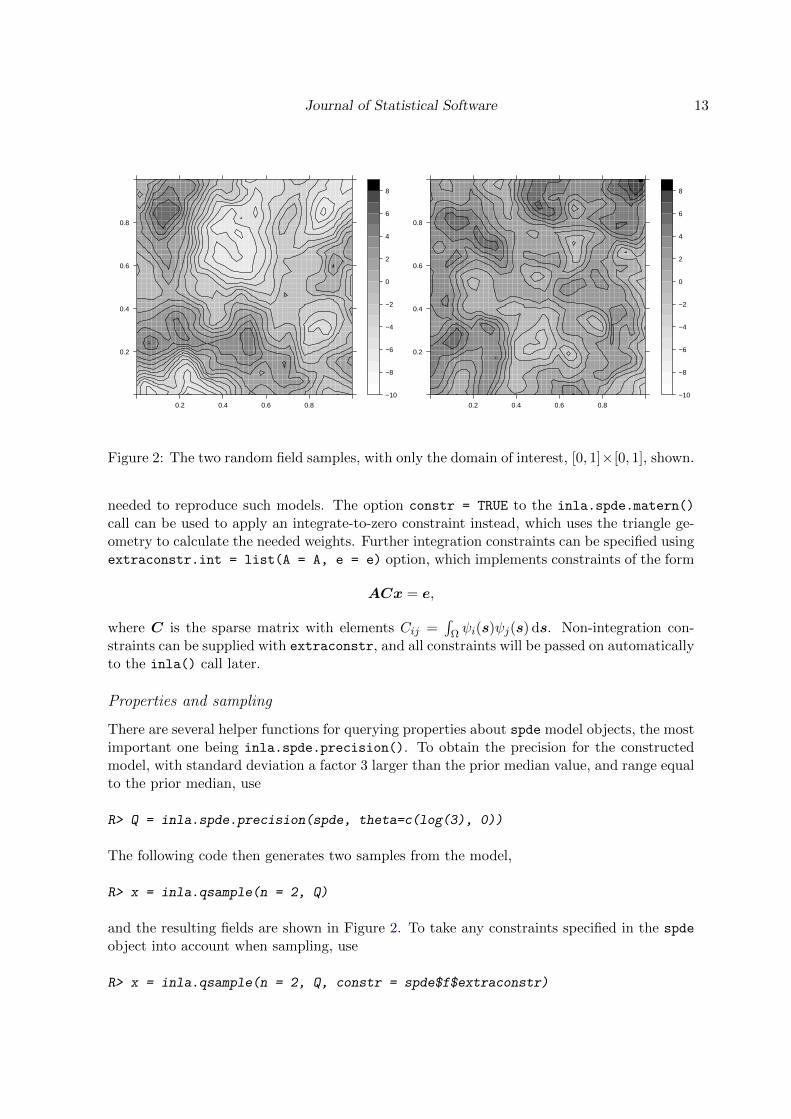
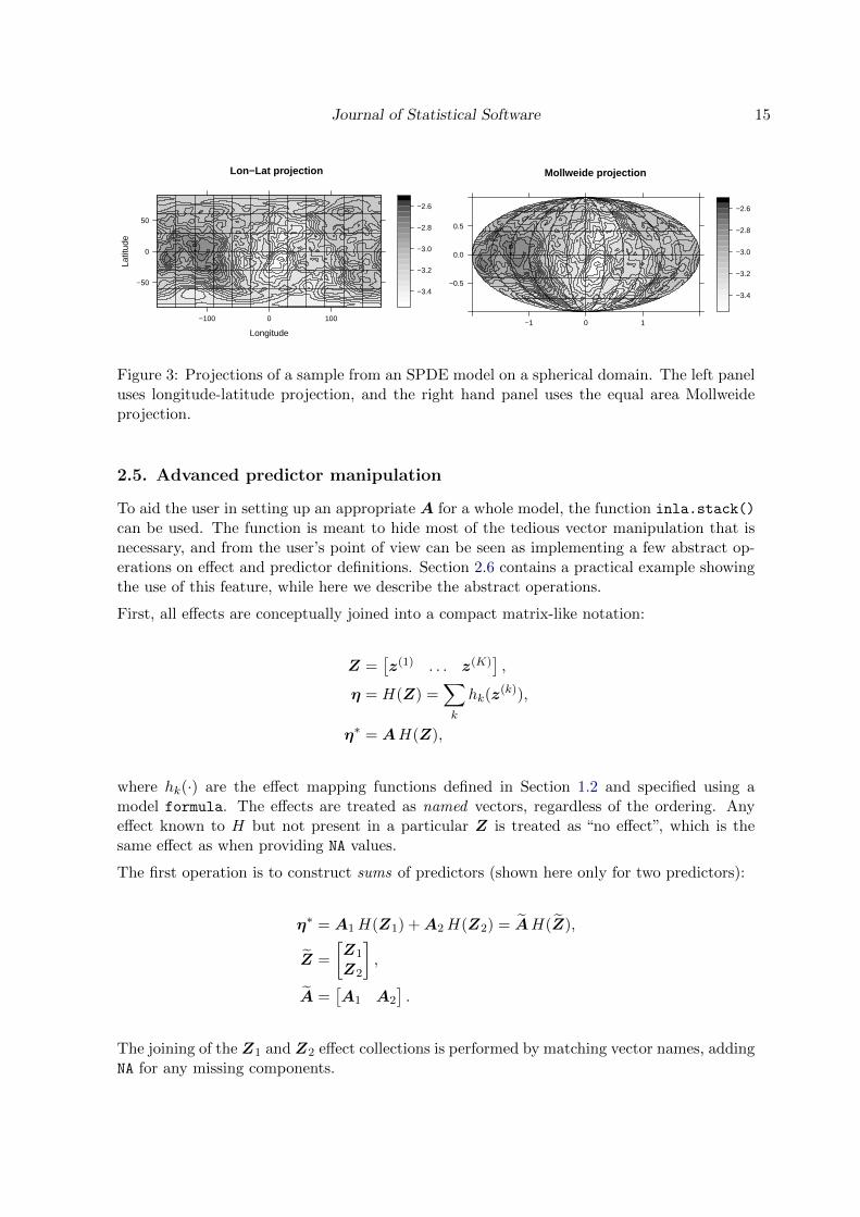
Figure 3: Projections of a sample from an SPDE model on a spherical domain. The left paneluses longitude-latitude projection, and the right hand panel uses the equal area Mollweideprojection.

2.5. Advanced predictor manipulation

To aid the user in setting up an appropriate A for a whole model, the function inla.stack()

can be used. The function is meant to hide most of the tedious vector manipulation that isnecessary, and from the user’s point of view can be seen as implementing a few abstract op-erations on effect and predictor definitions. Section 2.6 contains a practical example showingthe use of this feature, while here we describe the abstract operations.

First, all effects are conceptually joined into a compact matrix-like notation:

Z =[z(1) . . . z(K)

],

η = H(Z) =∑k

hk(z(k)),

η∗ = AH(Z),

where hk(·) are the effect mapping functions defined in Section 1.2 and specified using amodel formula. The effects are treated as named vectors, regardless of the ordering. Anyeffect known to H but not present in a particular Z is treated as “no effect”, which is thesame effect as when providing NA values.

The first operation is to construct sums of predictors (shown here only for two predictors):

η∗ = A1H(Z1) +A2H(Z2) = AH(Z),

Z =

[Z1

Z2

],

A =[A1 A2

].

The joining of the Z1 and Z2 effect collections is performed by matching vector names, addingNA for any missing components.


The second operation is to join predictors in sequence (only two predictors shown):

η∗1 = A1H(Z1),

η∗2 = A2H(Z2),

η∗ = (η∗1, η∗2) = AH(Z),

Z =

[Z1

Z2

],

A =

[A1 00 A2

].

As a post-processing step for both operations, the new covariate matrix Z and matrix A areanalysed to detect any duplicate rows in Z or any all-zero columns in A, and those are bydefault removed in order to minimise the internal size of the model representation.

The syntax for a sum operation is

R> stack = inla.stack(data = list(...),

+ A = list(A1, A2, ...),

+ effects = list(list(...),

+ list(...),

+ ...),

+ tag = ...)

where each A matrix has an associated list of effects. A join operation is performed bysupplying two or more previously generated stack objects,

R> stack = inla.stack(stack1, stack2, ...)

Any vectors specified in the data list, most importantly the response variable vector itself,should be the same length as the predictor itself (scalars are replicated to the appropriatelength). With the help of the name-tag it also keeps track of the indices needed to map fromthe original inputs into the resulting stacked representation. See Section 2.6 for an illustratingexample of using inla.stack().

Note that H(·) is conceptually defined by the model formula, which needs to mention everycovariate component present in Z and that is meant to be used.

2.6. Bayesian inference

In this section we will look at a simple example of how to use the SPDE models in latentGaussian models when doing direct Bayesian inference based on the INLA method describedin Section 1.2.

Consider a simple Gaussian linear model involving two independent realisations (replicates) ofa latent spatial field x(s), observed at the same m locations, s1, . . . , sm, for each replicate.For each i = 1, . . . ,m,

yi = β0 + ciβc + x1(si) + ei,

yi+m = β0 + ci+mβc + x2(si) + ei+m,


where ci is an observation-specific covariate, ei is measurement noise, and x1(·) and x2(·) arethe two field replicates. Note that the intercept, β0, can be interpreted as a spatial covariateeffect, constant over the domain.

We use the basis function representation of x(·) to define a sparse matrix of weights A suchthat x(si) =

∑j Aijxj , where xj is the joint set of weights for the two replicate fields.

If we only had one replicate, we would have Aij = ψj(si). The matrix can be generatedby inla.spde.make.A(), which locates the points in the mesh and organises the evaluatedvalues of the basis functions for the two replicates:

R> A = inla.spde.make.A(mesh,

+ loc = points,

+ index = rep(1:m, times = 2),

+ repl = rep(1:2, each = m) )

For each observation, index gives the corresponding index into the matrix of measurementlocations, and repl determines the corresponding replicate index. In case of missing observa-tions, one can either keep this A-matrix while setting the corresponding elements of the datavector y to NA, or omit the corresponding elements from y as well as from the index and repl

parameters above. Also note that the row-sums of A are 1, since the piece-wise linear basisfunctions we use sum to 1 at each location.

Rewriting the observation model in vector form gives

y = 1β0 + cβc +Ax+ e

= A(x+ 1β0) + cβc + e

Using the helper functions, we can generate data using our two previously simulated modelreplicates,

R> x = as.vector(x)

R> covariate = rnorm(m * 2)

R> y = 5 + covariate * 2 + as.vector(A %*% x) + rnorm(m * 2) * 0.1

The formula in inla() defines a linear predictor η as the sum of all effects, and an NA in acovariate or index vector is interpreted as no effect. To accommodate predictors that involvemore than one element of a random effect, one can specify a sparse matrix of weights definingan arbitrary linear combination of the elements of η, giving a new predictor vector η∗. Thelinear predictor output from inla() then contains the joint vector (η∗,η). To implement ourmodel, we separate the spatial effects from the covariate by defining

ηe =

[x+ 1β0

cβc

],

and construct the predictor as

η∗e = A(x+ 1β0) + cβc

=[A I

]ηe = Aeηe


so that now E(y | ηe) = η∗e. The bookkeeping required to describe this to inla() involvesconcatenating matrices and adding NA elements to the covariates and index vectors:

Ae =[A I2m

]field0 = (1, . . . , n, 1, . . . , n)

field = (field0, NA, . . . , NA)

intercept = (1, . . . , 1, NA, . . . , NA)

cov = (NA, . . . , NA, c1, . . . , c2m)

Doing this by hand with Matrix::cBind(), c(), and rep() quickly becomes tedious anderror-prone, so one can instead use the helper function inla.stack(), which takes blocks ofdata, weight matrices, and effects and joins them, adding NA where needed. Identity matricesand constant covariates can be abbreviated to scalars, with a complaint being issued if theinput is inconsistent or ambiguous.

We also need to keep track of the two field replicates, and use inla.spde.make.index(),which gives a list of index vectors for indexing the full mesh and its replicates (it can also beused for indexing Kronecker product group models, e.g., in simple multivariate and spatio-temporal models). The code

R> mesh.index = inla.spde.make.index(name = "field",

+ n.spde = spde$n.spde,

+ n.repl = 2)

generates a list mesh.index with three index vectors,

field = (1, . . . , n, 1, . . . , n),

field.repl = (1, . . . , 1, 2, . . . , 2),

field.group = (1, . . . , 1, 1, . . . , 1).

The predictor information for the observed data can now be collected, using

R> st.est = inla.stack(data = list(y = y),

+ A = list(A, 1),

+ effects = list(c(mesh.index, list(intercept = 1)),

+ list(cov = covariate)),

+ tag = "est")

where the tag identifier can later be used for identifying the correct indexing into the inla()

output. As discussed in Section 2.5, each“A”matrix must have an associated list of“effects”,in this case A:(field, field.repl, field.group, intercept) and 1:(cov). The data listmay contain anything associated with the “left hand side” of the model, such as exposure E

for Poisson likelihoods. By default, duplicates in the effects are identified and replaced bysingle copies (compress = TRUE), and effects that do not affect η∗ are removed completely(remove.unused = TRUE), so that each column of the resulting A matrix has a least onenon-zero element.


If we want to obtain the posterior prediction of the combined spatial effects at the meshnodes, x(si) + β0, we can define

ηp = x+ 1β0

η∗p = Iηp = Apηp

and construct the corresponding information stack with

R> st.pred = inla.stack(data = list(y = NA),

+ A = list(1),

+ effects = list(c(mesh.index, list(intercept = 1))),

+ tag = "pred")

We can now join the estimation and prediction stack into a single stack,

R> stack = inla.stack(st.est, st.pred)

and the result is simplified by removing duplicated effects:

η∗s =

[Ae 00 Ap

] [ηeηp

]=

[A I 00 0 I

]x+ 1β0

cβcx+ 1β0

=

[A II 0

] [x+ 1β0

cβc

]= Asηs

In this simple example, the second block row of As (generating x+1β0) is not strictly needed,since the same information would be available in ηs itself if we specified remove.unused =

FALSE when constructing stack.pred and stack, but in general such special cases can behard to keep track of.

We are now ready to do the actual estimation. Note that we must explicitly remove the defaultintercept from the η-model, since that would otherwise be applied twice in the constructionof η∗, and the constant covariate intercept is used instead:

R> formula =

+ y ~ -1 + intercept + cov + f(field, model = spde, replicate = field.repl)

R> inla.result = inla(formula,

+ data = inla.stack.data(stack, spde = spde),

+ family = "normal",

+ control.predictor = list(A = inla.stack.A(stack),

+ compute = TRUE))

The function inla.stack.data() produces the list of variables needed to evaluate the formulaand inla.stack.A() extracts the As matrix.

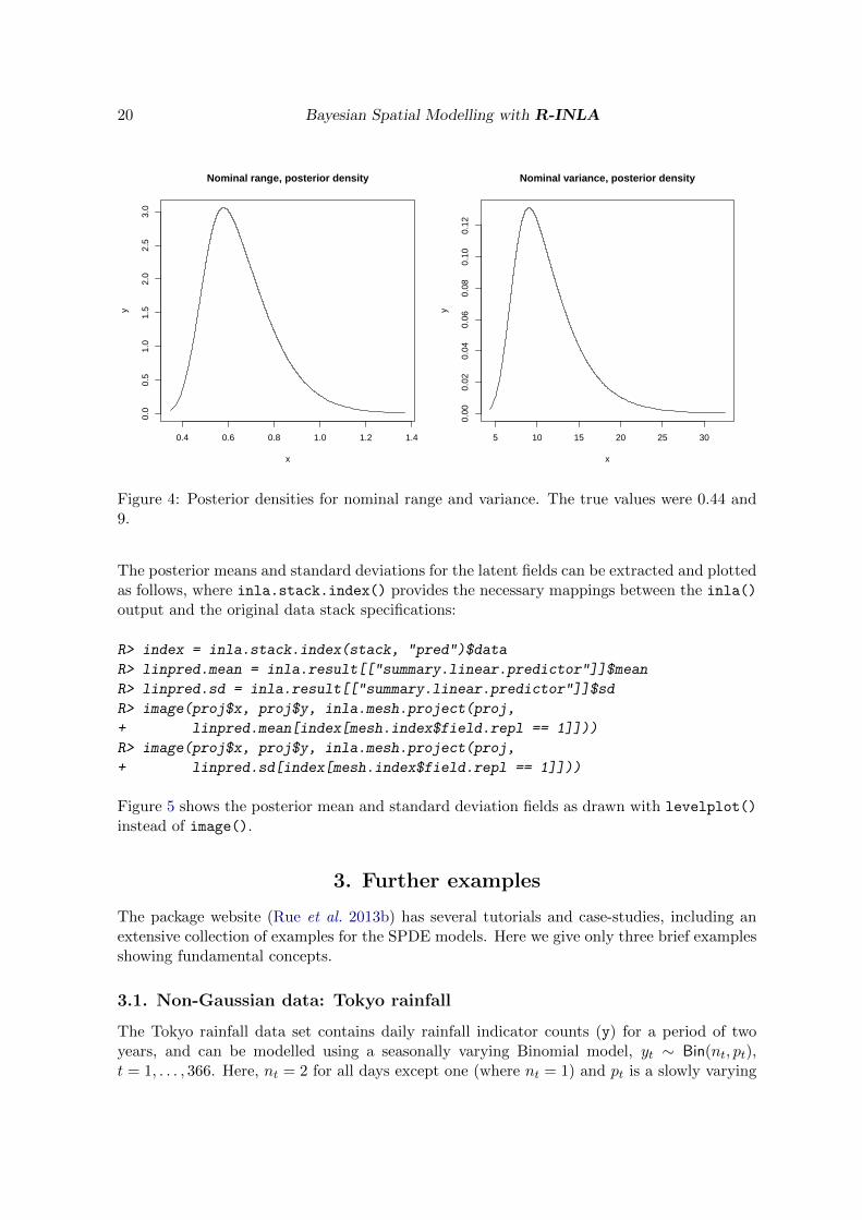
Since the SPDE-related contents of inla.result can be hard to interpret, the helper functioninla.spde2.result() can be used to extract the relevant parts and transform them into moreuser-friendly information, such as posterior densities for range and variance instead of rawdistributions for θ, as shown in Figure 4:

R> result = inla.spde2.result(inla.result, "field", spde)

R> plot(result[["marginals.range.nominal"]][[1]], type = "l",

+ main = "Nominal range, posterior density")


0.4 0.6 0.8 1.0 1.2 1.4

0.0

0.5

1.0

1.5

2.0

2.5

3.0

Nominal range, posterior density

x

y

5 10 15 20 25 30

0.00

0.02

0.04

0.06

0.08

0.10

0.12

Nominal variance, posterior density

x

y

Figure 4: Posterior densities for nominal range and variance. The true values were 0.44 and9.

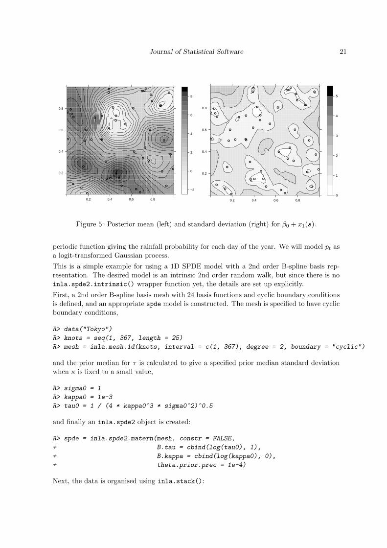
The posterior means and standard deviations for the latent fields can be extracted and plottedas follows, where inla.stack.index() provides the necessary mappings between the inla()

output and the original data stack specifications:

R> index = inla.stack.index(stack, "pred")$data

R> linpred.mean = inla.result[["summary.linear.predictor"]]$mean

R> linpred.sd = inla.result[["summary.linear.predictor"]]$sd

R> image(proj$x, proj$y, inla.mesh.project(proj,

+ linpred.mean[index[mesh.index$field.repl == 1]]))

R> image(proj$x, proj$y, inla.mesh.project(proj,

+ linpred.sd[index[mesh.index$field.repl == 1]]))

Figure 5 shows the posterior mean and standard deviation fields as drawn with levelplot()

instead of image().

3. Further examples

The package website (Rue et al. 2013b) has several tutorials and case-studies, including anextensive collection of examples for the SPDE models. Here we give only three brief examplesshowing fundamental concepts.

3.1. Non-Gaussian data: Tokyo rainfall

The Tokyo rainfall data set contains daily rainfall indicator counts (y) for a period of twoyears, and can be modelled using a seasonally varying Binomial model, yt ∼ Bin(nt, pt),t = 1, . . . , 366. Here, nt = 2 for all days except one (where nt = 1) and pt is a slowly varying


0.2

0.4

0.6

0.8

0.2 0.4 0.6 0.8

−2

0

2

4

6

8

0.2

0.4

0.6

0.8

0.2 0.4 0.6 0.8

0

1

2

3

4

5

Figure 5: Posterior mean (left) and standard deviation (right) for β0 + x1(s).

periodic function giving the rainfall probability for each day of the year. We will model pt asa logit-transformed Gaussian process.

This is a simple example for using a 1D SPDE model with a 2nd order B-spline basis rep-resentation. The desired model is an intrinsic 2nd order random walk, but since there is noinla.spde2.intrinsic() wrapper function yet, the details are set up explicitly.

First, a 2nd order B-spline basis mesh with 24 basis functions and cyclic boundary conditionsis defined, and an appropriate spde model is constructed. The mesh is specified to have cyclicboundary conditions,

R> data("Tokyo")

R> knots = seq(1, 367, length = 25)

R> mesh = inla.mesh.1d(knots, interval = c(1, 367), degree = 2, boundary = "cyclic")

and the prior median for τ is calculated to give a specified prior median standard deviationwhen κ is fixed to a small value,

R> sigma0 = 1

R> kappa0 = 1e-3

R> tau0 = 1 / (4 * kappa0^3 * sigma0^2)^0.5

and finally an inla.spde2 object is created:

R> spde = inla.spde2.matern(mesh, constr = FALSE,

+ B.tau = cbind(log(tau0), 1),

+ B.kappa = cbind(log(kappa0), 0),

+ theta.prior.prec = 1e-4)

Next, the data is organised using inla.stack():


R> A = inla.spde.make.A(mesh, loc = Tokyo$time)

R> time.index = inla.spde.make.index("time", n.spde = spde$n.spde)

R> stack = inla.stack(data = list(y = Tokyo$y, link = 1, Ntrials = Tokyo$n),

+ A = list(A),

+ effects = list(time.index),

+ tag = "est")

R> formula = y ~ -1 + f(time, model = spde)

R> data = inla.stack.data(stack)

R> result = inla(formula, family = "binomial", data = data,

+ Ntrials = data$Ntrials,


+ link = data$link,

+ compute = TRUE))

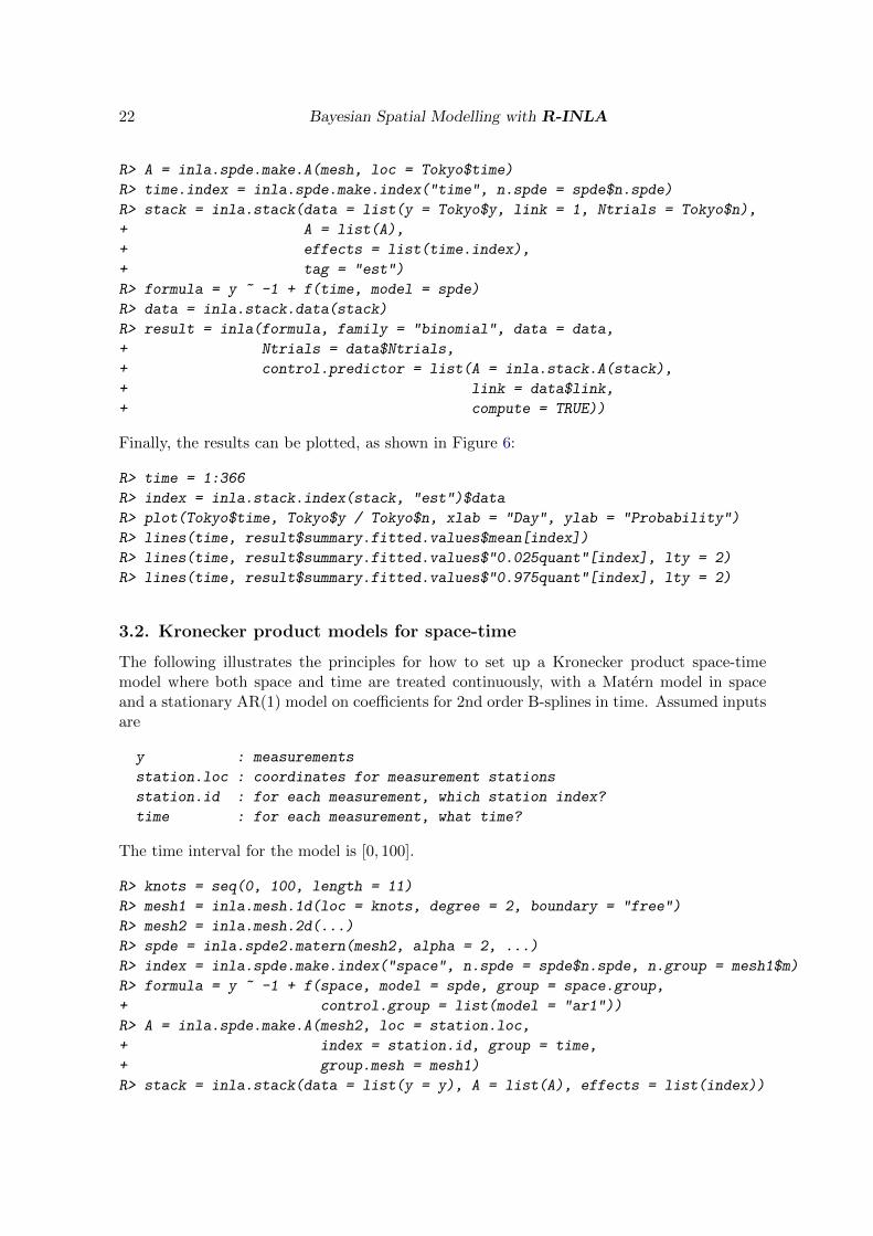
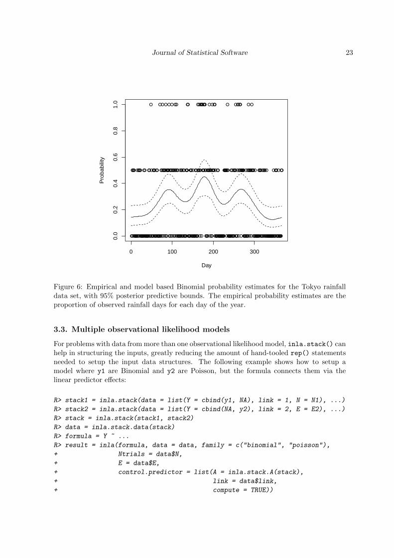
Finally, the results can be plotted, as shown in Figure 6:

R> time = 1:366

R> index = inla.stack.index(stack, "est")$data

R> plot(Tokyo$time, Tokyo$y / Tokyo$n, xlab = "Day", ylab = "Probability")

R> lines(time, result$summary.fitted.values$mean[index])

R> lines(time, result$summary.fitted.values$"0.025quant"[index], lty = 2)

R> lines(time, result$summary.fitted.values$"0.975quant"[index], lty = 2)

3.2. Kronecker product models for space-time

The following illustrates the principles for how to set up a Kronecker product space-timemodel where both space and time are treated continuously, with a Matern model in spaceand a stationary AR(1) model on coefficients for 2nd order B-splines in time. Assumed inputsare

y : measurements

station.loc : coordinates for measurement stations

station.id : for each measurement, which station index?

time : for each measurement, what time?

The time interval for the model is [0, 100].

R> knots = seq(0, 100, length = 11)

R> mesh1 = inla.mesh.1d(loc = knots, degree = 2, boundary = "free")

R> mesh2 = inla.mesh.2d(...)

R> spde = inla.spde2.matern(mesh2, alpha = 2, ...)

R> index = inla.spde.make.index("space", n.spde = spde$n.spde, n.group = mesh1$m)

R> formula = y ~ -1 + f(space, model = spde, group = space.group,

+ control.group = list(model = "ar1"))

R> A = inla.spde.make.A(mesh2, loc = station.loc,

+ index = station.id, group = time,

+ group.mesh = mesh1)

R> stack = inla.stack(data = list(y = y), A = list(A), effects = list(index))


0 100 200 300

0.0

0.2

0.4

0.6

0.8

1.0

Day

Pro

babi

lity

Figure 6: Empirical and model based Binomial probability estimates for the Tokyo rainfalldata set, with 95% posterior predictive bounds. The empirical probability estimates are theproportion of observed rainfall days for each day of the year.

3.3. Multiple observational likelihood models

For problems with data from more than one observational likelihood model, inla.stack() canhelp in structuring the inputs, greatly reducing the amount of hand-tooled rep() statementsneeded to setup the input data structures. The following example shows how to setup amodel where y1 are Binomial and y2 are Poisson, but the formula connects them via thelinear predictor effects:

R> stack1 = inla.stack(data = list(Y = cbind(y1, NA), link = 1, N = N1), ...)

R> stack2 = inla.stack(data = list(Y = cbind(NA, y2), link = 2, E = E2), ...)

R> stack = inla.stack(stack1, stack2)

R> data = inla.stack.data(stack)

R> formula = Y ~ ...

R> result = inla(formula, data = data, family = c("binomial", "poisson"),

+ Ntrials = data$N,

+ E = data$E,


+ link = data$link,

+ compute = TRUE))


4. Future development

The R-INLA package is in constant development, with new models added as they are neededand developed. The current work for the SPDE models is focusing on construction of param-eter basis functions and priors for non-stationary model parameters, as well as implementingextensions to non-separable space-time models and more flexible boundary conditions. Anassociated package excursions for computing level excursion sets with joint excursion probabil-ities, as well as credible regions for contour curves, is available in CRAN (Bolin and Lindgren2014).

As the size of spatial and spatio-temporal models and data sets grows, iterative matrix meth-ods and other approximation techniques for more complex models are also being investigated,with the long-term goal of replacing the core of R-INLA to more easily handle such challenges.

Acknowledgements

The authors wish to thank their collaborators David Bolin, Michela Cameletti, Janine Illian,Johan Lindstrom, Thiago Martins, Daniel Simpson, Sigrunn Sørbye, Elias Krainski, andRyan Yue, who have all contributed with ideas and suggestions for the development of thespatial model interface. We are also grateful to the editors and reviewers for their thoughtfulcomments on the manuscript.

References

Banerjee S, Gelfand AE, Finley AO, Sang H (2008). “Gaussian Predictive Process Models forLarge Spatial Datasets.” Journal of the Royal Statistical Society B, 70(4), 825–848.

Besag J (1981). “On a System of Two-dimensional Recurrence Equations.” Journal of theRoyal Statistical Society B, 43(3), 302–309.

Besag J, Mondal D (2005). “First-order Intrinsic Autoregressions and the de Wijs Process.”Biometrika, 92(4), 909–920.

Bolin D, Lindgren F (2011). “Spatial Models Generated by Nested Stochastic Partial Differ-ential Equations, with an Application to Global Ozone Mapping.” The Annals of AppliedStatistics, 5(1), 523–550. ISSN 1932-6157.

Bolin D, Lindgren F (2013). “A Comparison Between Markov Approximations and OtherMethods for Large Spatial Data Sets.” Computational Statistics and Data Analysis, 61,7–21.

Bolin D, Lindgren F (2014). “Excursion and contour uncertainty regions for latent Gaussianmodels.” Journal of the Royal Statistical Society B. ISSN 1467-9868. doi:10.1111/rssb.12055.

Cameletti M, Lindgren F, Simpson D, Rue H (2013). “Spatio-temporal Modeling of Partic-ulate Matter Concentration through the SPDE Approach.” AStA Advances in StatisticalAnalysis, 97(2), 109–131. ISSN 1863-8171. doi:10.1007/s10182-012-0196-3.

http://dx.doi.org/10.1111/rssb.12055


http://dx.doi.org/10.1007/s10182-012-0196-3


Cressie NAC, Johannesson G (2008). “Fixed Rank Kriging for Very Large Spatial Data Sets.”Journal of the Royal Statistical Society B, 70(1), 209–226.

Lindgren F, Rue H, Lindstrom J (2011). “An Explicit Link Between Gaussian Fields andGaussian Markov Random Fields: the Stochastic Partial Differential Equation Approach.”Journal of the Royal Statistical Society B, 73(4), 423–498. ISSN 1369-7412.

Lindgren G, Lindgren F (2011). “Stochastic Asymmetry Properties of 3D Gauss-LagrangeOcean Waves with Directional Spreading.” Stochastic Models, 27(3), 490–520. ISSN 1532-6349.

Martins TG, Simpson D, Lindgren F, Rue H (2013). “Bayesian Computing with INLA: NewFeatures.” Computational Statistics and Data Analysis, 67, 68–83.

Nychka D, Hammerling D, Sain S, Lenssen N (2013). LatticeKrig: Multiresolution Krig-ing based on Markov Random Fields. URL http://cran.r-project.org/web/packages/

LatticeKrig/.

Rozanov A (1982). Markov Random Fields. Springer-Verlag, New York.

Rue H, Martino S, Chopin N (2009). “Approximate Bayesian Inference for Latent GaussianModels using Integrated Nested Laplace Approximations (with discussion).” Journal of theRoyal Statistical Society B, 71, 319–392.

Rue H, Martino S, Lindgren F, Simpson D, Riebler A (2013a). Code Repository for R-INLA: Approximate Bayesian Inference using Integrated Nested Laplace Approximations.URL http://code.google.com/p/inla/.

Rue H, Martino S, Lindgren F, Simpson D, Riebler A (2013b). R-INLA: ApproximateBayesian Inference using Integrated Nested Laplace Approximations. Trondheim, Norway.URL http://www.r-inla.org/.

Sigrist F, Kunsch HR, Stahel WA (2014). “Stochastic partial differential equation basedmodelling of large space-time data sets.” Journal of the Royal Statistical Society B. ISSN1467-9868. doi:10.1111/rssb.12061.

Simpson D, Lindgren F, Rue H (2012a). “In Order to Make Spatial Statistics ComputationallyFeasible, We Need to Forget About the Covariance Function.” Environmetrics, 23(1), 65–74. ISSN 1180-4009.

Simpson D, Lindgren F, Rue H (2012b). “Think Continuous: Markovian Gaussian Models inSpatial Statistics.” Spatial Statistics, 1, 16–29. ISSN 2211-6753.

Whittle P (1954). “On Stationary Processes in the Plane.” Biometrika, 41(3/4), 434–449.

Whittle P (1963). “Stochastic Processes in Several Dimensions.” Bull. Inst. Internat. Statist.,40, 974–994.

Wikle CK (2010). “Low-rank Representations for Spatial Processes.” In A Gelfand, P Diggle,M Fuentes, P Guttorp (eds.), Handbook of Spatial Statistics, pp. 107–118. Chapman andHall/CRC, Boca Raton, FL.

http://cran.r-project.org/web/packages/LatticeKrig/

http://cran.r-project.org/web/packages/LatticeKrig/

http://code.google.com/p/inla/

http://www.r-inla.org/



Affiliation:

Finn LindgrenDepartment of Mathematical SciencesUniversity of BathClaverton DownBA2 7AY, Bath, United KingdomE-mail: [email protected]: http://people.bath.ac.uk/fl353/

Journal of Statistical Software http://www.jstatsoft.org/

published by the American Statistical Association http://www.amstat.org/

Volume VV, Issue II Submitted: yyyy-mm-ddMMMMMM YYYY Accepted: yyyy-mm-dd

mailto:[email protected]

http://people.bath.ac.uk/fl353/

http://www.jstatsoft.org/

http://www.amstat.org/

Documents

Bayesian Spatial Modelling with R-INLAinla.r-inla-download.org/r-inla.org/papers/jss/lindgren.pdf · 2 Bayesian Spatial Modelling with R-INLA is that classical Gaussian random elds