Information retrieval by explicit inversion - Earth Online¥act as common platform for intercomparison ¥document discrepancies between or uncertainties ... (1902): ¤ For each set

Information retrieval by explicit inversion

Michel M. Verstraete

Frascati, 1 August 2006

1. How good are BRF models?

2. Principles of model inversion in a remote sensing

context

3. Look-Up Tables (LUT) approach

4. Applications

5. Exploiting RPV

Outline

Radiative Transfer Model Intercomparison

• Phase 1: March to August 1999

• Reference: Pinty et al. (2001)'Radiation Transfer ModelIntercomparison (RAMI)Exercise', Journal of GeophysicalResearch, 106, 11,937-11,956.

• Phase 2: February to June 2002

• Reference: Pinty et al. (2004)'RAdiation transfer ModelIntercomparison (RAMI) exercise:Results from the second phase',Journal of Geophysical Research,109, D0621010.1029/2003JD004252.

• Phase 3: Mars to December 2005(paper submitted)

• Home, protocols and results:http://rami-benchmark.jrc.it/

• Radiation Transfer (RT) models constitute an essential component

for the quantitative interpretation of remote sensing data

• The accuracy and reliability of the solutions to the inverse problems

are determined by the performance of both the RT models and the

remote sensing instruments

• The increase in data accuracy and BRF sampling of current RS

instruments will be better exploited if the uncertainties of the RT

models are decreased

• The establishment of a consensus on standards among the surface

BRF community should form the basis for its credibility with respect

to other scientific communities as well as decision and policy makers

Motivations for RT model evaluation

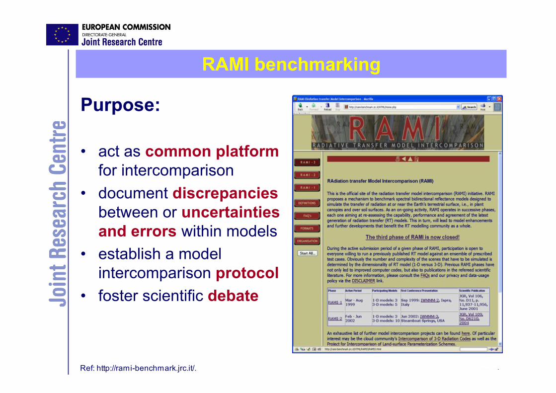
Purpose:

• act as common platform

for intercomparison

• document discrepancies

between or uncertainties

and errors within models

• establish a model

intercomparison protocol

• foster scientific debate

Ref: http://rami-benchmark.jrc.it/.

RAMI benchmarking

• RAMI-1 (1999):§ Turbid medium and discrete

§ Solar domain + purist corner

• RAMI-2 (2002):§ Topography + true “zoom-in”

• RAMI-3 (2005):§ Birch and conifer scene

(GO models)

§ Heterogeneous purist corner

§ Local transmission andhorizontal flux measurements

HOMogeneous HETerogeneous

RAMI-1 RAMI-2 RAMI-3

13

20

42

Fra

cti

on

of

HET

[%

]

Nu

mb

er

Ex

pe

rim

en

ts


660715

980

RAMI evolution

Tartu Observatory,EstoniaM. Möttus, A. KuuskFRT

CCRS, CanadaR. FernandesMAC

CCRS, CanadaN. Rochdie, R. Fernandes5scale

JRC, ItalyB. Pinty, T. Lavergne2stream

NLR, NetherlandsW. Verhoef4SAIL2

Cox, USAR. ThompsonSprint3

JRC, ItalyN. Gobron! discret

NLR, NetherlandsW. VerhoefSAIL++

JRC,ItalyT. Lavergneraytran

JRC, ItalyT. LavergneRayspread

Beijing N. Univ., ChinaD. Xie, W. QinRGM

NASA GFSC, USAW. Qinmbrf

NOVELTIS, FranceR. RuilobaHyemalis

UCL, UKP. Lewis, M. Disneyfrat

Univ. Swansea, UKP. NorthFLIGHT

UCL, UKM. Disney, P. Lewisdrat

CESBIO, FranceJ.P. Gastellu, E.MartinDART

Tartu Observatory,EstoniaA. KuuskACRM

AFFILIATIONPARTICIPANTMODEL NAME

3-D models

1-D models

new in RAMI-3


8

13

18

Num

ber

of

models


5

10

11/13

3

-D

models

Absorption

Albedo

Transmission

Measurements include

Flux quantities:

• Albedo

• Transmission

• Absorption

BRF quantities:

•Total BRF (PP+OP)

total BRF

multiple collided

single collided

single uncollided

BRF quantities:

•Total BRF (PP+OP)

•BRF components–multiple collided

–single uncollided(hit soil only once)

–single collided (hitleaves only once)

Measurement types

• In general, there is no absolute ‘truth’ available! Model results cannot be

evaluated against some reference standard.

• Laboratory data are difficult to use as reference standard due to incomplete

knowledge of the exact illumination, measurement, as well as (structural

and spectral) target properties.

but

• Model results can be compared against each other to document their

relative differences.

• Model results can be compared over ensembles of test scenarios

to establish trends/behaviours in their performance.

• Careful inspection/verification of an ensemble of model results may lead to

the establishment of the “most credible solutions” as a surrogate for the

“truth”.

RT model intercomparison caveats

( ) !"=

#=

models

;1models

0

200,,,

N

cmm

mcv

N$%&&'

( ) ( )( ) ( )!"##$!"##$

!"##$!"##$

,,,,,,

,,,,,,

ivmivc

ivmivc

+

%[ ]%

Model to ensemble differences:

Repeat for all available viewing, illumination, spectral, and structure

conditions.

Make histogram of values( )

mcv !"#$$% ,,,

0


Relative intercomparison (1)

( ) !"=

#=

models

;1models

0

200,,,

N

cmm

mcv

N$%&&'

( ) ( )( ) ( )!"##$!"##$

!"##$!"##$

,,,,,,

,,,,,,

ivmivc

ivmivc

+

%[ ]%

Model to ensemble differences:

Repeat for all available viewing, illumination, spectral, and structure

conditions.

Make histogram of values( )

mcv !"#$$% ,,,

0


RAMI-2 (5 models)

RAMI-3 (5 models)

RAMI-2 (8 models)

RAMI-3 (11 models)


Use !2 metric to identify how close RT models are to a credible

BRF solution:

( ) ( )[ ]( )!"

!#!#

;

;,,;,,2

2

i

jsijsi credible$( ) ! ! != = ="

=0

1 1 1

2

1

1# #

$%N

i

N

s

N

j

scenes v

N

( ) ( )!"!" ;,,;,,3D

jsijsicredible =

Credible BRF solution is derived from 3D Monte Carlo models:

Simulation error is fraction f of credible BRF solution:

( ) ( )!"!# ;,,,D3

jsifi =

Models with X2 " 1 are indiscernible from the !credible to withinf


Homogeneous

X2 uses "=0.03<BRF>3D

RAMI-2RAMI-3

DiscreteHeterogeneous

RAMI-2RAMI-3

Model performance improved from RAMI-2 to RAMI-3!




context


4. Applications

5. Exploiting RPV

Outline

Measurement interpretation

• A model representing a measurement expresses the dependency of thismeasurement with respect to the relevant variables:

),,,( 21 Msssfz L=

• where sm are the state variables of the system (here: target, environment,source of radiation, sensor)

• In principle, if the model is correct and if the values of all state variables smare known, such a model can accurately simulate the observation (directproblem)

• In practice, a quantity z* is measured, and one seeks information on thestate variables sm (inverse problem)

• If a single state variable accounts for the physics of the measurement, theproblem can be solved accurately (analytically or numerically):

• where s* is the estimate of the state variable retrieved from themeasurement z*, and ! stands for the error of measurement.

• In general, more than one state variable is required to describe the physicsof the problem. The solution of the inverse problem then requires multipleequations and therefore multiple measurements.

);()()( *1*** !! zfssfzsfz "=#+=#=

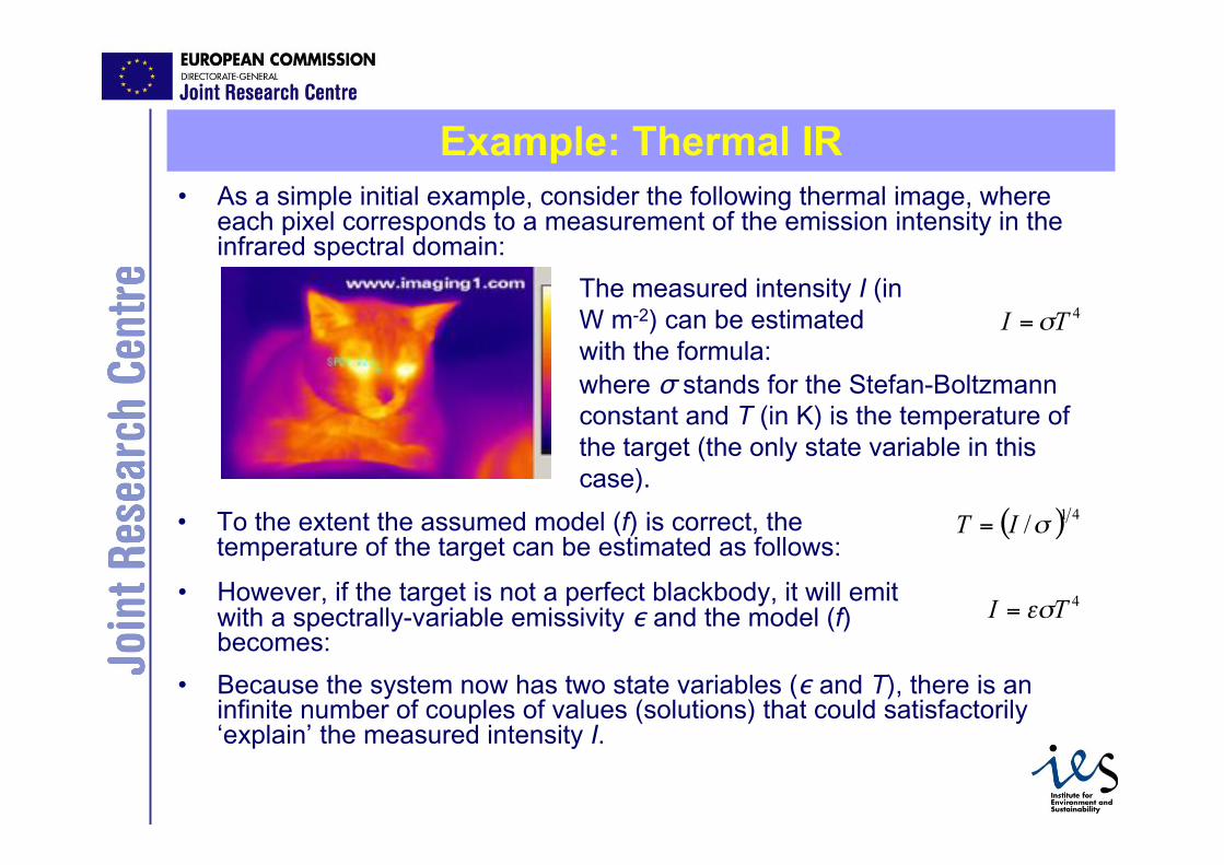
Example: Thermal IR

• As a simple initial example, consider the following thermal image, whereeach pixel corresponds to a measurement of the emission intensity in theinfrared spectral domain:

4TI !=

• To the extent the assumed model (f) is correct, thetemperature of the target can be estimated as follows:

• However, if the target is not a perfect blackbody, it will emitwith a spectrally-variable emissivity ! and the model (f)becomes:

( ) 41/!IT =

The measured intensity I (in

W m-2) can be estimated

with the formula:

where " stands for the Stefan-Boltzmann

constant and T (in K) is the temperature of

the target (the only state variable in this

case).

4TI !"=

• Because the system now has two state variables (! and T), there is aninfinite number of couples of values (solutions) that could satisfactorily‘explain’ the measured intensity I.

Problem terminology

• A problem is said to be well-posed if it meets the following criteria,set by Hadamard (1902):§ For each set of data, there exists a solution

§ The solution is unique

§ The solution depends continuously on the data

• Inverse problems are usually ill-posed, because they tend to allowmultiple solutions.

• In addition, a problem is well-conditioned if small variations in theinput data induce small variations in the output. This is oftenestimated with the condition number of the problem, defined as themaximum value of the ratio of the relative errors in the solution tothe relative error in the data, over the problem domain.

• Inverse problems may also be ill-conditioned if solutions are verysensitive to or change abruptly with small changes in the input data.

Ref: J. Hadamard. Sur les problèmes aux dérivées partielles et leur signification physique. Bull. Univ. of

Princeton, p. 49-52, 1902.

Inversion caveats

Gathering multiple measurements is useless if

K

K

M

KK

KK

M

M

sssfz

sssfz

sssfz

!

!

!

+=

+=

+=

),,,(

),,,(

),,,(

21

21

21

*

2

222

2

*

2

1

111

1

*

1

L

L

L

L

• the target system changes betweensuccessive observations (different valuesof the state variables):

• or if identical measurements are simplyrepeated:

K

K

M

KK

K

M

M

sssfz

sssfz

sssfz

!

!

!

+=

+=

+=

),,,(

),,,(

),,,(

21

*

2

22

2

2

1

*

2

1

11

2

1

1

*

1

L

L

L

L

KMK

M

M

sssfz

sssfz

sssfz

!

!

!

+=

+=

+=

),,,(

),,,(

),,,(

21

*

221

*

2

121

*

1

L

L

L

L

• additional measurements involve new statevariables and therefore new models:

Role of independent variables

• In the case of remote sensing, space and time naturally refer to differenttargets, while wavelength, the geometry of illumination and observation,and the polarization of the radiation are useful independent variables.

KM

K

N

KK

K

MN

MN

sssxxxfz

sssxxxfz

sssxxxfz

!

!

!

+=

+=

+=

),,,;,,,(

),,,;,,,(

),,,;,,,(

2121

*

221

22

2

2

1

*

2

121

11

2

1

1

*

1

LL

L

LL

LL

• If the system of interest can be observed in more than one way, multipleindependent variables may be defined.

),,,;,,,( 2121 MN sssxxxfz LL=

where the independent variables xi describe the changing conditions of

observations. Their values are known at the time of the measurement.

• To acquire more information on an invariant system, it is necessary togather different measurements by changing one (or more) variable otherthan the state variables. The measurement model then becomes:

• Multiple measurements may thus be acquired under different conditions ofobservation:

Model inversion (1)

• In general, a system of K equations with M state variables cannot be solvedanalytically or numerically to retrieve a unique exact solution.

• To derive reliable and accurate information on the properties of a targetfrom remote observations,

– if K<M, the system is under-determined.

– if K=M, measurement errors may prevent the identification of the exactsolution.

– if K>M, the system is over-determined.

• Instead of looking for the correct solution, (i.e., the values of the statevariables sm which do verify this system of equations), we try to findan optimal solution, which best accounts for the observed variability in themeasurements, despite the noise, model limitations and incompletesampling.

• A quality criterion is thus needed. For instance, we will try to minimize anexpression such as

!

" 2 = zk* # f (x

1,x

2,L ,xN ;s1,s2,L ,sM )[ ] 2

k=1

K

$

Model inversion (2)

• Practical (conceptual) procedure:

1. select arbitrary initial guess values of the state variables sm,

2. use the known values of the independent variables xn,

3. simulate the measurements in direct mode: z=f(xn,sm),

4. compute the corresponding figure of merit function #2. If #2 is lowenough, stop and consider the current values of sm as the bestestimates of the state variables. Otherwise, modify the values of sm insome rational way and iterate from 2.

• When is #2 small enough?

§ If #2 >> !2, a significant fraction of the variance in the measured datacannot be accounted for by the model,

§ If #2 << !2, the model may be trying to interpret measurement noise.

• How are the next values of sm selected?

• Alternative approaches:

§ Quasi-Newton, genetic algorithms

§ Adjoint models, Kalman filters, assimilation methods

§ Look Up Tables (LUT)

Notes on inversion procedures

• The essence of an inversion procedure conceptually reduces to aminimization problem

• The performance of an inversion algorithm is directly linked to the way themodel parameter space is searched to locate the optimal solution

• Quasi-Newton methods, Adjoint models, Genetic Algorithms and otherprocedures are particular tools to implement this search; they compete onaccuracy, speed, algorithmic complexity (derivatives or model values only),and reliability

• The complexity of the model, the efficiency of the inversion procedure, andthe speed of computation critically control the applicability of amodel/inversion procedure in an operational context

• The interpretation of a data set by inversion requires a model describinghow measurements depend on the selected independent variable(s), andthe inversion process generates a new data set that is independent of theindependent variable(s) used in the process

Inversion caveats (1)

• Most inversion problems accept multiple solutions: solution space,probable solutions, most representative solution

• Probable solutions may depend on the initial guess, choice of #2 functionand computational accuracy

• More (larger K) and better measurements (lower #) tend to reduce the setof probable solutions (constraints)

• More complex models (larger M) expand the solution space and mayincrease the set of probable solutions

• Solutions for which #2 < #2 are indistinguishable on the basis of availableempirical evidence: multiple solutions may be equally acceptable

• Iterative algorithms may be expensive operationally

Inversion caveats (2)

• Results may be sensitive to initial guess values of sm (local minima)

§ Repeat the inversion starting from other initial conditions (e.g., GeneticAlgorithms)

• Results may be sensitive to numerical accuracy

§ Use double or quadruple precision (on the computer)

• Results may be sensitive to the exit criterion (number of iterations, lack offurther progress, error or exception condition detection)

§ Test different criteria

• Models with more state variables better 'fit' the data but generate morepossible solutions

§ Limit the number of state variables to be estimated simultaneously

• Repeated model value and model derivative computations in real-time maylead to very large computing requirements

§ Investigate alternative approaches and trade-offs



context

3. Look-Up Table (LUT) approach

4. Applications

5. Exploiting RPV

Outline

Look Up Table (LUT) approach (1)

• An alternative to the dynamic iterative search for an optimized solution is

§ to pre-compute once and for all the set of all possible measurementsassociated with all conceivable target systems of interest and conditionsof observation: {x} and {s} " database (LUT) of simulated z

§ to solve the inverse problem by searching for the best match betweenthe string of measurements and the entries of such a LUT for identicalvalues of the independent variables: {x} and actual z* " most likely {s}

• The LUT pre-defines (and therefore limits a priori) the solutions which canbe found, but it guarantees that at least one solution will always be found

• The LUT approach always yields a ranked set of possible solutions, andmakes their non-uniqueness explicit

• One advantage is to allow a significant fraction of all computations to bemade in advance, but the decrease in real-time floating point calculations istraded-off against increased memory requirements of the LUT

Look Up Table (LUT) approach (2)

• The discretization of the LUT with respect to independent and dependentvariables is crucial:

§ simulating conditions that never occur imposes useless computingbeforehand and unnecessary searches during the inversion process.

§ too high a discretization may lead to the frequent identification ofmultiple solutions.

§ the level of discretization may be expanded or reduced to provide betteraccuracy where needed or to avoid almost equivalent solutions.

• More realistic or complex algorithms (in particular coupled models) may beused to generate the LUT than with more traditional approaches.

• The failure to match a set of measurements with any entry in the LUT mayindicate that the observed system does not correspond to any of the onesassumed during the creation of the LUT, and may serve to discriminateundesirable situations (e.g., the presence of clouds in the case of a retrievalof surface properties). Alternatively, additional geophysical situations canbe included in the LUT.



context


4. Applications

5. Exploiting RPV

Outline

Example 1: Estimating surface albedo

Ref: Pinty, B., F. Roveda, M. M. Verstraete, N. Gobron, Y. Govaerts, J. V. Martonchik, D. Diner and R. Kahn

(2000) 'Surface Albedo Retrieval from METEOSAT. Part 1: Theory and Part 2: Application', Journal of

Geophysical Research, 105, 18,099-18,134.

• Application to Meteosat:

§ simulate the ToA BRF that shouldbe measured by this sensor for alarge variety of soil, vegetation andatmospheric conditions, as well asfor typical geometries ofilluminations and observationduring the day

§ for each actual measurement stringand associated independentvariables, search the LUT(database) for the closest match

§ assign the geophysical propertiesof that simulation to thecorresponding location

Meteosat-5, 1-20 June 1996 composite, !s=30°

Example 1: Ensuring consistency

May 1999

Ref: Govaerts et al (2004) Geophysical Research Letters, 31, L15201 10.1029/2004GL020418.


May 1999




METEOSAT-7 METEOSAT-5

Example 1: Global albedo product

Broadband surface albedo derived at EUMETSAT (in collaboration with JRC) from two

European (Meteosat-5 and -7), two American (GOES-8 and -10) and one Japanese (GMS-5)

geostationary satellites, 1-10 May 2001.

Example 2: Simulating forest stands

200 tree/hectare

400 tree/hectare

800 tree/hectare

1200 tree/hectare

100 tree/hectare

LEGEND

Ref: Widlowski, J-L., B. Pinty, N. Gobron and M. M. Verstraete (2001) 'Detection and Characterization of

Boreal Coniferous Forests from Remote Sensing Data', Journal of Geophysical Research, 106,

33,405-33,419.

• Application to SPOT-Vegetation sensor:§ simulate the ToA BRF that should be measured

§ search the LUT (database) for the closest match

§ save the geophysical properties of that match

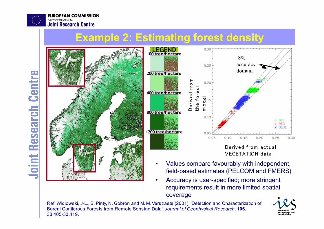
Example 2: Estimating forest density

!"#$%"&'(#)* '+,-.+/

0121343567'&+-+

!"#$%"&'(#)*

-8"'()#"9-

*)&"/

8%

accuracy

domain

Ref: Widlowski, J-L., B. Pinty, N. Gobron and M. M. Verstraete (2001) 'Detection and Characterization of

Boreal Coniferous Forests from Remote Sensing Data', Journal of Geophysical Research, 106,

33,405-33,419.

• Values compare favourably with independent,

field-based estimates (PELCOM and FMERS)

• Accuracy is user-specified; more stringent

requirements result in more limited spatial

coverage

200 tree/hectare

400 tree/hectare

800 tree/hectare

1200 tree/hectare

100 tree/hectareLEGEND



context


4. Applications

5. Exploiting RPV

Outline

Characterizing heterogeneity

Ref: Pinty, B. et al. (2002) 'Uniqueness of Multiangular Measurements, Part 1: An Indicator of Subpixel Surface

Heterogeneity from MISR', IEEE Transactions on Geoscience and Remote Sensing, MISR Special Issue, 40,

1560-1573.

3-D

Bell-shape

k=1.18

IPA

Bowl-shape

k=0.65

Overview of AirMISR

Ref: http://www-misr.jpl.nasa.gov/mission/minst.html.

• 1 camera pointable at ±70.5,±60, ±45.6, ±26.1, 0°

• Spectral bands at 446, 558,672, and 866 nm

• Spatial resolution: L1B2 data re-sampled at 27.5 m

• Image length: 9 – 26 km (0 –70°)

• Swath: 11 – 32 km (0 – 70°)

• Coverage: on request

• Data: LaRC DAAC

Atmospheric correction of AirMISR


SALINA, KS

July 1999

Top-of-atmosphere

Image (70º)

Rayleigh-corrected

Rayleigh + aerosol

corrected

Target structure and anisotropy (1)

Ref: Gobron, N. et al. (2002) 'Uniqueness of Multiangular Measurements, Part 2: Joint Retrieval of Vegetation

Structure and Photosynthetic Activity From MISR', IEEE Transactions on Geoscience and Remote Sensing,

MISR Special Issue, 40, 1574-1592.

1.5

1.0

0.5

Be

ll-sh

ap

eB

ow

l-sh

ap

ek

AirMISR campaign, Konza Prairie, June 1999


Ref: Gobron, N. et al. (2002) 'Uniqueness of Multiangular Measurements, Part 2: Joint Retrieval of Vegetation

Structure and Photosynthetic Activity From MISR', IEEE Transactions on Geoscience and Remote Sensing,

MISR Special Issue, 40, 1574-1592.

• Konza Prairie, June 2000

• A: Bare soil between trees

• B: Clearing between canopies

• C: Young corn field

• D: mixed vegetation

• E: Dry river bed

• F: Fence between two open

fields

• G: Agriculture

Overview of MISR


• 9 cameras at ±70.5, ±60, ±45.6,±26.1, 0°

• Each camera at 446, 558, 672,and 866 nm

• Spatial resolution: 275 m (250 mnadir)

• Global mode: Full res. nadir andred, 1.1 km otherwise

• Local mode: Full resolution allcameras and all bands

• Swath: 360 km

• Coverage: global (9 days)


Ref: http://www-misr.jpl.nasa.gov/gallery/galhistory/2001_may_30.html.

Saskatchewan

and Manitoba

April 17, 2001

RGB = Nir, R, G

285

km

RGB = R60a, Rn, R60f

N

Snow

Forests

Roads

Agriculture


Ref: http://www-misr.jpl.nasa.gov/gallery/galhistory.html

Saratov, Russia

31 May 2002 (top)

18 July 2002 (bottom)

‘True color’ MISR An (left)

Red anisotropy (right):

RGB = MISR Ca, An, Cf

Green: bell-shaped

anisotropy

controlled by soils and

vertical plants

Purple: bowl-shaped anisotropy

controlled by bare soils

Impact of Canopy Structure on surface BRF (1)

Ref: Widlowski, J.-L.et al. (2004) 'Canopy Structure Parameters Derived From Multi-angular Remote

Sensing Data for Terrestrial Carbon Studies', Climatic Change, 67, 403-415.

$=red

SZA=30°

IFOV~275 m

1.5

1.0

0.5

Bell shape

Bowl shape

kred

Impact of canopy structure on surface BRF (2)

Ref: Pinty, B.et al. (2002) 'Uniqueness of Multiangular Measurements Part 1: An Indicator of Subpixel Surface


1560-1573.

3-D

1-D

’

Leaf area index

(LAI) increases

The 1-D’ homologue of a 3-D

surface target features identical

optical (rL, tL, $soil), directional

(Bi-Lambertian) and structural

(LAI, LND, Lrad, LAD) canopy

characteristics as its 3-D original

with the exception of foliage

clumping.


Ref: Pinty, B.et al. (2002) 'Uniqueness of Multiangular Measurements Part 1: An Indicator of Subpixel Surface


1560-1573.

1-D! surface representations

(IPA) tend to be

characterized throughout

by bowl-shaped BRF fields

At low and high vegetation

coverage, 3-D scenes also

exhibit bowl-shaped BRF

fields

3-D scene representations

of intermediate vegetation

coverage tend to exhibit

bell-shaped reflectance

fields

3-D

1-D

’

k3-D ! k1-D’ if k3-D ! 1*


• It is not indifferent to use a 1D’ or a 3D model to represent theanisotropy of land surfaces.

• Detailed studies have been carried out to establish when 1D’models provide solutions equivalent to 3D models, and when 3Dmodels are absolutely required: See Widlowski et al. (2005) ‘Using1-D models to interpret the reflectance anisotropy of 3-D canopytargets: Issues and caveats’, IEEE TGRS, 43, 2008-2017.

• Using 3D models is particularly necessary to interpret remotesensing data at high spatial resolution; at coarse spatial resolutions(larger than a few hundred m), 1D’ models appear generallyadequate.

Documents

Information retrieval by explicit inversion - Earth Online¥act as common platform for intercomparison ¥document discrepancies between or uncertainties ... (1902): ¤ For each set