Embed Size (px)
Citation preview
JOURNAL OF GEOPHYSICAL RESEARCH: ATMOSPHERES, VOL. 118, 6869–6890, doi:10.1002/jgrd.50497, 2013
The fourth radiation transfer model intercomparison (RAMI-IV):Proficiency testing of canopy reflectance models with ISO-13528J.-L. Widlowski,1 B. Pinty,1 M. Lopatka,1 C. Atzberger,2 D. Buzica,3 M. Chelle,4M. Disney,5,6 J-P. Gastellu-Etchegorry,7 M. Gerboles,1 N. Gobron,1 E. Grau,7H. Huang,8 A. Kallel,9 H. Kobayashi,10,11 P. E. Lewis,5,6 W. Qin,12
M. Schlerf,13 J. Stuckens,14 and D. Xie15
Received 12 December 2012; revised 11 May 2013; accepted 13 May 2013; published 1 July 2013.
[1] The radiation transfer model intercomparison (RAMI) activity aims at assessing thereliability of physics-based radiative transfer (RT) models under controlled experimentalconditions. RAMI focuses on computer simulation models that mimic the interactions ofradiation with plant canopies. These models are increasingly used in the development ofsatellite retrieval algorithms for terrestrial essential climate variables (ECVs). Rather thanapplying ad hoc performance metrics, RAMI-IV makes use of existing ISO standards toenhance the rigor of its protocols evaluating the quality of RT models. ISO-13528 wasdeveloped “to determine the performance of individual laboratories for specific tests ormeasurements.” More specifically, it aims to guarantee that measurement results fallwithin specified tolerance criteria from a known reference. Of particular interest to RAMIis that ISO-13528 provides guidelines for comparisons where the true value of the targetquantity is unknown. In those cases, “truth” must be replaced by a reliable “conventionalreference value” to enable absolute performance tests. This contribution will show, forthe first time, how the ISO-13528 standard developed by the chemical and physicalmeasurement communities can be applied to proficiency testing of computer simulationmodels. Step by step, the pre-screening of data, the identification of reference solutions,and the choice of proficiency statistics will be discussed and illustrated with simulationresults from the RAMI-IV “abstract canopy” scenarios. Detailed performance statistics ofthe participating RT models will be provided and the role of the accuracy of the referencesolutions as well as the choice of the tolerance criteria will be highlighted.Citation: Widlowski, J.-L., et al. (2013), The fourth radiation transfer model intercomparison (RAMI-IV): Proficiency testing ofcanopy reflectance models with ISO-13528, J. Geophys. Res. Atmos., 118, 6869–6890, doi:10.1002/jgrd.50497.
1Institute for Environment and Sustainability, DG Joint ResearchCentre, European Commission, Ispra, Italy.
2Institute of Surveying, Remote Sensing and Land Information,University of Natural Resources and Life Sciences, Vienna, Austria.
3Industrial Emissions, Air Quality and Noise Unit, DG Environment,European Commission, Brussels, Belgium.
4Institut National de la Recherche Agronomique, Thiverval-Grignon,France.
5Department of Geography, University College London, UK.6Department of Meteorology, NERC National Centre for Earth
Observation (NCEO), University of Reading, Reading, UK.7Centre d’Etudes Spatiales de la BIOsphère, Toulouse, France.8Beijing Forestry University, Beijing, China.9Institut Supérieur d’Electronique et de Communication de Sfax,
Tunisia.10Department of Environmental Science, Policy and Management,
University of California, Berkeley, California, USA.11Japan Agency for Marine-Earth Science and Technology, Yokohama,
Japan.
Corresponding author: J.-L. Widlowski, Institute for Environment andSustainability, European Commission’s DG Joint Research Centre, TP272,I-21027 Ispra (VA), Italy. ([email protected])
©2013. American Geophysical Union. All Rights Reserved.2169-897X/13/10.1002/jgrd.50497
1. Introduction[2] Physics-based radiative transfer (RT) models simu-
late the interactions of solar radiation within a given medium(e.g., clouds, plant canopies, etc.). Increasingly, these mod-els contribute to the quantitative interpretation of remotesensing observations. Model simulations, for example, canbe used to generate look-up-tables, to train neural networks,or to develop parametric formulations that are then embed-ded in quantitative retrieval algorithms. A case in point aremany of the current LAI, FAPAR, and surface albedo prod-ucts that are derived from global medium-resolution sensors.The quality of RT models is thus essential if accurate andreliable information are to be derived from Earth Observa-tion (EO) data. In fact, the reliability of model simulations
12Science Systems and Applications, Inc., Greenbelt, Maryland, USA.13Département Environnement et Agro-biotechnologie, Centre de
Recherche Public - Gabriel Lippmann, Belvaux, Luxembourg.14Biosystems Department, Katholieke Universiteit Leuven, Leuven,
Belgium.15Research Center for Remote Sensing and GIS, School of Geography,
Beijing Normal University, Beijing, China.
6869
WIDLOWSKI ET AL.: RESULTS FOR RAMI-IV ABSTRACT CANOPIES
should at least be comparable to the space sensor uncer-tainties documented by vicarious calibration efforts. Thisis particularly so in the context of climate studies whereboth accuracy and stability requirements for satellite-derivedessential climate variables (ECVs) are increasingly stringent[GCOS, 2011].
[3] Obtaining accurate satellite and in situ estimates ofterrestrial ECVs is highly challenging. Most field valida-tion efforts of quantitative EO products over land are stillin a pre-standardized state. As such, it is not surprising thatneither funding agencies nor environmental legislation cur-rently enforces absolute quality criteria on satellite-derivedquantitative surface information. The situation is rather dif-ferent, however, when it comes to laboratory or in situ mea-surements in the field of environmental chemistry. Here alarge body of legislation exists at both national and suprana-tional level that (1) defines acceptable concentration rangesand limits of target substances, (2) regulates the manner inwhich these quantities should be measured and analysed, and(3) indicates procedures to deal with eventual exceedances.Fundamental to such a framework are both the availabilityof error-characterized reference methodologies and the exis-tence of standardized procedures allowing evaluation of thequality of alternative measurement techniques. Of particularinterest in this context is the formulation of methodologicalstandards that allow for regular testing of the proficiency oflaboratories. The goal of such procedures is to guarantee thatthe results—obtained by performing comparable analyseswith laboratory-specific measurement methods—fall withinspecified tolerance criteria from a known reference [Hundet al., 2000].
[4] Currently, the usage of these community-approvedand internationally applied quality assurance standards islimited to the evaluation of chemical and physical mea-surement procedures, e.g., Gerboles et al. [2011]. If itwere possible to apply these standards to the comparisonof physics-based computer simulation models (and subse-quently also satellite retrieval algorithms), then the rigorous-ness of such comparison efforts would certainly benefit, theirfindings would become more authoritative, and the accep-tance of their outcome would be broader. Such a transferof context appears feasible since the crux of absolute verifi-cation schemes remains essentially the same irrespective ofwhether one deals with measurements (i.e., laboratory or insitu data) or simulations (i.e., model or algorithm outputs).In both scenarios, the true value of the target quantity is gen-erally unknown, and thus, it is foremost the definition of areliable “conventional reference value” [JCGM, 2008] thatis required to carry out absolute performance tests. At thesame time, however, appropriate tolerance criteria must bedefined and suitable statistical tools selected to determinewhether a given bias is acceptable or not. In this contribu-tion, the international standard ISO 13528 [2005] (and inpart also ISO 5725-2 [1994]) is applied to the data sub-mitted to the fourth phase of the RAdiation transfer ModelIntercomparison (RAMI) exercise.
[5] As an open, self-organizing activity of the canopyRT modeling community the RAMI exercise has focused,since 1999, on the evaluation of models simulating bidirec-tional reflectance factors (BRFs) and radiative fluxes for 1-Dand 3-D vegetation canopies [Pinty et al., 2001, 2004]. Thefirst three phases of RAMI, which concentrated on relatively
simple and often abstracted plant environments, allowed par-ticipants to identify coding errors and to improve some ofthe RT formulations in their models. As such, model agree-ment increased and reached �1% on average among the3-D Monte Carlo models participating in the third phaseof RAMI [Widlowski et al., 2007b]. This in turn enabledthe definition of a “surrogate truth” data set and the sub-sequent development of a web-based benchmarking facil-ity known as the RAMI On-line Model Checker (ROMC)[Widlowski et al., 2007a]. “Credible” Monte Carlo modelsfrom RAMI-3 have also been used to evaluate the qualityof RT formulations embedded in the land surface schemesof soil-vegetation-atmosphere transfer (SVAT), numericalweather prediction (NWP), and global circulation models[Widlowski et al., 2011]. With these achievements, the scopeof RAMI was ready to be expanded toward more complexand realistic representations of plant environments as wellas the simulation of new types of measurements and remotesensing devices.
[6] This paper is subdivided as follows: Section 2 sum-marizes the experimental setup and measurement definitionsused by the fourth phase of RAMI (RAMI-IV). Section 3presents the outcome of several consistency checks that wereapplied to screen the contributions of the participating mod-els. Section 4 provides an overview of ISO-13528 and showshow this can be applied to define consensus reference valuesfor the RAMI-IV test cases. In section 5, the performanceof the participating models will be presented. Section 6concludes with a series of observations and remarks.
2. The Fourth Phase of RAMI[7] In February 2009, potential participants were invited
by email to contribute to RAMI-IV. A dedicated website(http://rami-benchmark.jrc.ec.europa.eu/) had been set upcontaining detailed descriptions of the prescribed test cases.Instructions were also provided as to what radiative quan-tities had to be simulated. The task of the participants thenconsisted in (1) representing the prescribed canopy architec-tures within their respective RT model(s), (2) executing theirmodels to simulate the prescribed radiation quantities underpredefined illumination and viewing conditions, and (3) for-matting and uploading the output of their models accordingto the RAMI specifications. Similar to previous phases ofRAMI the collection of results, their analysis, and any even-tual feedbacks to the model operators were carried out bythe European Commission’s Joint Research Centre (JRC) inIspra, Italy. Table 1 lists the models and operators that sub-mitted simulations for the abstract canopy experiments ofRAMI-IV.
2.1. RAMI-IV Abstract Canopies[8] Although RAMI-IV consisted of two separate sets of
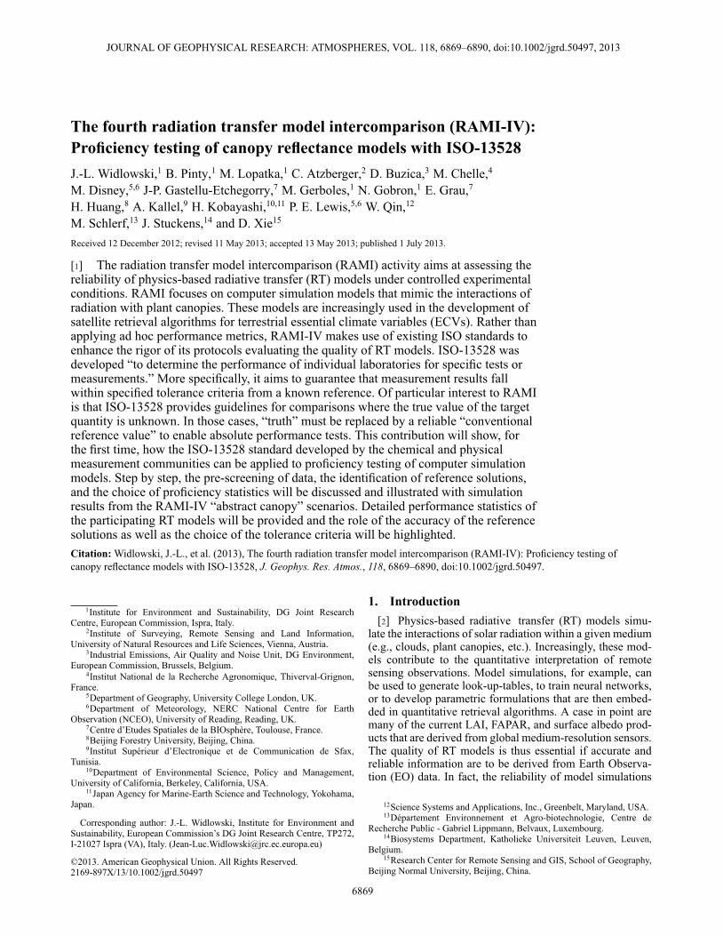
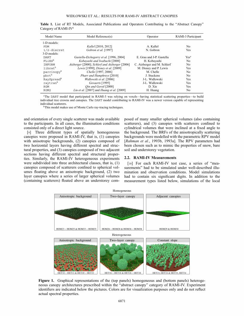
experiments only those pertaining to the “abstract canopy”category will be used in this work. Figure 1 provides agraphical overview of the prescribed architectural scenar-ios. As can be seen, the test cases were based exclusivelyon finite-sized disc-shaped scatterers (i.e., leaves) that werecharacterized by Lambertian scattering properties and vari-ous orientation distributions [Goel and Strebel, 1984]. Thescatterers were confined to spherical, cylindrical, or slab-like volumes floating above a flat background. The position
6870
WIDLOWSKI ET AL.: RESULTS FOR RAMI-IV ABSTRACT CANOPIES
Table 1. List of RT Models, Associated Publications and Operators Contributing to the “Abstract Canopy”Category of RAMI-IVa
Model Name Model Reference(s) Operator RAMI-3 Participant
1-D models:FDM Kallel [2010, 2012] A. Kallel No1/2-discret Gobron et al. [1997] N. Gobron Yes3-D models:DART Gastellu-Etchegorry et al. [1996, 2004] E. Grau and J-P. Gastellu Yesa
FLiESb Kobayashi and Iwabuchi [2008] H. Kobayashi NoINFORM Atzberger [2000]; Schlerf and Atzberger [2006] C. Atzberger and M. Schlerf Nolibratb Lewis [1999]; Disney et al. [2009] M. Disney and P. Lewis Yesparcinopyb Chelle [1997, 2006] M. Chelle Nopbrtb Pharr and Humphreys [2010] J. Stuckens NoRaySpreadb Widlowski et al. [2006] J-L. Widlowski Yesraytranb Govaerts [1995] J-L. Widlowski YesRGM Qin and Gerstl [2000] D. Xie YesRGM2 Liu et al. [2007] and Huang et al. [2009] H. Huang No
aThe DART model that participated in RAMI-3 was relying on voxels—having statistical scattering properties—to buildindividual tree crowns and canopies. The DART model contributing to RAMI-IV was a newer version capable of representingindividual scatterers.
bThis model makes use of Monte Carlo ray-tracing techniques.
and orientation of every single scatterer was made availableto the participants. In all cases, the illumination conditionsconsisted only of a direct light source.
[9] Three different types of spatially homogeneouscanopies were proposed in RAMI-IV, that is, (1) canopieswith anisotropic backgrounds, (2) canopies composed oftwo horizontal layers having different spectral and struc-tural properties, and (3) canopies composed of two adjacentsections having different spectral and structural proper-ties. Similarly, the RAMI-IV heterogeneous experimentswere subdivided into three architectural classes, that is, (1)canopies composed of scatterers confined to spherical vol-umes floating above an anisotropic background, (2) twolayer canopies where a series of larger spherical volumes(containing scatterers) floated above an understorey com-
posed of many smaller spherical volumes (also containingscatterers), and (3) canopies with scatterers confined tocylindrical volumes that were inclined at a fixed angle tothe background. The BRFs of the anisotropically scatteringbackgrounds were modelled with the parametric RPV model[Rahman et al., 1993b, 1993a]. The RPV parameters hadbeen chosen such as to mimic the properties of snow, baresoil and understorey vegetation.
2.2. RAMI-IV Measurements[10] For each RAMI-IV test case, a series of “mea-
surements” had to be simulated under well-described illu-mination and observation conditions. Model simulationshad to contain six significant digits. In addition to themeasurement types listed below, simulations of the local
Anisotropic background Two−layer canopy Adjacent canopies
Two−layer canopyAnisotropic background Constant slope
Homogeneous
Heterogeneous
HOM23 − HOM25 & HOM33 − HOM35 HOM26 − HOM28 & HOM36 − HOM38 HOM29 & HOM30
HET16 − HET18 & HET26 − HET28HET10 − HET12 & HET20 − HET22 HET23, HET24 & HET33, HET34
Figure 1. Graphical representations of the (top panels) homogeneous and (bottom panels) heteroge-neous canopy architectures prescribed within the “abstract canopy” category of RAMI-IV. Experimentidentifiers are indicated below the pictures. Colors are for visualization purposes only and do not reflectactual spectral properties.
6871
WIDLOWSKI ET AL.: RESULTS FOR RAMI-IV ABSTRACT CANOPIES
Table 2. Overview of the Type of Measurements Performed by RT Models Contributing to the “AbstractCanopy” Cases of RAMI-IVa
Model Name BRFs Fluxes Transmission Lidar
tot uc co mlt DHR fabs tot coco uc vprof loc_dir tot sgl
FDM X X X X X X X X X - - - -1/2-discret X X X X X X X X X - - - -DART X X X X X X X X X X - X XFLiES X X X X X X X X X X - X XINFORM X - - - - - - - - - - - -librat X X X X - - - X - - - X Xparcinopy X - - X X X X - X X - - -pbrt X X X X X Xb X X X X - - -rayspread X X X X - - - - - - X - -raytran - - - - X X X X X X - X XRGM X - - - - - - - - - - - -RGM2 X X X X X X X X X X - - XaBRF stands for bidirectional reflectance factor, uc for radiation uncollided with the vegetation, co for radiation
single-collided with vegetation, and mlt for multiple-collided radiation; tot is the contribution from all available radi-ation components, coco stands for radiation collided with the canopy only, sgl stands for radiation collided once witheither vegetation or background, DHR stands for directional hemispherical reflectance, fabs stands for fraction ofabsorbed radiation, vprof stands for vertical transmission profiles, and loc_dir stands for direct transmission at a par-ticular location within the canopy/scene.
bReconstructed by imposing energy conservation (�F = 0 in equation (1)) for test cases with Lambertianbackgrounds.
uncollided transmission along a transect at the lower bound-ary had been asked for. These simulations were intendedto mimic the radiative quantities that would be gathered bythe TRAC instrument [Chen and Cihlar, 1995] if placedwithin the heterogeneous abstract canopies of RAMI-IV.However, only the rayspread model submitted this type
of simulation results. Table 2 provides an overview ofthe contributions submitted by the various participatingRT models.2.2.1. Bi-Directional Reflectance Factors (BRFs)
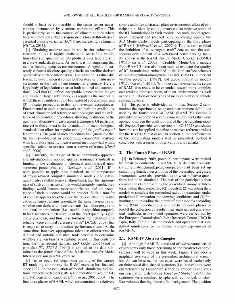
[11] BRFs had to be generated for view zenith angles at2° interval from ˙1ı to ˙75ı along the principal plane
tota
l BR
F
HET23_DIS_000_NIR_65 PP HET34_DIS_000_RED_50 PPHET24_DIS_180_NIR_05 OPHET21_DIS_UNI_NIR_20 PP
HOM34_DIS_ERE_NIR_20 OPHOM35_DIS_ERE_RED_20 OPHOM30_DIS_090_RED_50 OPHOM23_DIS_PLA_NIR_50 OP
tota
l BR
F
sing
le c
ollid
ed B
RF
sing
le u
ncol
lided
BR
F
sing
le c
ollid
ed B
RF
mul
tiple
sca
ttere
d B
RF
mul
tiple
sca
ttere
d B
RF
sing
le u
ncol
lided
BR
F
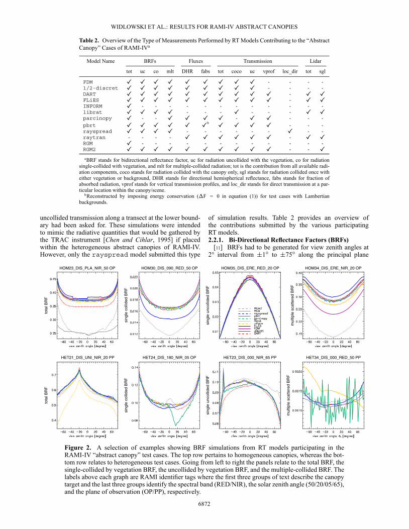
Figure 2. A selection of examples showing BRF simulations from RT models participating in theRAMI-IV “abstract canopy” test cases. The top row pertains to homogeneous canopies, whereas the bot-tom row relates to heterogeneous test cases. Going from left to right the panels relate to the total BRF, thesingle-collided by vegetation BRF, the uncollided by vegetation BRF, and the multiple-collided BRF. Thelabels above each graph are RAMI identifier tags where the first three groups of text describe the canopytarget and the last three groups identify the spectral band (RED/NIR), the solar zenith angle (50/20/05/65),and the plane of observation (OP/PP), respectively.
6872
WIDLOWSKI ET AL.: RESULTS FOR RAMI-IV ABSTRACT CANOPIES
raytran
parcinopy
pbrt
FLiES
DART
RGM−2
downward flux
heig
ht [m
]
heig
ht [m
]
upward flux
heig
ht [m
]
upward flux
downward flux
heig
ht [m
]
lidar return profiles
return signal (arbitrary units)
return signal (arbitrary units) return signal (arbitrary units)
vertical transmission profiles
heig
ht [m
]
heig
ht [m
]
heig
ht [m
]
heig
ht [m
]
return signal (arbitrary units)
librat
raytran
RGM−2
DART
FLiES
single scattering only
single scattering only total contribution
total contribution
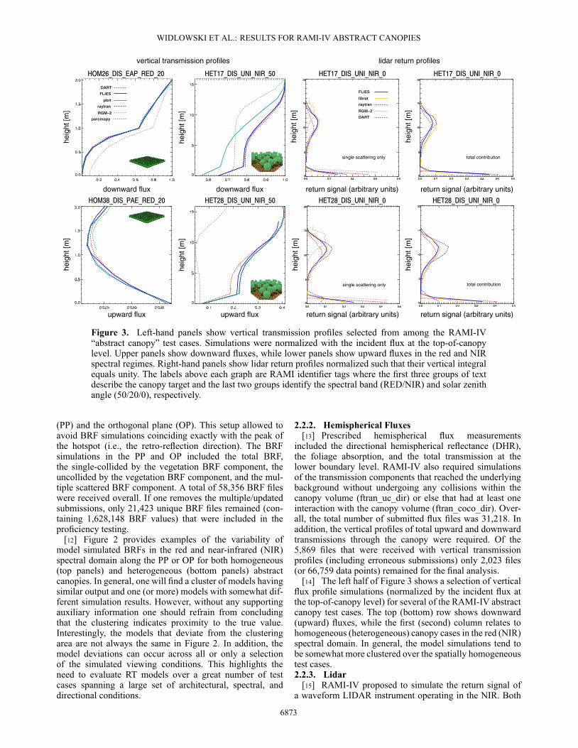
Figure 3. Left-hand panels show vertical transmission profiles selected from among the RAMI-IV“abstract canopy” test cases. Simulations were normalized with the incident flux at the top-of-canopylevel. Upper panels show downward fluxes, while lower panels show upward fluxes in the red and NIRspectral regimes. Right-hand panels show lidar return profiles normalized such that their vertical integralequals unity. The labels above each graph are RAMI identifier tags where the first three groups of textdescribe the canopy target and the last two groups identify the spectral band (RED/NIR) and solar zenithangle (50/20/0), respectively.
(PP) and the orthogonal plane (OP). This setup allowed toavoid BRF simulations coinciding exactly with the peak ofthe hotspot (i.e., the retro-reflection direction). The BRFsimulations in the PP and OP included the total BRF,the single-collided by the vegetation BRF component, theuncollided by the vegetation BRF component, and the mul-tiple scattered BRF component. A total of 58,356 BRF fileswere received overall. If one removes the multiple/updatedsubmissions, only 21,423 unique BRF files remained (con-taining 1,628,148 BRF values) that were included in theproficiency testing.
[12] Figure 2 provides examples of the variability ofmodel simulated BRFs in the red and near-infrared (NIR)spectral domain along the PP or OP for both homogeneous(top panels) and heterogeneous (bottom panels) abstractcanopies. In general, one will find a cluster of models havingsimilar output and one (or more) models with somewhat dif-ferent simulation results. However, without any supportingauxiliary information one should refrain from concludingthat the clustering indicates proximity to the true value.Interestingly, the models that deviate from the clusteringarea are not always the same in Figure 2. In addition, themodel deviations can occur across all or only a selectionof the simulated viewing conditions. This highlights theneed to evaluate RT models over a great number of testcases spanning a large set of architectural, spectral, anddirectional conditions.
2.2.2. Hemispherical Fluxes[13] Prescribed hemispherical flux measurements
included the directional hemispherical reflectance (DHR),the foliage absorption, and the total transmission at thelower boundary level. RAMI-IV also required simulationsof the transmission components that reached the underlyingbackground without undergoing any collisions within thecanopy volume (ftran_uc_dir) or else that had at least oneinteraction with the canopy volume (ftran_coco_dir). Over-all, the total number of submitted flux files was 31,218. Inaddition, the vertical profiles of total upward and downwardtransmissions through the canopy were required. Of the5,869 files that were received with vertical transmissionprofiles (including erroneous submissions) only 2,023 files(or 66,759 data points) remained for the final analysis.
[14] The left half of Figure 3 shows a selection of verticalflux profile simulations (normalized by the incident flux atthe top-of-canopy level) for several of the RAMI-IV abstractcanopy test cases. The top (bottom) row shows downward(upward) fluxes, while the first (second) column relates tohomogeneous (heterogeneous) canopy cases in the red (NIR)spectral domain. In general, the model simulations tend tobe somewhat more clustered over the spatially homogeneoustest cases.2.2.3. Lidar
[15] RAMI-IV proposed to simulate the return signal ofa waveform LIDAR instrument operating in the NIR. Both
6873
WIDLOWSKI ET AL.: RESULTS FOR RAMI-IV ABSTRACT CANOPIES
the total return signal and that accounting for the first orderof scattering in the canopy had to be generated. More specif-ically, the models should mimic an instantaneous pulse ofradiation that resulted in a circular footprint of 50 m diameterat the top-of-canopy height level. Only photons exiting fromthis uniformly illuminated target area could actually con-tribute to the lidar return signal. The waveform signal itselfwas to be discretised into contributions originating from 20height intervals/bins of equal thickness. The field of view(FOV) of the detector was set to 24 mrad, and its heightwas equal to 2000 m (above the background). The radius ofthe telescope collecting the returned photons was 1 m. Theactual quantity to report was the amount of radiation thatwas scattered back up from a given height interval/bin intothe field of view of the detector normalized by the incidentradiation within the footprint area.
[16] The definition of the lidar measurements in RAMI-IVlead to different interpretations of the target quantities. Assuch, the results displayed in the right half of Figure 3 werenormalized for better visual comparison in a manner suchthat the sum of contributions from all height intervals/binsequals unity. The rightmost panels show the total return sig-nal, whereas the inner panels show the return signal afterone scattering event. Although the exact lidar profiles aresomewhat different, the peak of their overstory contributionoccurs at very similar heights. This is especially the casefor the FLiES, librat, and raytran models. Due to thedifferences in the formats of the received data set, it wasdecided not to pursue their analysis further at this stage butto refine the simulation requirements on the RAMI websitefirst.
3. Model Consistency Checks[17] In line with the requirements of ISO-13528 and also
in analogy to previous phases of RAMI, a series of modelconsistency checks were carried out prior to the actualproficiency testing.
3.1. Energy Conservation[18] Energy conservation describes the fact that all radia-
tion entering or exiting a given plant canopy volume must bein balance with the amount of energy that is being absorbedby this volume. In RAMI-IV, energy conservation can onlybe evaluated for test cases having backgrounds with Lam-bertian scattering properties. In those cases, the deviationof model m from energy conservation for any particularstructural (�), spectral (�) and illumination (�i) relatedconditions, can be defined as
�Fm(�, �,�i) = 1 – [Am(�, �,�i) + Rm(�, �,�i)+ (1 – ˛(�, �,�i)) � Tm(�, �,�i) ] (1)
where the hemispherical fluxes A, R, and T relate to thefoliage absorption, black sky albedo, and canopy transmis-sion measurements, respectively (given that no wood waspresent in the abstract canopy scenes). The backgroundalbedo, denoted here by ˛, was provided on the RAMI web-site. The overall deviation from energy conservation can bedefined as the arithmetic average over a series of selectedcases:
�Fm =1
NF(m)
Nm�X�=1
Nm�X�=1
Nm�iX
i=1
�Fm(�, �, i)
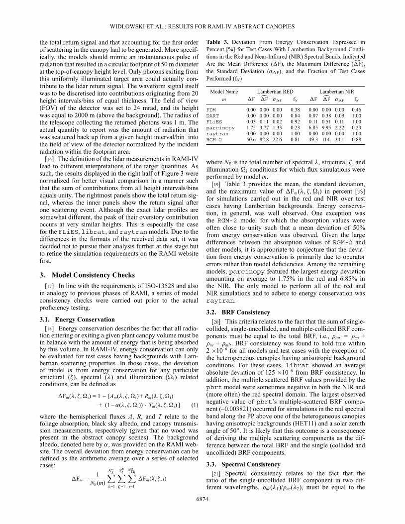
Table 3. Deviation From Energy Conservation Expressed inPercent [%] for Test Cases With Lambertian Background Condi-tions in the Red and Near-Infrared (NIR) Spectral Bands. IndicatedAre the Mean Difference (�F), the Maximum Difference (c�F),the Standard Deviation (��F), and the Fraction of Test CasesPerformed (fN)
Model Name Lambertian RED Lambertian NIRm �F c�F ��F fN �F c�F ��F fN
FDM 0.00 0.00 0.00 0.38 0.00 0.00 0.00 0.46DART 0.00 0.00 0.00 0.84 0.07 0.38 0.09 1.00FLiES 0.03 0.11 0.02 0.92 0.11 0.51 0.11 1.00parcinopy 1.75 3.77 1.33 0.23 6.85 9.95 2.22 0.23raytran 0.00 0.00 0.00 1.00 0.00 0.00 0.00 1.00RGM-2 50.6 82.8 22.6 0.81 49.3 114. 34.1 0.88
where NF is the total number of spectral �, structural �, andillumination �i conditions for which flux simulations wereperformed by model m.
[19] Table 3 provides the mean, the standard deviation,and the maximum value of �Fm(�, �,�i) in percent [%]for simulations carried out in the red and NIR over testcases having Lambertian backgrounds. Energy conserva-tion, in general, was well observed. One exception wasthe RGM-2 model for which the absorption values wereoften close to unity such that a mean deviation of 50%from energy conservation was observed. Given the largedifferences between the absorption values of RGM-2 andother models, it is appropriate to conjecture that the devia-tion from energy conservation is primarily due to operatorerrors rather than model deficiencies. Among the remainingmodels, parcinopy featured the largest energy deviationamounting on average to 1.75% in the red and 6.85% inthe NIR. The only model to perform all of the red andNIR simulations and to adhere to energy conservation wasraytran.
3.2. BRF Consistency[20] This criteria relates to the fact that the sum of single-
collided, single-uncollided, and multiple-collided BRF com-ponents must be equal to the total BRF, i.e., �tot = �co +�uc + �mlt. BRF consistency was found to hold true within2 �10–6 for all models and test cases with the exception ofthe heterogeneous canopies having anisotropic backgroundconditions. For these cases, librat showed an averageabsolute deviation of 125 �10–6 from BRF consistency. Inaddition, the multiple scattered BRF values provided by thepbrt model were sometimes negative in both the NIR and(more often) the red spectral domain. The largest observednegative value of pbrt’s multiple-scattered BRF compo-nent (–0.003821) occurred for simulations in the red spectralband along the PP above one of the heterogeneous canopieshaving anisotropic backgrounds (HET11) and a solar zenithangle of 50ı. It is likely that this outcome is a consequenceof deriving the multiple scattering components as the dif-ference between the total BRF and the single (collided anduncollided) BRF components.
3.3. Spectral Consistency[21] Spectral consistency relates to the fact that the
ratio of the single-uncollided BRF component in two dif-ferent wavelengths, �uc(�1)/�uc(�2), must be equal to the
6874
WIDLOWSKI ET AL.: RESULTS FOR RAMI-IV ABSTRACT CANOPIES
spec
tral
con
sist
ency
dev
iatio
n
view zenth angle [degree] view zenth angle [degree] view zenth angle [degree]
view zenth angle [degree]view zenth angle [degree]view zenth angle [degree]
spec
tral
con
sist
ency
dev
iatio
n
spec
tral
con
sist
ency
dev
iatio
nsp
ectr
al c
onsi
sten
cy d
evia
tion
spec
tral
con
sist
ency
dev
iatio
nsp
ectr
al c
onsi
sten
cy d
evia
tion
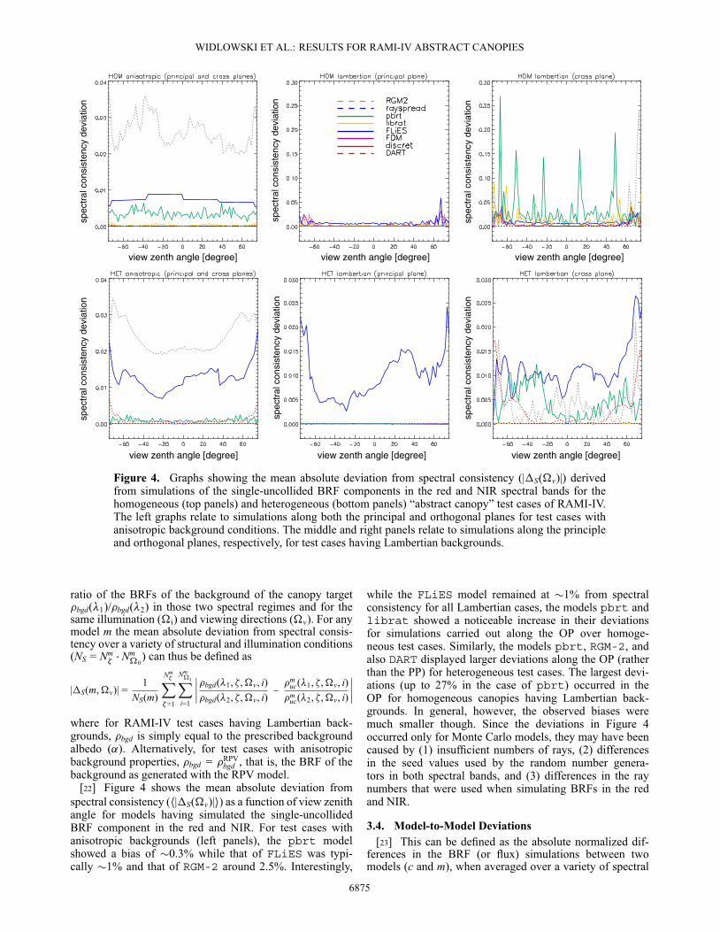
Figure 4. Graphs showing the mean absolute deviation from spectral consistency (|�S(�v)|) derivedfrom simulations of the single-uncollided BRF components in the red and NIR spectral bands for thehomogeneous (top panels) and heterogeneous (bottom panels) “abstract canopy” test cases of RAMI-IV.The left graphs relate to simulations along both the principal and orthogonal planes for test cases withanisotropic background conditions. The middle and right panels relate to simulations along the principleand orthogonal planes, respectively, for test cases having Lambertian backgrounds.
ratio of the BRFs of the background of the canopy target�bgd(�1)/�bgd(�2) in those two spectral regimes and for thesame illumination (�i) and viewing directions (�v). For anymodel m the mean absolute deviation from spectral consis-tency over a variety of structural and illumination conditions(NS = Nm
�� Nm�0
) can thus be defined as
|�S(m,�v)| =1
NS(m)
Nm�X�=1
Nm�iX
i=1
ˇ̌̌̌�bgd(�1, �,�v, i)�bgd(�2, �,�v, i)
–�m
uc(�1, �,�v, i)�m
uc(�2, �,�v, i)
ˇ̌̌̌where for RAMI-IV test cases having Lambertian back-grounds, �bgd is simply equal to the prescribed backgroundalbedo (˛). Alternatively, for test cases with anisotropicbackground properties, �bgd = �RPV
bgd , that is, the BRF of thebackground as generated with the RPV model.
[22] Figure 4 shows the mean absolute deviation fromspectral consistency (h|�S(�v)|i) as a function of view zenithangle for models having simulated the single-uncollidedBRF component in the red and NIR. For test cases withanisotropic backgrounds (left panels), the pbrt modelshowed a bias of �0.3% while that of FLiES was typi-cally �1% and that of RGM-2 around 2.5%. Interestingly,
while the FLiES model remained at �1% from spectralconsistency for all Lambertian cases, the models pbrt andlibrat showed a noticeable increase in their deviationsfor simulations carried out along the OP over homoge-neous test cases. Similarly, the models pbrt, RGM-2, andalso DART displayed larger deviations along the OP (ratherthan the PP) for heterogeneous test cases. The largest devi-ations (up to 27% in the case of pbrt) occurred in theOP for homogeneous canopies having Lambertian back-grounds. In general, however, the observed biases weremuch smaller though. Since the deviations in Figure 4occurred only for Monte Carlo models, they may have beencaused by (1) insufficient numbers of rays, (2) differencesin the seed values used by the random number genera-tors in both spectral bands, and (3) differences in the raynumbers that were used when simulating BRFs in the redand NIR.
3.4. Model-to-Model Deviations[23] This can be defined as the absolute normalized dif-
ferences in the BRF (or flux) simulations between twomodels (c and m), when averaged over a variety of spectral
6875
WIDLOWSKI ET AL.: RESULTS FOR RAMI-IV ABSTRACT CANOPIES
RG
M−
2
RG
M
Ray
Spre
ad
pbrt
libra
t
FLiE
S
FDM
disc
ret
parc
inop
yD
AR
T
RG
M−
2
RG
M
Ray
Spre
ad
pbrt
libra
t
FLiE
S
FDM
disc
ret
parc
inop
yD
AR
T
RG
M−
2
RG
M
Ray
Spre
ad
pbrt
libra
t
FLiE
S
FDM
disc
ret
parc
inop
yD
AR
T
parcinopy
DART
discret
FDM
FLiES
librat
pbrt
RaySpread
RGM
RGM−2
RGM−2
RaySpread
pbrt
libratFLiES
DART
inform
RG
M−
2R
aySp
read
pbrt
libra
t
FLiE
S
info
rm
DA
RT
RG
M−
2R
aySp
read
pbrt
libra
t
FLiE
S
info
rm
DA
RT
RG
M−
2R
aySp
read
pbrt
libra
t
FLiE
S
info
rm
DA
RT
RG
M−
2R
aySp
read
pbrt
libra
t
FLiE
S
info
rm
DA
RT
RG
M−
2
rayt
ran
pbrt
parc
inop
y
FLiE
S
FDM
disc
ret
DA
RT
RG
M−
2
rayt
ran
pbrt
parc
inop
y
FLiE
S
FDM
disc
ret
DA
RT
RG
M−
2
rayt
ran
pbrt
parc
inop
y
FLiE
S
FDM
disc
ret
DA
RT
RG
M−
2
rayt
ran
pbrt
parc
inop
y
FLiE
S
FDM
disc
ret
DA
RT
RG
M−
2
rayt
ran
pbrt
parc
inop
y
FLiE
S
FDM
disc
ret
DA
RT
RGM−2
raytran
pbrt
parcinopyFLiES
FDM
DARTdiscret
total
RG
M−
2
RG
M
Ray
Spre
ad
pbrt
libra
t
FLiE
S
FDM
disc
ret
parc
inop
yD
AR
T
BRF quantities (heterogeneous cases)
BRF quantities (homogeneous cases)
ftran_uc_dir ftran_coco_dir
flux quantities (all cases)
single−collided single−uncollided multiple−collided
uncollidedtotal single−collided multiple−collided
transmissionabsorptioncanopy albedo
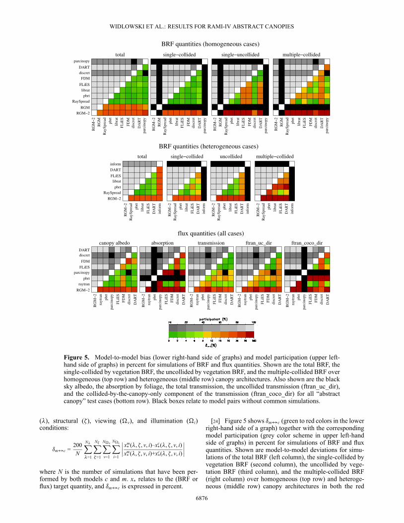
Figure 5. Model-to-model bias (lower right-hand side of graphs) and model participation (upper left-hand side of graphs) in percent for simulations of BRF and flux quantities. Shown are the total BRF, thesingle-collided by vegetation BRF, the uncollided by vegetation BRF, and the multiple-collided BRF overhomogeneous (top row) and heterogeneous (middle row) canopy architectures. Also shown are the blacksky albedo, the absorption by foliage, the total transmission, the uncollided transmission (ftran_uc_dir),and the collided-by-the-canopy-only component of the transmission (ftran_coco_dir) for all “abstractcanopy” test cases (bottom row). Black boxes relate to model pairs without common simulations.
(�), structural (�), viewing (�v), and illumination (�i)conditions:
ım$c =200N
N�X�=1
N�X�=1
N�vXv=1
N�iXi=1
ˇ̌̌̌xm
* (�, �, v, i)–xc*(�, �, v, i)
xm* (�, �, v, i)+xc
*(�, �, v, i)
ˇ̌̌̌
where N is the number of simulations that have been per-formed by both models c and m. x* relates to the (BRF orflux) target quantity, and ım$c is expressed in percent.
[24] Figure 5 shows ım$c (green to red colors in the lowerright-hand side of a graph) together with the correspondingmodel participation (grey color scheme in upper left-handside of graphs) in percent for simulations of BRF and fluxquantities. Shown are model-to-model deviations for simu-lations of the total BRF (left column), the single-collided byvegetation BRF (second column), the uncollided by vege-tation BRF (third column), and the multiple-collided BRF(right column) over homogeneous (top row) and heteroge-neous (middle row) canopy architectures in both the red
6876
WIDLOWSKI ET AL.: RESULTS FOR RAMI-IV ABSTRACT CANOPIES
and NIR spectral regimes. Black boxes relate to model pairsthat do not have any simulations in common. Note that theresults are normalized with respect to the number of BRFsimulations that were carried out by a given pair of models.
[25] Mean absolute model-to-model BRF differences (topleft panel) indicate a generally good agreement (ım$c < 6%)between all of the participants apart from RGM and RGM-2.The latter two models stand somewhat apart for the totalBRF simulations and, at least in the case of RGM-2, also forthe various BRF components. This pattern is independent ofthe spectral band (not shown) or canopy scenario (althoughıRGM-2$c was less than 20% for the single-uncollided com-ponent over test cases with an anisotropic background aswell as for the single-collided BRF component over the twolayer canopy test cases). During RAMI-3, the RGM modeldelivered total BRF simulations for homogeneous canopiesthat did not deviate by more than a couple of percent fromthe majority of participating models. Given the radiositynature of the RGMmodel, this could suggest that the observeddifferences in RAMI-IV are likely due to operator errors inthe implementation of the new test cases. In fact, it turnedout that the RGM-2 model simulations were based on archi-tectural scenarios that differed from those prescribed onthe RAMI website. For example, square leaves were usedfor the homogeneous test cases, a single spherical entitywas used for the heterogeneous test cases instead of sev-eral thousand discs, and spatially reduced versions of thescenes were regularly used to save computing time. Sincecanopies are replicated indefinitely in these models, the lattersimplification may have lead to artificial patterns of objectarrangements (for the heterogeneous canopies) with subse-quent biases in the simulated RT properties. This togetherwith possible operator errors in the assigning of spectralcanopy properties or the scaling of model-simulated radia-tive quantities may be the actual reasons for the observedbiases of RGM-2.
[26] The models FLiES, FDM, and DART show deviationsof up to 20% for the uncollided BRF component. At leastfor the DART model, this bias is very similar to that of theDART model participating in RAMI-3 (see Figure 6 in Wid-lowski et al. [2007b]). The large model-to-model differencesof these three models may be affected by the very low uncol-lided BRF values of the HOM26/HOM36 two-layer canopycases (�uc < 10–5 at large view zenith angles). In these sce-narios, small differences in model simulations (for example,due to Monte Carlo noise) may strongly affect the valueof ım$c. Model-to-model deviations generally increased forthe multiple-collided BRF component and in particular soin the red spectral domain (not shown) due to the smallerBRF values there. Whereas the noise in the Monte Carlosimulations of pbrt (compare with the leftmost lower panelin Figure 2) could explain its increased ım$c values, theFLiES and DART model simulations are not affected bynoisy BRF signals yet they were found to differ from othermodels in the NIR (not shown). This was particularly so overhomogeneous adjacent canopies and for canopies with ananisotropic background.
[27] Fewer models participated in the heterogeneous testcases of RAMI-IV. Again, the RGM-2 model is consistentlydifferent from other models here. The total BRF simulationsof the inform model are also different from those of otherRT models. DART simulations become increasingly different
when going from the single-collided to the single-uncollidedand finally to the multiple-collided BRF components. Thebias of the uncollided BRF component arises from simula-tions pertaining to the constant slope and two-layer canopycases in both the red and NIR. For the multiple-collided BRFsimulations, it is again the simulations in the red spectralband (not shown) that lead to the largest deviations.
[28] The final row in Figure 5 shows the average model-to-model bias for the black sky albedo, the absorption byfoliage, the total transmission, the uncollided transmission(ftran_uc_dir), and the collided-by-the-canopy-only compo-nent of the transmission (ftran_coco_dir). Whereas mostmodels agree for simulations of the canopy albedo andtransmission, this is no longer the case for the foliageabsorption and the collided-by-the-canopy-only componentof the transmitted flux. In particular, the discret andparcinopy models seem to differ in their canopy absorp-tion estimates, whereas the pbrt and discret modelsstand relatively apart in their ftran_coco_dir simulations.4. Proficiency Testing for RT Models
[29] The purpose of proficiency testing as described byISO-13528 is “to demonstrate that the measurement resultsobtained by laboratories do not exhibit evidence of an unac-ceptable level of bias.” The focus is thus not only on the“measurement”—which relates to the output of an instru-ment in response to external stimuli—but rather on theoverall “method” that is used to obtain the measurementresults. In general, the accuracy of the measurement methodwill depend on (1) the acquisition/preparation of the sam-ple, (2) the appropriateness of the instrument’s technology todeliver accurate results irrespective of the conditions underwhich the sample was acquired and subsequently analyzed,and (3) the choices/expertise of the operator carrying out thework (in a particular laboratory/outdoor environment).
[30] By analogy, the focus of RAMI is not only onthe “simulation”—which relates to the output of a modelin response to external inputs—but rather on the overall“method” that is used to generate the simulation results. Ingeneral, the accuracy of a simulation method depends on (1)the abstraction/representation of the target, (2) the appropri-ateness of the model’s mathematical formulations to deliveraccurate results irrespective of the nature of the target andthe external forcings, and (3) the choices/expertise of theoperator carrying out the work (in a particular computinglanguage/environment). The purpose of using ISO-13528 inthe context of RAMI is thus to demonstrate that the simu-lation results obtained by models do not exhibit evidence ofan unacceptable level of bias.
4.1. Applying ISO-13528 to Canopy RT Models[31] The following list describes how the various
steps prescribed by ISO-13528 for inter-laboratoryproficiency testing were implemented in the context ofRAMI-IV:
[32] 1. Ensure the homogeneity and stability of thesamples that are to be analyzed by the participants. Theseissues, while being relevant for interlaboratory proficiencytests, are essentially absent when it comes to RT model inter-comparisons. This is so because the samples (called testcases in RAMI) are virtual and their characteristics are avail-able in an exact, deterministic, and identical manner to all
6877
WIDLOWSKI ET AL.: RESULTS FOR RAMI-IV ABSTRACT CANOPIES
RAMI-IV participants via the relevant webpages. It shouldbe noted here that the RAMI coordinators have made everypossible effort to provide detailed and accurate descriptionsof the test cases and their associated measurement types.Should a model not be able to generate an exact copy ofa RAMI test case, then this cannot be a limitation of thesample (i.e., the test cases provided on the RAMI website)but rather due to the model’s internal RT formalism and/orthe operator’s choices when transferring the prescribed testcase characteristics to the model. Although feasible, noefforts were undertaken in this phase of RAMI to randomizeoperator effects.
[33] 2. Assign a reference value against which the biasof the participants can be determined. Ideally, this assignedreference value (X) should come with a standard uncertainty(uX) and be as close as possible to the true value of thequantity under study (here BRFs and hemispherically inte-grated radiative fluxes). In cases like RAMI where it is notpossible to determine X and uX prior to the launch of themodel intercomparison exercise, ISO-13528 recommends touse consensus values derived either from the simulations ofselected expert models or else from the participants of theproficiency test itself. These approaches are pursued hereand described in greater detail in section 4.2.
[34] 3. Specify a tolerance criteria allowing to determinewhether deviations from the reference are significant. Manyevaluation metrics proposed by ISO-13528 include a mea-sure of the bias levels that are still tolerable. For RAMI-IV,this “standard deviation of the proficiency assessment” ( O�)as it is called in ISO-13528 was prescribed in different waysdepending on the radiative quantity of interest. For BRFquantities, it was expressed as a fixed fraction (f) of thereference (X):
O��* = f � X�*
where the value of f was set to 0.03 and 0.05 in accordancewith the 3–5% error margins obtained by vicarious calibra-tion efforts of space borne remote sensing devices in thevisible and NIR, e.g., Thome [2001], Bruegge et al. [2002],Kneubühler et al. [2002], Thome et al. [2008], and Wanget al. [2011].
[35] The proficiency standard deviation for canopy albedo(R) and foliage absorption (A) was defined using themaximum tolerable bias specified by the Global ClimateObserving System (GCOS) in its satellite supplement to theimplementation plan [GCOS, 2011]:
O�R = 0.05 � XR/p
3 if 0.05 � XR > 0.0025= 0.0025/
p3 otherwise
O�A = 0.10 � XA/p
3 if 0.10 � XA > 0.05= 0.05/
p3 otherwise
where XR and XA are the reference values for the canopyalbedo and foliage absorption, respectively, and the
p3 fac-
tor arises from the (type B) rectangular distribution that wasassumed in accordance with section 4.4 of JCGM [2008]for biases falling within the range tolerated by GCOS. Sincecanopy transmission is not an “essential climate variable”GCOS does not provide a corresponding tolerance criteria.However, if one assumes zero correlation between the vari-ous terms in the energy balance equation (equation (1)), then
a proficiency standard deviation for T can be estimated onthe basis of the GCOS accuracy criteria for A and R:
O�T �
sO�2
R + O�2A
(1 – Rbgd)2 +(1 – XR – XA)2
(1 – Rbgd)4 � O�2Rbgd
For RAMI, the contribution from the background albedo iseither zero (because Rbgd = ˛ is prescribed for Lamber-tian backgrounds) or else very small (numerical integrationof RPV model). Hence, only the first term in the aboveequation was used to estimate O�T. The resulting values ofO�T were found to lie between 0.033 and 0.105 (mean value= 0.042) with little differences between the red and NIRspectral domain. To place this into perspective, the assignedreference values of the canopy transmission varied from0.007 (0.205) to 0.885 (0.959) in the red (NIR) with an aver-age value of 0.452 (0.676) over all abstract canopy cases inRAMI-IV.
[36] By setting the O� requirements in this manner, theproficiency assessment becomes equivalent to a “fitnessfor purpose” statement of the participating models, namely,whether they can simulate BRFs within the accuracies cur-rently achieved by vicarious calibration efforts of satelliteobservations and whether they can match the GCOS accu-racy criteria for canopy albedo and the fraction of absorbedradiation (FAPAR).
[37] 4. Compare the uncertainty of the assigned referencevalue (uX) with the tolerable deviation for the proficiencyassessment ( O�). ISO-13528 states that when uX � 0.3 � O� ,then the uncertainty of the assigned value is negligible andneed not be included in interpretation efforts of the pro-ficiency test [ISO 13528, 2005]. More specifically, if theabove criteria are satisfied, then a simple z-score metric willsuffice to assess model proficiency, while in cases where thestandard uncertainty of the reference exceeds 0.3 � O� , thenz0-scores will have to be used as described in section 5.3.The actual computation of uX is detailed in Appendix A andsections 4.2.3 and 4.2.4.
[38] If the standard deviation of the proficiency assess-ment ( O�) was assumed to be 3% (5%) of the assignedreference value, then the standard uncertainty of the assignedvalue was negligible in only 11.0% (26.7%) of the cases forthe multiple-collided BRF component. At the same time, uXwas negligible for 87.8% (91.2%) of the single-uncollidedBRFs, 99.2% (�100%) of the single-collided BRFs, and71.2% (86.8%) of the total BRF simulations. Canopy struc-ture affected the results for uncollided BRFs, while spectralbands affected those for multiple-collided and total BRFs.As such, uX was negligible in only 51.4% (61.7%) ofthe uncollided BRF simulations pertaining to homogeneoustwo-layer canopies, whereas this fraction increased to almost100% for heterogeneous canopies with anisotropic back-grounds if f = 0.03 (0.05). Similarly, the percentage of caseswhere uX for the multiple-collided BRF component wascompliant with the above ISO criteria changed from 1.5%(7.1%) for homogeneous canopies with anisotropic back-grounds to 34.7% (67.4%) for the homogeneous two layertest cases.
[39] For simulations of the canopy albedo, it turned outthat the above uXR � 0.3 � O�R condition was satisfied onaverage for 59.7% of all cases. For canopy absorption, thecompliance rate lay at 79.4%, while for transmission it was
6878
WIDLOWSKI ET AL.: RESULTS FOR RAMI-IV ABSTRACT CANOPIES
78.3%. Results varied somewhat between test cases withthe homogeneous two-layer canopy always delivering thebest compliance (at almost 100%) while the heterogeneoustwo-layer cases had the least compliances, that is, 34.2%for R, 47.5% for A, and 51.7% for T. Overall, these resultsthus suggested that it is prudent to include the uncertaintyof the assigned reference values in the data analysis stepand to base any performance statistics on z0-scores ratherthan z scores.
[40] 5. Evaluate the number of replicate simulations sothat the repeatability standard deviation (�r) is negligiblewith respect to the tolerable deviation for the proficiencyassessment ( O�). Repeatability is defined here in analogy withits measurement counterpart in JCGM [2008], that is, as “thecloseness of the agreement between the results of successivesimulations of the same quantity carried out under identi-cal conditions.” ISO 13528 requires �r/
pn � 0.3 O� in order
to eliminate the risk that repeatability variations cause theresults of the proficiency test to be erratic (here n is the num-ber of replicates). When it comes to physically based RTmodels, replicate simulations are rarely carried out. This iseither due to the large computing times required to do soor because the majority of model classes identified by Goel[1988] delivers invariant simulation results for a given setof input values (assuming the computing environment is notmodified between runs). Thus, �r = 0 for most RT mod-els and the above ISO-13528 criteria is always satisfied.The sole exception to this comes from “Monte Carlo” (MC)ray-tracing models where convergence toward a solution isachieved at a rate proportional to the inverse square root ofthe number of rays that are used to stochastically samplethe probability density function characterizing the scatteringbehavior of the canopy system under study [Disney et al.,2000]. Conceptually, the repeatability of the simulations ofa MC model will depend on (1) the number of rays that areused, (2) the seed number determining the locations of theincident rays above the target, (3) the architectural and spec-tral complexity of the system under study, and (4) the choiceand degree of variance reduction techniques.
[41] The repeatability of MC ray-tracing models couldnot be determined using the “balanced uniform-level” exper-iments described in ISO 5725-2 [1994] because a portingof MC models (acting as the “method” to be evaluated)to different computing environments (acting as “laborato-ries” here) was beyond the scope of RAMI-IV. Furthermore,since no two MC models in RAMI-IV made use of the samemethodology for their ray propagation, weighing, and ter-mination, it was decided to approximate the repeatabilitystandard deviation by the within-model standard deviationsW. For BRFs, where O��* = f � X�* , the above ISO criteriacan thus be rewritten as sW/(
pn � f � X�* ) � 0.3. This allows
evaluation of the compliance of MC models using two differ-ent approaches depending on whether the models generatedsmooth or noisy BRF datasets (or alternatively whether theymade use of variance reduction techniques or not). For thelatter set of MC models, s2
W was determined as the arithmeticmean of three intermediate precision variances s2 (as definedin equation 10 of ISO 5725-3 [1994]). More specifically,the s2 values were computed from n = 26 BRF simulationsalong the orthogonal plane for test cases where the BRFswere essentially invariant over a range of view zenith angles.An example of such a BRF dataset can be found in the top
left panel of Figure 2 for view zenith angles between ˙25ı.Using this approach on the models parcinopy, pbrt,RGM, and RGM-2, it was found that sW/(
pn � 0.03X�* ) was
less than 0.3 except for pbrt simulations of the multiple-collided BRF component in the red spectral band (comparewith the green data in the lower rightmost graph of Figure 2).
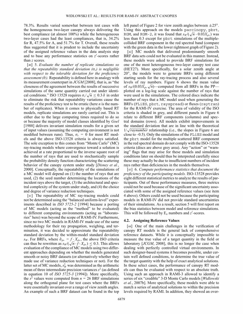
[42] MC models that delivered predominantly smoothBRF data sets could not be evaluated in this manner. Instead,these models were asked to provide BRF simulations forone of the most heterogeneous two-layer canopy test case(HET27). More specifically, for a solar zenith angle at20ı, the models were to generate BRFs using differentstarting seeds for the ray-tracing process and also severallevels of ray numbers. Figure 6 shows the mean valueof sW/(0.03X�*
pn)—computed from all BRFs in the PP—
plotted on a log-log scale against the number of rays thatwere used in the simulations. The colored discs indicate thenumber of rays that a MC model used when generating theBRFs (FLiES, pbrt, rayspread) or fluxes (raytran)for the RAMI-IV exercise. The area of validity of the ISOcriteria is shaded in grey, and different panels in Figure 6relate to different BRF components (columns) and spec-tral domains (rows). All models exhibit improvements inthe standard deviation that are in line with the theoretical1/p
raynumber relationship (i.e., the slopes in Figure 6 areclose to –0.5). Only the simulations of the FLiESmodel andthe pbrt model for the multiple scattered BRF componentin the red spectral domain do not comply with the ISO-13528criteria (discs are above grey area). Any “action” or “warn-ing” flags that may arise for these models and simulationconditions later on should thus be interpreted carefully sincethese may actually be due to insufficient numbers of incidentrays rather than deficiencies in the models themselves.
[43] 6. Compute performance statistics that document theproficiency of the participating models. ISO-13528 provideseight different statistical metrics to analyze the results of par-ticipants. Out of these performance measures, three metricscould not be used because of the significant uncertainty asso-ciated with some of the assigned reference values (see item4 above). Others could not be used because the participatingmodels in RAMI-IV did not provide standard uncertaintiesof their simulations. As a result, section 5 will first report onthe bias statistics between model and reference simulations.This will be followed by En numbers and z0-scores.
4.2. Assigning Reference Values[44] One of the main challenges in the verification of
canopy RT models is the general lack of comprehensivereference datasets. While it is conceptually impossible tomeasure the true value of a target quantity in the field orlaboratory [JCGM, 2008], this is no longer the case whendealing with perfectly controlled virtual environments. Insuch designer-based systems it becomes possible, under cer-tain well defined conditions, to determine the true value ofthe target quantity with the help of exact analytical solutions.In these select cases, the performance of canopy RT mod-els can thus be evaluated with respect to an absolute truth.Using such an approach in RAMI-3 allowed to identify aseries of six “credible” 3-D Monte Carlo models [Widlowskiet al., 2007b]. More specifically, these models were able tomatch a series of analytical solutions to within the precisionlevels required by RAMI. In addition, they showed an over-
6879
WIDLOWSKI ET AL.: RESULTS FOR RAMI-IV ABSTRACT CANOPIES
single−collided BRF single−uncollided BRF multiple−collided BRFR
ED
NIR
total BRF (or albedo)
libratpbrtFLiESrayspread
raytranlibratpbrtFLiESrayspread
libratpbrtFLiESrayspread
libratpbrtFLiESrayspread
raytranlibratpbrtFLiESrayspread
libratpbrtFLiESrayspread
libratpbrtFLiESrayspread
libratpbrtFLiESrayspread
ray numberray number
ray number ray numberray number
ray number
ray number
ray number
Figure 6. Log-log plots of normalized standard deviations (sW/p
n � O�)—derived from BRF (or DHR)simulations of the HET27 test case having a solar zenith angle of 20ı—as a function of the number ofrays that were used by the MC models. The proficiency standard deviation was expressed as 3% of theassigned reference BRF, i.e., O� = 0.03X and n = 10 is the number of BRF replicates (different seedvalues) at a given ray number. The discs indicate the number of rays used by a given model (color) whenperforming RAMI-IV experiments. The grey area indicates compliance with the ISO-13528 criteria. Onlythe raytran data relate to surface albedo (DHR) simulations.
all agreement of �1% across all of their BRF simulationresults. Four of these “credible” RAMI-3 MC models con-tributed to RAMI-IV, namely, DART, librat, raytran,and rayspread. Of these, the DART model had been sub-stantially altered since RAMI-3. DART now makes use of aflux tracking method (rather than MC ray-tracing) such thatit cannot be considered identical to the model analyzed inWidlowski et al. [2007b].
[45] In the context of RAMI-IV, the true values of theradiative quantities are not known a priori. For proficiencytesting, one thus has to make use of section 5.5 (con-sensus value from expert laboratories) and/or section 5.6(consensus value from participants) of ISO-13528 to assignreference values. As indicated previously, the expert modelsthat will be used in RAMI-IV are the “credible” MC mod-els librat and rayspread for BRF simulations and theraytran MC model for the flux simulations. The follow-ing sections will describe in more detail how the assignedreference values (denoted X) were derived from the availablemodel simulations (denoted � for BRFs).4.2.1. Single-Collided and Uncollided BRFs
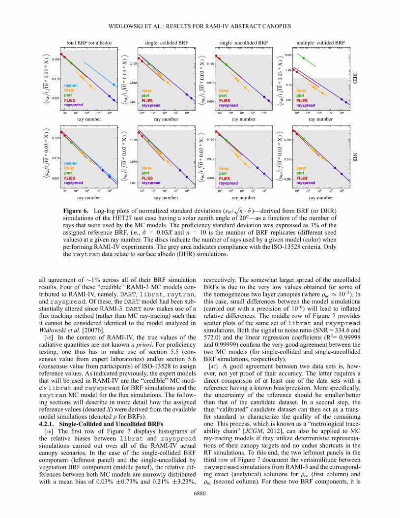
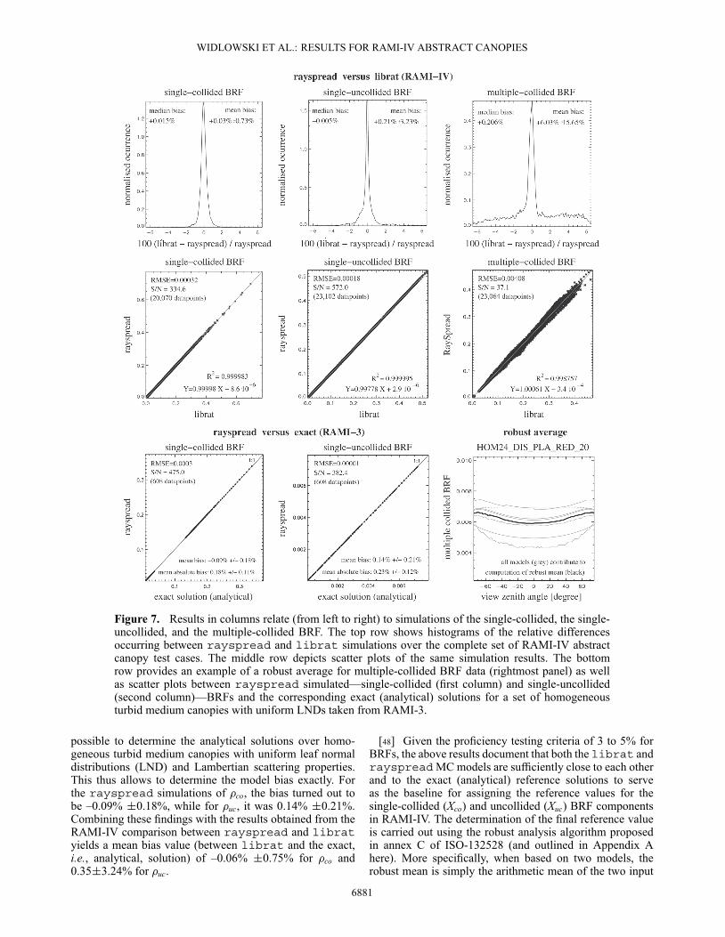
[46] The first row of Figure 7 displays histograms ofthe relative biases between librat and rayspreadsimulations carried out over all of the RAMI-IV actualcanopy scenarios. In the case of the single-collided BRFcomponent (leftmost panel) and the single-uncollided byvegetation BRF component (middle panel), the relative dif-ferences between both MC models are narrowly distributedwith a mean bias of 0.03% ˙0.73% and 0.21% ˙3.23%,
respectively. The somewhat larger spread of the uncollidedBRFs is due to the very low values obtained for some ofthe homogeneous two layer canopies (where �uc � 10–5). Inthis case, small differences between the model simulations(carried out with a precision of 10–6) will lead to inflatedrelative differences. The middle row of Figure 7 providesscatter plots of the same set of librat and rayspreadsimulations. Both the signal to noise ratio (SNR = 334.6 and572.0) and the linear regression coefficients (R2= 0.99998and 0.99999) confirm the very good agreement between thetwo MC models (for single-collided and single-uncollidedBRF simulations, respectively).
[47] A good agreement between two data sets is, how-ever, not yet proof of their accuracy. The latter requires adirect comparison of at least one of the data sets with areference having a known bias/precision. More specifically,the uncertainty of the reference should be smaller/betterthan that of the candidate dataset. In a second step, thethus “calibrated” candidate dataset can then act as a trans-fer standard to characterize the quality of the remainingone. This process, which is known as a “metrological trace-ability chain” [JCGM, 2012], can also be applied to MCray-tracing models if they utilize deterministic representa-tions of their canopy targets and no undue shortcuts in theRT simulations. To this end, the two leftmost panels in thethird row of Figure 7 document the verisimilitude betweenrayspread simulations from RAMI-3 and the correspond-ing exact (analytical) solutions for �co (first column) and�uc (second column). For these two BRF components, it is
6880
WIDLOWSKI ET AL.: RESULTS FOR RAMI-IV ABSTRACT CANOPIES
Figure 7. Results in columns relate (from left to right) to simulations of the single-collided, the single-uncollided, and the multiple-collided BRF. The top row shows histograms of the relative differencesoccurring between rayspread and librat simulations over the complete set of RAMI-IV abstractcanopy test cases. The middle row depicts scatter plots of the same simulation results. The bottomrow provides an example of a robust average for multiple-collided BRF data (rightmost panel) as wellas scatter plots between rayspread simulated—single-collided (first column) and single-uncollided(second column)—BRFs and the corresponding exact (analytical) solutions for a set of homogeneousturbid medium canopies with uniform LNDs taken from RAMI-3.
possible to determine the analytical solutions over homo-geneous turbid medium canopies with uniform leaf normaldistributions (LND) and Lambertian scattering properties.This thus allows to determine the model bias exactly. Forthe rayspread simulations of �co, the bias turned out tobe –0.09% ˙0.18%, while for �uc, it was 0.14% ˙0.21%.Combining these findings with the results obtained from theRAMI-IV comparison between rayspread and libratyields a mean bias value (between librat and the exact,i.e., analytical, solution) of –0.06% ˙0.75% for �co and0.35˙3.24% for �uc.
[48] Given the proficiency testing criteria of 3 to 5% forBRFs, the above results document that both the librat andrayspread MC models are sufficiently close to each otherand to the exact (analytical) reference solutions to serveas the baseline for assigning the reference values for thesingle-collided (Xco) and uncollided (Xuc) BRF componentsin RAMI-IV. The determination of the final reference valueis carried out using the robust analysis algorithm proposedin annex C of ISO-132528 (and outlined in Appendix Ahere). More specifically, when based on two models, therobust mean is simply the arithmetic mean of the two input
6881
WIDLOWSKI ET AL.: RESULTS FOR RAMI-IV ABSTRACT CANOPIES
data. However, because the �co simulations of librat forhomogeneous canopies with anisotropic backgrounds in thered spectral band were resubmitted with a relatively largenoise level, it was decided to base the reference solution forthese cases on the simulation results of the rayspreadmodel only.4.2.2. Multiple Scattered BRFs
[49] The rightmost panels in the first row of Figure 7displays a histogram of relative differences in the multiple-collided BRF simulations of librat and rayspread forthe abstract canopy test cases of RAMI-IV. The mean biasbetween the two MC models is 6.03% ˙ 15.65% (using23,064 data points) with some values in the red spectral band(where �mlt is often rather low) reaching 50% bias or more.The larger spread in the �mlt simulations (compared to the�uc and �co BRF components) is also visible from the scat-terplot in the rightmost panel of the middle row of Figure 7.Here the SNR=37.1 which is only about a tenth of what itwas for �co and �uc. The reasons for these differences are notabsolutely clear at this stage although a preliminary analy-sis points toward an erroneous post-processing of some thelibrat �mlt simulations. While the observed mean ampli-tude of the librat simulated BRF signal appears to besimilar to that of other RT models in RAMI-IV, the angu-lar shape of its �mlt component is often different in particularalong the principal plane.
[50] Due to the lack of exact analytical solutions for�mlt and since the typical bias between the librat andrayspread models exceeded the prescribed criterion forthe proficiency test (i.e., O��mlt = 0.03Xmlt or 0.05Xmlt), it wasdecided to adopt the approach of section 5.6 in ISO-13528(consensus values from participants) to assign reference val-ues for the multiple-collided BRF component (Xmlt). Datasets were excluded from the robust analysis—described inAppendix A—if their noise level (or angular pattern) per-turbed the smoothness of the robust mean along the principalor orthogonal planes. This concerned the �mlt simulationsof (1) pbrt in the red spectral band (all cases) as well asfor the constant slope test cases and for the homogeneoustest cases in the NIR, (2) parcinopy for the homogeneoustwo-layer canopies having a planophile LND below an erec-tophile foliage layer, and (3) RGM-2 for the homogeneoustwo layer test cases HOM27 and HOM28 in the red spectralband for �0 = 50ı. Despite these exceptions, the number ofRT model simulations that were used to compute the robustaverage stayed between 4 and 7. An example of the outcomeof such a robust analysis is shown in the rightmost panel inthe bottom row of Figure 7.4.2.3. Total BRFs
[51] The robust analysis was not applied to the total BRFsimulations that were provided by the RAMI-IV partici-pants. Instead, it was decided to define the assigned refer-ence value for total BRFs (Xtot) as the sum of the assignedreference values of the three BRF components, i.e., Xtot =Xuc + Xco + Xmlt. Similarly, the variance of Xtot was computedas the sum of the variances of the relevant reference values:u2
Xtot= u2
Xuc+ u2
Xco+ u2
Xmlt. This approach ensures consistency.
[52] It should be noted here that ISO-13528 prohibits theevaluation of models/laboratories if their data were used inthe generation of the assigned reference values. To avoidsuch correlation issues within RAMI, every participatingmodel had its own reference value computed. This was done
by excluding the model in question from the list of mod-els contributing to the robust mean. The assigned referencevalue (X*) thus becomes model-specific (Xm
* ) in this study.In the case of �co and �uc, for example, this meant that theassigned reference values for rayspread and libratdiffered from that computed for the remainder of models,whereas for �mlt, the assigned reference value was differentfor every model that contributed to the robust analysis. Thedifferences between the assigned reference BRFs were onaverage less than 0.5% for �co, �uc, and �tot but could reachup to 3% for �mlt.
[53] The robust analysis approach proposed by ISO-13528 delivers also an estimate of the standard uncertaintyof the reference (uX) (see equation A5). For cases where thereference had to be based on a single “credible” model—e.g., when using the librat model as reference for �coand �uc simulations of rayspread (and vice versa)—thenthe value of uX had to be derived by other means. Morespecifically, in such cases, the standard uncertainty was esti-mated as uX = sW/
pn using the BRF data contributing to
Figure 6. Here sW was the average of the standard deviationsobtained from n = 10 different sets of BRF simulations foreach viewing condition along the PP over the HET27 hetero-geneous two layer canopy test case. This process was carriedout using the value of sW corresponding to the smallestnumber of incident rays that were used by the librat andrayspread models to perform the RAMI-IV simulations.The resulting standard uncertainty values were ulibrat�uc
=1.39�10–5 (1.71�10–5) and urayspread�uc = 1.71�10–6 (4.01�10–6)in the red (NIR) and ulibrat�co
= 8.63 � 10–6 (7.22 � 10–5) andurayspread�co = 7.61 � 10–7 (1.04 � 10–5) in the red (NIR).4.2.4. Hemispherical Fluxes
[54] The raytran model was the only “credible” MCmodel to deliver hemispherically integrated fluxes in RAMI-IV. During RAMI-3, it had been shown to match analyticalsolutions of both the foliage absorption and canopy albedoto within the numerical precision required by RAMI (10–6).In section 3, raytran was furthermore shown to con-serve energy (for test cases with Lambertian backgrounds).As such, it was considered appropriate to make use of thesimulations of raytran to assign reference values forhemispherically integrated fluxes in RAMI-IV. In this case,the standard uncertainty of the reference was again estimatedas uX = sW/
pn where sW was the standard deviation of
n = 10 flux simulations carried out with different startingseeds and for ray numbers typically used by raytran forits RAMI-IV flux simulations (compare with the albedo dataof raytran in Figure 6). As such, uR = 5.18�10–6 in the redand 1.37 �10–5 in the NIR. At the same time, and in order notto rely solely on the simulations of a single RT model, it wasdecided to generate a second set of reference values basedon a robust analysis of the hemispherical fluxes generated byall of the RAMI-IV participants.
5. Results for “Abstract Canopy” Cases5.1. RT Model Bias
[55] A detailed analysis of the patterns emerging whentotal BRF differences, i.e., �tot – Xtot, were plotted as a func-tion of the reference value (not shown) allowed to draw thefollowing conclusions:
6882
WIDLOWSKI ET AL.: RESULTS FOR RAMI-IV ABSTRACT CANOPIES
[56] 1. The bias of the models librat, rayspread,and pbrt can be considered independent of the referencevalue in both the red and also the NIR spectral domain. Somelarger deviations were noted for �pbrttot over heterogeneoustest cases with a constant inclination of crowns. These devi-ations are likely to be due to operator glitches since the biaswas directionally selective (as can be seen from the secondpanel of the bottom row in Figure 2).
[57] 2. The bias of the models DART, discret, FDM,FLiES, and parcinopy are likely to be independent ofthe reference value in at least one (typically the red) spectraldomain. Only the range of the biases of �FLiEStot in the NIRseemed to increase consistently with the reference BRF.
[58] 3. The bias of the models inform, RGM, and RGM-2is often rather large and does not exhibit any clear patternwith respect to the assigned reference values. Typically, thebias is smaller in the red band and also evenly distributedaround the zero line in that spectral regime. At the sametime, all three models have a tendency to systematicallyunderestimate the reference value in the NIR. This spectralpattern is likely to be caused by an underestimation of �mlt inthe NIR.
[59] It should be noted that this qualitative analysis ofbias patterns does not account for uncertainties associatedwith the model simulations and/or reference values. Neitherdoes it relate the observed biases to the prescribed standarddeviation of the proficiency test. The following sections willdeal with these aspects in order to determine whether theobserved differences between model and reference valuesare actually relevant.
5.2. En Numbers[60] The En performance statistics is suggested in section
7.5 of ISO-13528 to evaluate the reliability of the expandeduncertainty that individual laboratories claim to have. In thecontext of RAMI, it is defined as
En(m;�, �,�v,�i) =xm
* (�, �,�v,�i) – X*(�, �,�v,�i)qU2
xm*
(�, �,�v,�i) + U2X*
(�, �,�v,�i)(2)
where xm* is the radiative quantity of interest (e.g., a total
BRF, a flux quantity, or one of their components) simulatedby model m for a given spectral (�), structural (�), view-ing (�v), and illumination (�i) related condition. X* is theassigned reference value under these conditions (which ismodel-specific here, i.e., Xm
* ), while the expanded uncer-tainty of the reference UX*
= k � uX*with k = 2 as coverage
factor. The standard uncertainty of the reference uX*was
defined either as in equation (A5) or, for cases where theassigned reference value originates from a single model, asspecified in sections 4.2.3 and 4.2.4. A value of |En| < 1provides objective evidence that the estimates of expandeduncertainty agree with the observed differences between xm
*and X*. Alternatively, one can say that if |En| is less thanunity, then the expanded uncertainties of both the modeland reference data are sufficient to explain the differencesobserved between them. Two different usages of En statisticswill now be presented.5.2.1. Maximum Tolerable Model Uncertainties
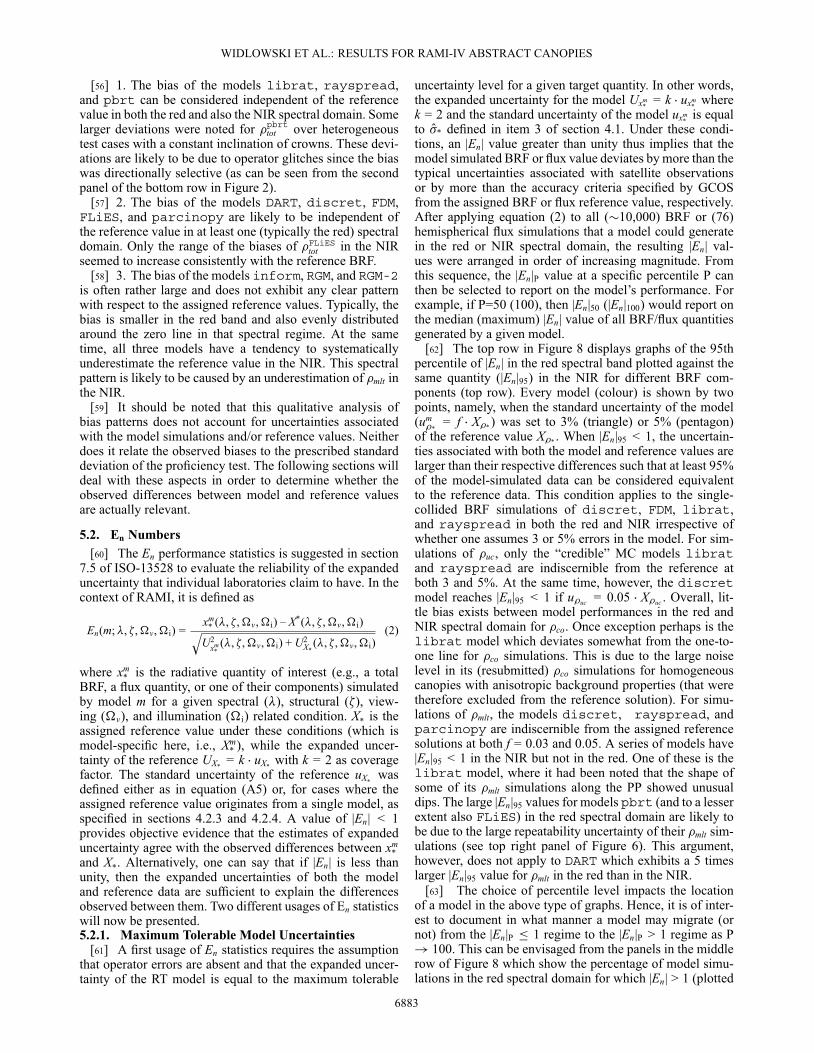
[61] A first usage of En statistics requires the assumptionthat operator errors are absent and that the expanded uncer-tainty of the RT model is equal to the maximum tolerable
uncertainty level for a given target quantity. In other words,the expanded uncertainty for the model Uxm
*= k � uxm
*where
k = 2 and the standard uncertainty of the model uxm*
is equalto O�* defined in item 3 of section 4.1. Under these condi-tions, an |En| value greater than unity thus implies that themodel simulated BRF or flux value deviates by more than thetypical uncertainties associated with satellite observationsor by more than the accuracy criteria specified by GCOSfrom the assigned BRF or flux reference value, respectively.After applying equation (2) to all (�10,000) BRF or (76)hemispherical flux simulations that a model could generatein the red or NIR spectral domain, the resulting |En| val-ues were arranged in order of increasing magnitude. Fromthis sequence, the |En|P value at a specific percentile P canthen be selected to report on the model’s performance. Forexample, if P=50 (100), then |En|50 (|En|100) would report onthe median (maximum) |En| value of all BRF/flux quantitiesgenerated by a given model.
[62] The top row in Figure 8 displays graphs of the 95thpercentile of |En| in the red spectral band plotted against thesame quantity (|En|95) in the NIR for different BRF com-ponents (top row). Every model (colour) is shown by twopoints, namely, when the standard uncertainty of the model(um�*
= f � X�* ) was set to 3% (triangle) or 5% (pentagon)of the reference value X�* . When |En|95 < 1, the uncertain-ties associated with both the model and reference values arelarger than their respective differences such that at least 95%of the model-simulated data can be considered equivalentto the reference data. This condition applies to the single-collided BRF simulations of discret, FDM, librat,and rayspread in both the red and NIR irrespective ofwhether one assumes 3 or 5% errors in the model. For sim-ulations of �uc, only the “credible” MC models libratand rayspread are indiscernible from the reference atboth 3 and 5%. At the same time, however, the discretmodel reaches |En|95 < 1 if u�uc = 0.05 � X�uc . Overall, lit-tle bias exists between model performances in the red andNIR spectral domain for �co. Once exception perhaps is thelibrat model which deviates somewhat from the one-to-one line for �co simulations. This is due to the large noiselevel in its (resubmitted) �co simulations for homogeneouscanopies with anisotropic background properties (that weretherefore excluded from the reference solution). For simu-lations of �mlt, the models discret, rayspread, andparcinopy are indiscernible from the assigned referencesolutions at both f = 0.03 and 0.05. A series of models have|En|95 < 1 in the NIR but not in the red. One of these is thelibrat model, where it had been noted that the shape ofsome of its �mlt simulations along the PP showed unusualdips. The large |En|95 values for models pbrt (and to a lesserextent also FLiES) in the red spectral domain are likely tobe due to the large repeatability uncertainty of their �mlt sim-ulations (see top right panel of Figure 6). This argument,however, does not apply to DART which exhibits a 5 timeslarger |En|95 value for �mlt in the red than in the NIR.
[63] The choice of percentile level impacts the locationof a model in the above type of graphs. Hence, it is of inter-est to document in what manner a model may migrate (ornot) from the |En|P � 1 regime to the |En|P > 1 regime as P! 100. This can be envisaged from the panels in the middlerow of Figure 8 which show the percentage of model simu-lations in the red spectral domain for which |En| > 1 (plotted
6883
WIDLOWSKI ET AL.: RESULTS FOR RAMI-IV ABSTRACT CANOPIES
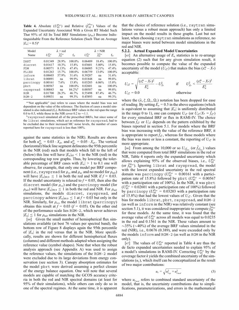
Table 4. Absolute (U�tot95 ) and Relative (Qf �tot
95 ) Values of theExpanded Uncertainty Associated With a Given RT Model SuchThat 95% of All Its Total BRF Simulations (�tot) Become Indis-tinguishable From the Reference Solution (Such That on Average|En| = 0.5)a
Model � = red � = NIRName U�tot
95 Qf �tot95 fN U�tot
95 Qf �tot95 fN
DART 0.01349 28.9% 100.0% 0.06489 18.4% 100.0%discret 0.01617 10.3% 15.8% 0.03601 5.80% 15.8%FDM 0.00571 8.13% 47.4% 0.06005 9.21% 47.4%FLiES 0.01263 15.7% 100.0% 0.06759 13.0% 100.0%inform 0.08603 57.9% 31.6% 0.39287 na 31.6%librat 0.00091 na 99.9% 0.01848 na 99.8%parcinopy 0.00161 7.6% 15.8% 0.03203 6.06% 15.8%pbrt 0.00567 na 100.0% 0.02601 na 100.0%rayspread 0.00043 na 84.2%b 0.00507 na 99.8%RGM 0.01700 26.3% 46.7% 0.55498 87.4% 46.7%RGM-2 0.09831 na 99.3% 0.45893 na 99.3%
a“Not applicable” (na) refers to cases where the model bias was notdependent on the value of the reference. The fraction of cases a model sim-ulated is also indicated (fN). Reference BRF values in the red span the range0.0 to 0.5, while those in the NIR cover 0.2 to �1.1.
brayspread simulated all of the prescribed BRFs, but since some ofthe librat simulations, which act as reference for rayspread, had tobe excluded due to their increased MC noise levels, the number of casesreported here for rayspread is less than 100%.
against the same statistics in the NIR). Results are shownfor both um
�*= 0.03 � X�* and um
�*= 0.05 � X�* . The vertical
(horizontal) black line segment delineates the 95th percentilein the NIR (red) such that models which fall to the left of(below) this line will have |En|95 < 1 in the NIR (red) in thecorresponding top row graphs. Thus, by lowering the toler-able percentage of BRF cases with |En| > 1 to 0.1 one willobserve, for example, that only one model per BRF compo-nent (i.e., rayspread for �co and �uc and no model for �mlt)will have |En|99.9 � 1 in both the red and NIR if f = 0.03.If the model uncertainty is relaxed to f = 0.05, then also thediscret model (for �co) and the parcinopy model (for�mlt) will have |En|99.9 � 1 in both the red and NIR. For �mltsimulations, the models discret, rayspread, andparcinopy achieve |En|99.9 � 1 at f = 0.03 but only in theNIR. Similarly, for �co, the model librat (parcinopy)obtains this result at f = 0.03 (f = 0.05). On the other endof the performance scale lies RGM-2, which never achieves|En| � 1 for �mlt simulations in the NIR.
[64] Given the small number of hemispherical flux sim-ulations available (at best 76 values per spectral band), thebottom row of Figure 8 displays again the 95th percentileof |En| in the red versus that in the NIR. More specifi-cally, results are shown for different hemispherical fluxes(columns) and different methods adapted when assigning thereference value (symbol shapes). Note that when the robustanalysis approach (see Appendix A) was used to assignthe reference values, the simulations of the RGM-2 modelwere excluded due to its large deviations from energy con-servation (see section 3). Canopy absorption estimates forthe model pbrt were derived assuming a perfect closureof the energy balance equation. One will note that severalmodels are capable of matching the GCOS accuracy crite-ria in both the red and NIR spectral domains (at least for95% of their simulations), while others can only do so inone of the spectral regimes. At the same time, it is apparent
that the choice of reference solution (i.e., raytran simu-lations versus a robust mean approach) has only a limitedimpact on the model results in these graphs. Last but notleast, when choosing raytran simulations as reference, nomajor biases were noted between model simulations in thered and NIR.5.2.2. Actual Expanded Model Uncertainties
[65] An alternative usage of En statistics is to re-arrangeequation (2) such that for any given simulation result, itbecomes possible to compute the value of the expandeduncertainty of the model (Uxm
*) that makes the bias (xm
* – X*)acceptable:
Uxm*
=
s(xm
* – X*)2
E2n
– U2X*
if U2X*
<(xm
* – X*)2
E2n
Uxm*
= 0.0 otherwise
where the (�, �,�v,�i) notation has been dropped for easeof reading. By setting En = 0.5 in the above equations (whichis equivalent to assuming that |En| is uniformly distributedin the range 0 to 1), one can compute Uxm
*(or Uxm
*/X* = Qfxm
*)
for every simulated BRF or flux in RAMI-IV. The choicebetween Qfxm
*or Uxm
*depends on the pattern exhibited by the
biases reported in section 5.1. For models where the BRFbias was increasing with the value of the reference BRF, itis appropriate to report Qfxm
*, whereas for those models where
the bias was more or less a constant, the reporting of Uxm*
ismore appropriate.
[66] From among the 10,000 or so Uxm�tot (or Qfxm
�tot ) valuesthat were computed from total BRF simulations in the red orNIR, Table 4 reports only the expanded uncertainty whichallows explaining 95% of the observed biases, i.e., U�tot
95(or Qf �tot
95 ). Ignoring librat and rayspread, the modelwith the lowest expanded uncertainty in the red spectraldomain was parcinopy (U�tot
95 = 0.00161 with a partici-pation rate of 15.8%) followed by pbrt (U�tot
95 = 0.00567with a participation rate of 100%). In the NIR, it was pbrt(U�tot
95 = 0.02601 with a participation rate of 100%) followedby parcinopy (U�tot
95 = 0.03203 with a participation rateof 15.8%) that had the lowest values of Uxm
*. Given that the
bias for models librat, pbrt, rayspread, and RGM-2(as well as inform in the NIR) was relatively constant (seesection 5.1), it was considered inappropriate to compute Qf �tot
95for these models. At the same time, it was found that theaverage value of U�tot
95 across all models was equal to 0.0235in the red and 0.1561 in the NIR. These values amount to�35% (�40%) of the average BRF values simulated in thered (NIR), i.e., 0.0676 (0.389), and were exceeded only bythe models inform and RGM-2 (as well as RGM in the NIRonly).
[67] The values of U�tot95 reported in Table 4 are thus the
de facto expanded uncertainties needed to explain 95% ofa model’s simulations in RAMI-IV. Correcting U�tot
95 by thecoverage factor k yields the combined uncertainty of the sim-ulations (uc), which itself can be conceptualized as the resultof two major contributions:
uc =q
u2cop
+ u2cmod
(3)
where ucmod refers to combined standard uncertainty of themodel, that is, the uncertainty contributions due to simpli-fications, parameterizations, and errors in the mathematical
6884
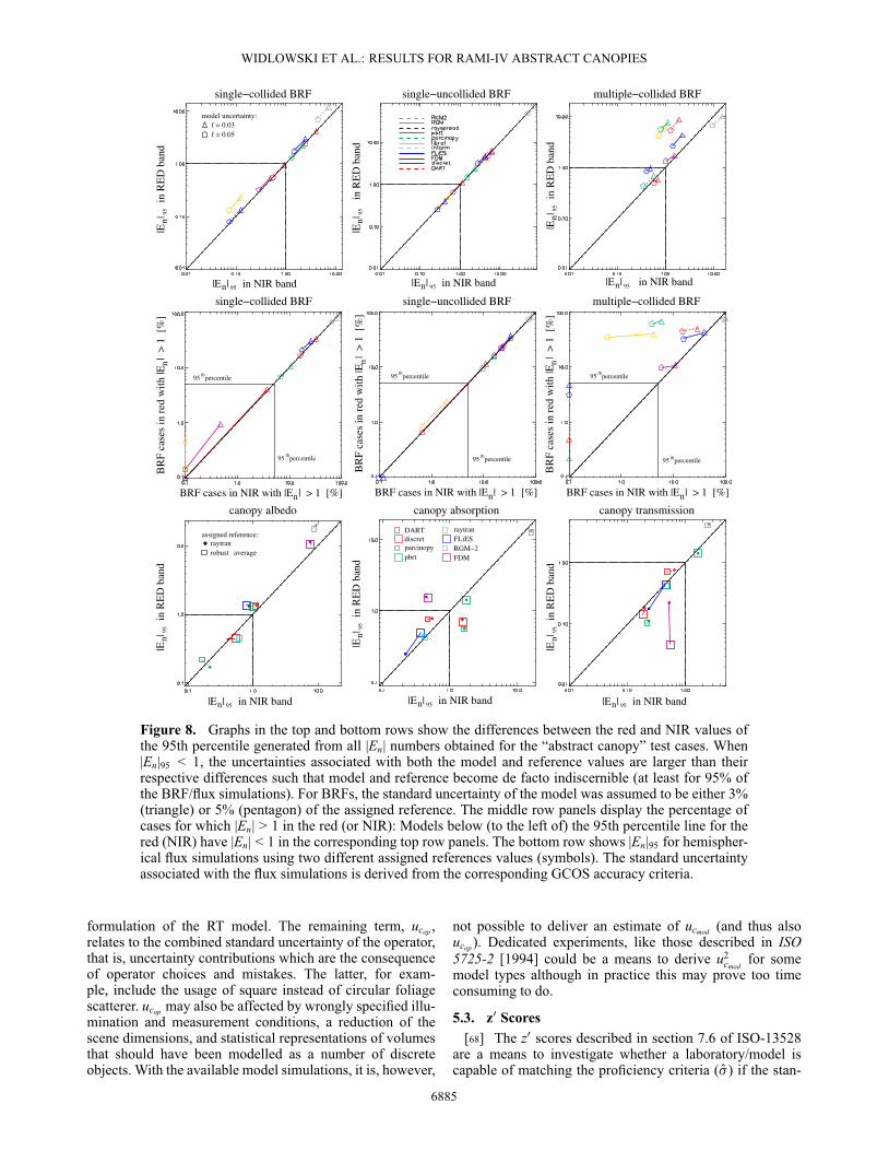
WIDLOWSKI ET AL.: RESULTS FOR RAMI-IV ABSTRACT CANOPIES
Figure 8. Graphs in the top and bottom rows show the differences between the red and NIR values ofthe 95th percentile generated from all |En| numbers obtained for the “abstract canopy” test cases. When|En|95 < 1, the uncertainties associated with both the model and reference values are larger than theirrespective differences such that model and reference become de facto indiscernible (at least for 95% ofthe BRF/flux simulations). For BRFs, the standard uncertainty of the model was assumed to be either 3%(triangle) or 5% (pentagon) of the assigned reference. The middle row panels display the percentage ofcases for which |En| > 1 in the red (or NIR): Models below (to the left of) the 95th percentile line for thered (NIR) have |En| < 1 in the corresponding top row panels. The bottom row shows |En|95 for hemispher-ical flux simulations using two different assigned references values (symbols). The standard uncertaintyassociated with the flux simulations is derived from the corresponding GCOS accuracy criteria.
formulation of the RT model. The remaining term, ucop ,relates to the combined standard uncertainty of the operator,that is, uncertainty contributions which are the consequenceof operator choices and mistakes. The latter, for exam-ple, include the usage of square instead of circular foliagescatterer. ucop may also be affected by wrongly specified illu-mination and measurement conditions, a reduction of thescene dimensions, and statistical representations of volumesthat should have been modelled as a number of discreteobjects. With the available model simulations, it is, however,
not possible to deliver an estimate of ucmod (and thus alsoucop ). Dedicated experiments, like those described in ISO5725-2 [1994] could be a means to derive u2
cmodfor some
model types although in practice this may prove too timeconsuming to do.
5.3. z0 Scores[68] The z0 scores described in section 7.6 of ISO-13528
are a means to investigate whether a laboratory/model iscapable of matching the proficiency criteria ( O�) if the stan-
6885
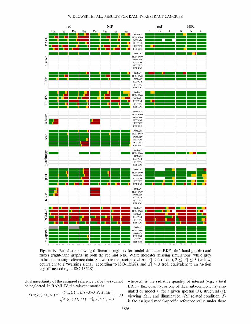
WIDLOWSKI ET AL.: RESULTS FOR RAMI-IV ABSTRACT CANOPIES
Figure 9. Bar charts showing different z0 regimes for model simulated BRFs (left-hand graphs) andfluxes (right-hand graphs) in both the red and NIR. White indicates missing simulations, while greyindicates missing reference data. Shown are the fractions where |z0| < 2 (green), 2 � |z0| � 3 (yellow,equivalent to a “warning signal” according to ISO-13528), and |z0| > 3 (red, equivalent to an “actionsignal” according to ISO-13528).
dard uncertainty of the assigned reference value (uX) cannotbe neglected. In RAMI-IV, the relevant metric is
z0(m;�, �,�v,�i) =xm
* (�, �,�v,�i) – X*(�, �,�v,�i)qO�2(�, �,�v,�i) + u2
X*(�, �,�v,�i)
(4)
where xm* is the radiative quantity of interest (e.g., a total
BRF, a flux quantity, or one of their sub-components) sim-ulated by model m for a given spectral (�), structural (�),viewing (�v), and illumination (�i) related condition. X*is the assigned model-specific reference value under these
6886
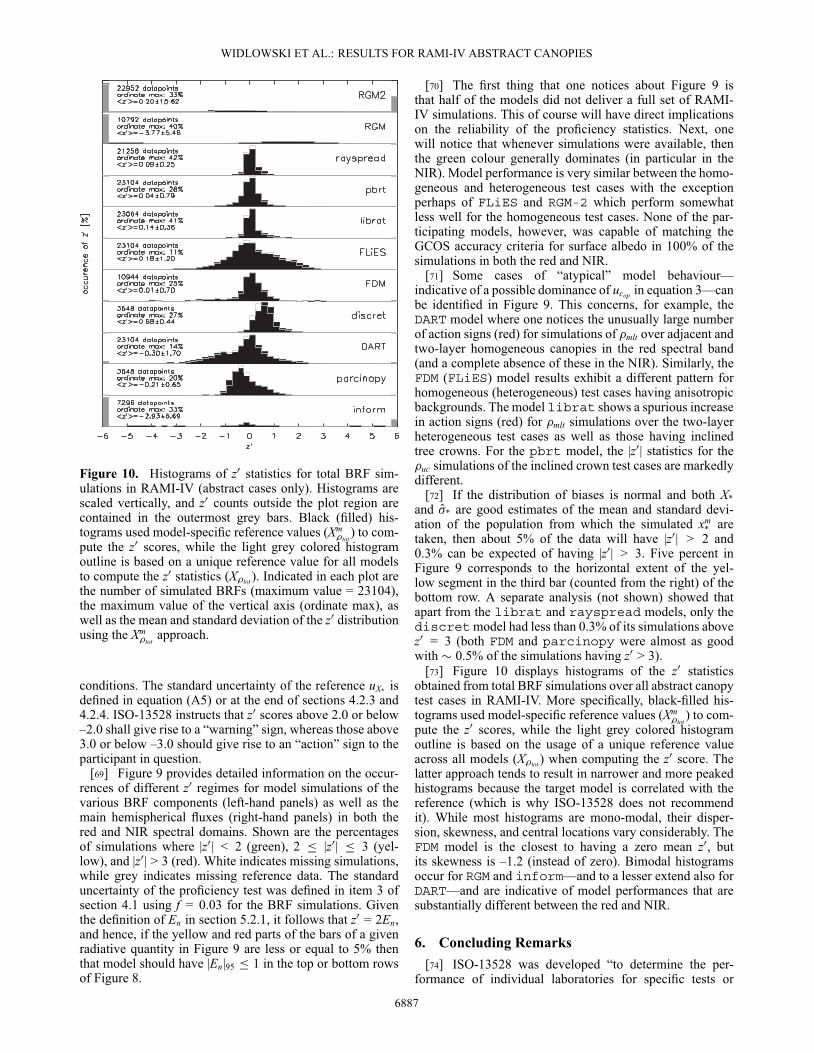
WIDLOWSKI ET AL.: RESULTS FOR RAMI-IV ABSTRACT CANOPIES
Figure 10. Histograms of z0 statistics for total BRF sim-ulations in RAMI-IV (abstract cases only). Histograms arescaled vertically, and z0 counts outside the plot region arecontained in the outermost grey bars. Black (filled) his-tograms used model-specific reference values (Xm
�tot) to com-
pute the z0 scores, while the light grey colored histogramoutline is based on a unique reference value for all modelsto compute the z0 statistics (X�tot ). Indicated in each plot arethe number of simulated BRFs (maximum value = 23104),the maximum value of the vertical axis (ordinate max), aswell as the mean and standard deviation of the z0 distributionusing the Xm
�totapproach.
conditions. The standard uncertainty of the reference uX* isdefined in equation (A5) or at the end of sections 4.2.3 and4.2.4. ISO-13528 instructs that z0 scores above 2.0 or below–2.0 shall give rise to a “warning” sign, whereas those above3.0 or below –3.0 should give rise to an “action” sign to theparticipant in question.
[69] Figure 9 provides detailed information on the occur-rences of different z0 regimes for model simulations of thevarious BRF components (left-hand panels) as well as themain hemispherical fluxes (right-hand panels) in both thered and NIR spectral domains. Shown are the percentagesof simulations where |z0| < 2 (green), 2 � |z0| � 3 (yel-low), and |z0| > 3 (red). White indicates missing simulations,while grey indicates missing reference data. The standarduncertainty of the proficiency test was defined in item 3 ofsection 4.1 using f = 0.03 for the BRF simulations. Giventhe definition of En in section 5.2.1, it follows that z0 = 2En,and hence, if the yellow and red parts of the bars of a givenradiative quantity in Figure 9 are less or equal to 5% thenthat model should have |En|95 � 1 in the top or bottom rowsof Figure 8.
[70] The first thing that one notices about Figure 9 isthat half of the models did not deliver a full set of RAMI-IV simulations. This of course will have direct implicationson the reliability of the proficiency statistics. Next, onewill notice that whenever simulations were available, thenthe green colour generally dominates (in particular in theNIR). Model performance is very similar between the homo-geneous and heterogeneous test cases with the exceptionperhaps of FLiES and RGM-2 which perform somewhatless well for the homogeneous test cases. None of the par-ticipating models, however, was capable of matching theGCOS accuracy criteria for surface albedo in 100% of thesimulations in both the red and NIR.
[71] Some cases of “atypical” model behaviour—indicative of a possible dominance of ucop in equation 3—canbe identified in Figure 9. This concerns, for example, theDART model where one notices the unusually large numberof action signs (red) for simulations of �mlt over adjacent andtwo-layer homogeneous canopies in the red spectral band(and a complete absence of these in the NIR). Similarly, theFDM (FLiES) model results exhibit a different pattern forhomogeneous (heterogeneous) test cases having anisotropicbackgrounds. The model librat shows a spurious increasein action signs (red) for �mlt simulations over the two-layerheterogeneous test cases as well as those having inclinedtree crowns. For the pbrt model, the |z0| statistics for the�uc simulations of the inclined crown test cases are markedlydifferent.
[72] If the distribution of biases is normal and both X*and O�* are good estimates of the mean and standard devi-ation of the population from which the simulated xm
* aretaken, then about 5% of the data will have |z0| > 2 and0.3% can be expected of having |z0| > 3. Five percent inFigure 9 corresponds to the horizontal extent of the yel-low segment in the third bar (counted from the right) of thebottom row. A separate analysis (not shown) showed thatapart from the librat and rayspread models, only thediscretmodel had less than 0.3% of its simulations abovez0 = 3 (both FDM and parcinopy were almost as goodwith � 0.5% of the simulations having z0 > 3).
[73] Figure 10 displays histograms of the z0 statisticsobtained from total BRF simulations over all abstract canopytest cases in RAMI-IV. More specifically, black-filled his-tograms used model-specific reference values (Xm
�tot) to com-
pute the z0 scores, while the light grey colored histogramoutline is based on the usage of a unique reference valueacross all models (X�tot ) when computing the z0 score. Thelatter approach tends to result in narrower and more peakedhistograms because the target model is correlated with thereference (which is why ISO-13528 does not recommendit). While most histograms are mono-modal, their disper-sion, skewness, and central locations vary considerably. TheFDM model is the closest to having a zero mean z0, butits skewness is –1.2 (instead of zero). Bimodal histogramsoccur for RGM and inform—and to a lesser extend also forDART—and are indicative of model performances that aresubstantially different between the red and NIR.
6. Concluding Remarks[74] ISO-13528 was developed “to determine the per-
formance of individual laboratories for specific tests or
6887
WIDLOWSKI ET AL.: RESULTS FOR RAMI-IV ABSTRACT CANOPIES
measurements.” This contribution made use of the ISO-13528 standard to evaluate physics-based computer simula-tion models that mimic the transfer of radiation in vegetationcanopies. After a series of initial consistency checks, thisprocedure involved (1) the definition of a tolerance criteriasuitable for the determination of proficiency in RT modelsimulations, (2) the definition of a sufficiently precise ref-erence solution against which the candidate models couldbe compared, and (3) the selection of appropriate evaluationmetrics to quantify the performance of the RT models.
[75] The choice of proficiency criteria ( O�) is crucial forthe outcome of intercomparison efforts. For BRF simula-tions, we set O� to 3% and 5% of the reference value inanalogy with vicarious calibration efforts. For hemispheri-cal fluxes, we made use of the GCOS accuracy criteria forsurface albedo and FAPAR to derive O� . Due to missing infor-mation in GCOS [2011], we assumed a (type B) rectangulardistribution of the biases within the maximum tolerable devi-ation ranges proposed by GCOS. This choice obviously hasan impact on the likelihood of models to comply with theproficiency test. Ideally, GCOS should provide all necessaryelements to allow for an unambiguous evaluation of ECVcompliance. As a minimum, the percentiles of the ECV pop-ulation that must comply with the GCOS accuracy criteriashould be provided. For example, one could specify that100%, 99%, or only 95% of the ECV retrievals (within agiven time frame or geographical region) must fall withinthe GCOS recommended accuracy level. Additionally, theshape of the distribution of biases could be specified.
[76] The reliability of the reference solution is anotherimportant item in proficiency testing. For single-scatteredBRF components, it was possible to use the simulations ofthe librat and rayspreadMonte Carlo models becausethey matched the analytical solutions to within a fraction of1%. For the multiple-scattered BRF component, the robustanalysis method that is proposed in Annex C of ISO-13528was used. For hemispherical fluxes, both the simulations ofthe raytran Monte Carlo model and the robust analysisapproach were used. ISO-13528 points out that the stan-dard uncertainty of the reference solution ideally should notexceed 30% of the proficiency criteria ( O�). This require-ment, however, was rarely satisfied when the robust averageapproach was used to assign a reference value. Whereverpossible, efforts should thus focus on identifying and usingcredible reference models instead.
[77] It was found that some of the more deviating mod-els had never participated in previous phases of RAMI.Whether the differences observed in the current model com-parison effort were caused by operator errors/choices orwere genuine to the RT formulation/implementation of thesemodels could not be determined on the basis of the availabledata. However, the fact that all test cases in RAMI-IV werenew and that some “atypical” model behavior was noted inFigure 9, both point to an increased likelihood of operator-induced errors. In fact, RAMI-1 to RAMI-3 showed that therepetition of a given set of experiments in successive inter-comparison rounds lead to a gradual improvement of (most)models. This is so because developers gradually identify andremove model weaknesses and software errors, and improvethe manner in which the RAMI test cases are implementedin the participating models. A more rigorous approach to thismatter would require evaluating the repeatability of Monte
Carlo models as proposed in ISO 5725-2 and comparing theresults with the actual expanded uncertainties as discussedin section 5.2.2.
[78] While the number of measurements that are usedin laboratory intercomparisons is relatively small (typically< 100), the number of total BRF simulations requested forthis proficiency test exceeded 20,000. It is thus not surpris-ing that none of the participating RT models had a 100%success rate (i.e., z0 < 2) for total BRF simulations. The onlyexception to this are the librat and rayspread modelsthat were, however, used to assign the reference solution forthe single-scattered BRF components. Similarly, for surfacealbedo simulations in the red and NIR, not a single partic-ipant was always matching the GCOS accuracy criteria forall six of the prescribed canopy architecture types. If therequired success rate is reduced to 95% or even 90%, thenthe number of compliant models increases of course.
[79] Gaussian distributions of the biases and z0 scoresenable one to verify whether the number of outliers (i.e., thenumber of biases > 3 O� or the number of z0 scores > 2 or3) is actually in line with the theoretical expectation. Apartfrom model and operator biases, the non-Gaussian distribu-tions of z0 may also be due to inadequate sampling of canopyscenarios from the overall population of possible canopyarchitectures. In fact, if one ignores spectral, illumination,and viewing conditions, only 19 different canopy architec-tures remain (10 for the HOM cases and 9 for the HET).Some RT models submitted simulation results for less thana quarter of these. Such limited verification efforts possesslittle weight regarding the overall quality of a given modeland furthermore complicate the interpretation of results fromdifferent models. The latter is because some operators applytheir models only to test cases for which they were designed(e.g., 1-D models were not applied to 3-D test cases), whileothers run their model also on experiments that are likelyto cause larger deviations (e.g., inform was designed foractual canopies but also delivered results for the abstractcanopy cases).
[80] RAMI advocates a universal model verification strat-egy based on sufficiently large sets of test cases and qual-ified references. This is addressed through intercomparisonrounds (RAMI phases) that are carried out at multi-annualintervals (i.e., 1999, 2002, and 2005). Each phase includesthe experiments of the previous round (such as to enableparticipants to update/rectify their scores). Once reliableRAMI reference solutions have been established in thismanner, they are transferred to the RAMI On-line Checker(ROMC) while RAMI continues with a new set of test cases.This approach is in line with ISO-13528 which specificallyencourages continued proficiency testing. It also enablesmodel developers (and users) to autonomously verify thequality of a given modelling tool via the ROMC instead ofhaving to wait for the next phase of RAMI.
[81] Product certification is well suited to increase userconfidence. In particular, in the manufacturing industries,new products can only enter the market after having passeda set of rigorous tests that certify their compliance with pre-defined quality objectives. By analogy, model certificationwould be a highly desirable aspect in efforts to improvethe credibility of studies relying on canopy RT simulations.Conceptually, the development of a model certification plat-form requires access to (1) reliable procedures and criteria to
6888
WIDLOWSKI ET AL.: RESULTS FOR RAMI-IV ABSTRACT CANOPIES
assess and quantify the performance of models and (2) easy-to-use interfaces allowing interested parties to autonomouslyperform model evalutions. The latter can be addressed byweb-based facilities, like the ROMC. The former should beaddressed by international standards, like ISO-13528, thatmake use of agreed-upon methodologies. All elements arethus in hand now to move toward a community-approvedQA/QC system capable of standardised, user-friendly, andapplication-specific certifications of RT model quality.
Appendix A: Robust Analysis[82] The term “robust average” and “robust standard
deviation” should be understood to mean estimates of thepopulation mean or the population standard deviation cal-culated using a robust algorithm [ISO 13528, 2005]. Themethodology presented below has been transcribed from thatpresented in annex C.1 of the ISO13528:2005 standard inorder to match the nomenclature and context of the RAMIexercise.
[83] If N models have generated a BRF value for a givenviewing and illumination configuration, then denote the dif-ferent values of BRFs, when sorted into increasing order,by �1, �2, : : : , �i, : : : , �N. Next denote the robust averageand robust standard deviation of these data by �* and s*
�.Calculate initial values for �* and s*
� as
�* = median of �i (i = 1, 2, : : : , N) (A1)s*� = 1.483 � median of |�i – �*| (i = 1, 2, : : : , N) (A2)
[84] Update the values of �* and s*� as follows. First,
compute ı = 1.5 � s*�. Then, for each �i (i = 1, 2, : : : , N),
calculate
�*i =
8̂<̂:�* – ı if �i < �* – ı�* + ı if �i > �* + ı�i otherwise
[85] Next, compute the new values of �* and s*� from
�* =1N
NXi
�*i (A3)
s*� = 1.134 �
vuut 1N – 1
NXi
��*
i – �*�2 (A4)
[86] The robust estimates of �* and s*� may then be
derived by an iterative process, that is, by updating the val-ues of �* and s*
� using the modified data until the processfinally converges. Convergence was assumed to exist when�* was stable within the precision requirements imposed byRAMI, i.e., to within 10–6.
[87] Finally, the standard uncertainty uX of the robustmean can be estimated as
uX = 1.25 � s*�/p
N (A5)
where according to ISO 13528 [2005], the “factor 1.25 rep-resents the ratio of the standard deviation of the medianto the standard deviation of the arithmetic mean, for largesamples (N > 10) from a normal distribution. For nor-mally distributed data, the standard deviation of a robust
average calculated using the algorithm in this appendix isnot known, but will fall somewhere between the standarddeviation of the arithmetic mean and the standard deviationof the median, so the above formula gives a conservativeestimate of the standard uncertainty.”
[88] Acknowledgments. RAMI would not have been possible with-out the support of Alan Belward, head of the Land Resource Managementunit, and Frank Raes, head of the Climate Risk Monitoring unit, both atthe Institute for Environment and Sustainability of the European Commis-sion’s Joint Research Centre in Ispra, Italy. The constructive comments oftwo anonymous reviewers and Jouni Peltoniemi on earlier drafts of thismanuscript are gratefully acknowledged. The technical assistance of Mon-ica Robustelli and the helpful advice of and discussions with the membersof the RAMI Advisory Body is also thankfully acknowledged here.
ReferencesAtzberger, C. (2000), Development of an invertible forest reflectance
model: The infor-model, in A Decade of Trans-European Remote Sens-ing Cooperation. Proceedings of the 20th EARSeL Symposium Dresden,Germany, 14–16 June 2000, edited by M. Buchroithner, pp. 39–44, CRCPress/Balkema, Leiden, The Netherlands.
Bruegge, C. J., N. L. Chrien, R. R. Ando, D. J. Diner, W. A. Abdou, M. C.Helmlinger, S. H. Pilorz, and K. J. Thome (2002), Early validation of themulti-angle imaging spectroradiometer (MISR) radiometric scale, IEEETrans. Geosci. Remote Sens., 40, 1477–1492.
Chelle, M. (1997), Développement d’un modèle de radiosité mixtepour simuler la distribution du rayonnement dans les couverts vege-taux, PhD Thesis, Université de Rennes I. ftp://ftp.irisa.fr/techreports/theses/1997/chelle.ps.gz.
Chelle, M. (2006), Could plant leaves be treated as Lambertian surfacesin dense crop canopies to estimate light absorption? Ecol. Modell., 198,219–228.
Chen, J. M., and J. Cihlar (1995), Plant canopy gap size analysis theoryfor improving optical measurements of leaf area index, Appl. Opt., 34,6211–6222.
Disney, M. I., P. Lewis, and P. R. J. North (2000), Monte Carlo raytracingin optical canopy reflectance modelling, Remote Sens. Rev., 18, 163–196.
Disney, M. I., P. Lewis, M. Bouvet, A. Prieto-Blanco, and S. Hancock(2009), Quantifying surface reflectivity for spaceborne lidar via two inde-pendent methods, IEEE Trans. Geosci. Remote Sens., 47(10), 3262–3271,doi:10.1109/TGRS.2009.2019268.
Gastellu-Etchegorry, J.-P., V. Demarez, V. Pinel, and F. Zagolski (1996),Modeling radiative transfer in heterogeneous 3-D vegetation canopies,Remote Sens. Environ., 58, 131–156.
Gastellu-Etchegorry, J.-P., E. Martin, and F. Gascon (2004), Dart: A 3Dmodel for simulating satellite images and studying surface radiationbudget, Int. J. Remote Sens., 25, 73–96.
GCOS (2011), Systematic observon requirements for satellite-based dataproducts for climate (2011 update), supplemental details to the satellite-based component of the ’implementation plan for the global observingsystem for climate in support of the UNFCCC (2011 update)’. GCOS-154, Global Climate Observing System (GCOS), World MeteorogicalOrganisation.
Gerboles, M., et al. (2011), Interlaboratory comparison exercise for thedetermination of As, Cd, Ni and PM10 in Europe, Atmos. Environ., 45,3488–3499.
Gobron, N., B. Pinty, M. M. Verstraete, and Y. Govaerts (1997), A semi-discrete model for the scattering of light by vegetation, J. Geophys. Res.,102, 9431–9446.
Goel, N. (1988), Models of vegetation canopy reflectance and their use inestimation of biophysical parameters from reflectance data, Remote Sens.Rev., 4, 1–212.
Goel, N. S., and D. E. Strebel (1984), Simple beta distribution rep-resentation of leaf orientation in vegetation canopies, Agron. J., 76,800–803.
Govaerts, Y. (1995), A model of light scattering in three-dimensional plantcanopies: A Monte Carlo ray tracing approach, Ph. D. thesis, UniversitéCatholique de Louvain-la-Neuve, Département de Physique, 2, Chemindu Cyclotron, B–1348 Louvain-la-Neuve, Belgique.
Huang, H., M. Chen, and Q. Liu (2009), A realistic structure model forlarge-scale surface leaving radiance simulation of forest canopy andaccuracy assessment, Int. J. Remote Sens., 30(20), 5421–5439.
Hund, E., D. L. Massart, and J. Smeyers-Verbeke (2000), Inter-laboratorystudies in analytical chemistry, Anal. Chim. Acta, 423, 145–165.
ISO 13528 (2005), Statistical methods for use in proficiency test-ing by interlaboratory comparisons, International Standard, ISO
6889
WIDLOWSKI ET AL.: RESULTS FOR RAMI-IV ABSTRACT CANOPIES
13528:2005(E), 66 pp., International Organization for Standardization,ISO/TC6-SC6, Geneva, Switzerland.
ISO 5725-2 (1994), Accuracy (trueness and precision) of measurementmethods and results—Part 2:, International Standard, ISO 5725-2:1994(E), 42 pp., International Organization for Standardization, ISO/TC69-SC6, Geneva, Switzerland.
ISO 5725-3 (1994), Accuracy (trueness and precision) of measurementmethods and results—Part 3:, International Standard, ISO 5725-3:1994(E), 25 pp., International Organization for Standardization, ISO/TC69-SC6, Geneva, Switzerland.
JCGM (2008), Evaluation of measurement data—Guide to the expressionof uncertainty in measurement, GUM 1995 with minor corrections JCGM100:2008. Joint Committee for Guides in Metrology (JCGM), Bureauinternational des poids et mesures (BIPM) and other members of JCGM.
JCGM (2012), International vocabulary of metrology—Basic and generalconcepts and associated terms (VIM), 3rd edition, VIM 2008 with minorcorrections JCGM 200:2012. Joint Committee for Guides in Metrology(JCGM), Bureau international des poids et mesures (BIPM) and othermembers of JCGM.
Kallel, A. (2010), Vegetation radiative transfer modeling based on vir-tual flux decomposition, J. Quant. Spectrosc. Radiat. Transfer, 111,1389–1405.
Kallel, A. (2012), Extension of virtual flux decomposition model to the caseof two vegetation layers: FDM-2, J. Quant. Spectrosc. Radiat. Transfer,113, 440–460.
Kneubühler, M., M. Schaepman, K. Thome, F. Baret, and A. Müller (2002),Calibration and validation of Envisat MERIS. Part 1: Vicarious cali-bration at Rail Road valley Playa (NV), Proceedings of MERIS level 2validation Workshop, ESRIN, Frascati, Italy, December 9–13.
Kobayashi, H., and H. Iwabuchi (2008), A coupled 1-D atmosphere and3-D canopy radiative transfer model for canopy reflectance, light envi-ronment, and photosynthesis simulation in a heterogeneous landscape,Remote Sens. Environ., 112, 173–185.
Lewis, P. (1999), Three-dimensional plant modelling for remote sensingsimulation studies using the botanical plant modelling system, Agron.Agric. Environ., 19, 185–210.
Liu, Q. H. H. H. G., W. Qin, K. Fu, and X. Li (2007), An extended3-D radiosity graphics combined model for studying thermal-emissiondirectionality of crop canopy, IEEE Trans. Geosci. Remote Sens., 45,2900–2918.
Pharr, M., and G. Humphreys (2010), Physically Based Rendering: FromTheory to Implementation, 1167 pp., Morgan Kaufmann, San Fransisco.
Pinty, B., et al. (2001), The radiation transfer model intercomparison(RAMI) exercise, J. Geophys. Res., 106, 11937–11956.
Pinty, B., et al. (2004), The radiation transfer model intercomparison(RAMI) exercise: Results from the second phase, J. Geophys. Res., 109,D06210, doi:10.1029/2004JD004252.
Qin, W., and S. A. W. Gerstl (2000), 3-D scene modeling of semi-desertvegetation cover and its radiation regime, Remote Sens. Environ., 74,145–162.
Rahman, H., B. Pinty, and M. M. Verstraete (1993a), Coupledsurface-atmosphere reflectance (CSAR) model. 2. Semiempirical surfacemodel usable with NOAA Advanced Very High Resolution Radiometerdata, J. Geophys. Res., 98, 20,791–20,801.
Rahman, H., M. M. Verstraete, and B. Pinty (1993b), Coupledsurface-atmosphere reflectance (CSAR) model. 1. Model description andinversion on synthetic data, J. Geophys. Res., 98, 20779–20789.
Schlerf, M., and M. Atzberger (2006), Inversion of a forest reflectancemodel to estimate structural canopy variables from hyperspectral remotesensing data, Remote Sens. Environ., 100, 281–294.
Thome, K. J. (2001), Absolute radiometric calibration of Landsat 7 ETM+using the reflectance-based method, Remote Sens. Environ., 78, 27–38.
Thome, K. J., K. Arai, S. Tsuchida, and S. F. Biggar (2008), Vicariouscalibration of ASTER via the reflectance-based approach, IEEE Trans.Geosci. Remote Sens., 46, 3285–3295.
Wang, Y., J. Czapla-Myers, A. Lyapustin, K. Thome, and E. Dutton (2011),Aeronet-based surface reflectance validation network (ASRVN) dataevaluation: Case study for railroad valley calibration site, Remote Sens.Environ., 115, 2710–2717, doi:10.1016/j.rse.2011.06.011.
Widlowski, J.-L., T. Lavergne, B. Pinty, M. M. Verstraete, and N. Gobron(2006), Rayspread: A virtual laboratory for rapid BRF simulations over3-D plant canopies, in Computational Methods in Transport, edited byG. Frank, pp. 211–231, Lecture Notes in Computational Science andEngineering Series, 48, Springer Verlag, Berlin. ISBN–10 3–540–28,122–3.
Widlowski, J.-L., M. Robustelli, M. Disney, J.-P. Gastellu-Etchegorry,T. Lavergne, P. Lewis, P. J. R. North, B. Pinty, R. Thompson,and M. M. Verstraete (2007a), The RAMI On-line Model Checker(ROMC): A web-based benchmarking facility for canopy reflectancemodels, Remote Sens. Environ., 112(3), 1144–1150, doi:10.1016/j.rse.2007.07.016.
Widlowski, J.-L., et al. (2007b), The third radiation transfer modelintercomparison (RAMI) exercise: Documenting progress in canopyreflectance modelling, J. Geophys. Res., 112, D09111, doi:10.1029/2006JD007821.
Widlowski, J.-L., et al. (2011), RAMI4PILPS: An intercomparison offormulations for the partitioning of solar radiation in land surface models,J. Geophys. Res., 116, G02019, doi:10.1029/2010JG001511.
6890


![A [simple] land cover change intercomparison](https://img.pdfslide.us/doc/110x75/56814f92550346895dbd4da4/a-simple-land-cover-change-intercomparison.jpg)