Embed Size (px)
Citation preview
Ž .Global and Planetary Change 19 1998 115–135
The Project for Intercomparison of Land-surface Parameterizationž / ž /Schemes PILPS Phase 2 c Red–Arkansas River basin
experiment:1. Experiment description and summary intercomparisons
Eric F. Wood a,), Dennis P. Lettenmaier b, Xu Liang a,1, Dag Lohmann a,Aaron Boone c,k, Sam Chang d, Fei Chen e,2, Yongjiu Dai f, Robert E. Dickinson g,
Qingyun Duan h, Michael Ek i, Yeugeniy M. Gusev j, Florence Habets k,Parviz Irannejad l, Randy Koster m, Kenneth E. Mitchel e, Olga N. Nasonova j,
Joel Noilhan k, John Schaake h, Adam Schlosser n, Yaping Shao l,Andrey B. Shmakin o, Diana Verseghy p, Kirsten Warrach q, Peter Wetzel c,
Yongkang Xue r,3, Zong-Liang Yang g, Qing-cun Zeng f
a Department of CiÕil Engineering and Operations Research, Princeton UniÕersity, Princeton, NJ, USAb Department of CiÕil Engineering, UniÕersity of Washington, Seattle, WA, USA
c Mesoscale Dynamics and Precipitation Branch, NASArGSFC, Greenbelt, MD, USAd Air Force Research Laboratory, Hanscom AFB, Hanscom, MA, USA
e ( )EnÕironmental Modeling Center NOAArNCEP , Camp Springs, MD, USAf Institute of Atmospheric Physics, Chinese Academy of Sciences, Beijing, China
g Institute of Atmospheric Physics, UniÕersity of Arizona, Tucson, AZ, USAh Office of Hydrology, NOAArNWS, SilÕer Spring, MD, USA
i Oregon State UniÕersity, CorÕallis, OR, USAj Institute of Water Problems, Moscow, Russian Federation
k Meteo-FrancerCNRM, Toulouse, Francel Centre for AdÕanced Numerical Computation in Engineering and Science, The UniÕersity of New South Wales, Sydney, New South Wales
2052, Australiam Hydrological Sciences Branch, NASArGSFC, Greenbelt, MD, USA
n NOAArGFDL, Princeton, NJ, USAo Institute of Geography, Moscow, Russian Federation
p Climate Research Branch, Atmospheric EnÕironment SerÕice, Toronto, Ontario, Canadaq GKSS Research Center, Geesthacht, Germany
r Center for Ocean–Land–Atmosphere Studies, CalÕerton, MD, USA
Received 8 September 1997; accepted 9 February 1998
) Corresponding author.1 Present address: JCET UMBCrNASA, Climate and Radiation Branch, Code 913, NASA Goddard Space Flight Center, Greenbelt, MD
20771, USA.2 Present address: NCAR, Boulder, CO, USA.3 Present address: Dept. of Geography, Univ. of Maryland, College Park, MD 20742, USA.
0921-8181r98r$ - see front matter q 1998 Elsevier Science B.V. All rights reserved.Ž .PII: S0921-8181 98 00044-7
( )E.F. Wood et al.rGlobal and Planetary Change 19 1998 115–135116
Abstract
Ž .Sixteen land-surface schemes participating in the Project for the Intercomparison of Land-surface Schemes PILPSŽ . Ž .Phase 2 c were run using 10 years 1979–1988 of forcing data for the Red–Arkansas River basins in the Southern Great
Ž .Plains region of the United States. Forcing data precipitation, incoming radiation and surface meteorology and land-surfaceŽ .characteristics soil and vegetation parameters were provided to each of the participating schemes. Two groups of runs are
Ž .presented. 1 Calibration–validation runs, using data from six small catchments distributed across the modeling domain.These runs were designed to test the ability of the schemes to transfer information about model parameters to other
Ž .catchments and to the computational grid boxes. 2 Base-runs, using data for 1979–1988, designed to evaluate the ability ofthe schemes to reproduce measured energy and water fluxes over multiple seasonal cycles across a climatically diverse,continental-scale basin. All schemes completed the base-runs but five schemes chose not to calibrate. Observational dataŽ .from 1980–1986 including daily river flows and monthly basin total evaporation estimated through an atmospheric budgetanalysis, were used to evaluate model performance. In general, the results are consistent with earlier PILPS experiments interms of differences among models in predicted water and energy fluxes. The mean annual net radiation varied between 80
y2 Ž . Ž .and 105 W m excluding one model . The mean annual Bowen ratio varied from 0.52 to 1.73 also excluding one modelas compared to the data-estimated value of 0.92. The run-off ratios varied from a low of 0.02 to a high of 0.41, as comparedto an observed value of 0.15. In general, those schemes that did not calibrate performed worse, not only on the validationcatchments, but also at the scale of the entire modeling domain. This suggests that further PILPS experiments on the value ofcalibration need to be carried out. q 1998 Elsevier Science B.V. All rights reserved.
Keywords: PILPS; land-surface parameterization; continental river basin modeling; energyrwater balance; calibration of land-surfaceschemes; Red–Arkansas River basin
1. Introduction
The Project for Intercomparison of Land-surfaceŽ .Parameterization Schemes PILPS is a joint research
activity sponsored by the Global Energy and WaterŽ .Cycle Experiment GEWEX and the Working Group
on Numerical Experimentation of the World ClimateŽ .Research Program Henderson-Sellers et al., 1995 .
Its goal is to improve the parameterization of theland-surface schemes used in climate and numericalweather prediction models, especially the parameteri-zations of hydrological, energy, and momentum ex-changes. Its approach is to facilitate comparisonsbetween models, and between models and observa-tions, to diagnose shortcomings for model improve-ments. The PILPS philosophy is outlined by Hender-
Ž .son-Sellers et al. 1993, 1995 .PILPS was initiated in 1992, and consists of four
Ž .phases. In Phase 1 Pitman et al., 1993 , 1 year ofatmospheric forcings, generated from NCAR’s gen-eral circulation model CCM1-Oz, were provided forgrid cells in a tropical forest and northern grasslandlocation. The experiments were designed in such amanner that the 1-year forcings were used repeatedly
to iterate the model state variables to reach an equi-librium. The surface fluxes and state variables pre-dicted by the 23 participating models were comparedamong themselves, with particular attention given tothe partitioning of net radiation into latent and sensi-ble heat fluxes, and of precipitation into evaporationand run-off.
In an attempt to understand the large scatter shownŽ .by the PILPS Phase 1 a results for the different
models, changes in the experimental design weremade to assure that the models were physicallyself-consistent. The resulting experiments, referred to
Ž .as PILPS Phase 1 c , included consistency checks onthe convergence to a steady state, the balance ofwater and energy in their annual means, and the useof correct forcings. Additional supplementary experi-ments were also carried out with 100% vegetationcover and all combinations of prescribed albedo,prescribed aerodynamic resistance and saturated sur-face. The ‘perpetual swamp’ experiment was per-formed to check the evaporation consistency withineach model when the surface was provided withsufficient water. Model forcing data were from theCCM1-Oz general circulation model for the tropical
( )E.F. Wood et al.rGlobal and Planetary Change 19 1998 115–135 117
Ž .forest and grassland sites of Phase 1 a . Sixteenmodels passed the ‘consistency check’ experiments.The performance of the 16-model results was ana-
Žlyzed and inter-compared among themselves Pitman.et al., 1997; Koster and Milly, 1997 .
Ž . Ž .In PILPS Phase 2 a and Phase 2 b experiments,the emphasis was expanded from model intercompar-isons to evaluations using observed data. In PhaseŽ .2 a , point meteorological data for 1987 from
Ž X X .Cabauw, The Netherlands, 51858 N, 4856 E wereused to force the land-surface schemes. Output fromthe models was compared with long-term measure-ments of surface sensible heat fluxes into the atmo-sphere and ground, with total net radiative fluxes andwith latent heat fluxes derived from a surface energybalance. Evaluations on run-off generation could notbe performed because the site was artificially drained.Calibration of the schemes with observations was not
Ž .permitted. Chen et al. 1997 discussed the Cabauwexperiment in detail.
Ž . ŽIn PILPS Phase 2 b Shao and Henderson-Sellers,.1995 , a subset of the PILPS Phase 1 models partici-
pated in a November 1994 workshop at MacquarieUniversity. The model results were compared withobserved surface fluxes for a 35-day intensive obser-
Ž .vation period IOP from the HAPEX-MOBILHYexperiment carried out in SW France in the summerof 1985, and with soil moisture measurements takenover that year. Streamflow data at the site were notavailable. Only the comparisons with nearby catch-ment run-off were conducted.
Ž . Ž .The Phase 2 a and Phase 2 b experiments repre-sented major advances over the first phase of PILPSin that comparisons were made not only among themodels themselves, but also with observations. How-ever, there remained two major problems in thosecomparisons. The first is the mismatch in time be-tween the comparisons of the models’ results and theobservations. Both the Cabauw and the HAPEX sitehave only 1 year of meteorological forcings. Thus,each model was required to use the 1 year forcingsrepeatedly until an equilibrium in the water andenergy balances was reached, as was done in Phase1. Therefore, the comparisons between model resultsand observations had to be based on the assumptionthat the inter-annual variability is small, so that the 1year of observations provide a sufficient basis toevaluate each model at its equilibrium state. In those
comparisons, the response of each model to multipleseasonal cycles cannot be studied. The second prob-lem is the mismatch between the scale of the obser-vations and the scale at which land-surface modelsare designed to be applied. The Cabauw site observa-tions are essentially at a point scale. The HAPEX-MOBILHY Caumont site observations are at a smallfield scale. This is of concern even though thelandscape surrounding these sites is fairly uniform.
Ž .The PILPS Phase 2 c experiment resolved themismatch in time by removing the assumption of theequilibrium year being similar to the observed yearby conducting a 10-year simulation. The spatial scalemismatch was resolved by applying each land-surfacescheme to a continental-scale river basin divided intocomputational units consistent with the grid scale ofclimate and weather prediction models. Utilizing ariver basin as the modeling area permitted the incor-poration of river flows as an evaluation variable—avariable which was unavailable in earlier PILPSexperiments.
Ž .The major goal in the Phase 2 c experiment is toevaluate the ability of current land-surface schemesto reproduce measured energy and water fluxes overmultiple seasonal cycles across a climatically di-verse, continental-scale basin. In designing the PhaseŽ .2 c experiment, an additional objective was to test
the ability of the schemes to calibrate their parame-Žters using data from small catchments on the order
2 .of 100s to 1000s of km and to transfer this infor-mation from the calibration basins to other smallcatchments, and to the computational grid boxes.
This paper is the first of a three part series thatŽ .describe the initial results from PILPS Phase 2 c .
Ž .This paper Part 1 discusses the overall design ofthe experiment, provides a description of the Red–Arkansas basins and the data, an overview of theparticipating models and submitted runs, presentsresults for the calibration–validation catchment runs,and intercomparison results from annual mean waterand energy balance analysis. Part 2 focuses on inter-comparisons of the energy fluxes across a range ofspatial and temporal scales for the schemes as wellas comparisons with regional evaporation estimates,while Part 3 focuses on similar analyses for thewater fluxes and water balance including compar-isons to observed river flow and regional evapora-tion.
( )E.F. Wood et al.rGlobal and Planetary Change 19 1998 115–135118
2. Sources and experiment design
2.1. The Red–Arkansas RiÕer basin
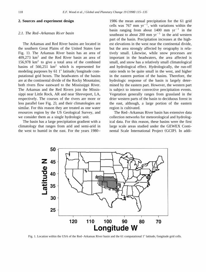
The Arkansas and Red River basins are located inŽthe southern Great Plains of the United States see
.Fig. 1 . The Arkansas River basin has an area of409,273 km2 and the Red River basin an area of156,978 km2 to give a total area of the combinedbasins of 566,251 km2 which is represented formodeling purposes by 61 18 latituderlongitude com-putational grid boxes. The headwaters of the basinsare at the continental divide of the Rocky Mountains;both rivers flow eastward to the Mississippi River.The Arkansas and the Red Rivers join the Missis-sippi near Little Rock, AR and near Shreveport, LA,respectively. The courses of the rivers are more or
Ž .less parallel see Fig. 2 , and their climatologies aresimilar. For this reason they are treated as one waterresources region by the US Geological Survey, andwe consider them as a single hydrologic unit.
The basin has a large precipitation gradient with aclimatology that ranges from arid and semi-arid inthe west to humid in the east. For the years 1980–
1986 the mean annual precipitation for the 61 gridcells was 767 mm yry1, with variations within thebasin ranging from about 1400 mm yry1 in thesoutheast to about 200 mm yry1 in the arid westernpart of the basin. Precipitation increases at the high-est elevations in the west near the continental divide,but the area strongly affected by orography is rela-tively small. Likewise, while snow processes areimportant in the headwaters, the area affected issmall, and snow has a relatively small climatologicaland hydrological effect. Hydrologically, the run-offratio tends to be quite small in the west, and higherin the eastern portion of the basins. Therefore, thehydrologic response of the basin is largely deter-mined by the eastern part. However, the western partis subject to intense convective precipitation events.Vegetation generally ranges from grassland in thedrier western parts of the basin to deciduous forest inthe east, although, a large portion of the easternregion is cultivated.
The Red–Arkansas River basin has extensive datacollection networks for meteorological and hydrolog-ical data. For this reason, these basins were the firstlarge scale areas studied under the GEWEX Conti-
Ž .nental Scale International Project GCIP . In addi-
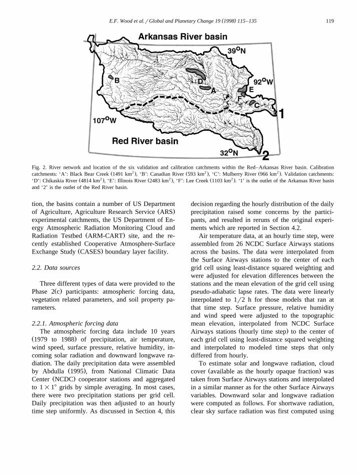
Fig. 1. Location within the USA of the Red–Arkansas River basin and the 61 computational 18 latituderlongitude grid cells.
( )E.F. Wood et al.rGlobal and Planetary Change 19 1998 115–135 119
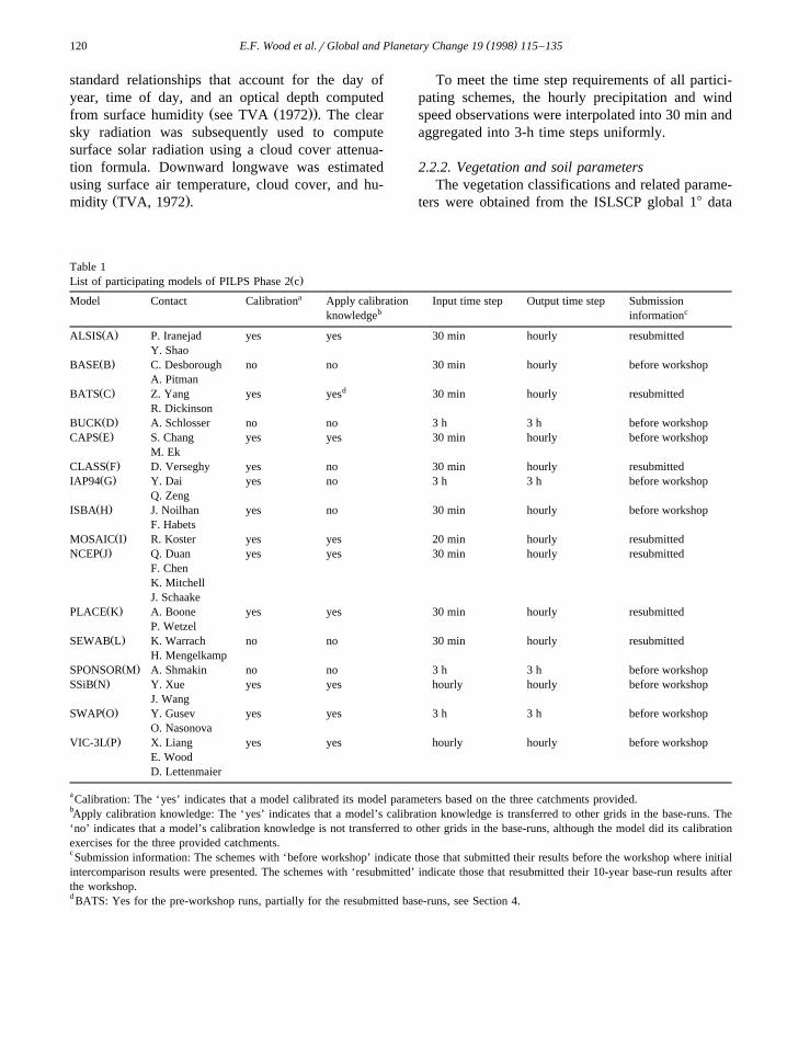
Fig. 2. River network and location of the six validation and calibration catchments within the Red–Arkansas River basin. CalibrationŽ 2 . Ž 2 . Ž 2 .catchments: ‘A’: Black Bear Creek 1491 km , ‘B’: Canadian River 593 km , ‘C’: Mulberry River 966 km . Validation catchments:
Ž 2 . Ž 2 . Ž 2 .‘D’: Chikaskia River 4814 km , ‘E’: Illinois River 2483 km , ‘F’: Lee Creek 1103 km . ‘1’ is the outlet of the Arkansas River basinand ‘2’ is the outlet of the Red River basin.
tion, the basins contain a number of US DepartmentŽ .of Agriculture, Agriculture Research Service ARS
experimental catchments, the US Department of En-ergy Atmospheric Radiation Monitoring Cloud and
Ž .Radiation Testbed ARM-CART site, and the re-cently established Cooperative Atmosphere-Surface
Ž .Exchange Study CASES boundary layer facility.
2.2. Data sources
Three different types of data were provided to theŽ .Phase 2 c participants: atmospheric forcing data,
vegetation related parameters, and soil property pa-rameters.
2.2.1. Atmospheric forcing dataThe atmospheric forcing data include 10 years
Ž .1979 to 1988 of precipitation, air temperature,wind speed, surface pressure, relative humidity, in-coming solar radiation and downward longwave ra-diation. The daily precipitation data were assembled
Ž .by Abdulla 1995 , from National Climatic DataŽ .Center NCDC cooperator stations and aggregated
to 1=18 grids by simple averaging. In most cases,there were two precipitation stations per grid cell.Daily precipitation was then adjusted to an hourlytime step uniformly. As discussed in Section 4, this
decision regarding the hourly distribution of the dailyprecipitation raised some concerns by the partici-pants, and resulted in reruns of the original experi-ments which are reported in Section 4.2.
Air temperature data, at an hourly time step, wereassembled from 26 NCDC Surface Airways stationsacross the basins. The data were interpolated fromthe Surface Airways stations to the center of eachgrid cell using least-distance squared weighting andwere adjusted for elevation differences between thestations and the mean elevation of the grid cell usingpseudo-adiabatic lapse rates. The data were linearlyinterpolated to 1r2 h for those models that ran atthat time step. Surface pressure, relative humidityand wind speed were adjusted to the topographicmean elevation, interpolated from NCDC Surface
Ž .Airways stations hourly time step to the center ofeach grid cell using least-distance squared weightingand interpolated to modeled time steps that onlydiffered from hourly.
To estimate solar and longwave radiation, cloudŽ .cover available as the hourly opaque fraction was
taken from Surface Airways stations and interpolatedin a similar manner as for the other Surface Airwaysvariables. Downward solar and longwave radiationwere computed as follows. For shortwave radiation,clear sky surface radiation was first computed using
( )E.F. Wood et al.rGlobal and Planetary Change 19 1998 115–135120
standard relationships that account for the day ofyear, time of day, and an optical depth computed
Ž Ž ..from surface humidity see TVA 1972 . The clearsky radiation was subsequently used to computesurface solar radiation using a cloud cover attenua-tion formula. Downward longwave was estimatedusing surface air temperature, cloud cover, and hu-
Ž .midity TVA, 1972 .
To meet the time step requirements of all partici-pating schemes, the hourly precipitation and windspeed observations were interpolated into 30 min andaggregated into 3-h time steps uniformly.
2.2.2. Vegetation and soil parametersThe vegetation classifications and related parame-
ters were obtained from the ISLSCP global 18 data
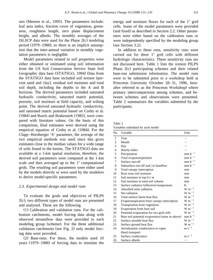
Table 1Ž .List of participating models of PILPS Phase 2 c
aModel Contact Calibration Apply calibration Input time step Output time step Submissionb cknowledge information
Ž .ALSIS A P. Iranejad yes yes 30 min hourly resubmittedY. Shao
Ž .BASE B C. Desborough no no 30 min hourly before workshopA. Pitman
dŽ .BATS C Z. Yang yes yes 30 min hourly resubmittedR. Dickinson
Ž .BUCK D A. Schlosser no no 3 h 3 h before workshopŽ .CAPS E S. Chang yes yes 30 min hourly before workshop
M. EkŽ .CLASS F D. Verseghy yes no 30 min hourly resubmittedŽ .IAP94 G Y. Dai yes no 3 h 3 h before workshop
Q. ZengŽ .ISBA H J. Noilhan yes no 30 min hourly before workshop
F. HabetsŽ .MOSAIC I R. Koster yes yes 20 min hourly resubmitted
Ž .NCEP J Q. Duan yes yes 30 min hourly resubmittedF. ChenK. MitchellJ. Schaake
Ž .PLACE K A. Boone yes yes 30 min hourly resubmittedP. Wetzel
Ž .SEWAB L K. Warrach no no 30 min hourly resubmittedH. Mengelkamp
Ž .SPONSOR M A. Shmakin no no 3 h 3 h before workshopŽ .SSiB N Y. Xue yes yes hourly hourly before workshop
J. WangŽ .SWAP O Y. Gusev yes yes 3 h 3 h before workshop
O. NasonovaŽ .VIC-3L P X. Liang yes yes hourly hourly before workshop
E. WoodD. Lettenmaier
aCalibration: The ‘yes’ indicates that a model calibrated its model parameters based on the three catchments provided.bApply calibration knowledge: The ‘yes’ indicates that a model’s calibration knowledge is transferred to other grids in the base-runs. The‘no’ indicates that a model’s calibration knowledge is not transferred to other grids in the base-runs, although the model did its calibrationexercises for the three provided catchments.cSubmission information: The schemes with ‘before workshop’ indicate those that submitted their results before the workshop where initialintercomparison results were presented. The schemes with ‘resubmitted’ indicate those that resubmitted their 10-year base-run results afterthe workshop.d BATS: Yes for the pre-workshop runs, partially for the resubmitted base-runs, see Section 4.
( )E.F. Wood et al.rGlobal and Planetary Change 19 1998 115–135 121
Ž .sets Meesen et al., 1995 . The parameters include:leaf area index, fraction cover of vegetation, green-ness, roughness length, zero plane displacementheight, and albedo. The monthly averages of the
Ž .ISLSCP data were used for the Phase 2 c modelingŽ .period 1979–1988 , so there is an implicit assump-
tion that the inter-annual variation in monthly vege-tation parameters is negligible.
Model parameters related to soil properties wereeither obtained or estimated using soil informationfrom the US Soil Conservation Service State Soil
Ž .Geographic data base STATSGO, 1994 Data fromŽthe STATSGO data base included soil texture per-
.cent sand and clay , residual soil moisture and totalsoil depth, including the depths to the A and Bhorizons. The derived parameters included saturatedhydraulic conductivity, saturated matric potential,porosity, soil moisture at field capacity, and wiltingpoint. The derived saturated hydraulic conductivity,and saturated matric potential based on Cosby et al.Ž . Ž .1984 and Rawls and Brakensiek 1985 , were com-pared with literature values. On the basis of thiscomparison, final estimates were derived using the
Ž .empirical equation of Cosby et al. 1984 . For theClapp–Hornberger ‘b’ parameter, the average of thetwo empirical methods was used since this givesestimates close to the median values for a wide rangeof soils found in the basins. The STATSGO data areavailable at a 1-km spatial resolution, therefore, thederived soil parameters were computed at the 1-kmscale and then averaged up to the 18 computationalgrids. The resulting soil parameters were either usedby the models directly or were used by the modelersto derive model-specific parameters.
2.3. Experimental design and model runs
To evaluate the goals and objectives of PILPSŽ .2 c , two different types of model runs are presented
and analyzed. These are the following.Ž .1 Calibration and validation runs. For the cali-
bration catchments, model forcing data along withobserved streamflow data were provided to each
Ž .modeling group scheme . For the three additionalŽ .validation catchments see Fig. 2 only model forc-
ing data were provided.Ž .2 Base-runs. For these, the models used 10
Ž .years 1979–1988 of forcing data to simulate the
energy and moisture fluxes for each of the 18 gridcells. Some of the model parameters were providedŽ .and fixed as described in Section 2.2. Other param-eters were either based on the calibration runs orwere independently specified by the modeling groupŽ .see Section 3.2 .
In addition to these runs, sensitivity runs werecarried out for three 18 grid cells with differenthydrologic characteristics. These sensitivity runs arenot discussed here. Table 1 lists the sixteen PILPS
Ž .Phase 2 c participating schemes and their relatedbase-run submission information. The model runswere to be submitted prior to a workshop held at
ŽPrinceton University October 28–31, 1996, here-.after referred to as the Princeton Workshop where
primary intercomparisons among schemes, and be-tween schemes and observations were presented.Table 2 summarizes the variables submitted by theparticipants.
Table 2Variables submitted by each model
No. Variable Unit
1 Year y2 Month y3 Day y4 Hourly-index y
y15 Precipitation mm hy16 Total evapotranspiration mm hy17 Surface run-off mm hy18 Subsurface run-off andror baseflow mm h
9 Total canopy interception mm10 Root zone soil moisture mm11 Soil moisture in top 0.1 m mm12 Soil moisture in total soil column mm
Ž .13 Surface radiative effective temperature Ky214 Absorbed solar radiation W my215 Net radiation W my216 Total surface latent heat flux W my217 Evapotranspiration from canopy interception W my218 Transpiration from vegetation W my219 Evaporation from bare soil W my220 Potential evaporation for two grid cells W my1Ž .21 Bare soil potential evaporation same as above mm h
y222 Surface sensible heat flux W my223 Surface ground heat flux W m
y124 Aerodynamic conductance to vapor m sŽ .heat transport
y125 Surface conductance m s26 Surface albedo y
( )E.F. Wood et al.rGlobal and Planetary Change 19 1998 115–135122
As will be discussed in Section 4, seven schemesresubmitted their base-run results after the workshopfor various reasons. The results presented in thispaper are based on the most recently submitted runsfor these models. For the other nine schemes, theanalysis is based on the runs submitted before the
Žworkshop with the exception of additional runsdescribed in Section 4 designed to test the effect of
.the diurnal precipitation pattern . The schemes whosebase-run results were resubmitted after the workshopare ALSIS, BATS, CLASS, MOSAIC, NCEP,PLACE, and SEWAB. The reasons for the resubmis-sions are briefly summarized in Section 4 wherecomparisons between the original and resubmittedruns are made for the mean annual water and energybalance, and mean monthly run-off and evaporation.
3. Analysis and results
3.1. Calibration–Õalidation results
The purpose of the calibration–validation runswas to test the ability of schemes to calibrate theirparameters using data from smaller catchments and
to transfer this information to other similarly sizedcatchments and to larger computational grids. Theruns are intended to provide insight as to whethersuch parameter calibration, widely used in hydrologi-cal modeling, would improve the performance of theland-surface schemes, even when the land-surfaceschemes use ‘physically-based’ parameters that intheory can be estimated from land cover character-istics such as soil or vegetation data. These calibra-tion–validation runs are a first attempt within PILPSto address this issue.
The calibration and validation runs consisted oftwo parts. In the calibration runs, model forcing datafor three catchments were provided along with ob-served streamflow data. These catchments, shown in
Ž 2Fig. 2, were Black Bear Creek 1491 km , desig-Ž 2nated by ‘A’ in Fig. 2, the Canadian River 593 km ,
. Ž 2designated ‘B’ and the Mulberry River 966 km ,
.designated ‘C’ . For these catchments, the modelswere first run using their ‘standard’ parameter val-ues. Then, using the streamflow data, adjustmentswere allowed to specific model parameters to im-prove the comparison between predicted and ob-served streamflow. The modeling groups provided
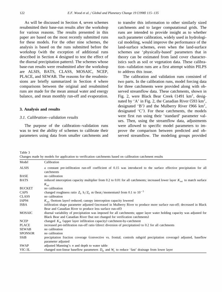
Table 3Changes made by models for application to verification catchments based on calibration catchment results
Model Calibration
ALSIS a constant pre-infiltration run-off coefficient of 0.15 was introduced to the surface effective precipitation for allcatchments
BASE no calibrationBATS reduced interception capacity multiplier from 0.2 to 0.01 for all catchments; increased lower layer K to match surfacesat
Ksat
BUCKET no calibrationy5Ž .CAPS changed roughness ratio Z hrZ m heatrmomentum from 0.1 to 100 0
CLASS no calibrationŽ .IAP94 K bottom layer reduced; canopy interception capacity loweredsat
ŽISBA infiltration shape parameter adjusted increased in Mulberry River to produce more surface run-off; decreased in Black.Bear and Canadian River to produce less surface run-off
MOSAIC diurnal variability of precipitation was imposed for all catchments; upper layer water holding capacity was adjusted forŽ .Black Bear and Canadian River but not changed for verification catchments
Ž .NCEP changed K upper layer infiltration capacity catchment-by-catchmentdtŽ .PLACE increased pre-infiltration run-off ratio direct diversion of precipitation to 0.2 for all catchments
SEWAB no calibrationSPONSOR no calibration
Ž .SSiB precipitation fraction coverage convective vs. frontal; controls subgrid precipitation coverage adjusted, baseflowparameter adjusted
SWAP adjusted Manning’s n and depth to water tableVIC-3L changed non-linear baseflow parameters D and W to reduce ‘fast’ drainage from lower layerm s
( )E.F. Wood et al.rGlobal and Planetary Change 19 1998 115–135 123
the organizers with the model-derived streamflowtime series before and after calibration.
For three additional validation catchments onlyforcing data were provided. These catchments were
Ž 2the Chikaskia River 4814 km , designated ‘D’ in. Ž 2 .Fig. 2 , the Illinois River 2483 km , designated ‘E’
Ž 2 .and Lee Creek 1103 km , designated ‘F’ , whichserved as the validation catchments. The modelinggroups were asked to summarize what model param-eters they adjusted in the calibration process. Itshould be noted that some groups varied parametersthat should have remained fixed, so the potential forimprovements due to calibration may be somewhatdifferent than indicated in the results. Table 3 indi-cates how each model’s parameters were adjustedduring the calibration runs.
The range of approaches to parameter calibrationcan be grouped into four classes.
Ž . Ž1 Six models ALSIS, ISBA, NCEP, PLACE,.SSiB and VIC-3L empirically adjusted the model
parameters so as to fit the calibration data.
Ž . Ž2 Six models BATS, CAPS, IAP94, MOSAIC,.SSiB, SWAP varied their internal representation of
various processes, using their knowledge about modelsensitivities, so as to fit the calibration data.
Ž . Ž .3 One model MOSAIC varied the precipitationforcing diurnal pattern, which was assumed uniform
Ž .in the original data set see Section 4.2 , by imposinga new daily cycle.
Ž . Ž4 Five models BASE, BUCK, CLASS, SE-.WAB, SPONSOR did not calibrate.
SSiB appears in two groups because it adjusted itsŽ .baseflow parameter group 1 and adjusted the pa-
rameter which describes the spatial heterogeneity ofŽ .precipitation group 2 .
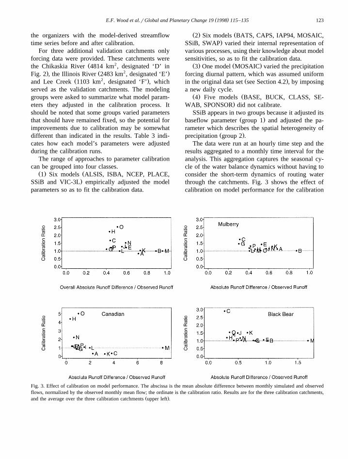
The data were run at an hourly time step and theresults aggregated to a monthly time interval for theanalysis. This aggregation captures the seasonal cy-cle of the water balance dynamics without having toconsider the short-term dynamics of routing waterthrough the catchments. Fig. 3 shows the effect ofcalibration on model performance for the calibration
Fig. 3. Effect of calibration on model performance. The abscissa is the mean absolute difference between monthly simulated and observedflows, normalized by the observed monthly mean flow; the ordinate is the calibration ratio. Results are for the three calibration catchments,
Ž .and the average over the three calibration catchments upper left .
( )E.F. Wood et al.rGlobal and Planetary Change 19 1998 115–135124
catchments. The upper left panel shows results aver-aged over the three calibration catchments, while theother three panels show results for the individualcalibration catchments. The horizontal axis indicatesthe average monthly absolute deviation, normalizedby observed streamflow, after calibration. The verti-cal axis, labeled the calibration ratio, is the ratio ofthe mean absolute error before and after calibration,and indicates the degree of improvement in modelperformance due to calibration. Values less than 1.0indicate poorer performance after calibration. Forsome models the improvement is by a factor of
Ž .almost 5 SWAP and ISBA . The improvement wasnot consistent across the three catchments. For exam-ple, calibration significantly improved BATS’ per-formance on the Black Bear catchment, improved itsomewhat on the Mulberry, and degraded its perfor-mance on the Canadian. For reference, those modelsthat did not calibrate but submitted uncalibrated runs
Ž .are shown BASE, ‘B’, and SPONSOR, ‘M’ andplotted on the horizontal line, 1.0. Overall, calibra-
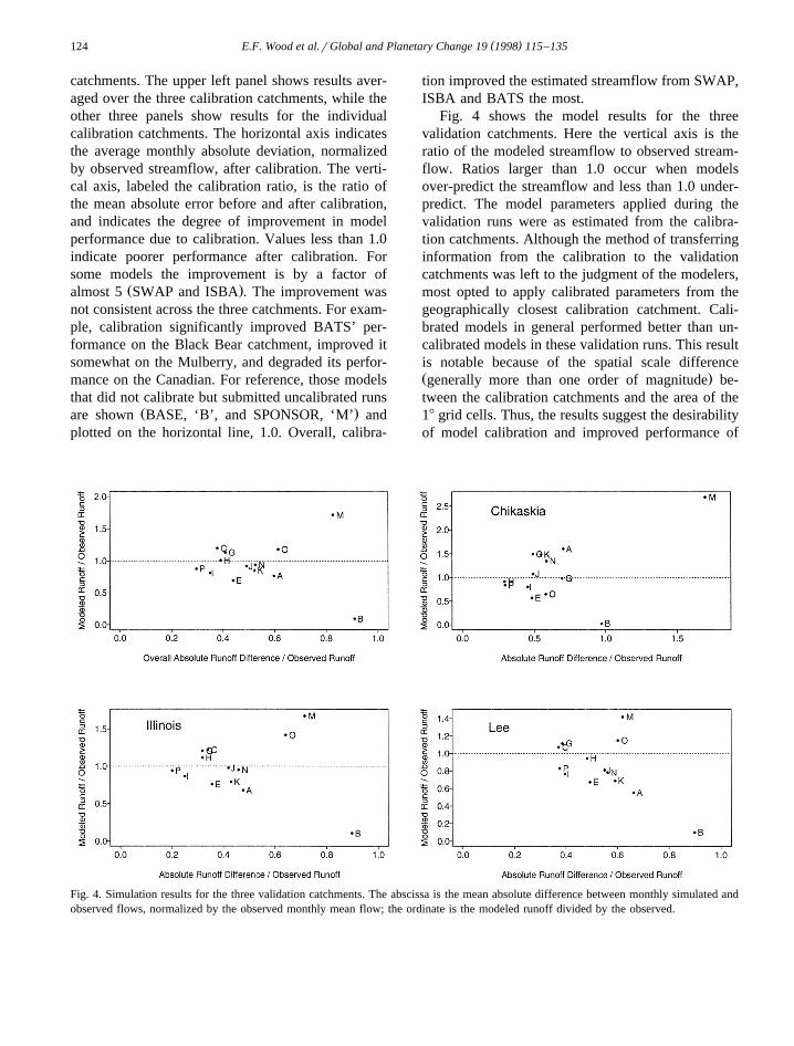
tion improved the estimated streamflow from SWAP,ISBA and BATS the most.
Fig. 4 shows the model results for the threevalidation catchments. Here the vertical axis is theratio of the modeled streamflow to observed stream-flow. Ratios larger than 1.0 occur when modelsover-predict the streamflow and less than 1.0 under-predict. The model parameters applied during thevalidation runs were as estimated from the calibra-tion catchments. Although the method of transferringinformation from the calibration to the validationcatchments was left to the judgment of the modelers,most opted to apply calibrated parameters from thegeographically closest calibration catchment. Cali-brated models in general performed better than un-calibrated models in these validation runs. This resultis notable because of the spatial scale differenceŽ .generally more than one order of magnitude be-tween the calibration catchments and the area of the18 grid cells. Thus, the results suggest the desirabilityof model calibration and improved performance of
Fig. 4. Simulation results for the three validation catchments. The abscissa is the mean absolute difference between monthly simulated andobserved flows, normalized by the observed monthly mean flow; the ordinate is the modeled runoff divided by the observed.
( )E.F. Wood et al.rGlobal and Planetary Change 19 1998 115–135 125
land-surface schemes. It is recognized that theseresults are not definitive and that PILPS shouldconsider organizing more extensive calibration–validation experiments.
3.2. Approaches to transferring information fromcatchments to grid-scale
Each of the modeling groups was asked to sum-marize how information from the test catchmentswas transferred to the grid scale. The responses aresummarized in Table 4. Again, it should be notedthat during the calibration runs some modelers variedparameters that should have remained fixed accord-ing to the guidelines provided by the experimentorganizers. It is unclear how these varied parameters,when transferred to the 61 grid boxes, influenced
Ž .their results. In addition, some modelers e.g., ISBAchose not to use the calibrated parameters in the10-year base-runs. A number of important issuesremain to be resolved with respect to calibration ofland-surface models-most importantly, how manycalibration basins are necessary, what objective func-tions should be used for model calibration, and howto transfer calibration information between scales
Ži.e., from intermediate scale catchment to the re-.gion .
3.3. Subsection intercomparisons oÕer the 10-yearbase-runs
In conducting the base-runs, each model initial-ized its soil moisture at half of its soil saturation foreach soil moisture layer. The canopy interceptionwas initialized at zero for all models. The soil andsurface temperatures were initialized to the air tem-perature at the first modeling time step. Each modelwas run using the 10-year forcing data set with thesame initial condition. The required output variablesat each hourly time step for each of the 61 grid cellsare listed in Table 2, which include model-computedfluxes, state variables, and selected forcings. For theschemes which do not have an easy way to outputthe required variables as listed in Table 2, y999 wasreported instead.
Ž .Ten years of forcing data 1979–1988 were usedto conduct the base-run simulations. The 1st year,1979, was eliminated from the analysis to removeany initialization effects. In addition, there wereconcerns about some of the data used for the atmo-
Table 4Parameter changes and information transfer for the base-runs using calibration–validation run results
Model Changes applied to regional scale
ALSIS noneBASE did not calibrateBATS none in pre-workshop runs, used interception capacitys0.2 mm in the base-run resubmissionBUCKET did not calibrate
Ž .CAPS changed roughness ratio momentum to heat everywhere same as calibration catchments; set zero plane displacementheight to zero everywhere
CLASS did not calibrateIAP94 noneISBA noneMOSAIC areal storm fraction from the calibration catchments
Ž . Ž . Ž .NCEP changed K upper layer infiltration coefficient by classifying grid cells according to precipitation climatology as adtŽ . Ž .aridrsemi-arid; b semi-humid; c humid; applying calibration changes from Canadian River; Black Bear Creek,
Mulberry River to a, b, c, respectivelyPLACE noneSEWAB did not calibrateSPONSOR did not calibrateSSiB applied change in proportion of convective vs. large scale precipitation uniformly to entire regionSWAP linearly interpolated depth to water table from calibration catchments; applied geometric mean of Manning’s n from
calibration catchments uniformly to entire regionVIC-3L scale soil properties; adjusted W based on grid scale field capacitiess
( )E.F. Wood et al.rGlobal and Planetary Change 19 1998 115–135126
spheric budget computations which provided the re-gional evapotranspiration estimates. Therefore, onlythe estimates from 1980 to 1986 from each schemewere used in the analyses presented here.
3.4. Water and energy balance checks
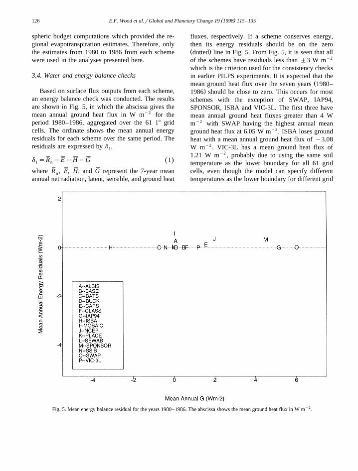
Based on surface flux outputs from each scheme,an energy balance check was conducted. The resultsare shown in Fig. 5, in which the abscissa gives themean annual ground heat flux in W my2 for theperiod 1980–1986, aggregated over the 61 18 gridcells. The ordinate shows the mean annual energyresiduals for each scheme over the same period. Theresiduals are expressed by d ,1
d sR yEyHyG 1Ž .1 n
where R , E, H, and G represent the 7-year meann
annual net radiation, latent, sensible, and ground heat
fluxes, respectively. If a scheme conserves energy,then its energy residuals should be on the zeroŽ .dotted line in Fig. 5. From Fig. 5, it is seen that allof the schemes have residuals less than "3 W my2
which is the criterion used for the consistency checksin earlier PILPS experiments. It is expected that the
Žmean ground heat flux over the seven years 1980–.1986 should be close to zero. This occurs for most
schemes with the exception of SWAP, IAP94,SPONSOR, ISBA and VIC-3L. The first three havemean annual ground heat fluxes greater than 4 Wmy2 with SWAP having the highest annual meanground heat flux at 6.05 W my2 . ISBA loses groundheat with a mean annual ground heat flux of y3.08W my2 . VIC-3L has a mean ground heat flux of1.21 W my2 , probably due to using the same soiltemperature as the lower boundary for all 61 gridcells, even though the model can specify differenttemperatures as the lower boundary for different grid
Fig. 5. Mean energy balance residual for the years 1980–1986. The abscissa shows the mean ground heat flux in W my2 .
( )E.F. Wood et al.rGlobal and Planetary Change 19 1998 115–135 127
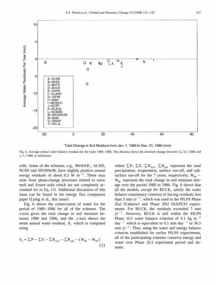
Fig. 6. Average annual water balance residual for the years 1980–1986. The abscissa shows the moisture change between 12r31r1986 and1r1r1980 in millimeter.
cells. Some of the schemes, e.g., MOSAIC, ALSIS,NCEP and SPONSOR, have slightly positive annualenergy residuals of about 0.5 W my2 . These mayarise from phase-change processes related to snowmelt and frozen soils which are not completely ac-
Ž .counted for in Eq. 1 . Additional discussion of thisissue can be found in the energy flux companion
Ž .paper Liang et al., this issue .Fig. 6 shows the conservation of water for the
period of 1980–1986 for all of the schemes. Thex-axis gives the total change in soil moisture be-tween 1980 and 1986, and the y-axis shows themean annual water residual, d which is computed2
using
d sÝPyÝEyÝR yÝR y W yWŽ .2 surf sub 86 80
2Ž .
where ÝP, ÝE, ÝR , ÝR represent the totalsurf sub
precipitation, evaporation, surface run-off, and sub-surface run-off for the 7 years, respectively; W y86
W represent the total change in soil moisture stor-80
age over the period 1980 to 1986. Fig. 6 shows thatall the models, except for BUCK, satisfy the waterbalance consistency criterion of having residuals lessthan 3 mm yry1, which was used in the PILPS PhaseŽ . Ž . Ž . Ž .2 a Cabauw and Phase 2 b HAPEX experi-
ments. For BUCK, the residuals exceeded 7 mmyry1. However, BUCK is still within the PILPS
Ž . y2Phase 1 c water balance criterion of 0.1 kg mdayy1 which is equivalent to 0.1 mm dayy1 or 36.5mm yry1. Thus, using the water and energy balancecriterion established for earlier PILPS experiments,all of the participating schemes conserve energy and
Ž .water over Phase 2 c experiment period and do-main.
( )E.F. Wood et al.rGlobal and Planetary Change 19 1998 115–135128
3.5. Mean annual energy and water balance inter-comparisons
Ž .The initial analysis of Phase 2 c model runs,after checking that the schemes conserve energy andwater, focuses on the long-term components of thebalances. For the energy balance, this is the meanannual sensible heat and latent heat which is bal-anced by the net radiation assuming a mean annualground heat flux of zero and an energy conservingscheme. For the water balance, the mean annualprecipitation is balanced by the mean annual run-offand evapotranspiration, again assuming no long termchange in soil moisture storage and a water conserv-ing scheme.
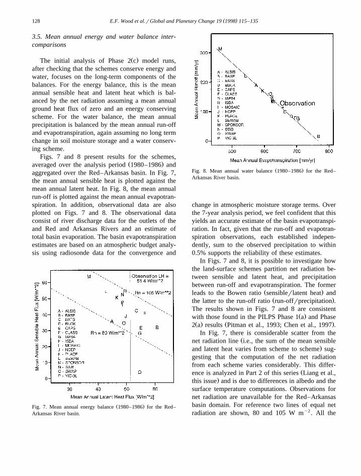
Figs. 7 and 8 present results for the schemes,Ž .averaged over the analysis period 1980–1986 and
aggregated over the Red–Arkansas basin. In Fig. 7,the mean annual sensible heat is plotted against themean annual latent heat. In Fig. 8, the mean annualrun-off is plotted against the mean annual evapotran-spiration. In addition, observational data are alsoplotted on Figs. 7 and 8. The observational dataconsist of river discharge data for the outlets of theand Red and Arkansas Rivers and an estimate oftotal basin evaporation. The basin evapotranspirationestimates are based on an atmospheric budget analy-sis using radiosonde data for the convergence and
Ž .Fig. 7. Mean annual energy balance 1980–1986 for the Red–Arkansas River basin.
Ž .Fig. 8. Mean annual water balance 1980–1986 for the Red–Arkansas River basin.
change in atmospheric moisture storage terms. Overthe 7-year analysis period, we feel confident that thisyields an accurate estimate of the basin evapotranspi-ration. In fact, given that the run-off and evapotran-spiration observations, each established indepen-dently, sum to the observed precipitation to within0.5% supports the reliability of these estimates.
In Figs. 7 and 8, it is possible to investigate howthe land-surface schemes partition net radiation be-tween sensible and latent heat, and precipitationbetween run-off and evapotranspiration. The former
Ž .leads to the Bowen ratio sensiblerlatent heat andŽ .the latter to the run-off ratio run-offrprecipitation .
The results shown in Figs. 7 and 8 are consistentŽ .with those found in the PILPS Phase 1 a and Phase
Ž . Ž .2 a results Pitman et al., 1993; Chen et al., 1997 .In Fig. 7, there is considerable scatter from the
Žnet radiation line i.e., the sum of the mean sensible.and latent heat varies from scheme to scheme sug-
gesting that the computation of the net radiationfrom each scheme varies considerably. This differ-
Žence is analyzed in Part 2 of this series Liang et al.,.this issue and is due to differences in albedo and the
surface temperature computations. Observations fornet radiation are unavailable for the Red–Arkansasbasin domain. For reference two lines of equal netradiation are shown, 80 and 105 W my2 . All the
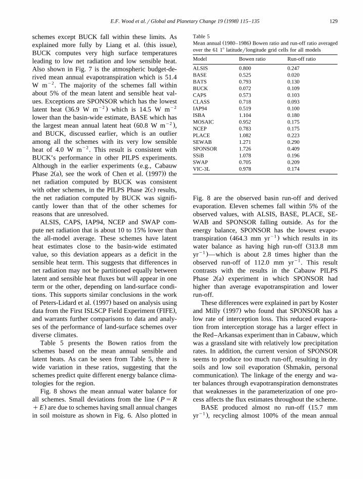
( )E.F. Wood et al.rGlobal and Planetary Change 19 1998 115–135 129
schemes except BUCK fall within these limits. AsŽ .explained more fully by Liang et al. this issue ,
BUCK computes very high surface temperaturesleading to low net radiation and low sensible heat.Also shown in Fig. 7 is the atmospheric budget-de-rived mean annual evapotranspiration which is 51.4W my2 . The majority of the schemes fall withinabout 5% of the mean latent and sensible heat val-ues. Exceptions are SPONSOR which has the lowest
Ž y2 . y2latent heat 36.9 W m which is 14.5 W mlower than the basin-wide estimate, BASE which has
Ž y2 .the largest mean annual latent heat 60.8 W m ,and BUCK, discussed earlier, which is an outlieramong all the schemes with its very low sensibleheat of 4.0 W my2 . This result is consistent withBUCK’s performance in other PILPS experiments.
ŽAlthough in the earlier experiments e.g., CabauwŽ . Ž ..Phase 2 a , see the work of Chen et al. 1997 the
net radiation computed by BUCK was consistentŽ .with other schemes, in the PILPS Phase 2 c results,
the net radiation computed by BUCK was signifi-cantly lower than that of the other schemes forreasons that are unresolved.
ALSIS, CAPS, IAP94, NCEP and SWAP com-pute net radiation that is about 10 to 15% lower thanthe all-model average. These schemes have latentheat estimates close to the basin-wide estimatedvalue, so this deviation appears as a deficit in thesensible heat term. This suggests that differences innet radiation may not be partitioned equally betweenlatent and sensible heat fluxes but will appear in oneterm or the other, depending on land-surface condi-tions. This supports similar conclusions in the work
Ž .of Peters-Lidard et al. 1997 based on analysis usingŽ .data from the First ISLSCP Field Experiment FIFE ,
and warrants further comparisons to data and analy-ses of the performance of land-surface schemes overdiverse climates.
Table 5 presents the Bowen ratios from theschemes based on the mean annual sensible andlatent heats. As can be seen from Table 5, there iswide variation in these ratios, suggesting that theschemes predict quite different energy balance clima-tologies for the region.
Fig. 8 shows the mean annual water balance forŽall schemes. Small deviations from the line PsR
.qE are due to schemes having small annual changesin soil moisture as shown in Fig. 6. Also plotted in
Table 5Ž .Mean annual 1980–1986 Bowen ratio and run-off ratio averaged
over the 61 18 latituderlongitude grid cells for all models
Model Bowen ratio Run-off ratio
ALSIS 0.800 0.247BASE 0.525 0.020BATS 0.793 0.130BUCK 0.072 0.109CAPS 0.573 0.103CLASS 0.718 0.093IAP94 0.519 0.100ISBA 1.104 0.180MOSAIC 0.952 0.175NCEP 0.783 0.175PLACE 1.082 0.223SEWAB 1.271 0.290SPONSOR 1.726 0.409SSiB 1.078 0.196SWAP 0.705 0.209VIC-3L 0.978 0.174
Fig. 8 are the observed basin run-off and derivedevaporation. Eleven schemes fall within 5% of theobserved values, with ALSIS, BASE, PLACE, SE-WAB and SPONSOR falling outside. As for theenergy balance, SPONSOR has the lowest evapo-
Ž y1 .transpiration 464.3 mm yr which results in itsŽwater balance as having high run-off 313.8 mm
y1 .yr —which is about 2.8 times higher than theobserved run-off of 112.0 mm yry1. This resultcontrasts with the results in the Cabauw PILPS
Ž .Phase 2 a experiment in which SPONSOR hadhigher than average evapotranspiration and lowerrun-off.
These differences were explained in part by KosterŽ .and Milly 1997 who found that SPONSOR has a
low rate of interception loss. This reduced evapora-tion from interception storage has a larger effect inthe Red–Arkansas experiment than in Cabauw, whichwas a grassland site with relatively low precipitationrates. In addition, the current version of SPONSORseems to produce too much run-off, resulting in dry
Žsoils and low soil evaporation Shmakin, personal.communication . The linkage of the energy and wa-
ter balances through evapotranspiration demonstratesthat weaknesses in the parameterization of one pro-cess affects the flux estimates throughout the scheme.
ŽBASE produced almost no run-off 15.7 mmy1 .yr , recycling almost 100% of the mean annual
( )E.F. Wood et al.rGlobal and Planetary Change 19 1998 115–135130
precipitation. Table 5 also lists the run-off ratiosŽ .RrP for the various schemes. Additional analysisregarding the run-off estimates and water balancefrom the schemes is presented in the Part 3 compan-
Ž .ion paper of Lohmann et al. this issue .
4. Post-workshop model re-runs
During the workshop, two issues arose that re-sulted in some of the participants resubmitting thebase-runs. The first issue related to inconsistenciesbetween the experiment’s protocols and the submit-ted runs. In addition, some participants submittedoutput with inadvertent errors, found coding errors intheir models, andror felt that the parameters fromthe calibration–validation were inappropriate for theirschemes. These resubmissions are referred to as the
Ž .resubmitted base-runs see Section 4.1 . The secondissue that arose in the workshop was the use, in the
Ž .original forcing data, of uniform daily averageprecipitation throughout a rain-day, and how thiscould influence the results. Post-workshop modelruns using a precipitation data set that includes theobserved hourly pattern are referred to as the disag-
Ž .gregated precipitation reruns see Section 4.2 . InSections 4.1 and 4.2, we compare the pre- andpost-workshop submissions.
4.1. Resubmitted base-runs
Seven schemes resubmitted the 10-year base-runsafter the workshop: ALSIS, BATS, CLASS, MO-SAIC, NCEP, PLACE and SEWAB. The reasons forthe resubmission are briefly summarized below. AL-SIS resubmitted due to bad soil parameters retainedfrom test runs, resulting in inconsistent results in theearlier submission. This modeling group did notattend the Princeton Workshop.
BATS resubmitted due to deviations of their pro-cedure from the workshop instructions with respectto modification of model parameters during the cali-bration runs, the effect of which was that the inter-ception capacity multiplier was changed from 0.2mm to 0.01 mm. BATS resubmitted using 0.2 mminterception capacity in order to have the same basisfor intercomparisons of the base-runs.
CLASS resubmitted twice. CLASS felt that theŽfirst base-run version with adjusted parameters from
.the calibration run did not correspond to any pub-lished version of CLASS and preferred to resubmitresults using its standard parameter values; i.e., anuncalibrated run. The second resubmission was ow-ing to the discovery of a recently introduced bug inthe surface mixed layer formulation.
ŽMOSAIC originally submitted using with the.permission of the organizers a different diurnal pre-
cipitation pattern. In order to have the same basis forintercomparisons among schemes, MOSAIC resub-
Žmitted the 10-year base-run using uniform daily.average precipitation. In the resubmitted base-runs,
instead of using the calibration data to adjust thetemporal partitioning of precipitation, MOSAIC used
Ž .these data and these data only to calibrate theirareal storm wetting fraction. The calibration–valida-
Ž .tion analysis for MOSAIC see Section 3.1 is basedon the original runs using the non-uniform precipita-tion.
NCEP resubmitted due to a coding error as aresult of code transfer and due to the adjustment of aconstant related to the calculation of potential evapo-transpiration.
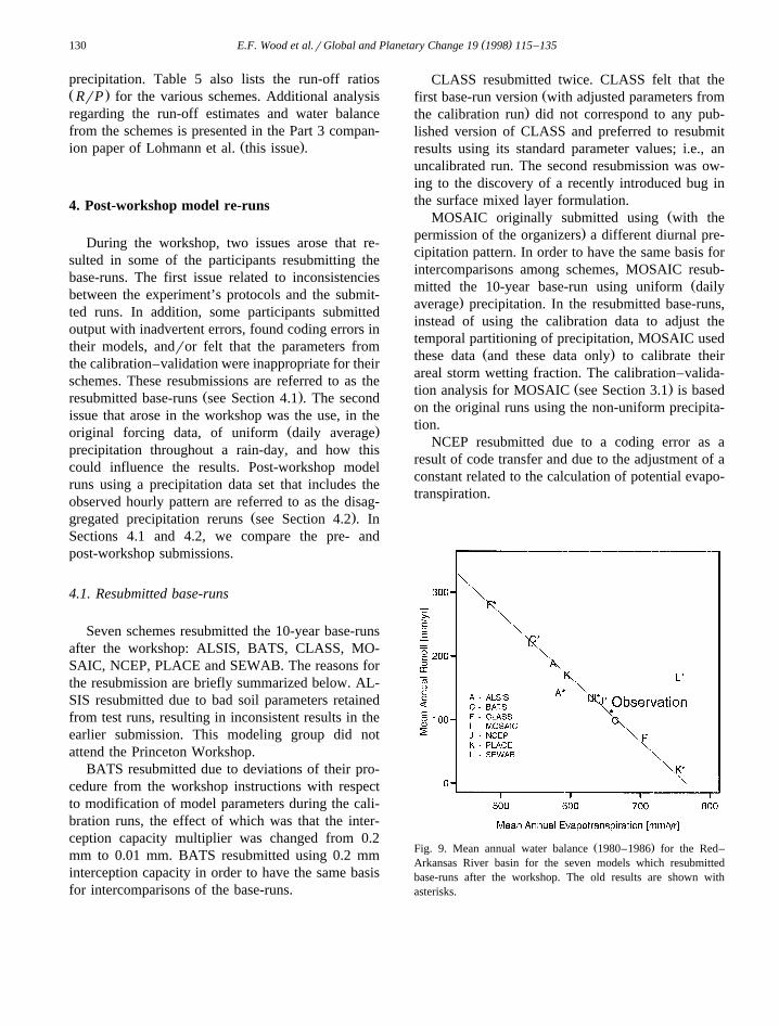
Ž .Fig. 9. Mean annual water balance 1980–1986 for the Red–Arkansas River basin for the seven models which resubmittedbase-runs after the workshop. The old results are shown withasterisks.
( )E.F. Wood et al.rGlobal and Planetary Change 19 1998 115–135 131
PLACE resubmitted due to not using their calibra-tion information in the initial submission. The resub-mission is more consistent by applying knowledgefrom the calibration procedure.
SEWAB resubmitted due to coding errors foundin their canopy evaporation parameterization.
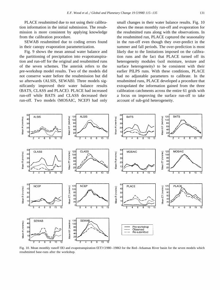
Fig. 9 shows the mean annual water balance andthe partitioning of precipitation into evapotranspira-tion and run-off for the original and resubmitted runsof the seven schemes. The asterisk refers to thepre-workshop model results. Two of the models didnot conserve water before the resubmission but did
Ž .so afterwards ALSIS, SEWAB . Three models sig-nificantly improved their water balance resultsŽ .BATS, CLASS and PLACE . PLACE had increasedrun-off while BATS and CLASS decreased their
Ž .run-off. Two models MOSAIC, NCEP had only
small changes in their water balance results. Fig. 10shows the mean monthly run-off and evaporation forthe resubmitted runs along with the observations. Inthe resubmitted run, PLACE captured the seasonalityin the run-off even though they over-predict in thesummer and fall periods. The over-prediction is mostlikely due to the limitations imposed on the calibra-tion runs and the fact that PLACE turned off its
Žheterogeneity modules soil moisture, texture and.surface heterogeneity to be consistent with their
earlier PILPS runs. With these conditions, PLACEhad no adjustable parameters to calibrate. In theresubmitted runs, PLACE developed a procedure thatextrapolated the information gained from the threecalibration catchments across the entire 61 grids witha focus on improving the surface run-off to takeaccount of sub-grid heterogeneity.
Ž . Ž . Ž .Fig. 10. Mean monthly runoff R and evapotranspiration ET 1980–1986 for the Red–Arkansas River basin for the seven models whichresubmitted base-runs after the workshop.
( )E.F. Wood et al.rGlobal and Planetary Change 19 1998 115–135132
BATS and CLASS improved significantly theirrun-off prediction, especially during the summer, buttended to under-predict spring run-off. ALSIS andSEWAB had poorer run-off results after the resub-mission; ALSIS had a small change to its evapotran-spiration and SEWAB went from over-predictingevapotranspiration to under-predicting. BATS,CLASS, and PLACE all improved their seasonalevapotranspiration. NCEP and MOSAIC showed lit-tle change in their monthly results.
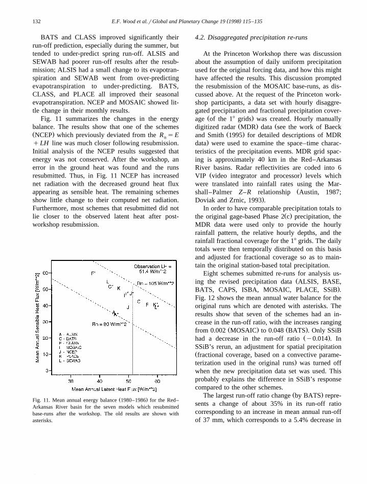
Fig. 11 summarizes the changes in the energybalance. The results show that one of the schemesŽ .NCEP which previously deviated from the R sEn
qLH line was much closer following resubmission.Initial analysis of the NCEP results suggested thatenergy was not conserved. After the workshop, anerror in the ground heat was found and the runsresubmitted. Thus, in Fig. 11 NCEP has increasednet radiation with the decreased ground heat fluxappearing as sensible heat. The remaining schemesshow little change to their computed net radiation.Furthermore, most schemes that resubmitted did notlie closer to the observed latent heat after post-workshop resubmission.
Ž .Fig. 11. Mean annual energy balance 1980–1986 for the Red–Arkansas River basin for the seven models which resubmittedbase-runs after the workshop. The old results are shown withasterisks.
4.2. Disaggregated precipitation re-runs
At the Princeton Workshop there was discussionabout the assumption of daily uniform precipitationused for the original forcing data, and how this mighthave affected the results. This discussion promptedthe resubmission of the MOSAIC base-runs, as dis-cussed above. At the request of the Princeton work-shop participants, a data set with hourly disaggre-gated precipitation and fractional precipitation cover-
Ž .age of the 18 grids was created. Hourly manuallyŽ . Ždigitized radar MDR data see the work of Baeck
Ž .and Smith 1995 for detailed descriptions of MDR.data were used to examine the space–time charac-
teristics of the precipitation events. MDR grid spac-ing is approximately 40 km in the Red–ArkansasRiver basins. Radar reflectivities are coded into 6
Ž .VIP video integrator and processor levels whichwere translated into rainfall rates using the Mar-
Žshall–Palmer Z–R relationship Austin, 1987;.Doviak and Zrnic, 1993 .
In order to have comparable precipitation totals toŽ .the original gage-based Phase 2 c precipitation, the
MDR data were used only to provide the hourlyrainfall pattern, the relative hourly depths, and therainfall fractional coverage for the 18 grids. The dailytotals were then temporally distributed on this basisand adjusted for fractional coverage so as to main-tain the original station-based total precipitation.
Eight schemes submitted re-runs for analysis us-Žing the revised precipitation data ALSIS, BASE,
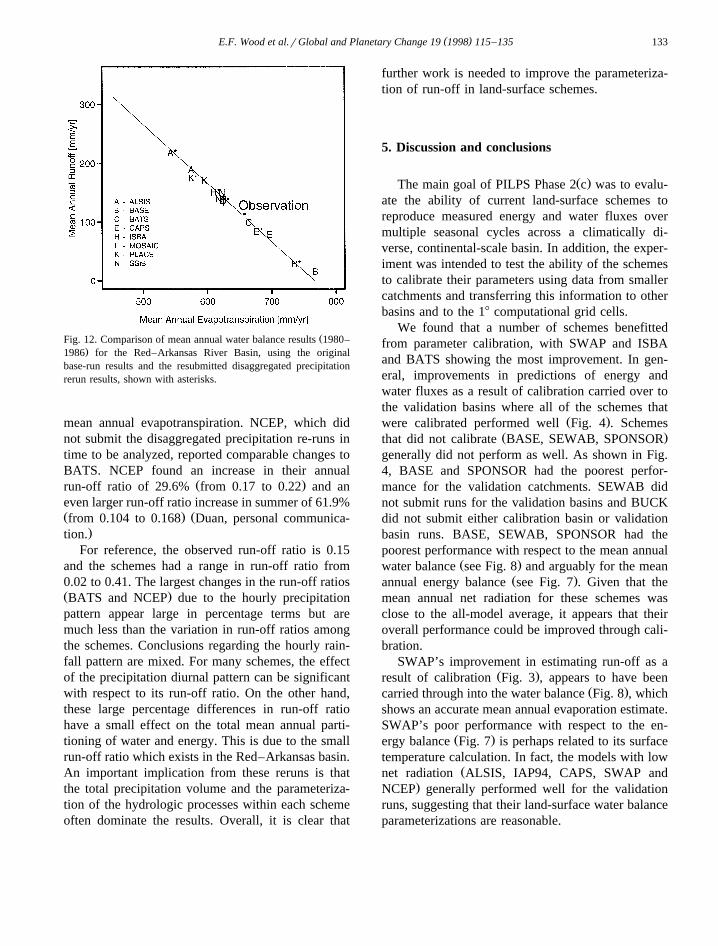
.BATS, CAPS, ISBA, MOSAIC, PLACE, SSiB .Fig. 12 shows the mean annual water balance for theoriginal runs which are denoted with asterisks. Theresults show that seven of the schemes had an in-crease in the run-off ratio, with the increases ranging
Ž . Ž .from 0.002 MOSAIC to 0.048 BATS . Only SSiBŽ .had a decrease in the run-off ratio y0.014 . In
SSiB’s rerun, an adjustment for spatial precipitationŽfractional coverage, based on a convective parame-
.terization used in the original runs was turned offwhen the new precipitation data set was used. Thisprobably explains the difference in SSiB’s responsecompared to the other schemes.
Ž .The largest run-off ratio change by BATS repre-sents a change of about 35% in its run-off ratiocorresponding to an increase in mean annual run-offof 37 mm, which corresponds to a 5.4% decrease in
( )E.F. Wood et al.rGlobal and Planetary Change 19 1998 115–135 133
ŽFig. 12. Comparison of mean annual water balance results 1980–.1986 for the Red–Arkansas River Basin, using the original
base-run results and the resubmitted disaggregated precipitationrerun results, shown with asterisks.
mean annual evapotranspiration. NCEP, which didnot submit the disaggregated precipitation re-runs intime to be analyzed, reported comparable changes toBATS. NCEP found an increase in their annual
Ž .run-off ratio of 29.6% from 0.17 to 0.22 and aneven larger run-off ratio increase in summer of 61.9%Ž . Žfrom 0.104 to 0.168 Duan, personal communica-
.tion.For reference, the observed run-off ratio is 0.15
and the schemes had a range in run-off ratio from0.02 to 0.41. The largest changes in the run-off ratiosŽ .BATS and NCEP due to the hourly precipitationpattern appear large in percentage terms but aremuch less than the variation in run-off ratios amongthe schemes. Conclusions regarding the hourly rain-fall pattern are mixed. For many schemes, the effectof the precipitation diurnal pattern can be significantwith respect to its run-off ratio. On the other hand,these large percentage differences in run-off ratiohave a small effect on the total mean annual parti-tioning of water and energy. This is due to the smallrun-off ratio which exists in the Red–Arkansas basin.An important implication from these reruns is thatthe total precipitation volume and the parameteriza-tion of the hydrologic processes within each schemeoften dominate the results. Overall, it is clear that
further work is needed to improve the parameteriza-tion of run-off in land-surface schemes.
5. Discussion and conclusions
Ž .The main goal of PILPS Phase 2 c was to evalu-ate the ability of current land-surface schemes toreproduce measured energy and water fluxes overmultiple seasonal cycles across a climatically di-verse, continental-scale basin. In addition, the exper-iment was intended to test the ability of the schemesto calibrate their parameters using data from smallercatchments and transferring this information to otherbasins and to the 18 computational grid cells.
We found that a number of schemes benefittedfrom parameter calibration, with SWAP and ISBAand BATS showing the most improvement. In gen-eral, improvements in predictions of energy andwater fluxes as a result of calibration carried over tothe validation basins where all of the schemes that
Ž .were calibrated performed well Fig. 4 . SchemesŽ .that did not calibrate BASE, SEWAB, SPONSOR
generally did not perform as well. As shown in Fig.4, BASE and SPONSOR had the poorest perfor-mance for the validation catchments. SEWAB didnot submit runs for the validation basins and BUCKdid not submit either calibration basin or validationbasin runs. BASE, SEWAB, SPONSOR had thepoorest performance with respect to the mean annual
Ž .water balance see Fig. 8 and arguably for the meanŽ .annual energy balance see Fig. 7 . Given that the
mean annual net radiation for these schemes wasclose to the all-model average, it appears that theiroverall performance could be improved through cali-bration.
SWAP’s improvement in estimating run-off as aŽ .result of calibration Fig. 3 , appears to have been
Ž .carried through into the water balance Fig. 8 , whichshows an accurate mean annual evaporation estimate.SWAP’s poor performance with respect to the en-
Ž .ergy balance Fig. 7 is perhaps related to its surfacetemperature calculation. In fact, the models with low
Žnet radiation ALSIS, IAP94, CAPS, SWAP and.NCEP generally performed well for the validation
runs, suggesting that their land-surface water balanceparameterizations are reasonable.
( )E.F. Wood et al.rGlobal and Planetary Change 19 1998 115–135134
The results discussed here strongly suggest thatthere is value in using catchment data to calibrate theparameters of land-surface schemes. One possibleimplication for global implementation is the desir-ability of establishing a global set of calibrationcatchments that could be used by land-surfaceschemes for parameter estimation.
There were significant differences among theschemes with respect to partitioning water and en-ergy on an average annual basis. For example, the
Žmean annual Bowen ratio varied from 1.73 SPON-. Ž .SOR to 0.52 BASE, IAP94 to the anomalously
low 0.07 of BUCK. Based on data analysis, webelieve that the regional mean annual Bowen ratio isabout 0.92. Similarly the run-off ratios varied from a
Ž . Ž .low of 0.02 BASE to a high of 0.41 SPONSORas compared to the observed regional run-off ratio ofabout 0.15. Further detailed analysis of the energyfluxes and water fluxes are given in Parts 2 and 3 ofthis paper.
The sensitivity of the schemes to changes in theŽ .diurnal pattern of precipitation Fig. 12 can be
significant but is much smaller than the differencesamong schemes in partitioning run-off and evapora-tion. The most sensitive scheme, BATS, had a 35%increase in its mean annual run-off ratio due to the
Ždiurnal pattern and NCEP reported Duan, personal.communication similar annual and larger summer-
time sensitivities. Some schemes are more sensitiveto changes in forcings than others: models originallydeveloped as surface hydrology models or for cli-mate applications might show less sensitivity thanother schemes in that they have been developed andtested extensively using climate time and spatialscales. These schemes are more likely to includeimplicit parameterizations to represent the hetero-geneities in surface run-off response and energybalances, and are likely to be more amenable togrid-averaged forcings at large spatial scales.
Acknowledgements
E. Wood and D. Lettenmaier would like to recog-nize the tireless efforts of the third author, Dr. Xu
Ž .Liang, in preparing the Phase 2 c data and organiz-ing the runs. The results presented in this paper are
Ž .based on the PILPS Phase 2 c Workshop which was
held from October 28–31, 1996 at Princeton Univer-Ž .sity. The PILPS Phase 2 c activities at Princeton
University were supported through NSF grant ERA-Ž .9318896 and NOAA Office of Global Programs
Ž .grant NA56GP0249. The PILPS Phase 2 c activitiesat University of Washington were supported throughNSF grant ERA-9318898 and NOAArOGP GrantNA67RJ0155. This support is gratefully acknowl-edged.
References
Abdulla, F., 1995. Regionalization of a macroscale hydrologicalmodel. PhD Thesis. Department of Civil Engineering, Univer-sity of Washington, USA.
Austin, P., 1987. Relation between measured radar reflectivity andsurface rainfall. Mon. Wea. Rev. 115, 1053–1070.
Baeck, M., Smith, J., 1995. Climatological analysis of manuallydigitized radar data for the United States east of the Rocky
Ž .Mountains. Water Resour. Res. 31 12 , 3033–3049.Chen, T., Henderson-Sellers, A., Milly, P., Pitman, A., Beljaars,
A., Abramopoulos, F., Boone, A., Chang, S., Chen, F., Dai,Y., Desborough, C., Dickinson, R., Dumenil, L., Ek, M.,¨Garratt, J., Gedney, N., Gusev, Y., Kim, J., Koster, R.,Kowalczyk, E., Laval, K., Lean, J., Lettenmaier, D., Liang,X., Mahfouf, J., Mengelkamp, H.-T., Mitchell, K., Nasonova,O., Noilhan, J., Polcher, J., Robock, A., Rosenzweig, C.,Schaake, J., Schlosser, C., Schulz, J.-P., Shao, Y., Shmakin,A., Verseghy, D., Wetzel, P., Wood, E., Xue, Y., Yang, Z.-L.,Zeng, Q., 1997. Cabauw experimental results from the Projectfor Intercomparison of Land-surface Parameterization SchemesŽ .PILPS . J. Clim. 10, 1194–1215.
Cosby, B., Hornberger, G., Clapp, R., Ginn, T., 1984. A statisticalexploration of the relationships of soil moisture characteristics
Ž .to the physical properties of soils. Water Resour. Res. 20 6 ,682–690.
Doviak, R., Zrnic, D., 1993. Doppler Radar and Weather Observa-tions, 2nd edn. Academic Press, New York.
Henderson-Sellers, A., Yang, Z.-L., Dickinson, R., 1993. TheProject of Intercomparison of Land-surface ParameterizationSchemes. Bull. Am. Meteorol. Soc. 74, 1335–1349.
Henderson-Sellers, A., Pitman, A., Love, P., Irannejad, P., Chen,T., 1995. The Project of Intercomparison of Land-surface
Ž .Parameterization Schemes PILPS : Phases 2 and 3. Bull. Am.Meteorol. Soc. 94, 489–503.
Koster, R., Milly, P., 1997. The interplay between transpirationand run-off formulations in land-surface schemes used withatmospheric models. J. Clim. 10, 1578–1591.
Liang, X., Wood, E., Lettenmaier, D., Lohmann, D., Boone, A.,Chang, S., Chen, F., Dai, Y., Desborough, C., Dickinson, R.,Duan, Q., Ek, M., Gusev, Y., Habets, F., Irannejad, P., Koster,R., Mitchell, K., Nasonova, O., Noilhan, J., Schaake, J.,Schlosser, A., Shao, Y., Shmakin, A., Verseghy, D., Wang, J.,Warrach, K., Wetzel, P., Xue, Y., Yang, Z., Zeng, Q., this
( )E.F. Wood et al.rGlobal and Planetary Change 19 1998 115–135 135
issue. The Project for Intercomparison of Land-surface Param-Ž . Ž .eterization Schemes PILPS Phase 2 c Red–Arkansas River
basin experiment: 2. Spatial and temporal analysis of energyfluxes. Global Planet. Change.
Lohmann, D., Lettenmaier, D., Liang, X., Wood, E., Boone, A.,Chang, S., Chen, F., Dai, Y., Desborough, C., Dickinson, R.,Duan, Q., Ek, M., Gusev, Y., Habets, F., Irannejad, P., Koster,R., Mitchell, K., Nasonova, O., Noilhan, J., Schaake, J.,Schlosser, A., Shao, Y., Shmakin, A., Verseghy, D., Wang, J.,Warrach, K., Wetzel, P., Xue, Y., Yang, Z., Zeng, Q., thisissue. The Project for Intercomparison of Land-surface Param-
Ž . Ž .eterization Schemes PILPS Phase 2 c Red–Arkansas Riverbasin experiment: 3. Spatial and temporal analysis of waterfluxes. Global Planet. Change.
Meesen, B., Corprew, F.E., McManus, J.M.P., Myers, D.M.,Closs, J.W., Sun, K.J., Sunday, J., Sellers, P.J., 1995. ISLSCPInitiative I—Global Data Sets for Land–Atmosphere Models,1987–1988, Vols. 1–5. CD-ROM, NASA.
Peters-Lidard, C., Zion, M., Wood, E.F., 1997. A soil–vegeta-tion–atmosphere transfer scheme for modeling spatially vari-able water and transfer scheme for modeling spatially variablewater and energy balance processes. J. Geophys. Res. 102Ž .D2 , 4303–4324.
Pitman, J., Henderson-Sellers, A., Yang, Z.-L., Abramopoulos, F.,Avissar, R., Bonan, G., Boone, A., Cogley, J., Dickinson, R.,Ek, M., Entekhabi, D., Famiglietti, J., Garrat, J., Frech, M.,Hahmann, A., Koster, R., Kowalczyk, E., Laval, K., Lean, L.,
Lee, T., Lettenmaier, D., Liang, X., Mahfouf, J.-F., Mahrt, L.,Milly, C., Mitchell, K., de Noblet, N., Noihan, J., Pan, H.,Pielke, R., Robock, A., Rosenzweig, C., Running, S.,Schlosser, A., Scott, R., Suarez, M., Thompson, S., Verseghy,P., Wetzel, P., Wood, E., Xue, Y., Zhang, L., 1993. Resultsfrom the off-line control simulation phase of the Project forIntercomparison of Land-surface Parameterization SchemesŽ .PILPS . Technical Report 7. IGPO Publication Series.
Pitman, J., Henderson-Sellers, A., Yang, Z.-L., Abramopoulos, F.,Boone, A., Desborough, C., Dickinson, R., Garrat, J., Gedney,N., Koster, R., Kowalczyk, E., Lettenmaier, D., Liang, X.,Mahfouf, J.-F., Noihan, J., Polcher, J., Qu, W., Robock, A.,Rosenzweig, C., Schlosser, A., Shmakin, A., Smith, J., Suarez,M., Verseghy, D., Wetzel, P., Wood, E., Xue, Y., 1997. Key
Ž .results and implications from Phase 1 c of the Project forIntercomparison of Land-surface Parameterization Schemes.Clim. Dyn. Submitted.
Rawls, W., Brakensiek, D., 1985. Prediction of Soil Water Proper-ties for Hydraulic Modeling. ASCE.
Shao, Y., Henderson-Sellers, A., 1995. Validation of soil moisturesimulation in land-surface parameterization schemes withHAPEX data. Global Planet. Change 13, 11–46.
Ž .STATSGO, 1994. State soil geographic STATSGO data base:data use information. Technical Report 1492. US Dept. Agric.
TVA, 1972. Heat and mass transfer between a water surface andthe atmosphere. Water Resources Report No. 0-6803 14.Tennessee Valley Authority.