Incorporating Climate Information in Long Term Salinity Prediction with Uncertainty Analysis James Prairie(1,2), Balaji Rajagopalan(1), and Terry Fulp(2)

Incorporating Climate Information in Long Term

Salinity Prediction with Uncertainty Analysis

James Prairie(1,2), Balaji Rajagopalan(1), and Terry Fulp(2)

1. University of Colorado at Boulder, CADSWES

2. U.S. Bureau of Reclamation

Motivation

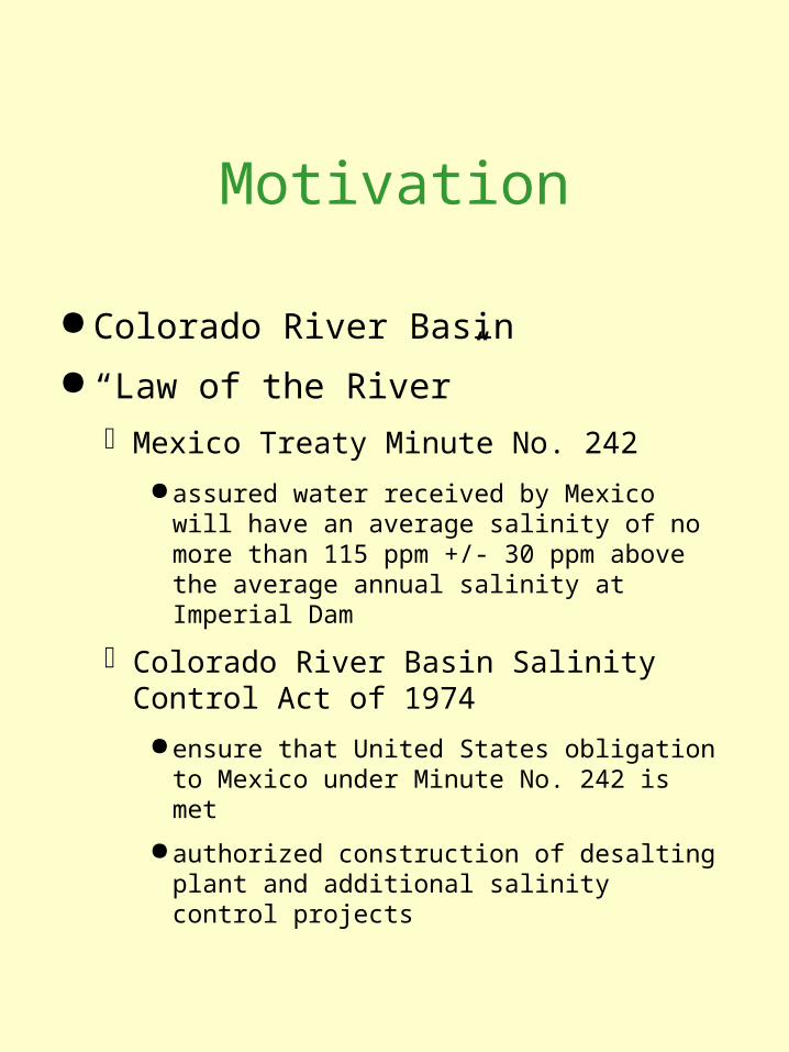
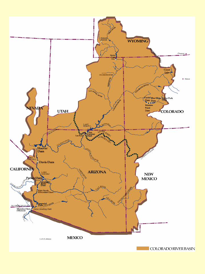
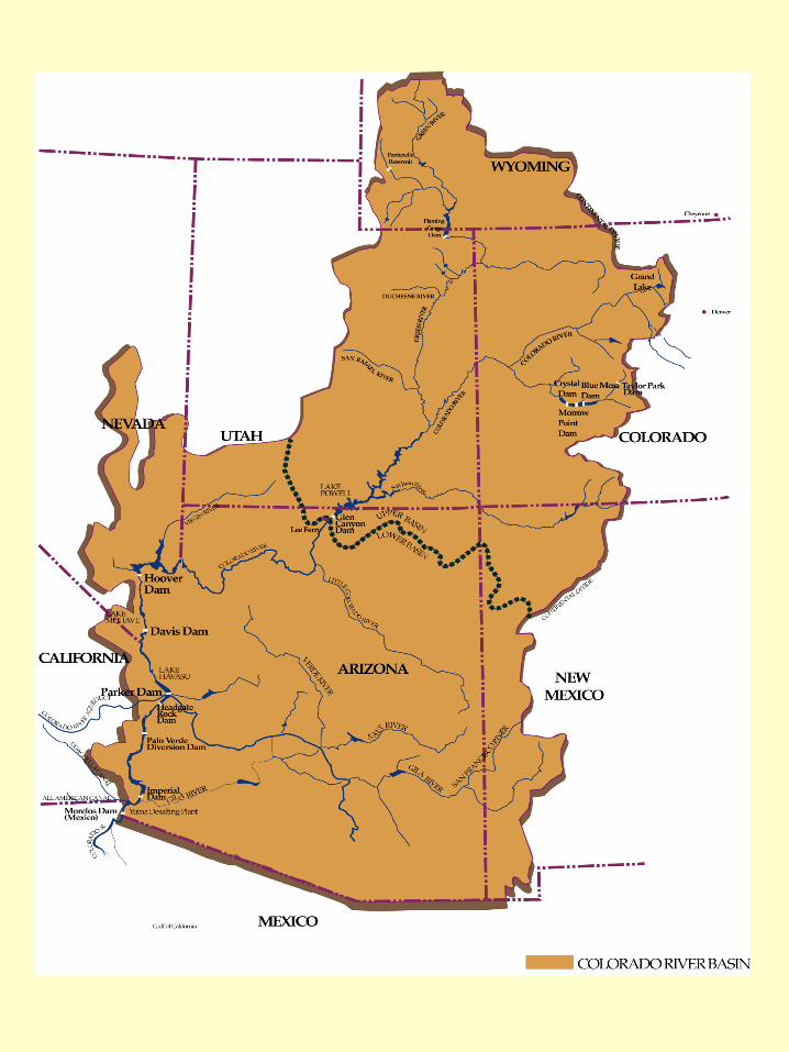
Colorado River Basin

“Law of the River”

Mexico Treaty Minute No. 242

assured water received by Mexico will have an average salinity of no more than 115 ppm +/- 30 ppm above the average annual salinity at Imperial Dam

Colorado River Basin Salinity Control Act of 1974

ensure that United States obligation to Mexico under Minute No. 242 is met

authorized construction of desalting plant and additional salinity control projects

Motivation

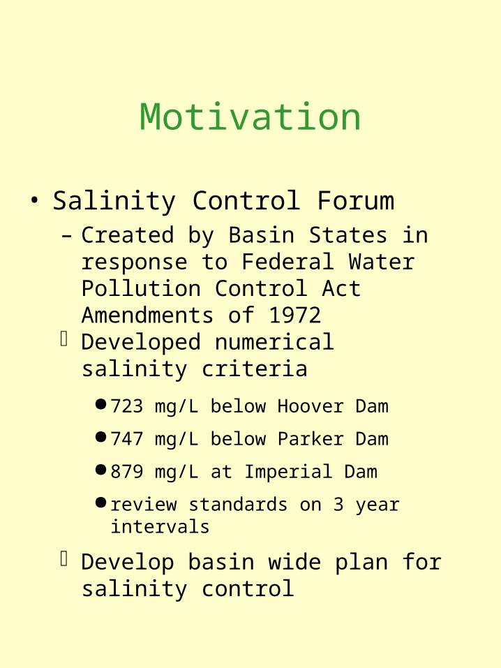
• Salinity Control Forum

– Created by Basin States in response to Federal Water Pollution Control Act Amendments of 1972

Developed numerical salinity criteria

723 mg/L below Hoover Dam

747 mg/L below Parker Dam

879 mg/L at Imperial Dam

review standards on 3 year intervals

Develop basin wide plan for salinity control

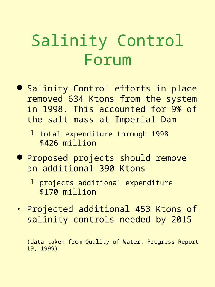
Salinity Control Forum

Salinity Control efforts in place removed 634 Ktons from the system in 1998. This accounted for 9% of the salt mass at Imperial Dam

total expenditure through 1998 $426 million

Proposed projects should remove an additional 390 Ktons

projects additional expenditure $170 million

• Projected additional 453 Ktons of salinity controls needed by 2015

(data taken from Quality of Water, Progress Report 19, 1999)

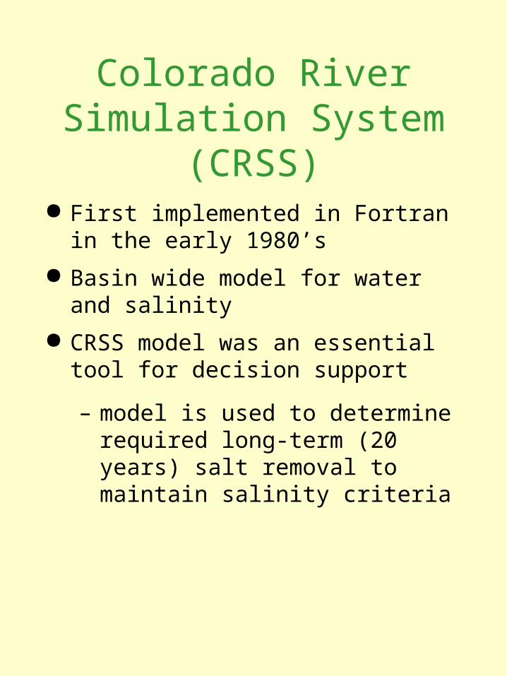
Colorado River Simulation System (CRSS)

First implemented in Fortran in the early 1980’s

Basin wide model for water and salinity

CRSS model was an essential tool for decision support

– model is used to determine required long-term (20 years) salt removal to maintain salinity criteria

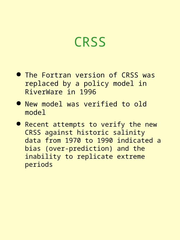
CRSS

The Fortran version of CRSS was replaced by a policy model in RiverWare in 1996

New model was verified to old model

Recent attempts to verify the new CRSS against historic salinity data from 1970 to 1990 indicated a bias (over-prediction) and the inability to replicate extreme periods

CRSS

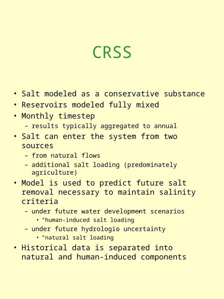
• Salt modeled as a conservative substance• Reservoirs modeled fully mixed• Monthly timestep

– results typically aggregated to annual

• Salt can enter the system from two sources– from natural flows

– additional salt loading (predominately agriculture)

• Model is used to predict future salt removal necessary to maintain salinity criteria– under future water development scenarios

• “human-induced salt loading”

– under future hydrologic uncertainty• “natural salt loading”

• Historical data is separated into natural and human-induced components

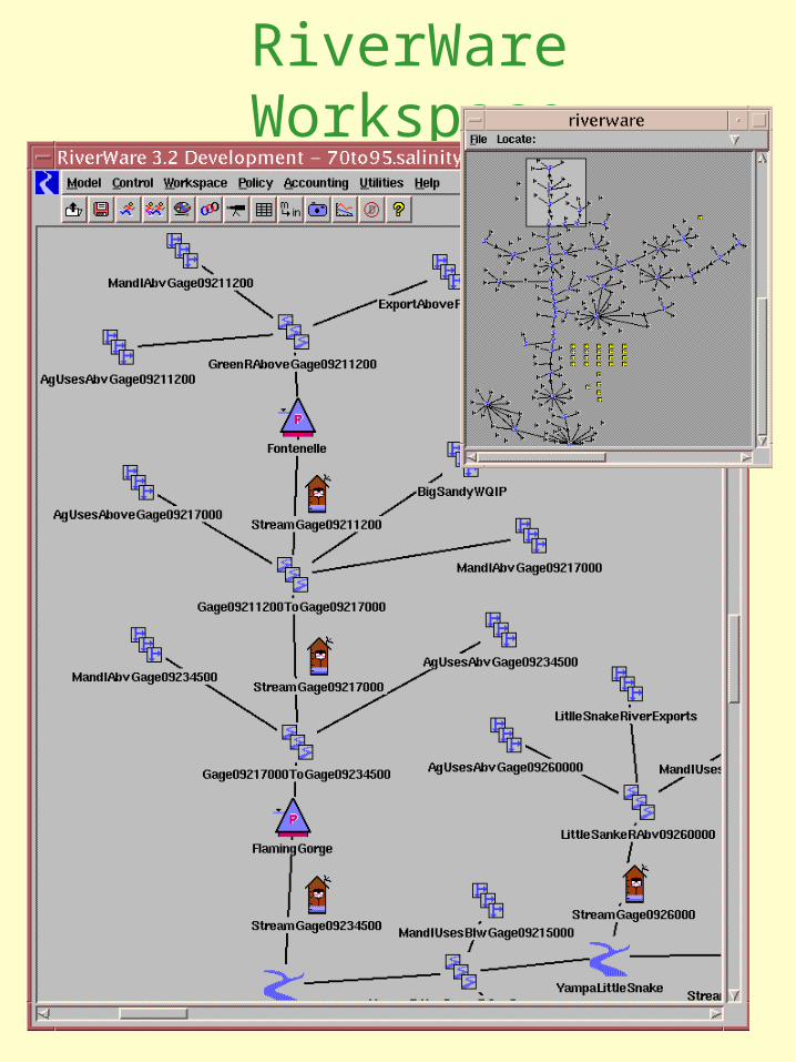
RiverWare Workspace

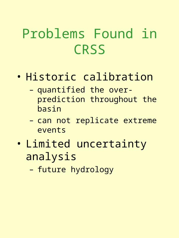
Problems Found in CRSS

• Historic calibration– quantified the over-prediction

throughout the basin

– can not replicate extreme events

• Limited uncertainty analysis– future hydrology

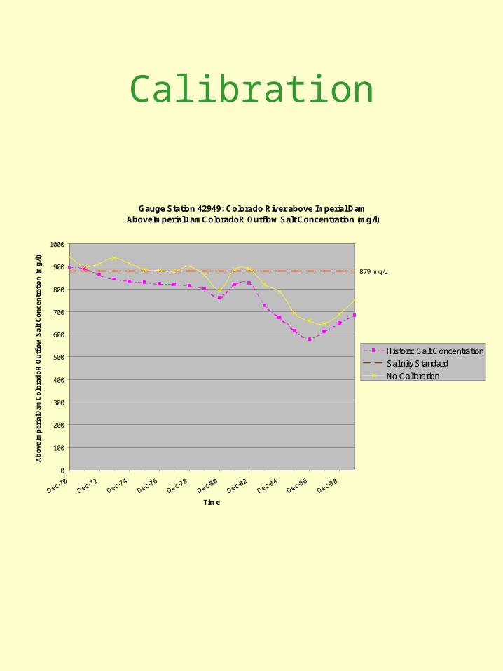
Gauge Station 42949: Colorado River above Imperial Dam AboveImperialDamColoradoR Outflow Salt Concentration (mg/l)

0

100

200

300

400

500

600

700

800

900

1000

Dec-70

Dec-72

Dec-74

Dec-76

Dec-78

Dec-80

Dec-82

Dec-84

Dec-86

Dec-88

Time

Ab

ove

Imp

eria

lDam

Co

lora

do

R O

utf

low

Sal

t C

on

cen

trat

ion

(m

g/l

)

Historic Salt Concentration

Salinity Standard

No Calibration

879 mg/L

Calibration

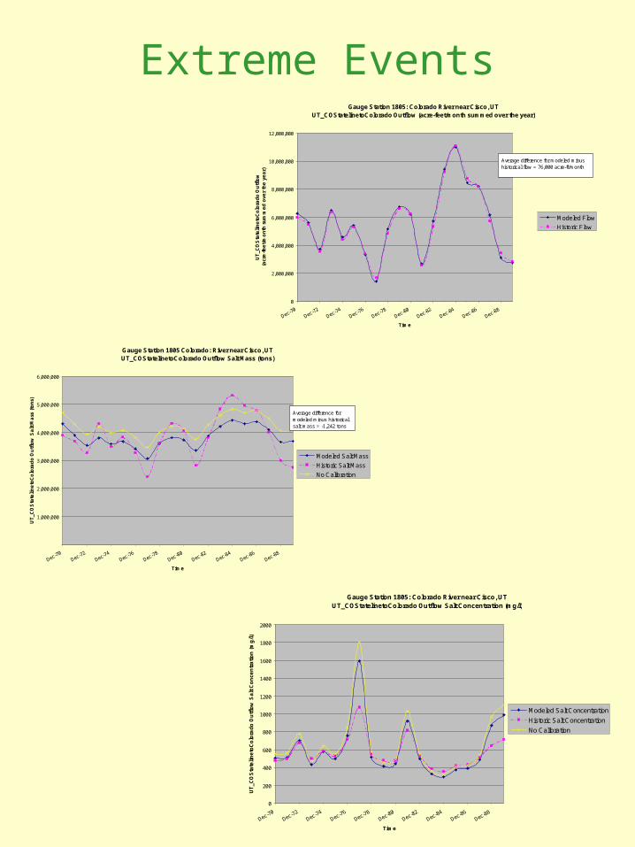
Gauge Station 1805: Colorado River near Cisco, UTUT_COStatelinetoColorado Outflow (acre-feet/month summed over the year)

0

2,000,000

4,000,000

6,000,000

8,000,000

10,000,000

12,000,000

Dec-70Dec-72

Dec-74Dec-76

Dec-78Dec-80

Dec-82Dec-84

Dec-86Dec-88

Time

UT

_CO

Sta

teli

ne

toC

olo

rad

o O

utf

low

(a

cre

-fe

et/

mo

nth

su

mm

ed

ove

r th

e y

ea

r)

Modeled Flow

Historic Flow

Average difference for modeled minus historical flow = 76,000 acre-ft/month

Extreme Events

Gauge Station 1805: Colorado River near Cisco, UTUT_COStatelinetoColorado Outflow Salt Concentration (mg/l)

0

200

400

600

800

1000

1200

1400

1600

1800

2000

Dec-70Dec-72

Dec-74Dec-76

Dec-78Dec-80

Dec-82Dec-84

Dec-86Dec-88

Time

UT

_CO

Sta

teli

ne

toC

olo

rad

o O

utf

low

Sa

lt C

on

cen

tra

tio

n (

mg

/l)

Modeled Salt Concentration

Historic Salt Concentration

No Calibration

Gauge Station 1805 Colorado: River near Cisco, UTUT_COStatelinetoColorado Outflow Salt Mass (tons)

1,000,000

2,000,000

3,000,000

4,000,000

5,000,000

6,000,000

Dec-70Dec-72

Dec-74Dec-76

Dec-78Dec-80

Dec-82Dec-84

Dec-86Dec-88

Time

UT

_CO

Sta

teli

ne

toC

olo

rad

o O

utf

low

Sa

lt M

ass

(to

ns)

Modeled Salt Mass

Historic Salt Mass

No Calibration

Average difference for modeled minus historical salt mass = -1,242 tons

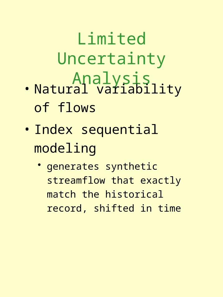
Limited Uncertainty Analysis

• Natural variability of flows

• Index sequential modeling generates synthetic streamflow that

exactly match the historical record,

shifted in time

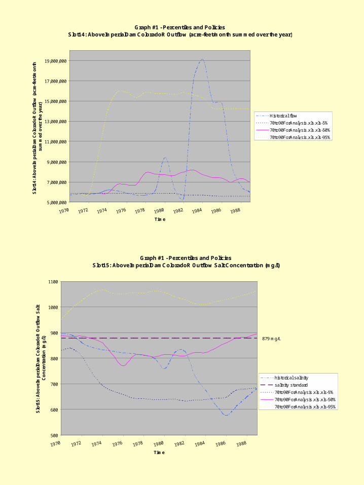
Graph #1 - Percentiles and PoliciesSlot14: AboveImperialDamColoradoR Outflow (acre-feet/month summed over the year)

5,000,000

7,000,000

9,000,000

11,000,000

13,000,000

15,000,000

17,000,000

19,000,000

1970 1972 1974 1976 1978 1980 1982 1984 1986 1988

Time

Slo

t14:

Ab

ove

Imp

eria

lDam

Co

lora

do

R O

utf

low

(ac

re-f

eet/

mo

nth

su

mm

ed o

ver

the

year

)

Historical flow

70to90ForAnalysis.xls.xls-5%



Graph #1 - Percentiles and PoliciesSlot15: AboveImperialDamColoradoR Outflow Salt Concentration (mg/l)

500

600

700

800

900

1000

1100

1970 1972 1974 1976 1978 1980 1982 1984 1986 1988

Time

Slo

t15:

Ab

ove

Imp

eria

lDam

Co

lora

do

R O

utf

low

Sal

t C

on

cen

trat

ion

(m

g/l

)

historical salinity

salinity standard




879 mg/L

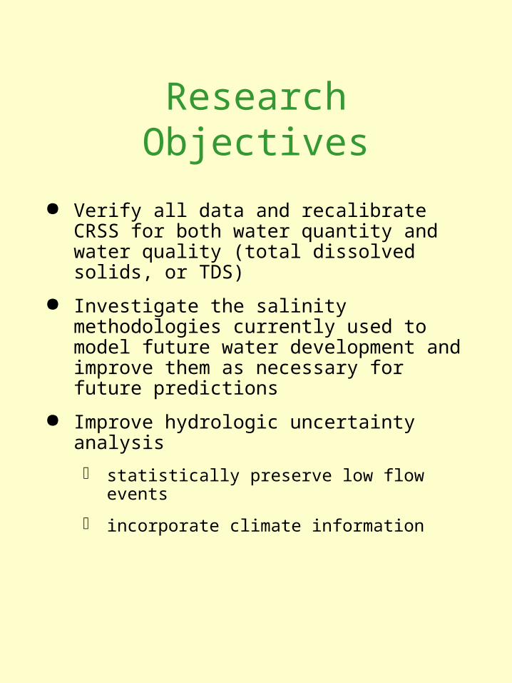
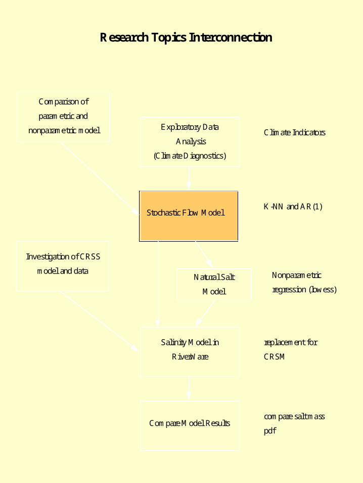
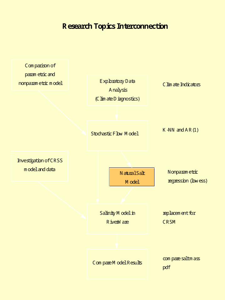
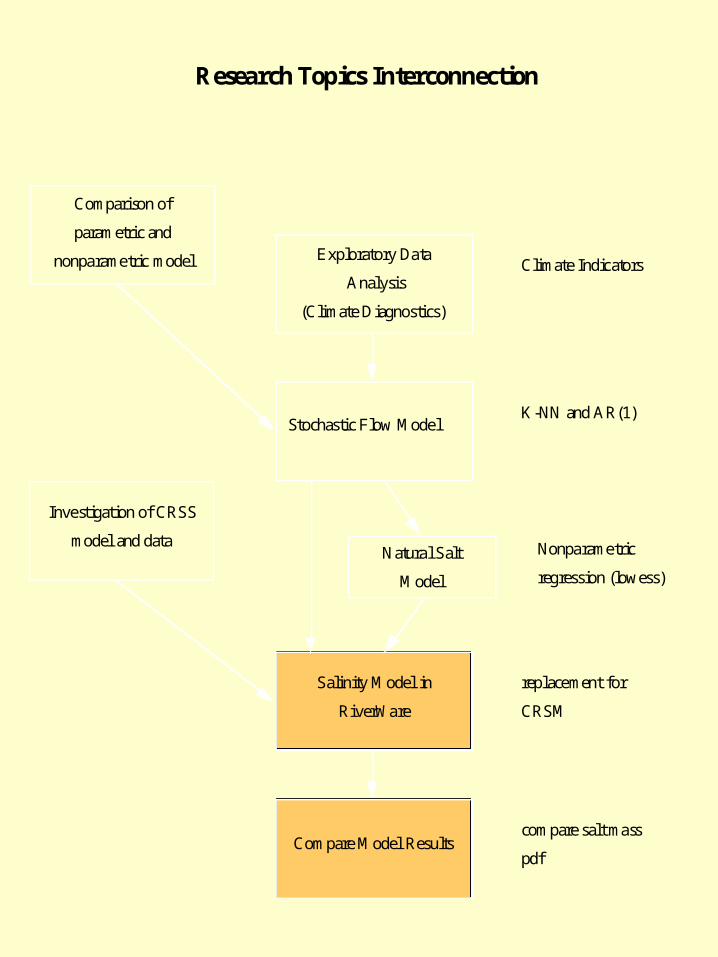
Research Objectives

Verify all data and recalibrate CRSS for both water quantity and water quality (total dissolved solids, or TDS)

Investigate the salinity methodologies currently used to model future water development and improve them as necessary for future predictions

Improve hydrologic uncertainty analysis

statistically preserve low flow events

incorporate climate information

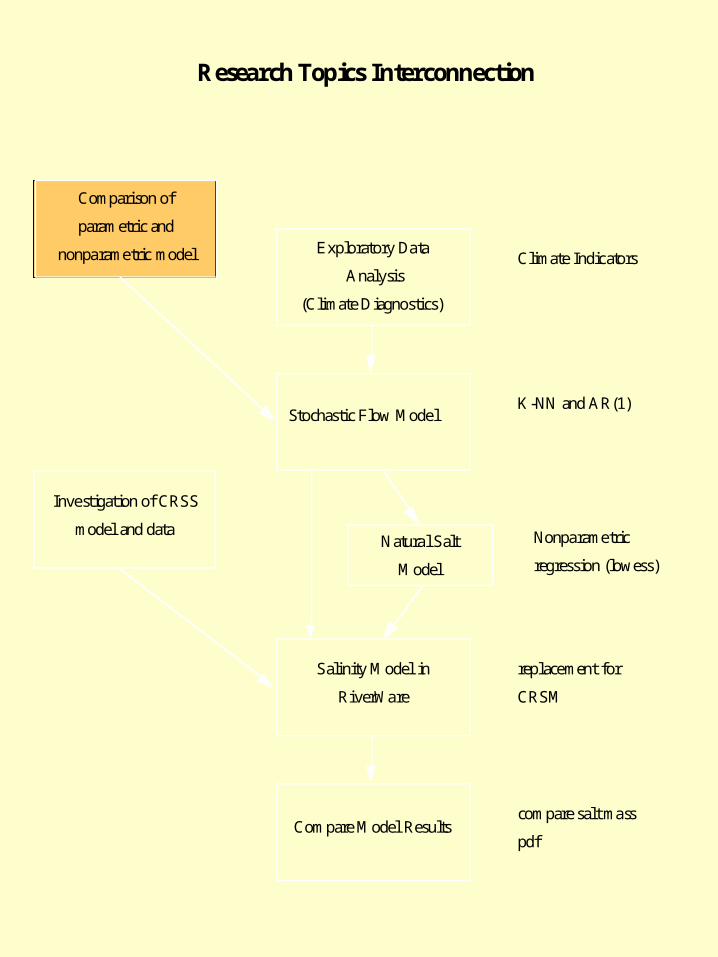
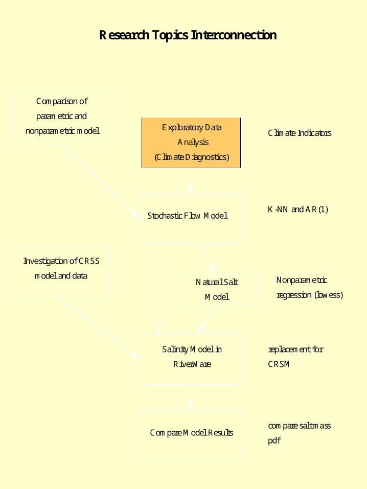
Exploratory Data

Analysis

(Climate Diagnostics)

Stochastic Flow Model

Salinity Model in

RiverWare

Compare Model Results

Comparison of

parametric and

nonparametric model

Natural Salt

Model

Climate Indicators

K-NN and AR(1)

Nonparametric

regression (lowess)

replacement for

CRSM

compare salt mass

pdf

Research Topics Interconnection

Investigation of CRSS

model and data

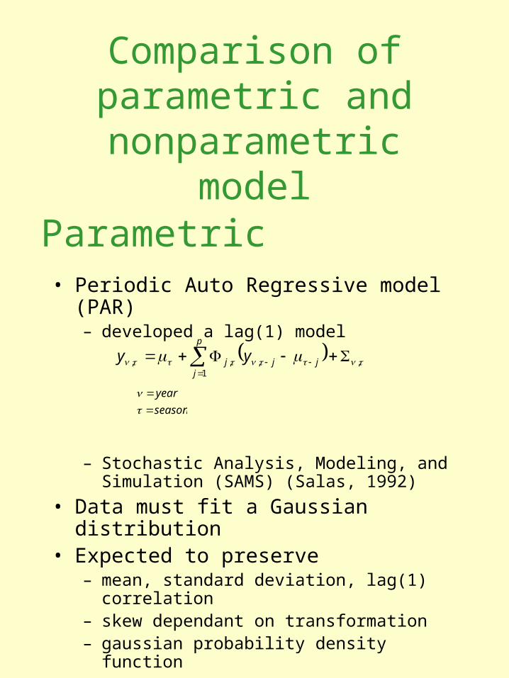
Parametric• Periodic Auto Regressive model (PAR)

– developed a lag(1) model

– Stochastic Analysis, Modeling, and Simulation (SAMS) (Salas, 1992)

• Data must fit a Gaussian distribution• Expected to preserve

– mean, standard deviation, lag(1) correlation– skew dependant on transformation– gaussian probability density function

( )å=

-- S+-F+=p

jjjj yy

1,,,, tnttntttn mm

season

year

==

tn

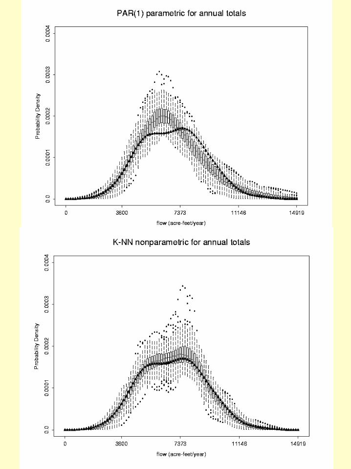
Comparison of parametric and nonparametric model

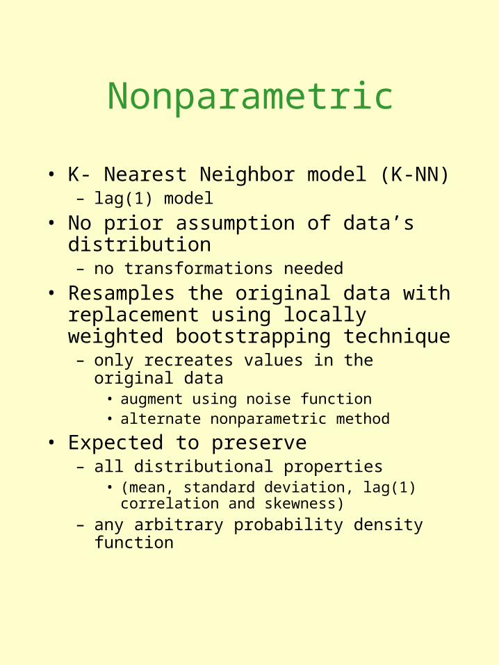
Nonparametric

• K- Nearest Neighbor model (K-NN)– lag(1) model

• No prior assumption of data’s distribution– no transformations needed

• Resamples the original data with replacement using locally weighted bootstrapping technique– only recreates values in the original data

• augment using noise function• alternate nonparametric method

• Expected to preserve– all distributional properties

• (mean, standard deviation, lag(1) correlation and skewness)

– any arbitrary probability density function

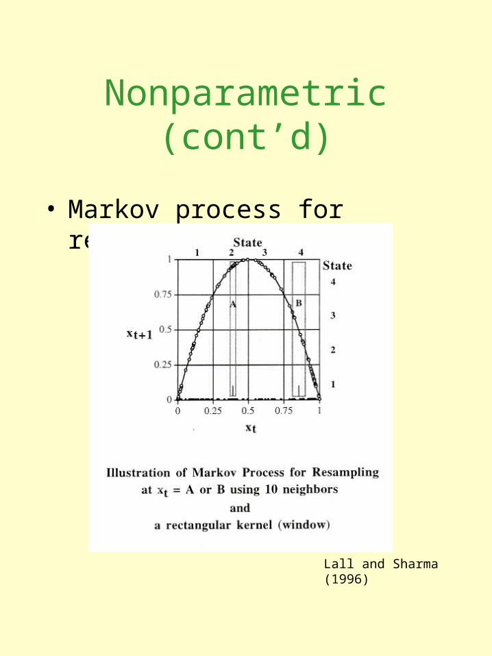
Nonparametric (cont’d)

• Markov process for resampling

Lall and Sharma (1996)

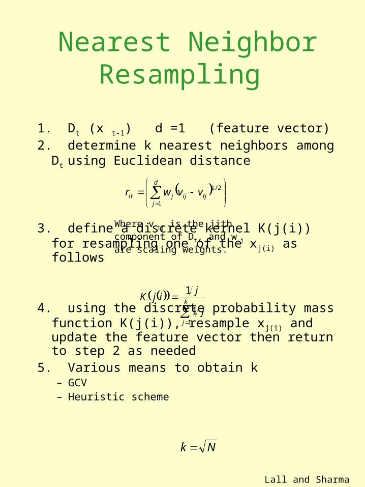
Nearest Neighbor Resampling

1. Dt (x t-1) d =1 (feature vector)

2. determine k nearest neighbors among Dt using Euclidean distance

3. define a discrete kernel K(j(i)) for resampling one of the xj(i) as follows

4. using the discrete probability mass function K(j(i)), resample xj(i) and update the feature vector then return to step 2 as needed

5. Various means to obtain k– GCV– Heuristic scheme

( ) ÷÷ø

öççè

æ-= å

=

d

jtjijjit vvwr

1

2/1

Where v tj is the jith component of Dt, and w j are scaling weights.

( )( )å

=

=k

j

j

jijK

1

1

1

Lall and Sharma (1996)

Nk =

Annual Water Year Natural FlowUSGS stream gauge 09180500 (Colorado River near Cisco, UT)

0

2000

4000

6000

8000

10000

12000

14000

1906

1909

1912

1915

1918

1921

1924

1927

1930

1933

1936

1939

1942

1945

1948

1951

1954

1957

1960

1963

1966

1969

1972

1975

1978

1981

1984

1987

1990

flo

w (

1000

acr

e-fe

et/y

ear)

Monthly Natural FlowUSGS stream gauge 09180500 (Colorado River near Cisco, UT)

0

500

1000

1500

2000

2500

3000

3500

4000

Oct-05

Oct-08

Oct-11

Oct-14

Oct-17

Oct-20

Oct-23

Oct-26

Oct-29

Oct-32

Oct-35

Oct-38

Oct-41

Oct-44

Oct-47

Oct-50

Oct-53

Oct-56

Oct-59

Oct-62

Oct-65

Oct-68

Oct-71

Oct-74

Oct-77

Oct-80

Oct-83

Oct-86

Oct-89

flo

w (

1000

acr

e-fe

et/m

on

th)

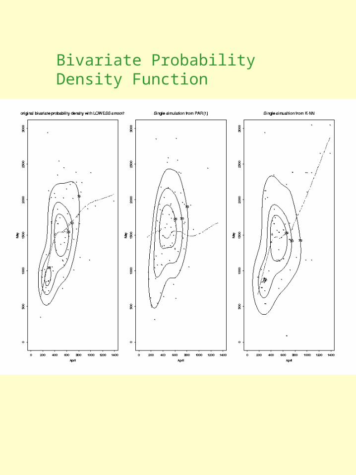
Bivariate Probability Density Function

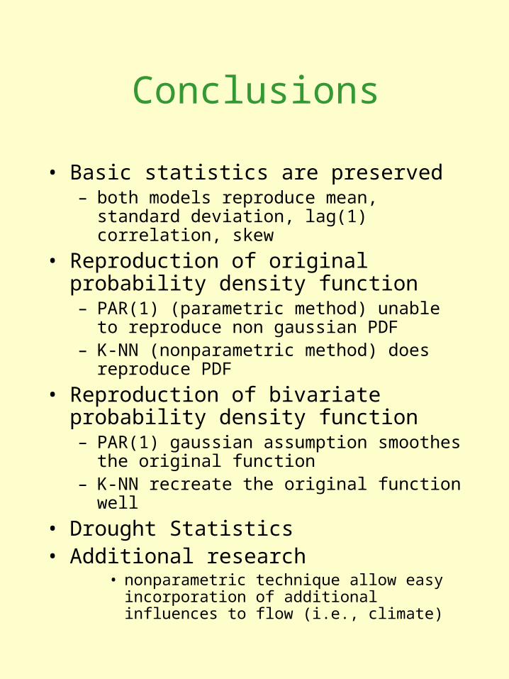
Conclusions

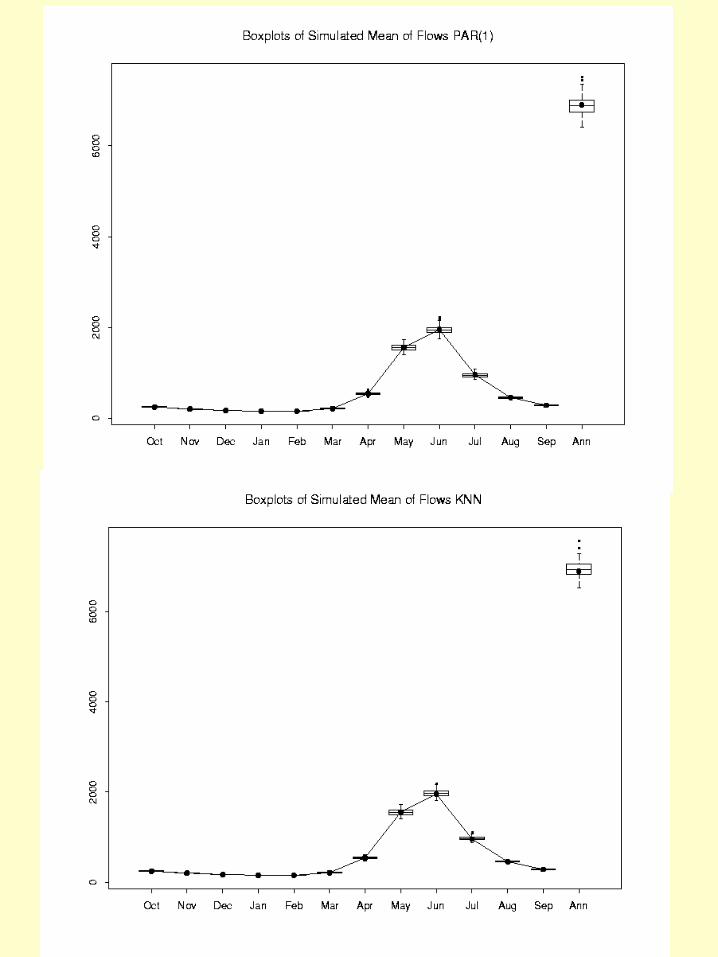
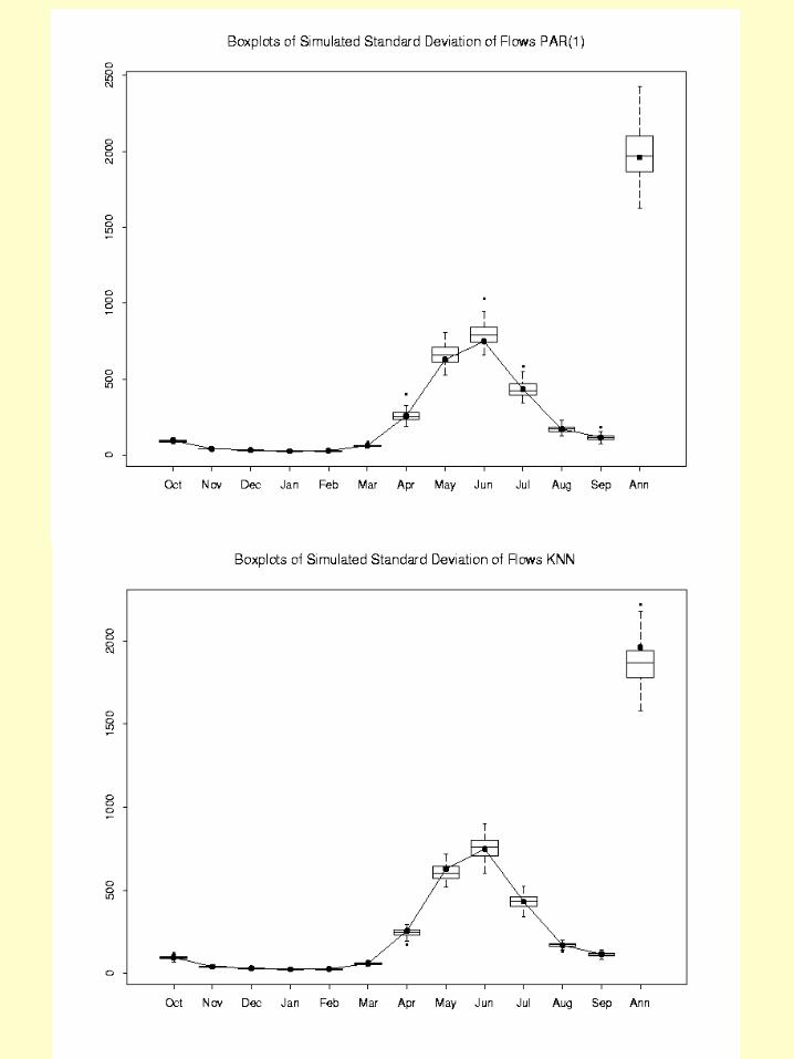
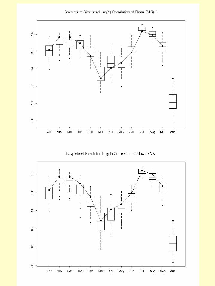
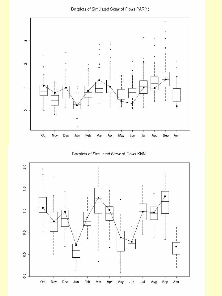
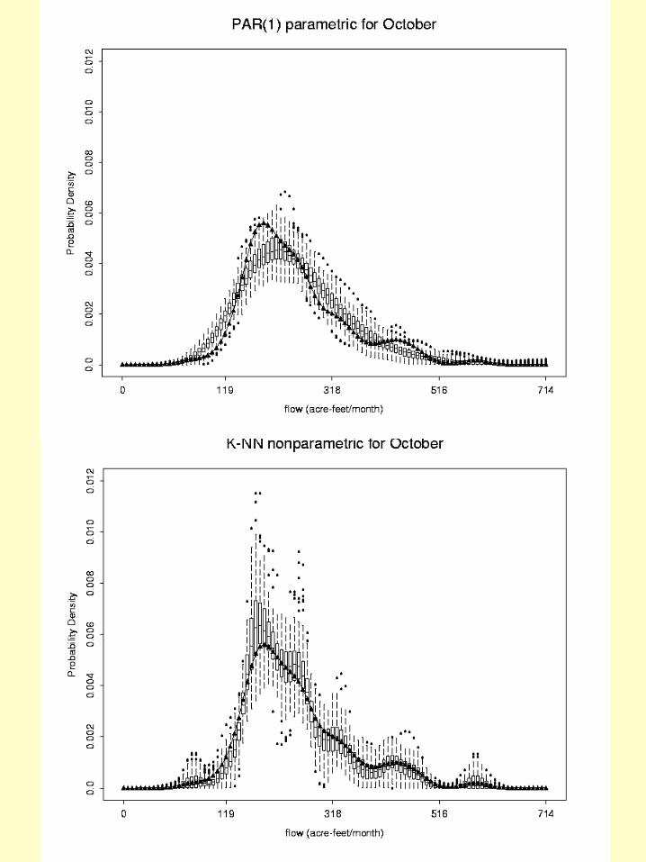
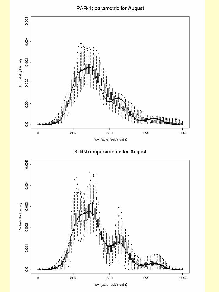
• Basic statistics are preserved– both models reproduce mean, standard

deviation, lag(1) correlation, skew

• Reproduction of original probability density function– PAR(1) (parametric method) unable to

reproduce non gaussian PDF – K-NN (nonparametric method) does reproduce

PDF

• Reproduction of bivariate probability density function– PAR(1) gaussian assumption smoothes the

original function– K-NN recreate the original function well

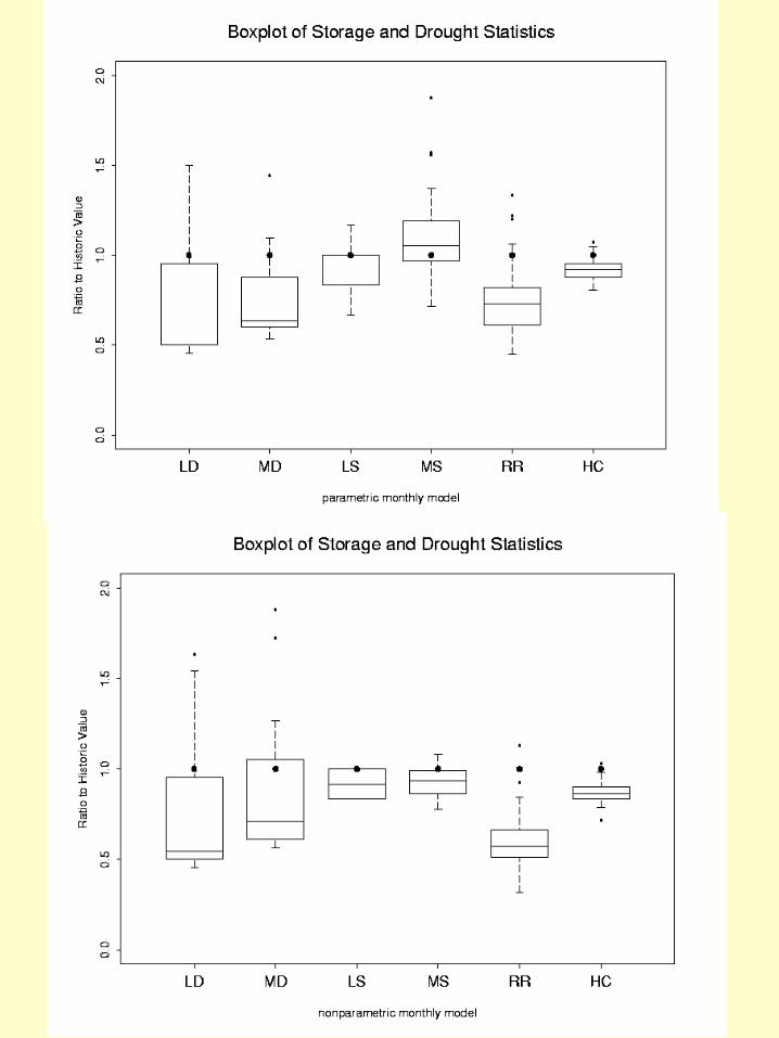
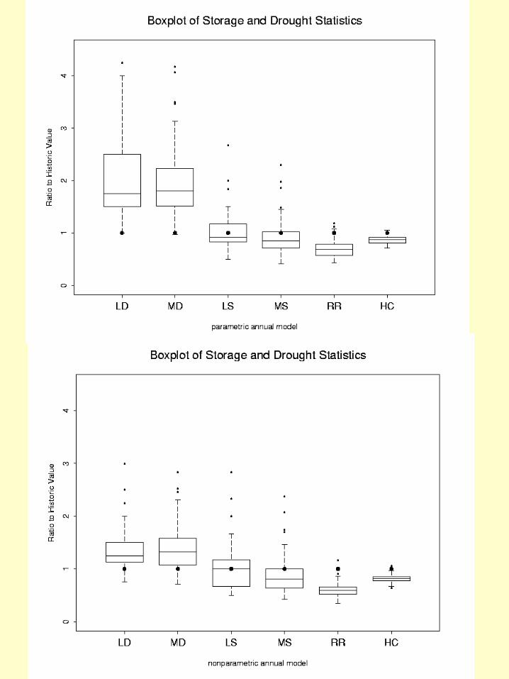
• Drought Statistics• Additional research

• nonparametric technique allow easy incorporation of additional influences to flow (i.e., climate)

Exploratory Data

Analysis



Salinity Model in

RiverWare


Comparison of

parametric and

nonparametric model

Natural Salt

Model

Climate Indicators

K-NN and AR(1)

Nonparametric

regression (lowess)

replacement for

CRSM

compare salt mass

pdf



model and data

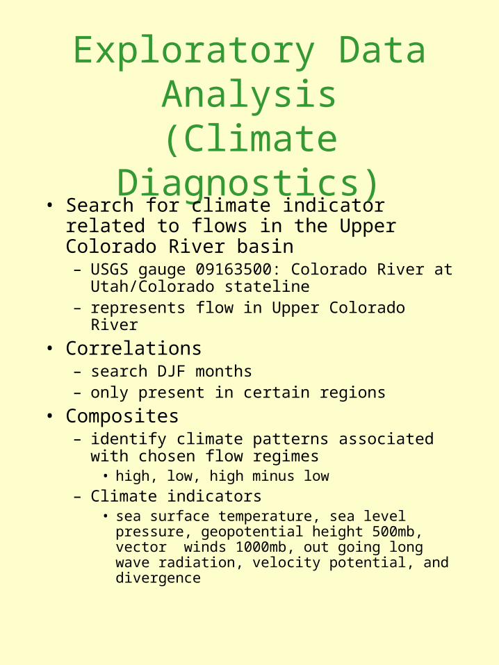
Exploratory Data Analysis(Climate Diagnostics)

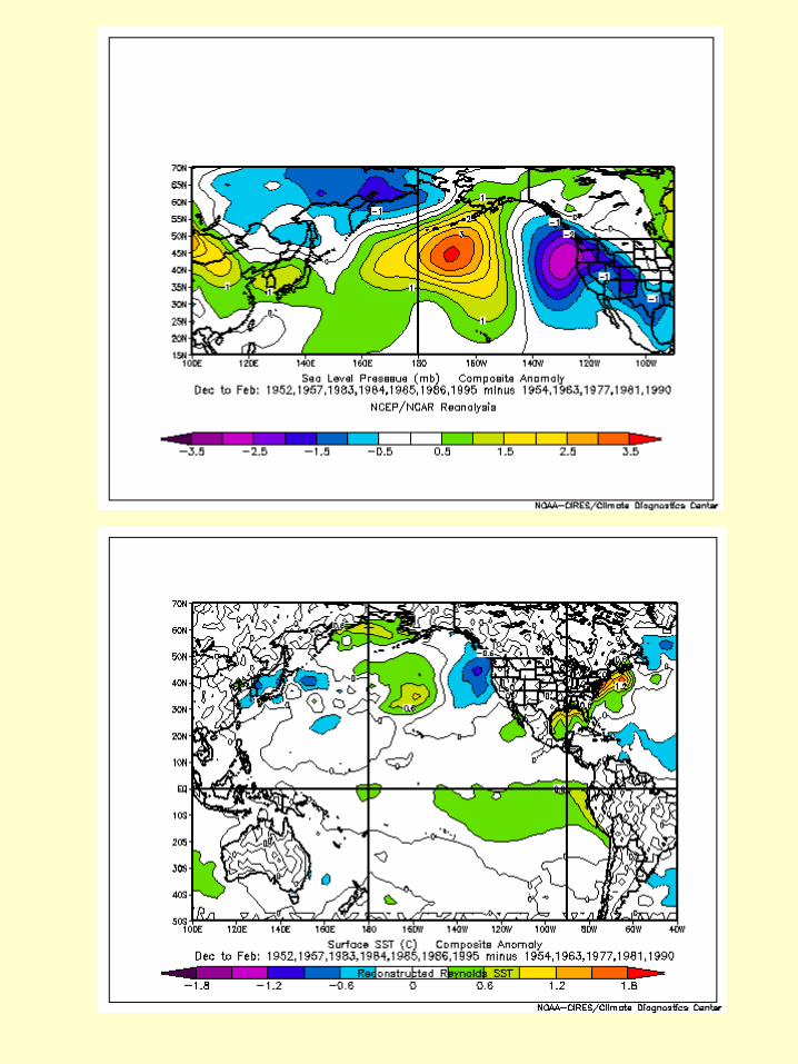
• Search for climate indicator related to flows in the Upper Colorado River basin– USGS gauge 09163500: Colorado River at

Utah/Colorado stateline– represents flow in Upper Colorado River

• Correlations– search DJF months– only present in certain regions

• Composites– identify climate patterns associated with chosen

flow regimes• high, low, high minus low

– Climate indicators• sea surface temperature, sea level pressure,

geopotential height 500mb, vector winds 1000mb, out going long wave radiation, velocity potential, and divergence

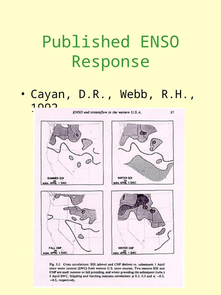
Published ENSO Response

• Cayan, D.R., Webb, R.H., 1992.

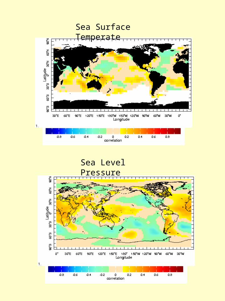
Sea Surface Temperate

Sea Level Pressure

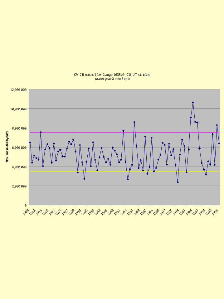
CWCB natural flow Gauge 1635: @ CO-UT stateline(water year Oct to Sept)

0

2,000,000

4,000,000

6,000,000

8,000,000

10,000,000

12,000,000

1909

1912

1915

1918

1921

1924

1927

1930

1933

1936

1939

1942

1945

1948

1951

1954

1957

1960

1963

1966

1969

1972

1975

1978

1981

1984

1987

1990

1993

1996

flo

w (

acre

-fee

t/ye

ar)

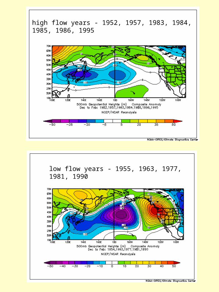
high flow years - 1952, 1957, 1983, 1984, 1985, 1986, 1995

low flow years - 1955, 1963, 1977, 1981, 1990

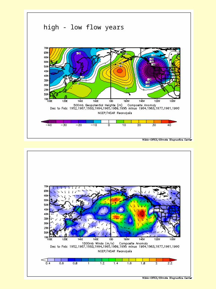
high - low flow years

Conclusions

• Found unique climate patterns for high and low flows

• High minus low displayed a difference for each flow regime– geopotential height at 500mb showed the

strongest signal

– climate signal similar to ENSO• influence by ENSO through teleconnections

• Time series analysis of Geopotential Height at 500mb– principal component analysis

• PC(1) structure

– develop relationship for flow dependant on climate

Exploratory Data

Analysis



Salinity Model in

RiverWare


Comparison of

parametric and

nonparametric model

Natural Salt

Model

Climate Indicators

K-NN and AR(1)

Nonparametric

regression (lowess)

replacement for

CRSM

compare salt mass

pdf



model and data


• Natural flows will be determined from a multiple step process– nonparametric smooth bootstrap method to

develop an index of PC(1)– the k-nearest neighbor method uses locally

weighted resamples of the PC(1) for the current year to be simulated based on the index of PC(1) for the previous year

– the annual flow associated with the simulated PC(1) becomes the annual flow for the current year simulated

• Hypothesis:– Conditioning the nonparametric model on large

scale climate will improve the stochastic modeling of extreme events

• probability of extreme events

• Annual timestep

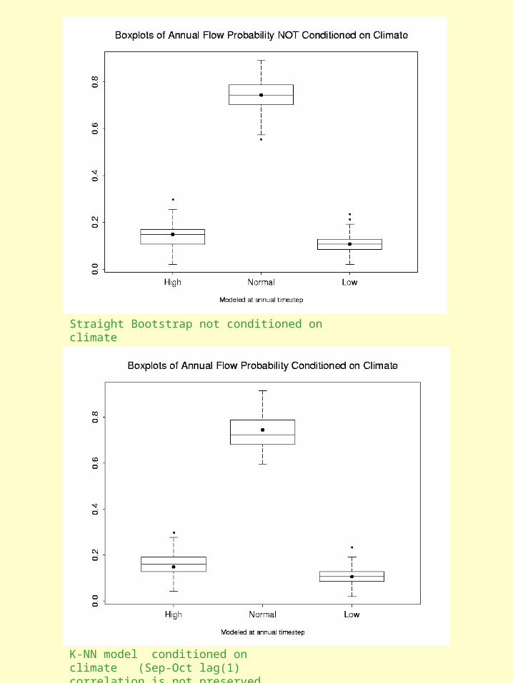
Straight Bootstrap not conditioned on climate

K-NN model conditioned on climate (Sep-Oct lag(1) correlation is not preserved

Exploratory Data

Analysis



Salinity Model in

RiverWare


Comparison of

parametric and

nonparametric model

Natural Salt

Model

Climate Indicators

K-NN and AR(1)

Nonparametric

regression (lowess)

replacement for

CRSM

compare salt mass

pdf



model and data

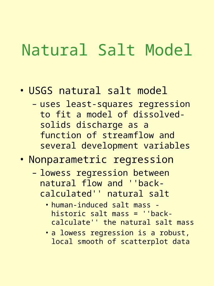
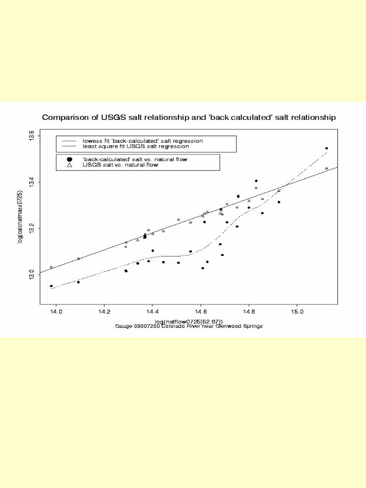
Natural Salt Model

• USGS natural salt model– uses least-squares regression to fit a

model of dissolved-solids discharge as a function of streamflow and several development variables

• Nonparametric regression– lowess regression between natural flow

and ''back-calculated'' natural salt • human-induced salt mass - historic salt

mass = ''back-calculate'' the natural salt mass

• a lowess regression is a robust, local smooth of scatterplot data

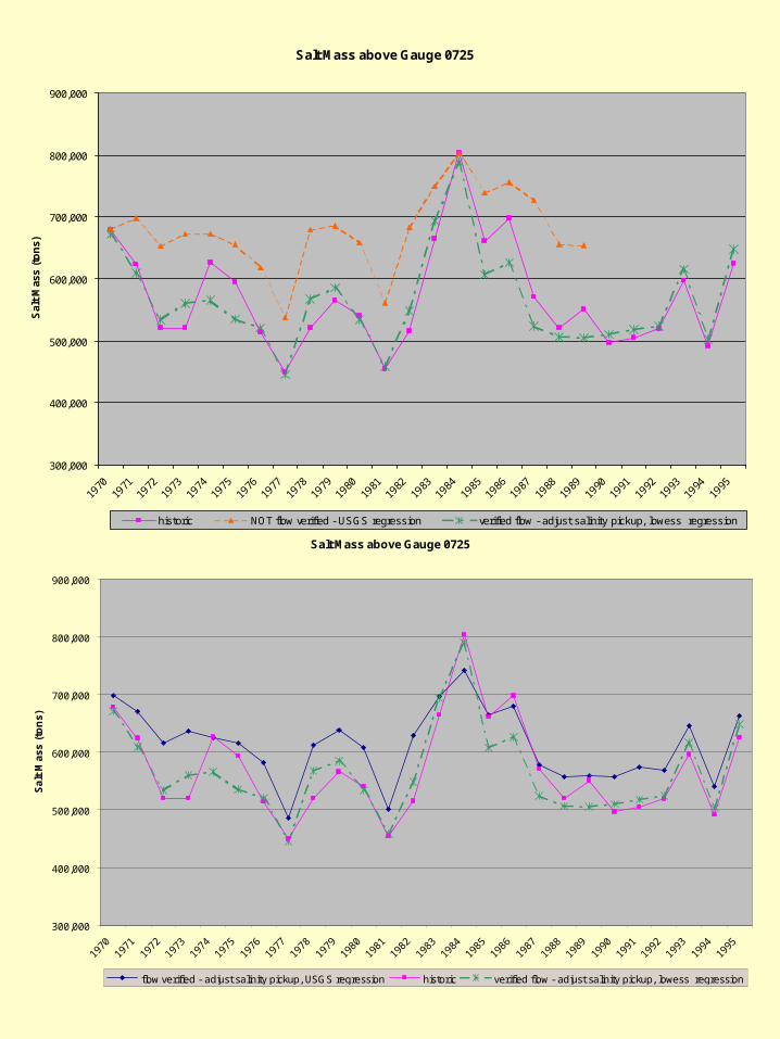
Salt Mass above Gauge 0725

300,000

400,000

500,000

600,000

700,000

800,000

900,000

1970

1971

1972

1973

1974

1975

1976

1977

1978

1979

1980

1981

1982

1983

1984

1985

1986

1987

1988

1989

1990

1991

1992

1993

1994

1995

Sa

lt M

as

s (

ton

s)

flow verified - adjust salinity pickup, USGS regression historic verified flow - adjust salinity pickup, lowess regression

Salt Mass above Gauge 0725

300,000

400,000

500,000

600,000

700,000

800,000

900,000

1970

1971

1972

1973

1974

1975

1976

1977

1978

1979

1980

1981

1982

1983

1984

1985

1986

1987

1988

1989

1990

1991

1992

1993

1994

1995

Sal

t M

ass

(to

ns)

historic NOT flow verified - USGS regression verified flow - adjust salinity pickup, lowess regression

Exploratory Data

Analysis



Salinity Model in

RiverWare


Comparison of

parametric and

nonparametric model

Natural Salt

Model

Climate Indicators

K-NN and AR(1)

Nonparametric

regression (lowess)

replacement for

CRSM

compare salt mass

pdf



model and data

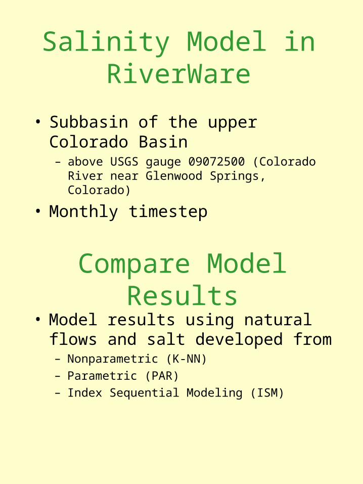
Salinity Model in RiverWare

• Subbasin of the upper Colorado Basin – above USGS gauge 09072500 (Colorado River

near Glenwood Springs, Colorado)

• Monthly timestep


• Model results using natural flows and salt developed from– Nonparametric (K-NN)

– Parametric (PAR)

– Index Sequential Modeling (ISM)

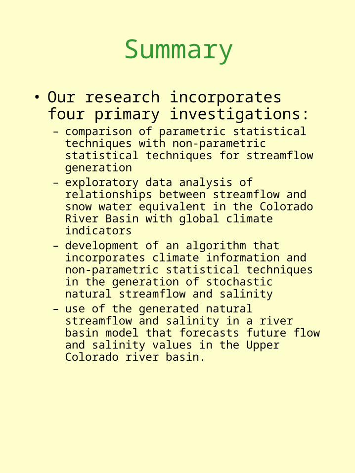
Summary

• Our research incorporates four primary investigations:– comparison of parametric statistical techniques

with non-parametric statistical techniques for streamflow generation

– exploratory data analysis of relationships between streamflow and snow water equivalent in the Colorado River Basin with global climate indicators

– development of an algorithm that incorporates climate information and non-parametric statistical techniques in the generation of stochastic natural streamflow and salinity

– use of the generated natural streamflow and salinity in a river basin model that forecasts future flow and salinity values in the Upper Colorado river basin.

Documents

Incorporating Climate Information in Long Term Salinity Prediction with Uncertainty Analysis James Prairie(1,2), Balaji Rajagopalan(1), and Terry Fulp(2)