Income and Happiness - NIU College of Educationcedu.niu.edu/~walker/statistics/K-12 Simple Linear Regression.pdf · The research study employed simple linear regression analysis to

INCOME AND HAPPINESS 1

Income and Happiness

Abstract

Are wealthier people happier? The research study employed simple linear regression analysis to

confirm the positive relationship between income and happiness. The study obtained data from

an existing dataset by selecting only 959 participants in New York City. The results indicated that

there is a statistically significant positive relationship between income and happiness; however,

the relationship is really weak, which is consistent with the previous research studies. Thus, the

answer to the research question is “yes” people who have more money are happier than those

who have less. As income is slightly related to happiness, future research should extensively

focus on more independent variables in the study such as age, health, education and employment.


Introduction

Are wealthier people happier? This question has been widely asked among economists

and socialists in this contemporary society. In general, people firmly believe that if they have

more money, their life would be much better. Based on conventional economics, it is believed

that money can buy happiness. It is because money can be used to exchange for things to satisfy

people’s needs. Likewise, a research study conducted by Schnittker (2008) found that the

correlation between income and happiness is always understood in terms of income allowing

people to enjoy their life and consume goods to fulfill their needs and increase their well-being.

Therefore, money and happiness are highly linked, and usually it is believed that people with

higher income are happier than people with lower income; in other words, people with lower

income are less happy than people with higher income.

There have been extensive research related to the relationship between income and

happiness. Most of the evidence indicates that there is a positive relationship between income

and happiness (Schnittker, 2008). Higher incomes and greater happiness are highly linked.

Schnittker (2008) believed that this positive relationship is not surprising, and people usually use

socio-economic status as a key element to explain characteristics of quality of life. Based on

Diener (1984) Wealthy people would describe their life as good, and tend to satisfy with their life

much better than less wealthy people within a given society (as cited in Boyce, Brown, & Moore,

2010).

Therefore, the purpose of this research study is to confirm the positive bivariate

relationship between income and happiness. In other words, it is to confirm if people who have

more money are happier than those who have less money. The study aims to answer the research

question: to what extent is income related to happiness? The null hypothesis (H0) is “There is no


statistically significant relationship between income and happiness”, while the alternative

hypothesis (H1) is “There is a statistically significant relationship between income and

happiness”.

Literature Review

The relationship between income and happiness has been studied by many researchers,

especially economists. According to Hernandez-Murillo (2010), Richard Easterlin was the first

modern economist who investigated the association between income and happiness (as cited in

Como, 2011). Easterlin has done extensive research regarding the income-happiness relationship.

Through his investigations, Easterlin (2001) found three empirical regularities to explain his

theory. Firstly, at a given time people with higher income are happier than those with less

income. Secondly, over the life cycle, the level of happiness remains stable in spite of a growth

in the level of income. Finally, people tend to believe that they were less happy in the past and

happier in the future.

Easterlin (2001) observed the relationship between income and happiness. He found that

in each representative national survey, a statistically significant positive bivariate relationship

between income and happiness has always been found (Andrews, 1986, p. xi; Argyle, 1999, pp.

356-7; Diener, 1984, p.553 as cited in Easterlin, 2001). According to the General Social Survey

(GSS) in the United States in 1994, a direct question regarding subjective well-being was used to

measure happiness: “Taken all together, how would you say things are these days – would you

say that you are very happy, pretty happy, or not too happy? (p. 466)”, and it was found that 16%

of people in the lowest income category and 44% of people in the highest income one reported

very happy (cited in Easterlin 2001). By computing the mean of the happiness rating on the scale

“Very happy (4)”, “Pretty happy (2)”, and “Not to happy (0)”, Easterlin (2001) found that the


average point of happiness varies according to the level income, ranging from a low point of 1.8

to a high point of 2.8. Therefore, even though it has been proved that there is a positive

relationship between income and happiness, the relationship between the two variables is often

weak (Howell & Howell, 2008 cited in Boyce et al, 2010; Easterlin, 2001). This would mean

wealthier people are happier, but not very much than less wealthy people at a point in time.

Easterlin (2001) further explained his second principle based on the life cycle principle.

He stated that previous research’s findings were inconsistent regarding the age-happiness

relationship. A study conducted by Mroczek and Kolarz (1998) found a positive relationship

between age and happiness, whereas Myers (1992) found no correlation at all (cited in Easterlin,

2001). A survey conducted by George (1992) found that prior to 1970s older people in the United

States were less happy than younger people, while the recent research studies found differently

that older generation is happier than younger generation (cited in Easterlin, 2001). Easterlin

(2001) explained that such inconsistency caused by the failure to take into account the

plausibility of variation in the relationship over time. According to Easterlin (2001), stability of

happiness in life cycle does not mean that the level of subjective well-being remains constant

over the life time. McLanahan and Sorensen (1985), and Myers (1992) stated that significant

changes of particular circumstances in life cycle such as unemployment, retirement, and death of

family members affect subjective well-being of people (cited in Easterlin, 2001).

Easterlin (2001) continued to explain the last empirical regularity which is the past and

prospective happiness. Based on the observation of life cycle happiness, there is a little change

between people’s past and prospective happiness (Easterlin, 2001). In every survey, participants,

however, generally think at any particular point in the life cycle they are happier today than in

the past, and they will be happier in the future than today (Easterlin, 2001). The periods between


past, today and future are long intervals such as 5 years or more. However, based on Easterlin

(2001), in fact, on average the level of present happiness remains constant. Level of happiness

does not change within a given period of time, but it is people who think they are becoming

happier and happier from present time to the future.

Methods

Data collection

The data for this proposed study were obtained from an empirical study on Inter-

university Consortium for Political and Social Research (ICPSR) website. The method of data

collection was computer-assisted telephone interview (CATI). The data collection date was from

May to November 2006. The original researcher, Lee (2006) conducted the survey on Assessing

happiness and competitiveness of world major metropolises in ten major cities: Beijing, Berlin,

London, Milan, New York city, Paris, Seoul, Stockholm, Tokyo, and Toronto. However, this

proposed study selected only participants in New York City.

Participants

Participants were selected by using representative random sampling method. The

participants were 18 years old and over living in New York City. There were 959 participants in

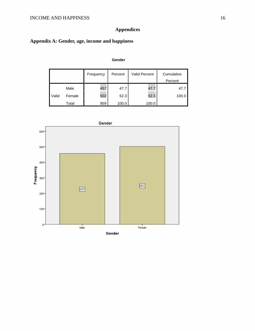
the study. The descriptive statistics showed that there were 457 females and 502 males which

were equal to 47.7% and 52.3% respectively (see Appendix A). Participants’ ages ranged from 18

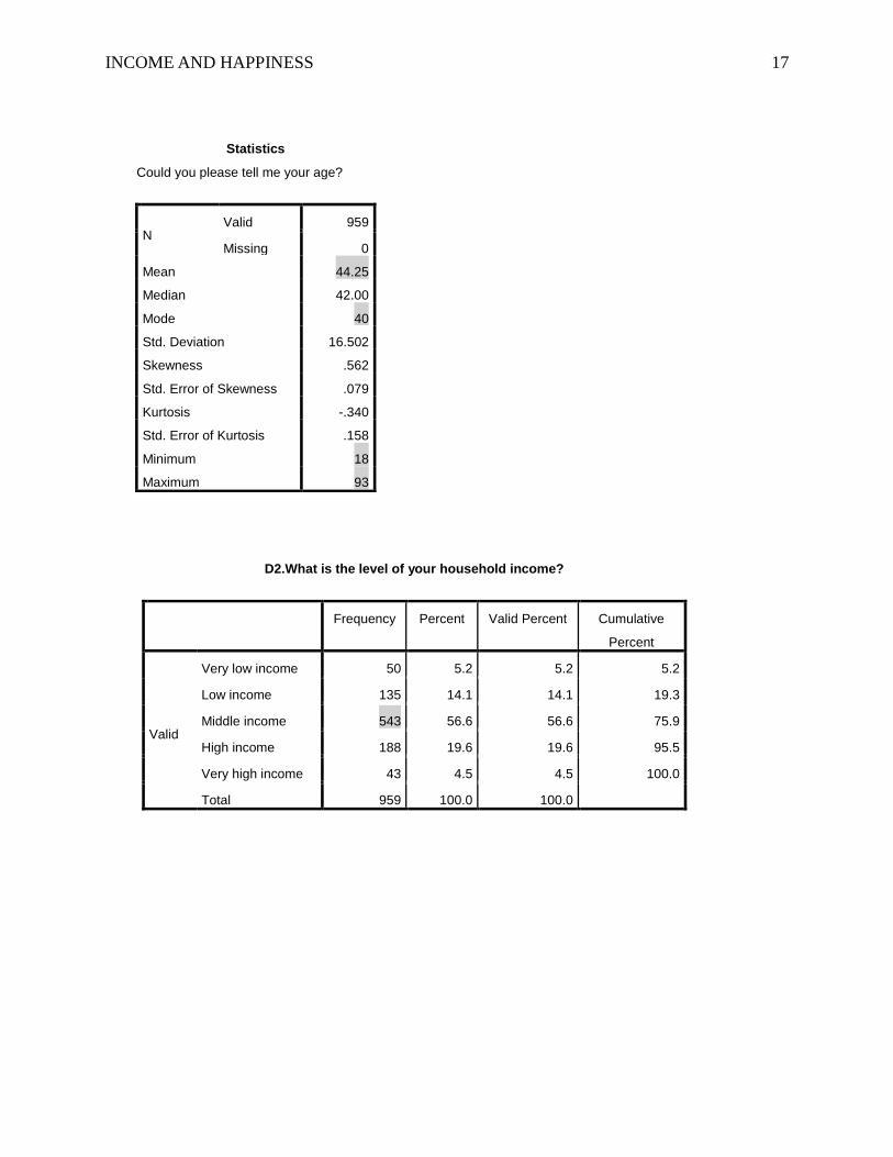
to 93. Mostly, participants were in middle adulthood, 40 years old of age, and on average, they

were 44 years old (see Appendix A).

The target population for the research study is people in the United States, so the findings

will be used to generalize people in the whole country. Accessible population in the study is

people who are living New York City.


Variables and instrumentations

Independent variable in the proposed study was income. Income was used as a factor

(independent variable) to predict happiness which was the dependent variable. Both income and

happiness were interval level data. The two variables were developed based a five-point Likert

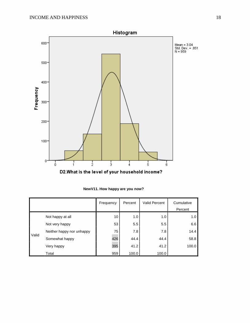
scale. Income variable’s scale consisted of “Very low income (1)”, “Low income (2)”, “Middle

income (3)”, “High income (4)” and “Very high income (5)”. For happiness variable, the scale

was originally developed by “Very happy (1)”, “Somewhat happy (2)”, “Neither happy nor

unhappy (3)”, “Not very happy (4)”, and “Not happy at all (5)”. The happiness’s scale was

inconsistent with the income’s scale because usually the more positive things should get higher

points. Therefore, the happiness’s scale was reversed to “Not happy at all (1)”, “Not very happy

(2)”, “Neither happy nor unhappy (3)”, “Somewhat happy (4)”, and “Very happy (5)”.

Analytical approach

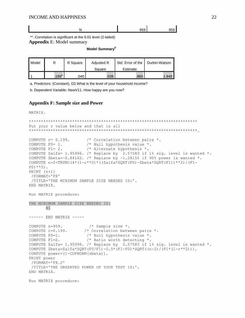
To control for type II error rate, statistical power has to be at least 0.80, and to achieve

this statistical power value, 41 participants were needed. The calculation was done by using

Power syntax for bivariate correlation on the course website (see Appendix D). The number of

participants in the study was 959, so the power value of 0.80 was satisfied.

To be able to answer the research question, simple linear regression was employed to

examine if income can be a predictor of happiness. The research study used Statistical Package

for the Social Sciences (SPSS) program to run simple linear regression. In order to be able to run

simple linear regression, the data obtained have to fulfill 6 basic assumptions:

1. Random sampling

2. Normality (Error in the dependent variable is normally distributed)


3. Homoscedasticity (The error is constant for all values of X, example constant

variance)

4. Linearity (Linear relationship exists between X and Y)

5. Independence of Errors (Error in the dependent is assumed to be uncorrelated and

independent from one another and also X)

6. Variables are measured without error (Example, Outlier)

To test if the above assumptions met, some descriptive statistics were run such as mean,

standard deviation, skewness, kurtosis, normal Q-Q plots and histograms of dependent variable

error, test of normality – Kolmogorov-Smirnov and Shapiro-Wilk, and test of homogeneity of

variance – Levene statistic.

Moreover, some inferential statistics were used in the research study to measure the

relationship between independent and dependent variables. Cook’s distance and Durbin-Watson

were used to test if outliers have leverage on the model, and if errors are correlated respectively.

Pear’s r correlation was run to test if income and happiness were related, and the effect size was

tested to measure the proportion of variation in dependent variable. Power was run to control

type II error rate and to see its percentage of achieving statistical significance. The standard error

of estimate (SEE) was measured to show the error term in the unit of analysis in the model. If

robserved > r critical, we can reject the null hypothesis and accept the alternative hypothesis, which

means there is a relationship between income and happiness, while we fail to reject the null if

robserved ≤ r critical.

Furthermore, one-way ANOVA was run to see if regression explains a significant

proportion of the variation in dependent variable. If Fobserved ≤ Fcritical, the regression does not


explain a significant proportion of the variation in dependent variable, whereas the regression

does explain a significant proportion of the variation in dependent variable if Fobserved > Fcritical.

Finally, t-tests for the population slope and population intercept were also conducted. The

t-test for the population slope was used to measure the linear relationship between income and

happiness. If tobserved > tcritical, we can reject the null hypothesis, and accept the alternative

hypothesis, and there is statistical evidence to prove that there is a linear relationship between

income and happiness (β≠0). However, if tobserved ≤ tcritical, we have to fail to reject the null

hypothesis, and there is no linear relationship between income and happiness. In addition, the t-

test for population intercept was conducted to test if the starting point is 0. If tobserved intercept >

tcritical, we can reject the null hypothesis, and accept the alternative hypothesis, which means there

is statistical evidence to prove that the starting point is not 0 (α≠0). However, if tobserved intercept ≤

tcritical, we have to fail to reject the null hypothesis, and a conclusion can be drawn that the

starting point is 0. All of the tests were measured at 0.05 alpha level.

Findings

The data were fine for simple linear regression test because they fulfilled the 6

assumptions. For the first assumption, Lee (2006) used representative random sampling to select

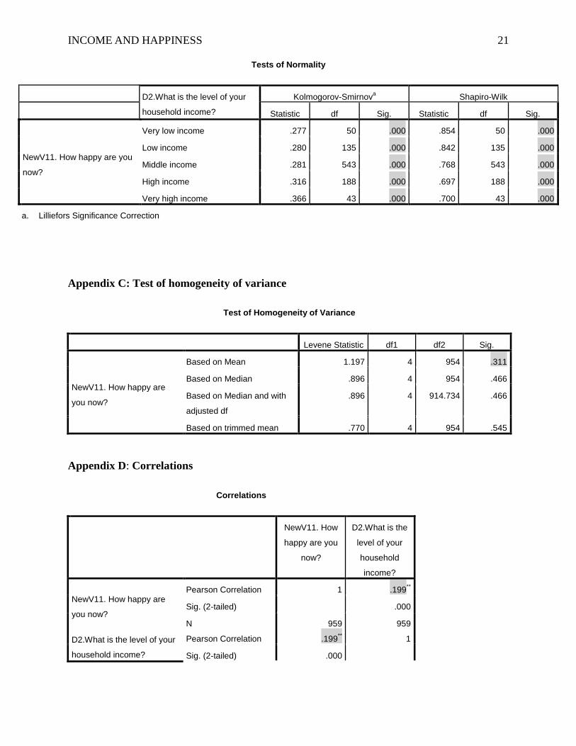
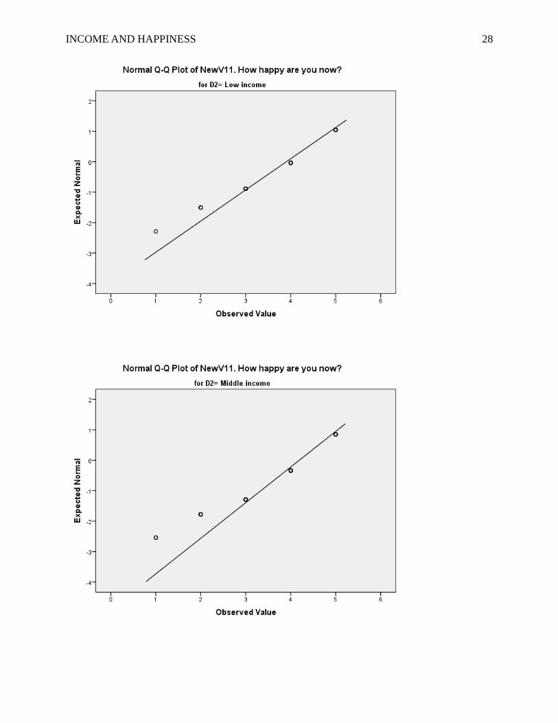
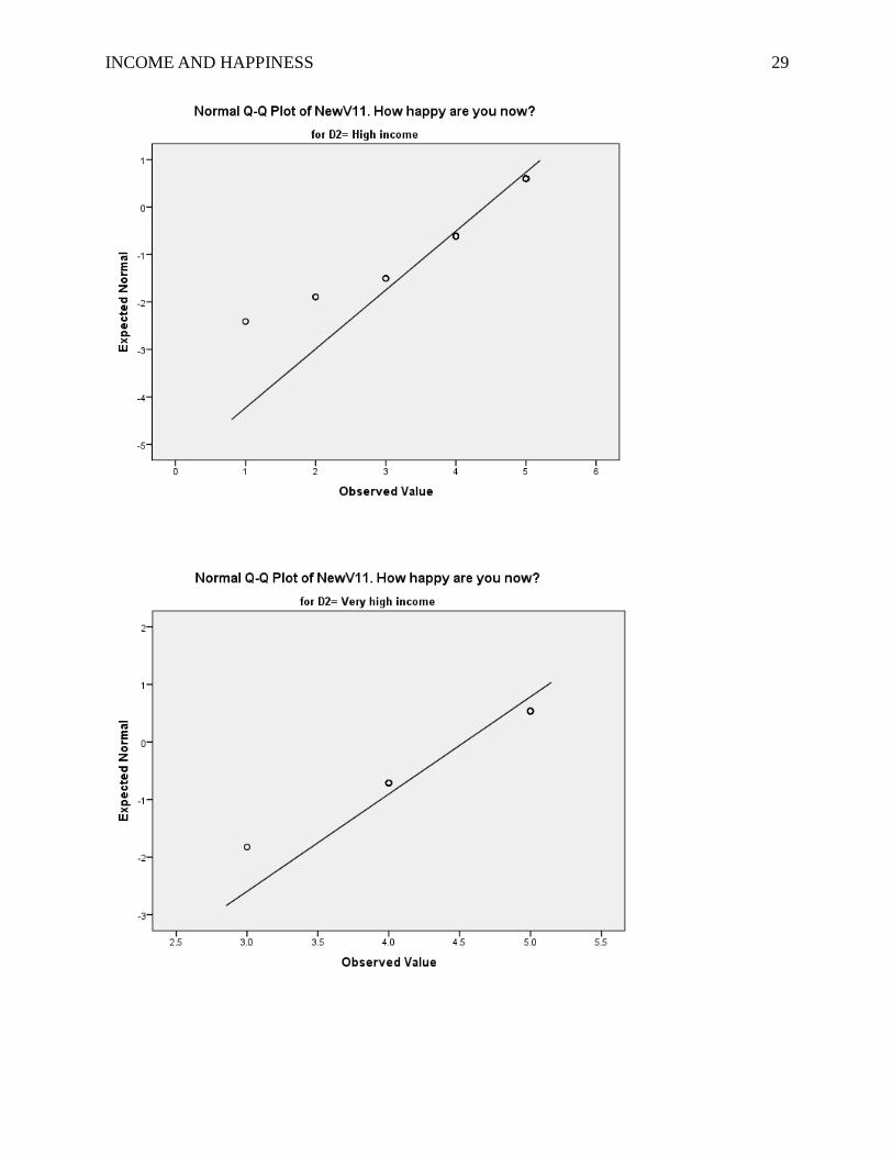
participants. Therefore, the data were fine for the first assumption. Based on the test of normality

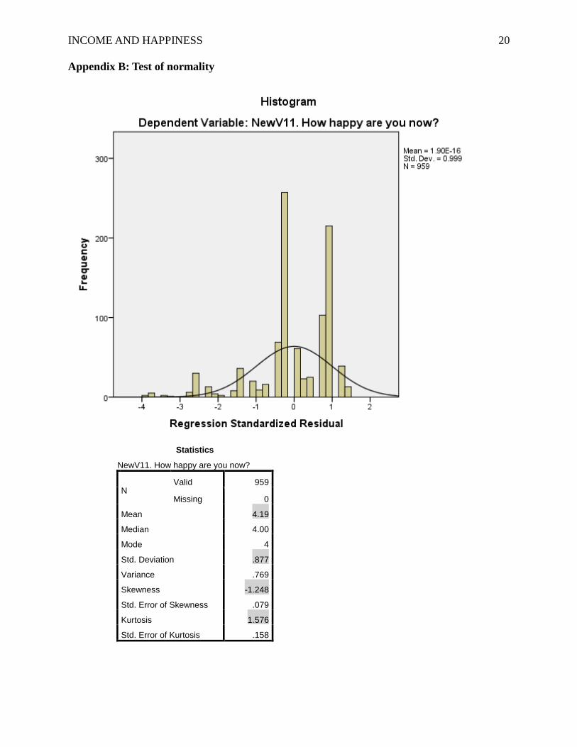
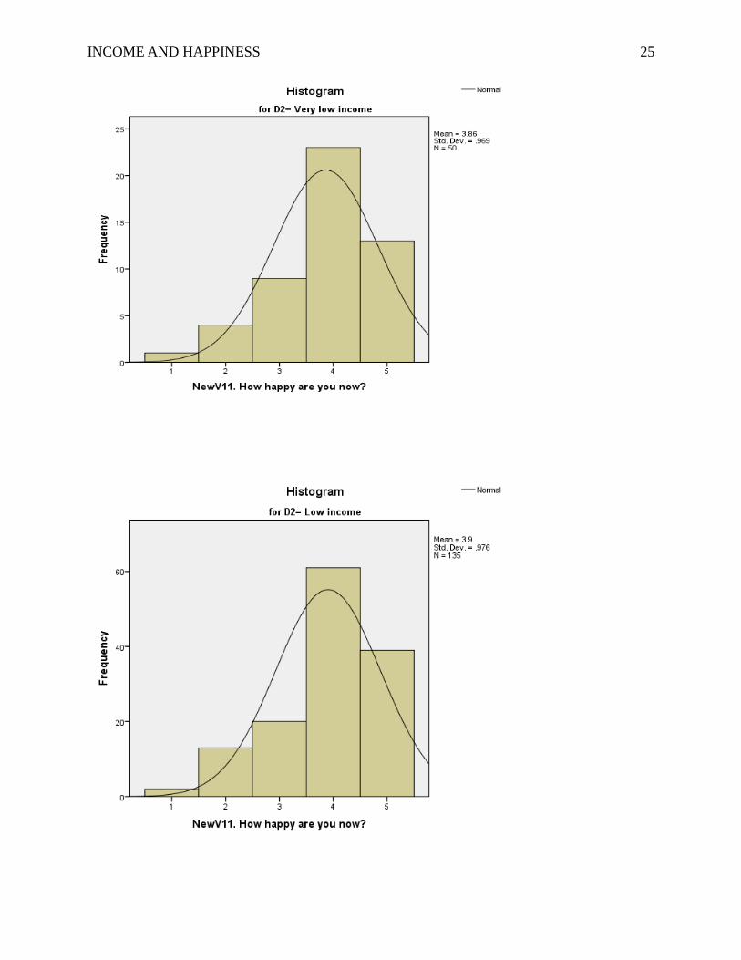
– Kolmogorov-Smirnov and Shapiro-Wilk, the results showed that Pvalue < α; however, because

the histogram indicated that errors in the dependent variable are normally distributed (see

Appendix B), and the kurtosis (1.576) and skewness (-1.248) were within the range of -2 and +2.

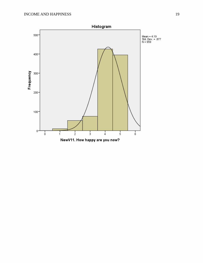
Also, mean 4.19 was bigger than standard deviation 0.877. To sum up, we could assume that the

errors in dependent variable were normally distributed. For the third assumption, the test of

homogeneity of variance was checked via the Levene statistic. The null hypothesis for the


Levene statistic test was “The variances are equal”, and the alternative hypothesis was “The

variances are not equal”. The results indicated that based on mean, Pvalue (0.311) > α (see

Appendix C), so we failed to reject the null hypothesis, which means variances in the model

were assumed equal. Hence, the third assumption was satisfied. For the fourth assumption, the t-

test for the population slope was used to measure the linear relationship between income and

happiness. The hull hypothesis for the slope was “There is no linear relationship between income

and happiness (β=0)”, and the alternative hypothesis was “There is a linear relationship between

income and happiness (β≠0)”. The results in the Coefficients table (see Appendix H) indicated

that tobserved slope value was 6.295, and Pvalue < α (0.05). At 0.05 alpha level, degree of freedom of

957, and a two-tailed test, the tcritical value was around 1.96. According to the results, tobserved slope >

tcritical, we rejected the null hypothesis, and accepted the alternative hypothesis. There was

statistical evidence to prove that there was a linear relationship between income and happiness

(β≠0). As a result, the fourth assumption was fulfilled. Based on Model summary (see Appendix

E), the Durbin Watson’s value was 1.848 (between 1.5 and 2.5), which means the error terms

from the dependent variable appeared to be uncorrelated and independent from one another. So,

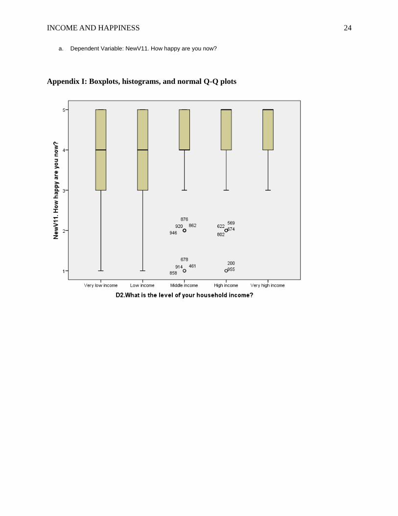
the fifth assumption was satisfied. Based on the boxplot (see Appendix I), the model has 14

outliers; however, the Cook’s distance statistic maximum value was 0.037 (see Appendix H),

which was below 1, so none of the outliers had leverage on the coefficients in the model.

Therefore, the sixth assumption was fulfilled. The results showed that all of the assumptions for

the simple linear regression test for the model were fulfilled.

The Pear’s r correction test results showed that robserved value is 0.199 significant at 0.01

alpha level (2 tailed), meaning there was a positive, slight correlation between income and

happiness (see Appendix D). The Power value which was run on the Matrix was approximate 1,


indicating that there was a 99% probability of achieving statistically significant results (see

Appendix F). The adjusted R2 value was 0.039, indicating a small effect size which means 3.9%

of the variance in someone’s happiness was accounted for by his income. The coefficient of non-

determination value for these data (1-r2) is 0.961, indicating 96.1% of the variance in someone’s

happiness was not accounted for by his income. The null hypothesis for Pear’s r correlation was

“There is no relationship between income and happiness (p=0)”, and the alternative hypothesis

was “There is a relationship between income and happiness (p≠0)”. At 0.05 alpha level, degree

of freedom of 957, and a two-tailed test, the rcritical value was approximately 0.195. With Pvalue <

α, and rcritical < robserved, we rejected the null hypothesis, and accepted the alternative hypothesis.

Hence, there was a statistically significant (positive, slight) correlation between income and

happiness. Additionally, according to the Model summary table, the standard error of the

estimate (SEE) value was 0.86 (see Appendix E). This value was the error term in the unit of

analysis in the model.

For the one-way ANOVA test, the Fobserved value was 39.627 (see Appendix G). The null

hypothesis was “Regression does not explain a significant proportion of the variation in

dependent variable (Fobserved ≤ Fcritical)”, whereas the alternative hypothesis was “Regression does

explain a significant proportion of the variation in dependent variable (Fobserved > Fcritical)”. At 0.05

alpha level, degree of freedom numerator of 1, degree of freedom denominator of 957, and a

two-tailed test, the Fcritical value was approximately 3.85. The results showed that

Fobserved(39.627)> Fcritical (3.85) and Pvalue < α. Therefore, Fobserved was beyond the critical boundary

of Fcritical. As a result, we rejected the null hypothesis, and accepted the alternative hypothesis.

We can come to a conclusion that the regression does explain a significant proportion of the

variation in dependent variable.


The hypotheses for the y-intercept were that the null hypothesis was “The starting point is

0 (α=0)”, and the alternative hypothesis was “The starting point is not 0 (α≠0)”. The t-test results

for the y-intercept showed that tobserved intercept value was 34.601 and Pvalue < α (0.05) (see

Appendix H). The same to the population slope, at 0.05 alpha level, degree of freedom of 957,

and a two-tailed test, the tcritical value was approximately 1.96. The results were tobserved intercept >

tcritical, and we rejected the null hypothesis, and accepted the alternative hypothesis. In

conclusion, there was statistical evidence to prove that the starting point was not 0 (α≠0).

At 95% confidence intervals, the slope had a lower bound value of 0.141 and an upper

bound value of 0.27, and the y-intercept had a lower bound value of 3.365, and an upper bound

value of 3.769 (see Appendix H). Both of the slope’s and the y-intercept’s intervals did not

contain 0; therefore, we rejected the null hypothesis, and accepted the alternative hypothesis. We

are confident that out of 100 trials, 95 would contain the population mean y-intercept and the

population mean slope in these intervals (estimated as 3.567 and 0.206).

The simple linear regression model is Ŷ = a + bx + E. “Ŷ” is the dependent variable

which is happiness. “x” is the independent variable income which is used to predict Ŷ. “a” is y-

intercept which is a constant term. “b” is the slope. Lastly, “E” is the random error term in the

model. According to the Coefficients table, we had slope value (b) = 0.206, and y-intercept value

(a) = 3.567, and error term value (E) = 0.86. Together, we got the simple linear regression model:

Ŷ = 3.567 + 0.206x + 0.86.

Discussion

In conclusion, the results show that there is a statistically significant positive relationship

between income and happiness; however, the relationship is really weak, which is consistent with

the previous research studies (Howell & Howell, 2008 as cited in Boyce et al, 2010; Easterlin,


2001). Therefore, people with higher income are slightly happier than those who have less. In

other words, people with less income are slightly less happy than those who have more. The

study confirms Easterlin’s theory that over life time, happiness tends to remain stable in spite of

income growth. People will not be much happier despite the fact that they have more money in

the future. A main implication from this findings is that having more money does not make

people much happier.

The study also shows that there is statistical evidence to prove that there is a linear

relationship between income and happiness, and the starting point is not 0. For each increase of 1

point in income level, the model predicts that the expected level of happiness is estimated to

increase by 0.206 or 1/5 of a happiness point, with the starting happiness level for the sample of

3.567 scale points. Based on these results, it can be concluded that income is not a good predictor

of happiness.

There is a threat to internal validity regarding the instrumentation of the study. The word

“happiness” is a construct. It is hard for participants to rate how happy they are directly. Instead,

there should be operational definitions for the term happiness so that participants find it easier to

answer the question. Additionally, income variable was developed by using interval

measurement, which means participants were requested to rate their level of income in five

different levels: very low income, low income, middle income, high income, or very high

income. It is challenging for participants to rate their levels of income. The participants may not

be sure of which levels they are in. It also depends on to whom participants compare their

income. If they compare their income to very rich people, then they would rate their income low

or even very low. In contrast, if they compare their income to very poor people, they would rate


high or very high income. Hence, the instrument would be more accurate and valid if the

participants are asked to tell their exact income.

The limitation of the study is that it can only prove the correlation between income and

happiness, but not causation. The research study cannot tell if income is the cause of happiness.

Furthermore, as income is slightly related to happiness, future research should extensively focus

on more independent variables in the study such as age, health, education and employment.


References

Boyce, C. J., Brown, G. D. A., & Moore, S. C. (2010). Money and happiness: Rank of income,

not income, affects life satisfaction. Psychological Science, 21(4), 471-475.

Doi: 10.1177/0956797610362671

Como, M. (2011). Do happier people make more money? An empirical study of the effect of a

person’s happiness on their income. The Park Place Economist, 19. Retrieved from:

http://www.iwu.edu/economics/PPE19/1Como.pdf

Easterlin, R. A. (2001). Income and happiness: Towards a unified theory. The Economic Journal,

111 (July), 465-484. Retrieved from:

http://www.uvm.edu/~pdodds/files/papers/others/2001/easterlin2001a.pdf

Lee, N. Y. (2006). Assessing happiness and competitiveness of world major metropolises, 2006.

Inter-University Consortium For Political And Social Research, 27901. Retrieved from:

http://www.icpsr.umich.edu/icpsrweb/ICPSR/studies/27901


Appendices

Appendix A: Gender, age, income and happiness

Gender

Frequency Percent Valid Percent Cumulative

Percent

Valid

Male 457 47.7 47.7 47.7

Female 502 52.3 52.3 100.0

Total 959 100.0 100.0


Statistics

Could you please tell me your age?

N Valid 959

Missing 0

Mean 44.25

Median 42.00

Mode 40

Std. Deviation 16.502

Skewness .562

Std. Error of Skewness .079

Kurtosis -.340

Std. Error of Kurtosis .158

Minimum 18

Maximum 93

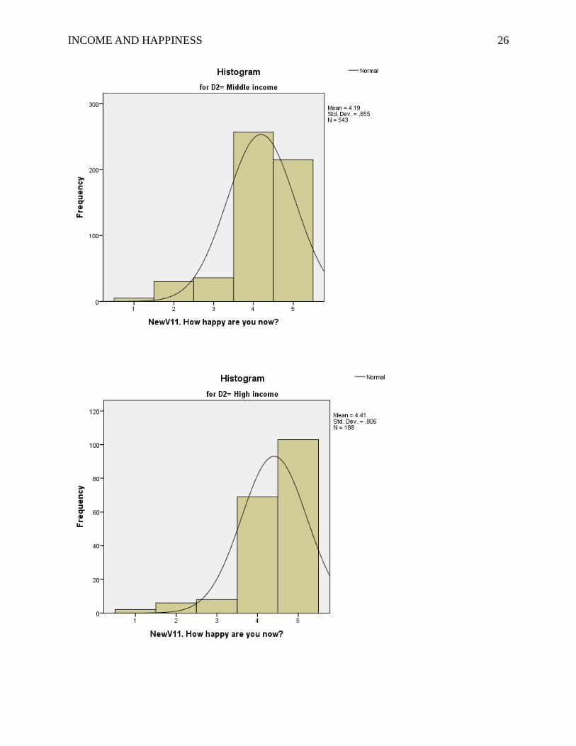
D2.What is the level of your household income?


Percent

Valid

Very low income 50 5.2 5.2 5.2

Low income 135 14.1 14.1 19.3

Middle income 543 56.6 56.6 75.9

High income 188 19.6 19.6 95.5

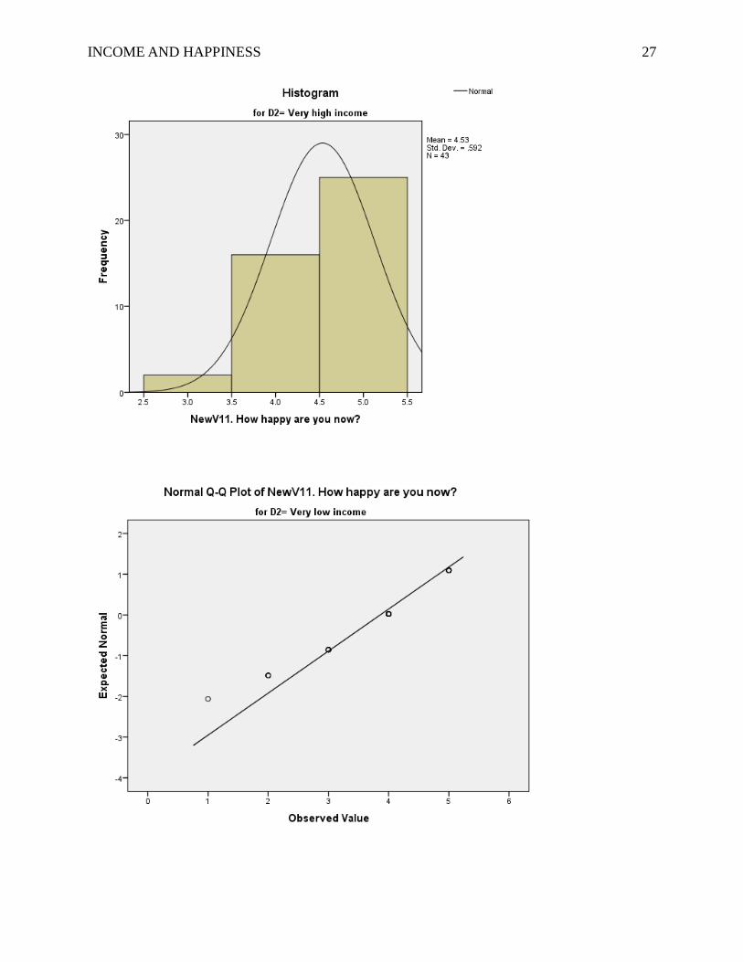
Very high income 43 4.5 4.5 100.0

Total 959 100.0 100.0


NewV11. How happy are you now?


Percent

Valid

Not happy at all 10 1.0 1.0 1.0

Not very happy 53 5.5 5.5 6.6

Neither happy nor unhappy 75 7.8 7.8 14.4

Somewhat happy 426 44.4 44.4 58.8

Very happy 395 41.2 41.2 100.0

Total 959 100.0 100.0



Appendix B: Test of normality

Statistics

NewV11. How happy are you now?

N Valid 959

Missing 0

Mean 4.19

Median 4.00

Mode 4

Std. Deviation .877

Variance .769

Skewness -1.248

Std. Error of Skewness .079

Kurtosis 1.576

Std. Error of Kurtosis .158


Appendix C: Test of homogeneity of variance

Test of Homogeneity of Variance

Levene Statistic df1 df2 Sig.

NewV11. How happy are

you now?

Based on Mean 1.197 4 954 .311

Based on Median .896 4 954 .466

Based on Median and with

adjusted df

.896 4 914.734 .466

Based on trimmed mean .770 4 954 .545

Appendix D: Correlations

Correlations

NewV11. How

happy are you

now?

D2.What is the

level of your

household

income?

NewV11. How happy are

you now?

Pearson Correlation 1 .199**

Sig. (2-tailed) .000

N 959 959

D2.What is the level of your

household income?

Pearson Correlation .199** 1

Sig. (2-tailed) .000

Tests of Normality


household income?

Kolmogorov-Smirnova Shapiro-Wilk

Statistic df Sig. Statistic df Sig.

NewV11. How happy are you

now?

Very low income .277 50 .000 .854 50 .000

Low income .280 135 .000 .842 135 .000

Middle income .281 543 .000 .768 543 .000

High income .316 188 .000 .697 188 .000

Very high income .366 43 .000 .700 43 .000

a. Lilliefors Significance Correction


N 959 959

**. Correlation is significant at the 0.01 level (2-tailed).

Appendix E: Model summary

Model Summaryb

Model R R Square Adjusted R

Square

Std. Error of the

Estimate

Durbin-Watson

1 .199a .040 .039 .860 1.848

a. Predictors: (Constant), D2.What is the level of your household income?

b. Dependent Variable: NewV11. How happy are you now?

Appendix F: Sample size and Power

MATRIX.

**********************************************************************

Put your r value below and that is all

**********************************************************************.

COMPUTE r= 0.199. /* Correlation between pairs *.

COMPUTE F0= 1. /* Null hypothesis value *.

COMPUTE F1= 2. /* Alternate hypothesis *.

COMPUTE Zalfa= 1.95996. /* Replace by 2.57583 if 1% sig. level is wanted *.

COMPUTE Zbeta=-0.84162. /* Replace by -1.28155 if 90% power is wanted *.

COMPUTE n=2+TRUNC(4*(1-r**2)*((Zalfa*SQRT(F0)-Zbeta*SQRT(F1))**2)/(F1-

F0)**2).

PRINT {n+1}

/FORMAT='F8'

/TITLE='THE MINIMUM SAMPLE SIZE NEEDED IS:'.

END MATRIX.

Run MATRIX procedure:

THE MINIMUM SAMPLE SIZE NEEDED IS:

41

------ END MATRIX -----

COMPUTE n=959. /* Sample size *.

COMPUTE r=0.199. /* Correlation between pairs *.

COMPUTE F0=1. /* Null hypothesis value *.

COMPUTE F1=2. /* Ratio worth detecting *.

COMPUTE Zalfa= 1.95996. /* Replace by 2.57583 if 1% sig. level is wanted *.

COMPUTE Zbeta=Zalfa*SQRT(F0/F1)-0.5*(F1-F0)*SQRT((n-2)/(F1*(1-r**2))).

COMPUTE power=(1-CDFNORM(zbeta)).

PRINT power

/FORMAT='F8.2'

/TITLE='THE OBSERVED POWER OF YOUR TEST IS:'.

END MATRIX.

Run MATRIX procedure:


THE OBSERVED POWER OF YOUR TEST IS:

1.00

Appendix G: ANOVA

ANOVAa

Model Sum of Squares df Mean Square F Sig.

1

Regression 29.292 1 29.292 39.627 .000b

Residual 707.405 957 .739

Total 736.697 958

a. Dependent Variable: NewV11. How happy are you now?

b. Predictors: (Constant), D2.What is the level of your household income?

Appendix H: Coefficients and residuals statistics

Residuals Statisticsa

Minimum Maximum Mean Std. Deviation N

Predicted Value 3.77 4.59 4.19 .175 959

Std. Predicted Value -2.399 2.303 .000 1.000 959

Standard Error of Predicted Value .028 .072 .037 .013 959

Adjusted Predicted Value 3.76 4.61 4.19 .175 959

Residual -3.389 1.228 .000 .859 959

Std. Residual -3.942 1.428 .000 .999 959

Stud. Residual -3.947 1.433 .000 1.001 959

Deleted Residual -3.397 1.236 .000 .861 959

Stud. Deleted Residual -3.977 1.434 -.001 1.002 959

Mahal. Distance .002 5.753 .999 1.620 959

Cook's Distance .000 .037 .001 .002 959

Centered Leverage Value .000 .006 .001 .002 959

Coefficientsa

Model Unstandardized

Coefficients

Standardized

Coefficients

t Sig. 95.0% Confidence Interval for B

B Std. Error Beta Lower Bound Upper Bound

1

(Constant) 3.567 .103 34.601 .000 3.365 3.769


household income?

.206 .033 .199 6.295 .000 .141 .270




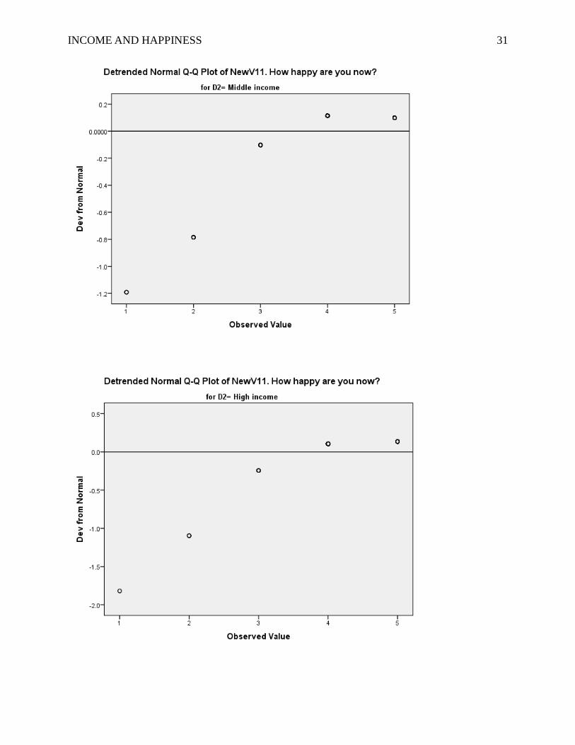
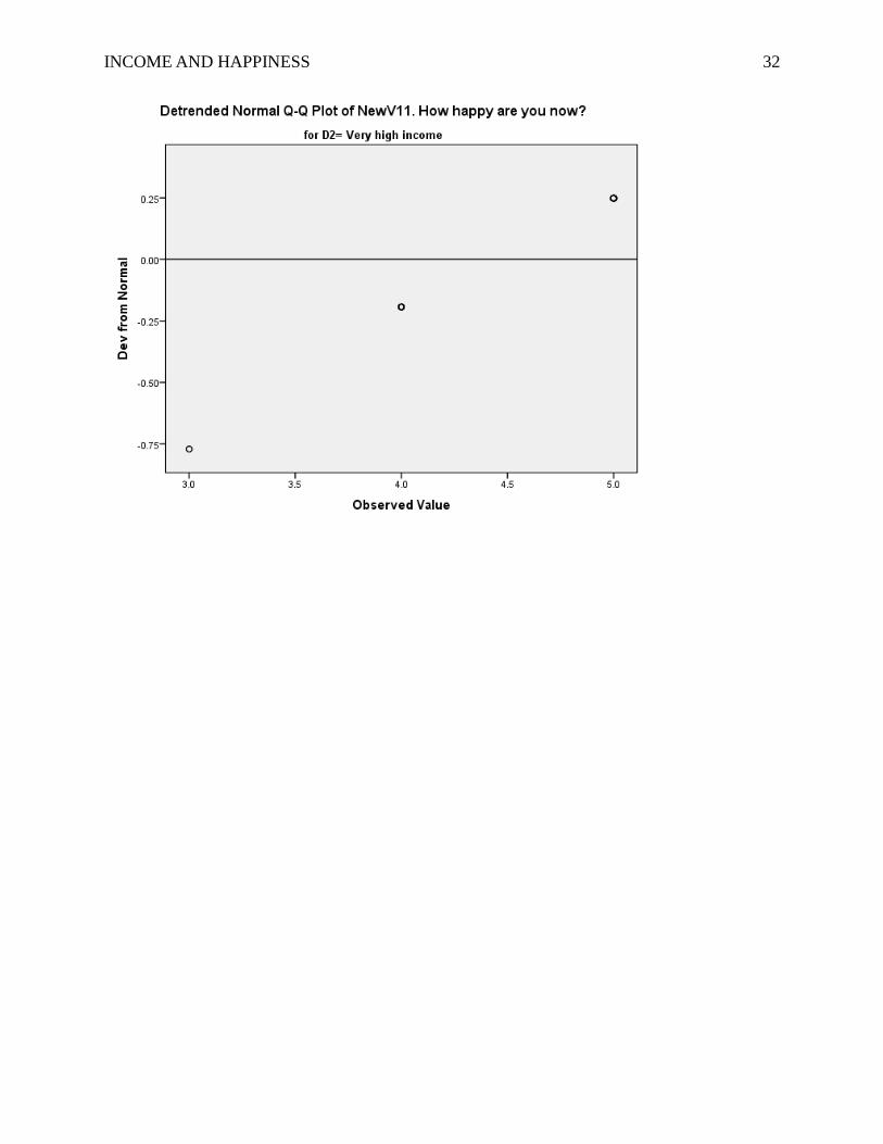
Appendix I: Boxplots, histograms, and normal Q-Q plots









Documents

Income and Happiness - NIU College of Educationcedu.niu.edu/~walker/statistics/K-12 Simple Linear Regression.pdf · The research study employed simple linear regression analysis to