Regression 9.1 Simple Linear Regression - Calvin Collegerpruim/courses/m145/F14/Notes/Regression.pdf · Estimate the slope and intercept of your line by reading them oﬀof the graph

Regression 137

9Regression

9.1 Simple Linear Regression

9.1.1 The Least Squares Method

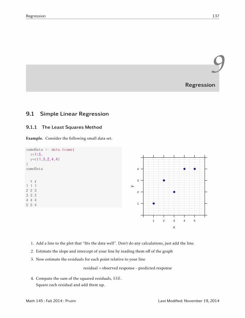
Example. Consider the following small data set.

someData <- data.frame(

x=1:5,

y=c(1,3,2,4,4)

)

someData

x y

1 1 1

2 2 3

3 3 2

4 4 4

5 5 4

x

y

1

2

3

4

1 2 3 4 5

●

●

●

● ●

1. Add a line to the plot that “fits the data well”. Don’t do any calculations, just add the line.

2. Estimate the slope and intercept of your line by reading them off of the graph

3. Now estimate the residuals for each point relative to your line

residual = observed response−predicted response

4. Compute the sum of the squared residuals, SSE.

Square each residual and add them up.

Math 145 : Fall 2014 : Pruim Last Modified: November 19, 2014

138 Regression

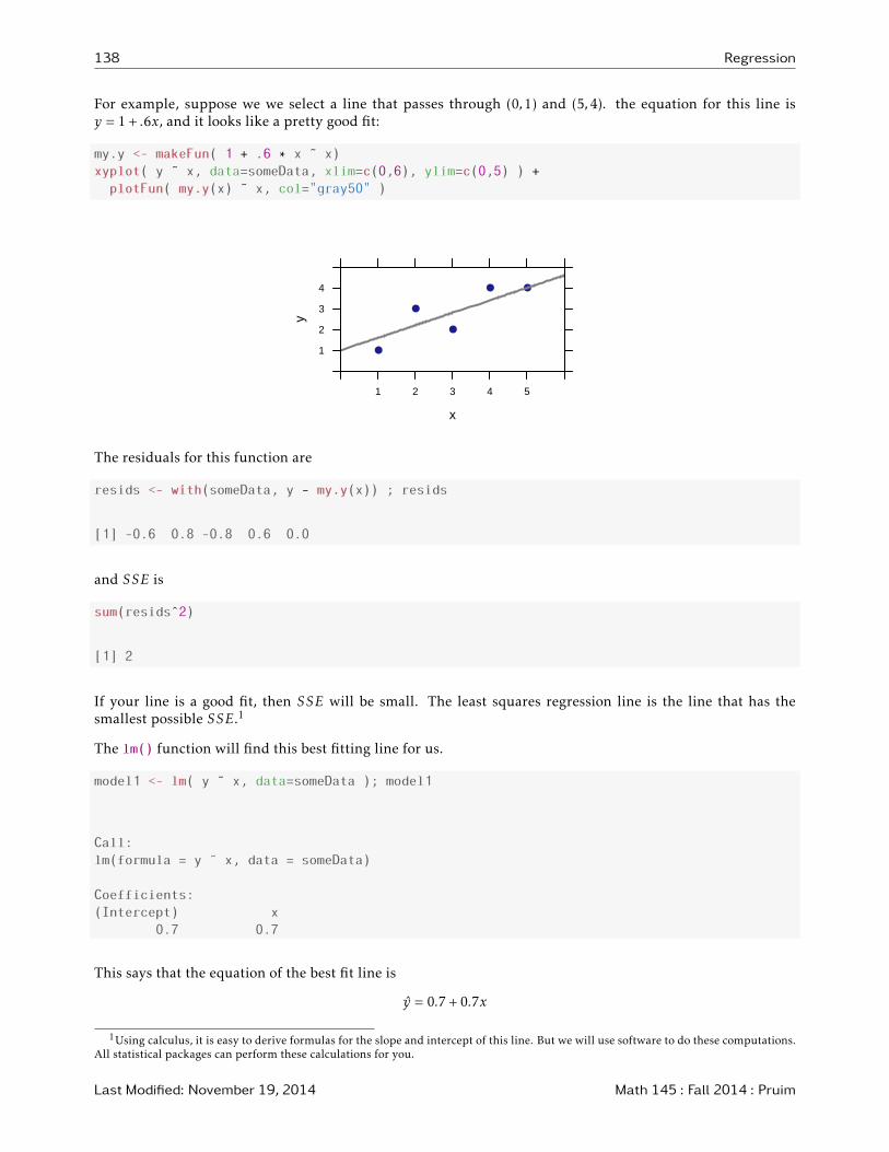
For example, suppose we we select a line that passes through (0,1) and (5,4). the equation for this line isy = 1+ .6x, and it looks like a pretty good fit:

my.y <- makeFun( 1 + .6 * x ˜ x)

xyplot( y ˜ x, data=someData, xlim=c(0,6), ylim=c(0,5) ) +

plotFun( my.y(x) ˜ x, col="gray50" )

x

y

1

2

3

4

1 2 3 4 5

●

●

●

● ●

The residuals for this function are

resids <- with(someData, y - my.y(x)) ; resids

[1] -0.6 0.8 -0.8 0.6 0.0

and SSE is

sum(residsˆ2)

[1] 2

If your line is a good fit, then SSE will be small. The least squares regression line is the line that has thesmallest possible SSE.1

The lm() function will find this best fitting line for us.

model1 <- lm( y ˜ x, data=someData ); model1

Call:

lm(formula = y ˜ x, data = someData)

Coefficients:

(Intercept) x

0.7 0.7

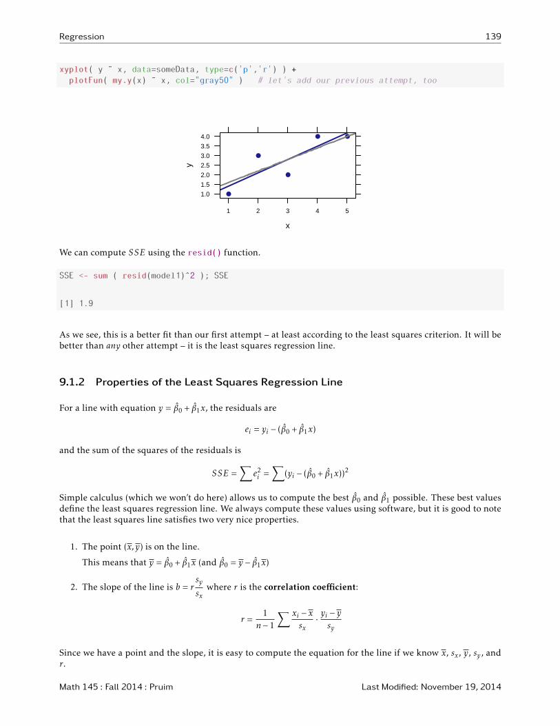
This says that the equation of the best fit line is

y = 0.7+0.7x

1Using calculus, it is easy to derive formulas for the slope and intercept of this line. But we will use software to do these computations.All statistical packages can perform these calculations for you.

Last Modified: November 19, 2014 Math 145 : Fall 2014 : Pruim

Regression 139

xyplot( y ˜ x, data=someData, type=c('p','r') ) +

plotFun( my.y(x) ˜ x, col="gray50" ) # let's add our previous attempt, too

x

y1.0

1.5

2.0

2.5

3.0

3.5

4.0

1 2 3 4 5

●

●

●

● ●

We can compute SSE using the resid() function.

SSE <- sum ( resid(model1)ˆ2 ); SSE

[1] 1.9

As we see, this is a better fit than our first attempt – at least according to the least squares criterion. It will bebetter than any other attempt – it is the least squares regression line.

9.1.2 Properties of the Least Squares Regression Line

For a line with equation y = β0 + β1x, the residuals are

ei = yi − (β0 + β1x)

and the sum of the squares of the residuals is

SSE =∑

e2i =∑

(yi − (β0 + β1x))2

Simple calculus (which we won’t do here) allows us to compute the best β0 and β1 possible. These best valuesdefine the least squares regression line. We always compute these values using software, but it is good to notethat the least squares line satisfies two very nice properties.

1. The point (x,y) is on the line.

This means that y = β0 + β1x (and β0 = y − β1x)

2. The slope of the line is b = rsy

sxwhere r is the correlation coefficient:

r =1

n− 1

∑ xi − x

sx·yi − y

sy

Since we have a point and the slope, it is easy to compute the equation for the line if we know x, sx, y, sy , andr.


140 Regression

9.1.3 Explanatory and Response Variables Matter

It is important that the explanatory variable be the “x” variable and the response variable be the “y” variablewhen doing regression. If we reverse the roles of y and x we do not get the same model. This is because theresiduals are measured vertically (in the y direction).

9.1.4 Example: Florida Lakes Example

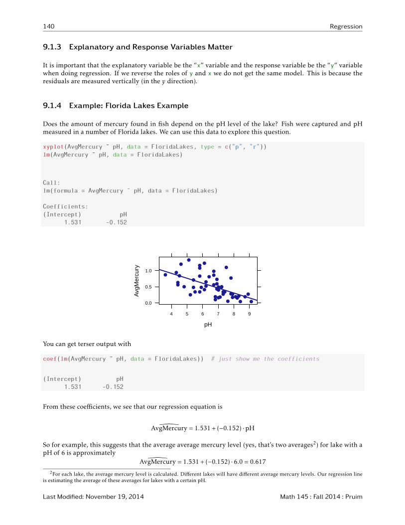
Does the amount of mercury found in fish depend on the pH level of the lake? Fish were captured and pHmeasured in a number of Florida lakes. We can use this data to explore this question.

xyplot(AvgMercury ˜ pH, data = FloridaLakes, type = c("p", "r"))

lm(AvgMercury ˜ pH, data = FloridaLakes)

Call:

lm(formula = AvgMercury ˜ pH, data = FloridaLakes)

Coefficients:

(Intercept) pH

1.531 -0.152

pH

Avg

Mer

cury

0.0

0.5

1.0

4 5 6 7 8 9

●●

●

●

●

●

●

●

● ●●

●●

●

●● ●

●

●●

●●

●

●

●

●

●

●

●● ●●

●

●

●●●●

●

●

●●

●

●

●

●●

●

●

●●

● ●

You can get terser output with

coef(lm(AvgMercury ˜ pH, data = FloridaLakes)) # just show me the coefficients

(Intercept) pH

1.531 -0.152

From these coefficients, we see that our regression equation is

�AvgMercury = 1.531+ (−0.152) ·pH

So for example, this suggests that the average average mercury level (yes, that’s two averages2) for lake with apH of 6 is approximately

�AvgMercury = 1.531+ (−0.152) · 6.0 = 0.617

2For each lake, the average mercury level is calculated. Different lakes will have different average mercury levels. Our regression lineis estimating the average of these averages for lakes with a certain pH.


Regression 141

Using makeFun(), we can automate computing the estimated response:

Mercury.model <- lm(AvgMercury ˜ pH, data = FloridaLakes)

estimated.AvgMercury <- makeFun(Mercury.model)

estimated.AvgMercury(6)

1

0.617

9.1.5 Example: Inkjet Printers

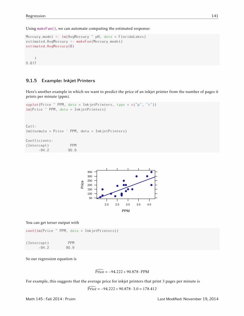
Here’s another example in which we want to predict the price of an inkjet printer from the number of pages itprints per minute (ppm).

xyplot(Price ˜ PPM, data = InkjetPrinters, type = c("p", "r"))

lm(Price ˜ PPM, data = InkjetPrinters)

Call:

lm(formula = Price ˜ PPM, data = InkjetPrinters)

Coefficients:

(Intercept) PPM

-94.2 90.9

PPM

Pric

e

50

100

150

200

250

300

350

2.0 2.5 3.0 3.5 4.0

●

●

●

●

●

●

●

●

● ●

●●●

●

●

●

●

●

●

●

You can get terser output with

coef(lm(Price ˜ PPM, data = InkjetPrinters))

(Intercept) PPM

-94.2 90.9

So our regression equation is

�Price = −94.222+90.878 ·PPM

For example, this suggests that the average price for inkjet printers that print 3 pages per minute is

�Price = −94.222+90.878 · 3.0 = 178.412


142 Regression

9.2 Parameter Estimates

9.2.1 Interpreting the Coefficients

The coefficients of the linear model tell us how to construct the linear function that we use to estimate responsevalues, but they can be interesting in their own rite as well.

The intercept β0 is the mean response value when the explanatory variable is 0. This may or may not beinteresting. Often β0 is not interesting because we are not interested in the value of the response variablewhen the predictor is 0. (That might not even be a possible value for the predictor.) Furthermore, if we do notcollect data with values of the explanatory variable near 0, then we will be extrapolating from our data whenwe talk about the intercept.

The estimate for β1, on the other hand, is nearly always of interest. The slope coefficient β1 tells us howquickly the response variable changes per unit change in the predictor. This is an interesting value in manymore situations. Furthermore, when β1 = 0, then our model says that the average response does not depend onthe predictor at all. So when 0 is contained in the confidence interval for β1 or we cannot rejectH0: β1 = 0, thenwe do not have sufficient evidence to be convinced that our predictor is of any use in predicting the response.

Since β1 = rsysx, testing whether β1 = 0 is equivalent to testing whether correlation coefficient ρ = 0.

9.2.2 Estimating σ

There is one more parameter in our model that we have been mostly ignoring so far: σ (or equivalently σ2).This is the parameter that describes how tightly things should cluster around the regression line. We canestimate σ2 from our residuals:

σ2 =MSE =

∑i e

2i

n− 2

σ = RMSE =√MSE =

√∑i e

2i

n− 2

The acronymsMSE and RMSE stand forMean Squared Error and Root Mean Squared Error. The numeratorin these expressions is the sum of the squares of the residuals

SSE =∑

i

e2i .

This is precisely the quantity that we were minimizing to get our least squares fit.

MSE =SSE

DFE

where DFE = n − 2 is the degrees of freedom associated with the estimation of σ2 in a simple linear model.We lose two degrees of freedom when we estimate β0 and β1, just like we lost 1 degree of freedom when wehad to estimate µ in order to compute a sample variance.

RMSE =√MSE is listed in the summary output for the linear model as the residual standard error because

it is the estimated standard deviation of the error terms in the model.

summary(Mercury.model)


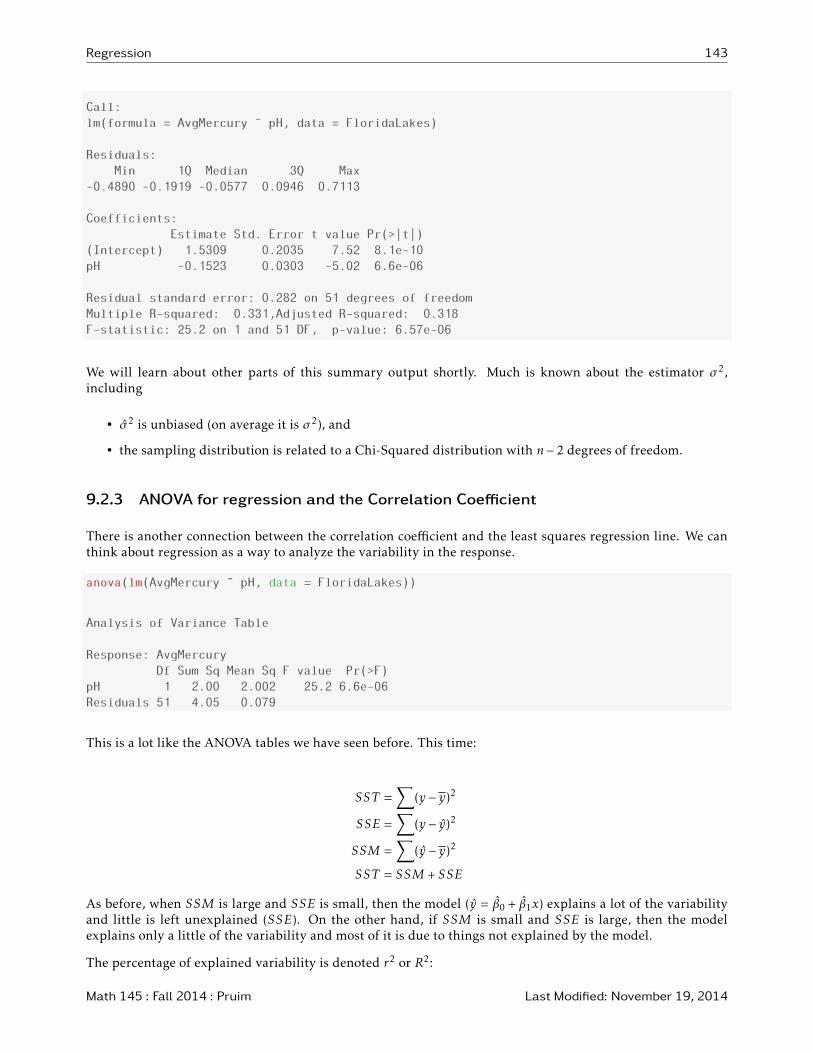
Regression 143

Call:


Residuals:

Min 1Q Median 3Q Max

-0.4890 -0.1919 -0.0577 0.0946 0.7113

Coefficients:

Estimate Std. Error t value Pr(>|t|)

(Intercept) 1.5309 0.2035 7.52 8.1e-10

pH -0.1523 0.0303 -5.02 6.6e-06

Residual standard error: 0.282 on 51 degrees of freedom

Multiple R-squared: 0.331,Adjusted R-squared: 0.318

F-statistic: 25.2 on 1 and 51 DF, p-value: 6.57e-06

We will learn about other parts of this summary output shortly. Much is known about the estimator σ2,including

• σ2 is unbiased (on average it is σ2), and

• the sampling distribution is related to a Chi-Squared distribution with n− 2 degrees of freedom.

9.2.3 ANOVA for regression and the Correlation Coefficient

There is another connection between the correlation coefficient and the least squares regression line. We canthink about regression as a way to analyze the variability in the response.

anova(lm(AvgMercury ˜ pH, data = FloridaLakes))

Analysis of Variance Table

Response: AvgMercury

Df Sum Sq Mean Sq F value Pr(>F)

pH 1 2.00 2.002 25.2 6.6e-06

Residuals 51 4.05 0.079

This is a lot like the ANOVA tables we have seen before. This time:

SST =∑

(y − y)2

SSE =∑

(y − y)2

SSM =∑

(y − y)2

SST = SSM + SSE

As before, when SSM is large and SSE is small, then the model (y = β0 + β1x) explains a lot of the variabilityand little is left unexplained (SSE). On the other hand, if SSM is small and SSE is large, then the modelexplains only a little of the variability and most of it is due to things not explained by the model.

The percentage of explained variability is denoted r2 or R2:


144 Regression

R2 =SSM

SST=

SSM

SSM + SSE

For our the Florida lakes study, we see that

• SSM = 2.00

• SSE = 4.05

• SST = 2.00+4.05 = 6.05

• R2 = SSMSST = 2

6.05 = 0.331

This number is listed as “Multiple R-squared” on the summary output.

So pH explains roughly 1/3 of the variability in mercury levels. The other two thirds of the variabilityin mercury levels is due to other things. (We can think of many things that might matter: size of thelake, depth of the lake, types of fish in the lake, types of plants in the lake, proximity to industrialization– highways, streets, manufacturing plants, etc.) More complex studies might investigate the effects ofseveral such factors simultaneously.

The correlation coefficient

The square root of R2 (with a sign to indicate whether the association between explanatory and responsevariables is positive or negative) is the correlation coefficient, R (or r). As a reminder, here are some importantfacts about R:

1. R is always between -1 and 1

2. R is 1 or -1 only if all the dots fall exactly on a line.

3. If the relationship between the explanatory and response variables is not roughly linear, then R is not avery useful number. (And simple linear regression is not very useful either).

4. For linear relationships, R is a measure of the strength of the relationship. If R is close to 1 or -1, thelinear association is strong. If it is closer to 0, the linear association is weak (with lots of scatter about thebest fit line).

5. R is unitless – if we change the units of our measurements (from English to metric, for example) it willnot affect the value of R.

9.3 Confidence Intervals and Hypothesis Tests

9.3.1 Bootstrap

So how good are these estimates? We would like have interval estimates rather than just point estimates. Oneway to get interval estimates for the coefficients is to use the bootstrap.

Florida Lakes

boot.lakes <- do(1000) * lm(AvgMercury ˜ pH, data = resample(FloridaLakes))

head(boot.lakes, 2)


Regression 145

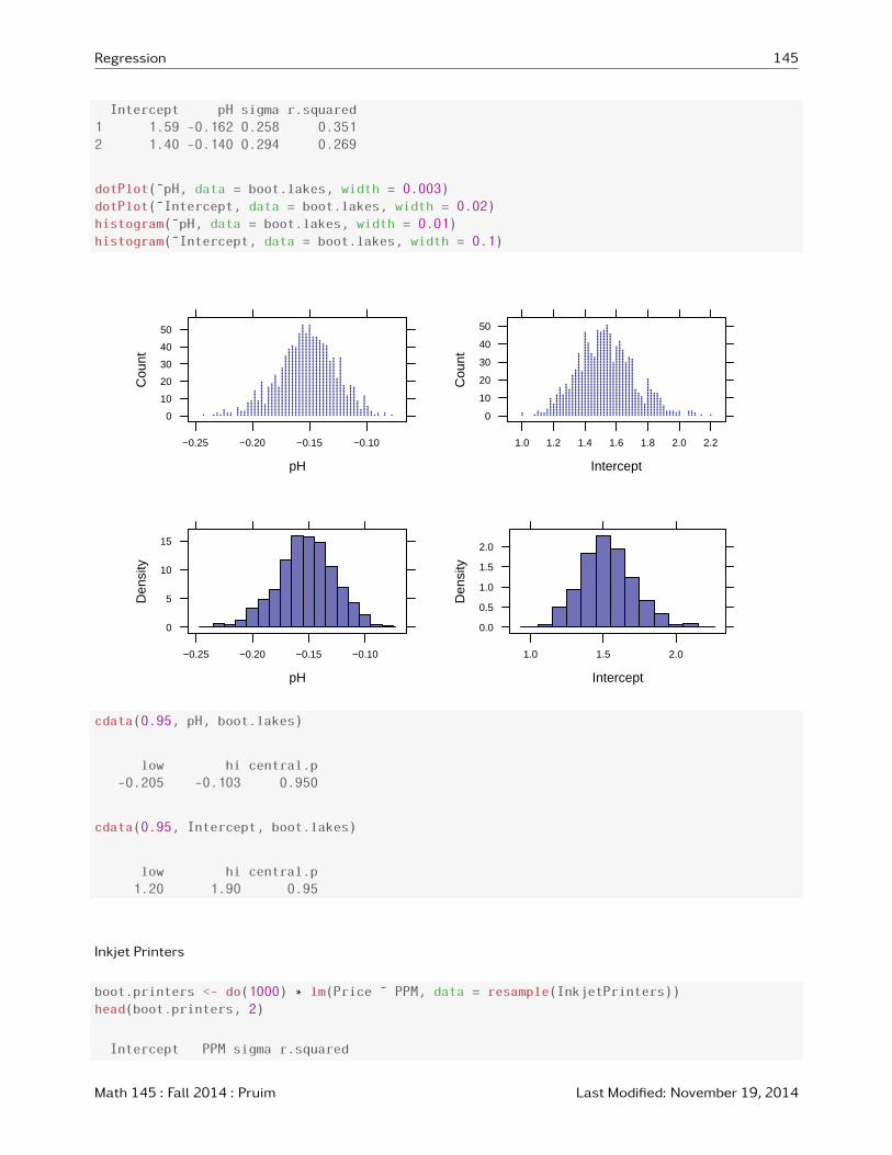
Intercept pH sigma r.squared

1 1.59 -0.162 0.258 0.351

2 1.40 -0.140 0.294 0.269

dotPlot(˜pH, data = boot.lakes, width = 0.003)

dotPlot(˜Intercept, data = boot.lakes, width = 0.02)

histogram(˜pH, data = boot.lakes, width = 0.01)

histogram(˜Intercept, data = boot.lakes, width = 0.1)

pH

Cou

nt

0

10

20

30

40

50

−0.25 −0.20 −0.15 −0.10

● ● ●●

● ●●●●

●●

●●

●●●●●

●●●

●●●

●●●●●●●●

●●●●●●●●●

●●●●●●●●●●●●●●●

●●●●●●●●●

●●●●●●●●●●●●●●●●●●●●

●●●●●●●

●●●●●●●●●●●●●●●●●

●●●●●●●●●●●●●●●●●●●

●●●●●●●●●●●●●●●●●●●●●●●●

●●●●●●●●●●●●●●●●●

●●●●●●●●●●●●●●●●●●●●●●●●●●●●

●●●●●●●●●●●●●●●●●●●●●●●●●●●●●●●●●●●

●●●●●●●●●●●●●●●●●●●●●●●●●●●●●●●●●●●●●●●

●●●●●●●●●●●●●●●●●●●●●●●●●●●●●●●●●●●●●●●●●

●●●●●●●●●●●●●●●●●●●●●●●●●●●●●●●●●●●●●●●●

●●●●●●●●●●●●●●●●●●●●●●●●●●●●●●●●●●●●●●●●●●●●●●●●

●●●●●●●●●●●●●●●●●●●●●●●●●●●●●●●●●●●●●●●●●●●●●●●●●●●●●

●●●●●●●●●●●●●●●●●●●●●●●●●●●●●●●●●●●●●●●●●●●●●●●●

●●●●●●●●●●●●●●●●●●●●●●●●●●●●●●●●●●●●●●●●●●●●●●●●●●●●●

●●●●●●●●●●●●●●●●●●●●●●●●●●●●●●●●●●●●●●●●●●●●●●

●●●●●●●●●●●●●●●●●●●●●●●●●●●●●●●●●●●●●●●●●●●●●●

●●●●●●●●●●●●●●●●●●●●●●●●●●●●●●●●●●●●●●●●●●●●

●●●●●●●●●●●●●●●●●●●●●●●●●●●●●●●●●●●●●●●●●●

●●●●●●●●●●●●●●●●●●●●●●●●●●●●●●●●●●●●●●●●●

●●●●●●●●●●●●●●●●●●●●●●●●●●●●●●●●

●●●●●●●●●●●●●●●●●●●●●●●●●●●●●●●●●●

●●●●●●●●●●●●●●●●●●●●●●

●●●●●●●●●●●●●●●●●●●●●●●●●●●●●●●●●●

●●●●●●●●●●●●●●●●●●

●●●●●●●●●●●●

●●●●●●●●●●●●●●●●●●

●●●●●●●●●●●●●●●●●

●●●●●●●●●

●●●●

●●●●●●●●●●●●

●●●●●●

●●●

● ●●

●●

●

InterceptC

ount

0

10

20

30

40

50

1.0 1.2 1.4 1.6 1.8 2.0 2.2

●●

● ●●●

●●

●●

●●●●

●●●●●●●●●●

●●●●●●●

●●●●●●●●●●●●

●●●●●●●●●●●●●●●●

●●●●●●●●●●●●

●●●●●●●●●●●●●●●●●●

●●●●●●●●●●●●●●●

●●●●●●●●●●●●●●●●●●●●●●●

●●●●●●●●●●●●●●●●●●●●●●●●●●

●●●●●●●●●●●●●●●●●●●●●●●●●●●●●●●●●●●

●●●●●●●●●●●●●●●●●●●●●●●●●

●●●●●●●●●●●●●●●●●●●●●●●●●●●●●●●●●●●●●●●●●●●●●●●

●●●●●●●●●●●●●●●●●●●●●●●●●●●●●●●●●●●●●●●●●

●●●●●●●●●●●●●●●●●●●●●●●●●●●●●●●●●●●

●●●●●●●●●●●●●●●●●●●●●●●●●●●●●●●●●

●●●●●●●●●●●●●●●●●●●●●●●●●●●●●●●●●●●●●●●●●●●●●●●●

●●●●●●●●●●●●●●●●●●●●●●●●●●●●●●●●●●●●●●●●●●●●●●●

●●●●●●●●●●●●●●●●●●●●●●●●●●●●●●●●●●●●●●●●●●●●●●●●

●●●●●●●●●●●●●●●●●●●●●●●●●●●●●●●●●●●●●●●●●●●●●●●●●●●

●●●●●●●●●●●●●●●●●●●●●●●●●●●●●●●●●●●●●●●●●●●●●●

●●●●●●●●●●●●●●●●●●●●●●●●●●●●●●

●●●●●●●●●●●●●●●●●●●●●●●●●●●●●●●●●●●●●●●

●●●●●●●●●●●●●●●●●●●●●●●●●●●●●●●●●●●●●●●●●●

●●●●●●●●●●●●●●●●●●●●●●●●●●●●●●●●●●●●●

●●●●●●●●●●●●●●●●●●●●●●●●●●●●●●

●●●●●●●●●●●●●●●●●●●●●●●●●●●●●●●●●

●●●●●●●●●●●●●●●●●●●●●●●●●●●●●●●●

●●●●●●●●●●●●●●●

●●●●●●●●●●●●●

●●●●●●●●●●●

●●●●●●●

●●●●●●●●●●●●●●●●●●●●●

●●●●●●●●●●●●●●●

●●●●●●●●●●●●●

●●●●●●●●●●●●●

●●●●●●●●●●

●●●●●●

●●●

●●●

●●●

●●

●●●

●●●

●●●

●●

● ●

pH

Den

sity

0

5

10

15

−0.25 −0.20 −0.15 −0.10

Intercept

Den

sity

0.0

0.5

1.0

1.5

2.0

1.0 1.5 2.0

cdata(0.95, pH, boot.lakes)

low hi central.p

-0.205 -0.103 0.950

cdata(0.95, Intercept, boot.lakes)

low hi central.p

1.20 1.90 0.95

Inkjet Printers

boot.printers <- do(1000) * lm(Price ˜ PPM, data = resample(InkjetPrinters))

head(boot.printers, 2)

Intercept PPM sigma r.squared


146 Regression

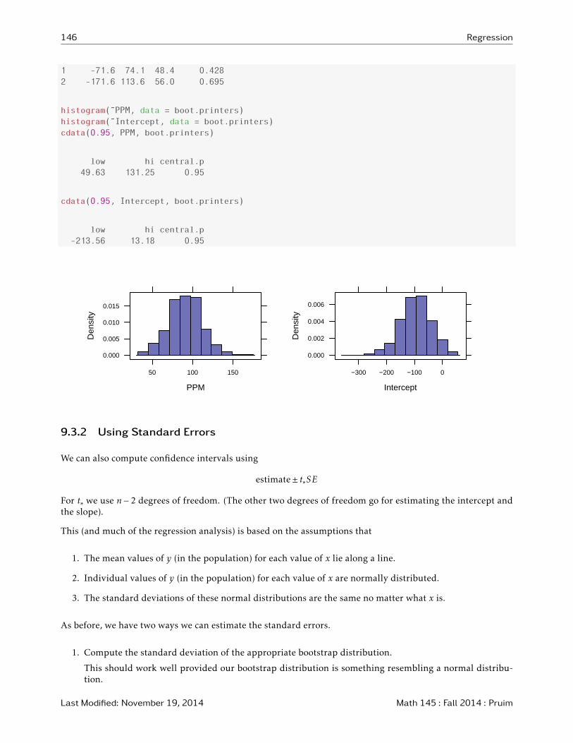
1 -71.6 74.1 48.4 0.428

2 -171.6 113.6 56.0 0.695

histogram(˜PPM, data = boot.printers)

histogram(˜Intercept, data = boot.printers)

cdata(0.95, PPM, boot.printers)

low hi central.p

49.63 131.25 0.95

cdata(0.95, Intercept, boot.printers)

low hi central.p

-213.56 13.18 0.95

PPM

Den

sity

0.000

0.005

0.010

0.015

50 100 150

Intercept

Den

sity

0.000

0.002

0.004

0.006

−300 −200 −100 0

9.3.2 Using Standard Errors

We can also compute confidence intervals using

estimate± t∗SE

For t∗ we use n− 2 degrees of freedom. (The other two degrees of freedom go for estimating the intercept andthe slope).

This (and much of the regression analysis) is based on the assumptions that

1. The mean values of y (in the population) for each value of x lie along a line.

2. Individual values of y (in the population) for each value of x are normally distributed.

3. The standard deviations of these normal distributions are the same no matter what x is.

As before, we have two ways we can estimate the standard errors.

1. Compute the standard deviation of the appropriate bootstrap distribution.

This should work well provided our bootstrap distribution is something resembling a normal distribu-tion.


Regression 147

2. Use formulas to compute the standard errors from summary statistics.

The formulas for SE are a bit more complicated in this case, but R will standard error estimates for us,so we don’t need to know the formulas.

Florida Lakes

The t∗ value is based on DFE, the degrees of freedom for the errors (residuals). For simple linear regression,the error degrees of freedom is n− 2 = 51. For a 95% confidence interval, we first compute t∗:

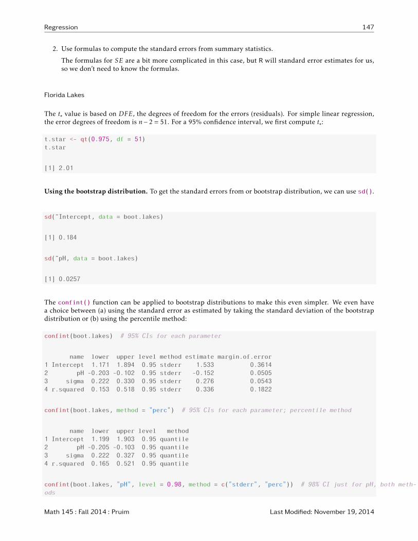
t.star <- qt(0.975, df = 51)

t.star

[1] 2.01

Using the bootstrap distribution. To get the standard errors from or bootstrap distribution, we can use sd().

sd(˜Intercept, data = boot.lakes)

[1] 0.184

sd(˜pH, data = boot.lakes)

[1] 0.0257

The confint() function can be applied to bootstrap distributions to make this even simpler. We even havea choice between (a) using the standard error as estimated by taking the standard deviation of the bootstrapdistribution or (b) using the percentile method:

confint(boot.lakes) # 95% CIs for each parameter

name lower upper level method estimate margin.of.error

1 Intercept 1.171 1.894 0.95 stderr 1.533 0.3614

2 pH -0.203 -0.102 0.95 stderr -0.152 0.0505

3 sigma 0.222 0.330 0.95 stderr 0.276 0.0543

4 r.squared 0.153 0.518 0.95 stderr 0.336 0.1822

confint(boot.lakes, method = "perc") # 95% CIs for each parameter; percentile method

name lower upper level method

1 Intercept 1.199 1.903 0.95 quantile

2 pH -0.205 -0.103 0.95 quantile

3 sigma 0.222 0.327 0.95 quantile

4 r.squared 0.165 0.521 0.95 quantile

confint(boot.lakes, "pH", level = 0.98, method = c("stderr", "perc")) # 98% CI just for pH, both meth-

ods


148 Regression


1 pH -0.212 -0.0924 0.98 stderr -0.152 0.06

2 pH -0.221 -0.0980 0.98 quantile NA NA

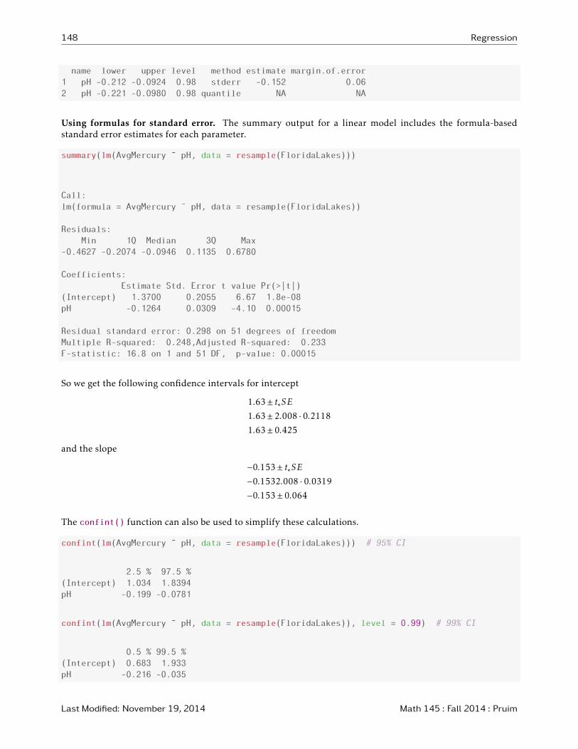
Using formulas for standard error. The summary output for a linear model includes the formula-basedstandard error estimates for each parameter.

summary(lm(AvgMercury ˜ pH, data = resample(FloridaLakes)))

Call:

lm(formula = AvgMercury ˜ pH, data = resample(FloridaLakes))

Residuals:


-0.4627 -0.2074 -0.0946 0.1135 0.6780

Coefficients:


(Intercept) 1.3700 0.2055 6.67 1.8e-08

pH -0.1264 0.0309 -4.10 0.00015



F-statistic: 16.8 on 1 and 51 DF, p-value: 0.00015

So we get the following confidence intervals for intercept

1.63± t∗SE

1.63± 2.008 · 0.2118

1.63± 0.425

and the slope

−0.153± t∗SE

−0.1532.008 · 0.0319

−0.153± 0.064

The confint() function can also be used to simplify these calculations.

confint(lm(AvgMercury ˜ pH, data = resample(FloridaLakes))) # 95% CI

2.5 % 97.5 %

(Intercept) 1.034 1.8394

pH -0.199 -0.0781

confint(lm(AvgMercury ˜ pH, data = resample(FloridaLakes)), level = 0.99) # 99% CI

0.5 % 99.5 %

(Intercept) 0.683 1.933

pH -0.216 -0.035


Regression 149

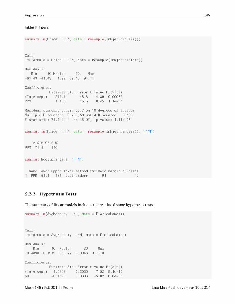
Inkjet Printers

summary(lm(Price ˜ PPM, data = resample(InkjetPrinters)))

Call:

lm(formula = Price ˜ PPM, data = resample(InkjetPrinters))

Residuals:


-61.43 -41.43 1.99 29.15 94.44

Coefficients:


(Intercept) -214.1 48.8 -4.39 0.00035

PPM 131.3 15.5 8.45 1.1e-07




confint(lm(Price ˜ PPM, data = resample(InkjetPrinters)), "PPM")

2.5 % 97.5 %

PPM 71.4 140

confint(boot.printers, "PPM")


1 PPM 51.1 131 0.95 stderr 91 40

9.3.3 Hypothesis Tests

The summary of linear models includes the results of some hypothesis tests:

summary(lm(AvgMercury ˜ pH, data = FloridaLakes))

Call:


Residuals:


-0.4890 -0.1919 -0.0577 0.0946 0.7113

Coefficients:


(Intercept) 1.5309 0.2035 7.52 8.1e-10

pH -0.1523 0.0303 -5.02 6.6e-06


150 Regression




Of these the most interesting is the one in the row labeled pH. This is a test of

• H0 : β1 = 0

• Ha : β1 , 0

The test statistic t =β1−0SE is converted to a p-value using a t-distribution with DFE = n− 2 degrees of freedom.

t <- -0.1523 / 0.0303; t

[1] -5.03

2 * pt( t, df = 51 ) # p-value

[1] 6.52e-06

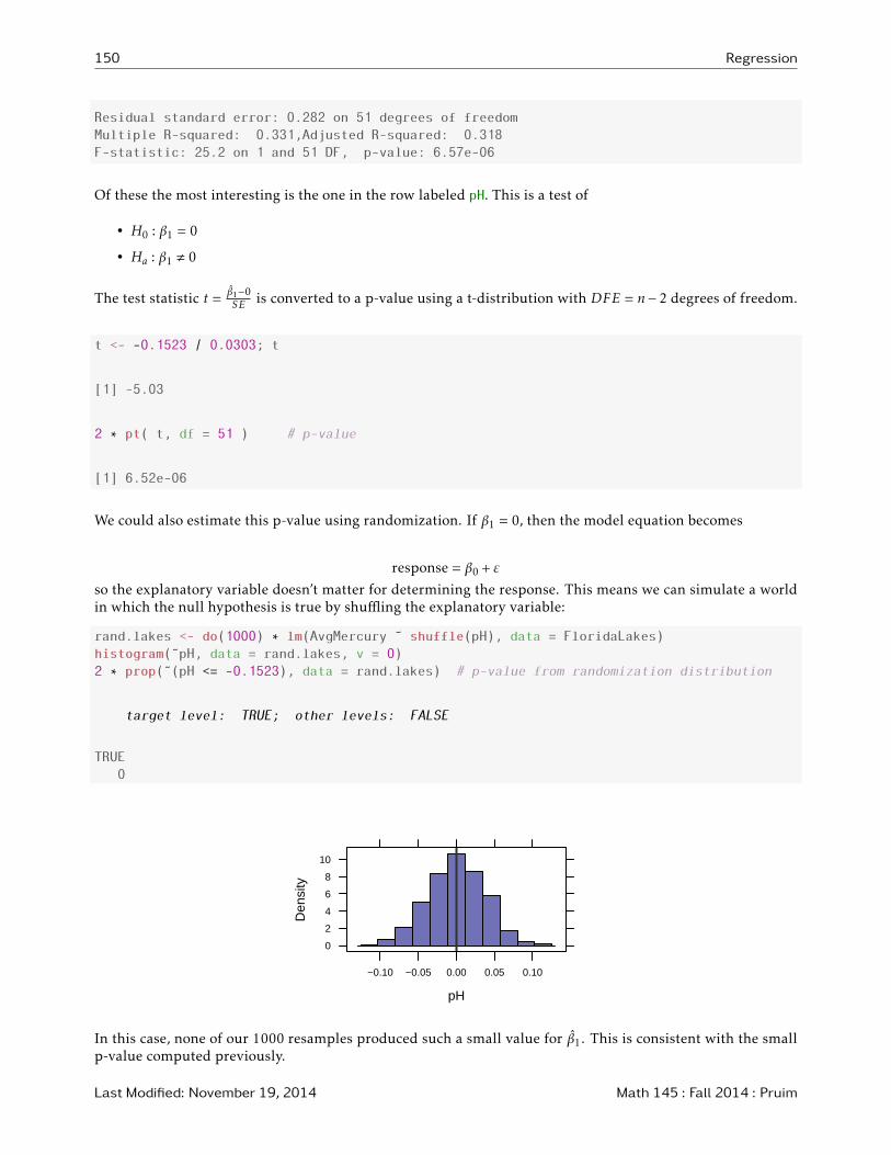
We could also estimate this p-value using randomization. If β1 = 0, then the model equation becomes

response = β0 + ε

so the explanatory variable doesn’t matter for determining the response. This means we can simulate a worldin which the null hypothesis is true by shuffling the explanatory variable:

rand.lakes <- do(1000) * lm(AvgMercury ˜ shuffle(pH), data = FloridaLakes)

histogram(˜pH, data = rand.lakes, v = 0)

2 * prop(˜(pH <= -0.1523), data = rand.lakes) # p-value from randomization distribution

target level: TRUE; other levels: FALSE

TRUE

0

pH

Den

sity

0

2

4

6

8

10

−0.10 −0.05 0.00 0.05 0.10

In this case, none of our 1000 resamples produced such a small value for β1. This is consistent with the smallp-value computed previously.


Regression 151

9.4 Making Predictions

9.4.1 Point Estimates for Response

It may be very interesting to make predictions when the explanatory variable has some other value, however.There are two ways to do this in R. One uses the predict() function. It is simpler, however, to use themakeFun() function in the mosaic package, so that’s the approach we will use here.

First, let’s build our linear model and store it.

lakes.model <- lm(AvgMercury ˜ pH, data = FloridaLakes)

coef(lakes.model)

(Intercept) pH

1.531 -0.152

Now let’s create a function that will estimate values of AvgMercury for a given value of pH:

mercury <- makeFun(lakes.model)

We can now input a pH value and see what our least squares regression line predicts for the average mercurylevel in the fish:

mercury(pH = 5) # estimate AvgMercury when pH is 5

1

0.769

mercury(pH = 7) # estimate AvgMercury when pH is 5

1

0.465

9.4.2 Interval Estimates for the Mean and Individual Response

R can compute two kinds of confidence intervals for the response for a given value

1. A confidence interval for the mean response for a given explanatory value can be computed by addinginterval='confidence'.

mercury(pH = 5, interval = "confidence")

fit lwr upr

1 0.769 0.645 0.894

2. An interval for an individual response (called a prediction interval to avoid confusion with the confidenceinterval above) can be computed by adding interval='prediction' instead.


152 Regression

mercury(pH = 5, interval = "prediction")

fit lwr upr

1 0.769 0.191 1.35

Prediction intervals

(a) are much wider than confidence intervals

(b) are very sensitive to the assumption that the population normal for each value of the predictor.

(c) are (for a 95% confidence level) a little bit wider than

y ± 2SE

where SE is the “residual standard error” reported in the summary output.

The prediction interval is a little wider because it takes into account the uncertainty in ourestimated slope and intercept as well as the variability of responses around the true regressionline.

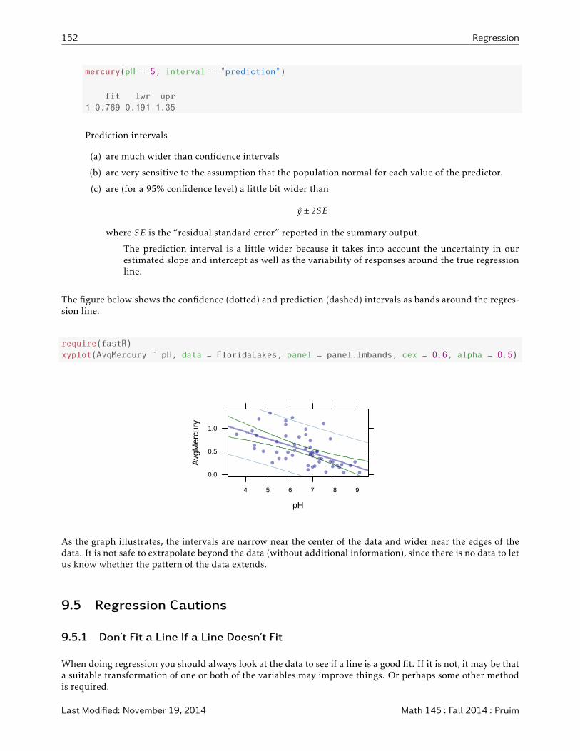
The figure below shows the confidence (dotted) and prediction (dashed) intervals as bands around the regres-sion line.

require(fastR)

xyplot(AvgMercury ˜ pH, data = FloridaLakes, panel = panel.lmbands, cex = 0.6, alpha = 0.5)

pH

Avg

Mer

cury

0.0

0.5

1.0

4 5 6 7 8 9

As the graph illustrates, the intervals are narrow near the center of the data and wider near the edges of thedata. It is not safe to extrapolate beyond the data (without additional information), since there is no data to letus know whether the pattern of the data extends.

9.5 Regression Cautions

9.5.1 Don’t Fit a Line If a Line Doesn’t Fit

When doing regression you should always look at the data to see if a line is a good fit. If it is not, it may be thata suitable transformation of one or both of the variables may improve things. Or perhaps some other methodis required.


Regression 153

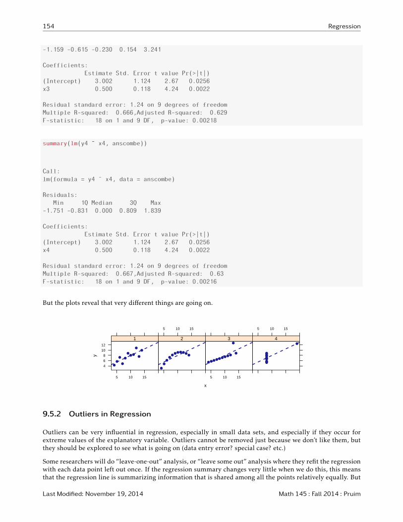
Anscombe’s Data

Anscombe illustrated the importance of looking at the data by concocting an interesting data set.

Notice how similar the numerical summaries are for these for pairs of variables

summary(lm(y1 ˜ x1, anscombe))

Call:

lm(formula = y1 ˜ x1, data = anscombe)

Residuals:


-1.9213 -0.4558 -0.0414 0.7094 1.8388

Coefficients:


(Intercept) 3.000 1.125 2.67 0.0257

x1 0.500 0.118 4.24 0.0022



F-statistic: 18 on 1 and 9 DF, p-value: 0.00217


Call:


Residuals:


-1.901 -0.761 0.129 0.949 1.269

Coefficients:


(Intercept) 3.001 1.125 2.67 0.0258

x2 0.500 0.118 4.24 0.0022





Call:


Residuals:



154 Regression

-1.159 -0.615 -0.230 0.154 3.241

Coefficients:


(Intercept) 3.002 1.124 2.67 0.0256

x3 0.500 0.118 4.24 0.0022





Call:


Residuals:


-1.751 -0.831 0.000 0.809 1.839

Coefficients:


(Intercept) 3.002 1.124 2.67 0.0256

x4 0.500 0.118 4.24 0.0022




But the plots reveal that very different things are going on.

x

y

4

6

8

10

12

5 10 15

●● ●

● ●

●

●

●

●

●●

1

5 10 15

●● ●● ●

●

●

●

●

●

●

2

5 10 15

●●

●

●●

●

●●

●

●●

3

5 10 15

●●

●●●●

●

●

●

●●

4

9.5.2 Outliers in Regression

Outliers can be very influential in regression, especially in small data sets, and especially if they occur forextreme values of the explanatory variable. Outliers cannot be removed just because we don’t like them, butthey should be explored to see what is going on (data entry error? special case? etc.)

Some researchers will do “leave-one-out” analysis, or “leave some out” analysis where they refit the regressionwith each data point left out once. If the regression summary changes very little when we do this, this meansthat the regression line is summarizing information that is shared among all the points relatively equally. But


Regression 155

if removing one or a small number of values makes a dramatic change, then we know that that point is exertinga lot of influence over the resulting analysis (a cause for caution).

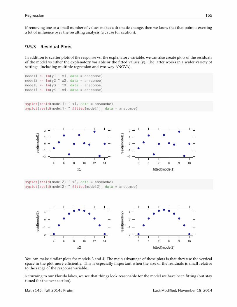
9.5.3 Residual Plots

In addition to scatter plots of the response vs. the explanatory variable, we can also create plots of the residualsof the model vs either the explanatory variable or the fitted values (y). The latter works in a wider variety ofsettings (including multiple regression and two-way ANOVA).

model1 <- lm(y1 ˜ x1, data = anscombe)




xyplot(resid(model1) ˜ x1, data = anscombe)

xyplot(resid(model1) ˜ fitted(model1), data = anscombe)

x1

resi

d(m

odel

1)

−2

−1

0

1

2

4 6 8 10 12 14

●●

●

●

● ●

●

●

●

●

●

fitted(model1)

resi

d(m

odel

1)

−2

−1

0

1

2

5 6 7 8 9 10

●●

●

●

● ●

●

●

●

●

●

xyplot(resid(model2) ˜ x2, data = anscombe)

xyplot(resid(model2) ˜ fitted(model2), data = anscombe)

x2

resi

d(m

odel

2)

−2

−1

0

1

4 6 8 10 12 14

●●

●

●

●

●

●

●

●

●

●

fitted(model2)

resi

d(m

odel

2)

−2

−1

0

1

5 6 7 8 9 10

●●

●

●

●

●

●

●

●

●

●

You can make similar plots for models 3 and 4. The main advantage of these plots is that they use the verticalspace in the plot more efficiently. This is especially important when the size of the residuals is small relativeto the range of the response variable.

Returning to our Florida lakes, we see that things look reasonable for the model we have been fitting (but staytuned for the next section).


156 Regression

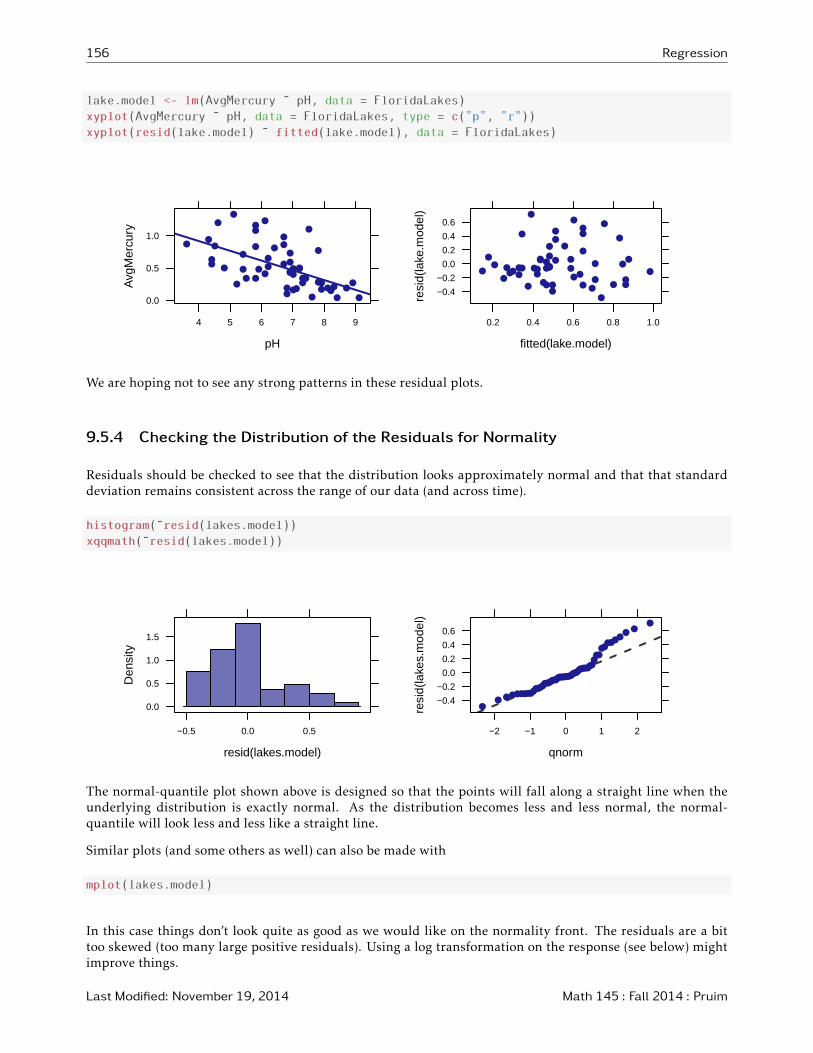
lake.model <- lm(AvgMercury ˜ pH, data = FloridaLakes)

xyplot(AvgMercury ˜ pH, data = FloridaLakes, type = c("p", "r"))

xyplot(resid(lake.model) ˜ fitted(lake.model), data = FloridaLakes)

pH

Avg

Mer

cury

0.0

0.5

1.0

4 5 6 7 8 9

●●

●

●

●

●

●

●

● ●●

●●

●

●● ●

●

●●

●●

●

●

●

●

●

●

●● ●●

●

●

●●●●

●

●

●●

●

●

●

●●

●

●

●●

● ●

fitted(lake.model)

resi

d(la

ke.m

odel

)

−0.4

−0.2

0.0

0.2

0.4

0.6

0.2 0.4 0.6 0.8 1.0

● ●

●●

●

●●

●

●●

●●●

●

●

●●

● ●●

●

●

●

●

●

●

●●

●●

● ● ●

●●

● ●●

●

●

●●

●●

●

●●● ●

●●

●

●

We are hoping not to see any strong patterns in these residual plots.

9.5.4 Checking the Distribution of the Residuals for Normality

Residuals should be checked to see that the distribution looks approximately normal and that that standarddeviation remains consistent across the range of our data (and across time).

histogram(˜resid(lakes.model))

xqqmath(˜resid(lakes.model))

resid(lakes.model)

Den

sity

0.0

0.5

1.0

1.5

−0.5 0.0 0.5

qnorm

resi

d(la

kes.

mod

el)

−0.4

−0.2

0.0

0.2

0.4

0.6

−2 −1 0 1 2

●● ●●●●●●●●

●●●●●●●●●●●

●●●●●●●●●●●●●

●●●●●●●●●●

●●●●●●

● ●●

The normal-quantile plot shown above is designed so that the points will fall along a straight line when theunderlying distribution is exactly normal. As the distribution becomes less and less normal, the normal-quantile will look less and less like a straight line.

Similar plots (and some others as well) can also be made with

mplot(lakes.model)

In this case things don’t look quite as good as we would like on the normality front. The residuals are a bittoo skewed (too many large positive residuals). Using a log transformation on the response (see below) mightimprove things.


Regression 157

9.5.5 Tranformations

Transformations of one or both variables can change the shape of the relationship (from non-linear to linear,we hope) and also the distribution of the residuals. In biological applications, a logarithmic transformation isoften useful.

lakes.model2 <- lm(log(AvgMercury) ˜ pH, data = FloridaLakes)

xyplot(log(AvgMercury) ˜ pH, data = FloridaLakes, type = c("p", "r"))

summary(lakes.model2)

Call:

lm(formula = log(AvgMercury) ˜ pH, data = FloridaLakes)

Residuals:


-1.6794 -0.4315 0.0994 0.4422 1.3715

Coefficients:


(Intercept) 1.7400 0.4819 3.61 7e-04

pH -0.4022 0.0718 -5.60 8.5e-07




pH

log(

Avg

Mer

cury

)

−3

−2

−1

0

4 5 6 7 8 9

●●

●

●

●

●

●

●

● ●●●●

●

●

●●

●● ●

● ●●

●

●

●

●

●

●●

●●

●●

●●●

●

●

●

●

●

●

●

●

●●

●

●

●●

● ●

If we like, we can show the new model fit overlaid on the original data:

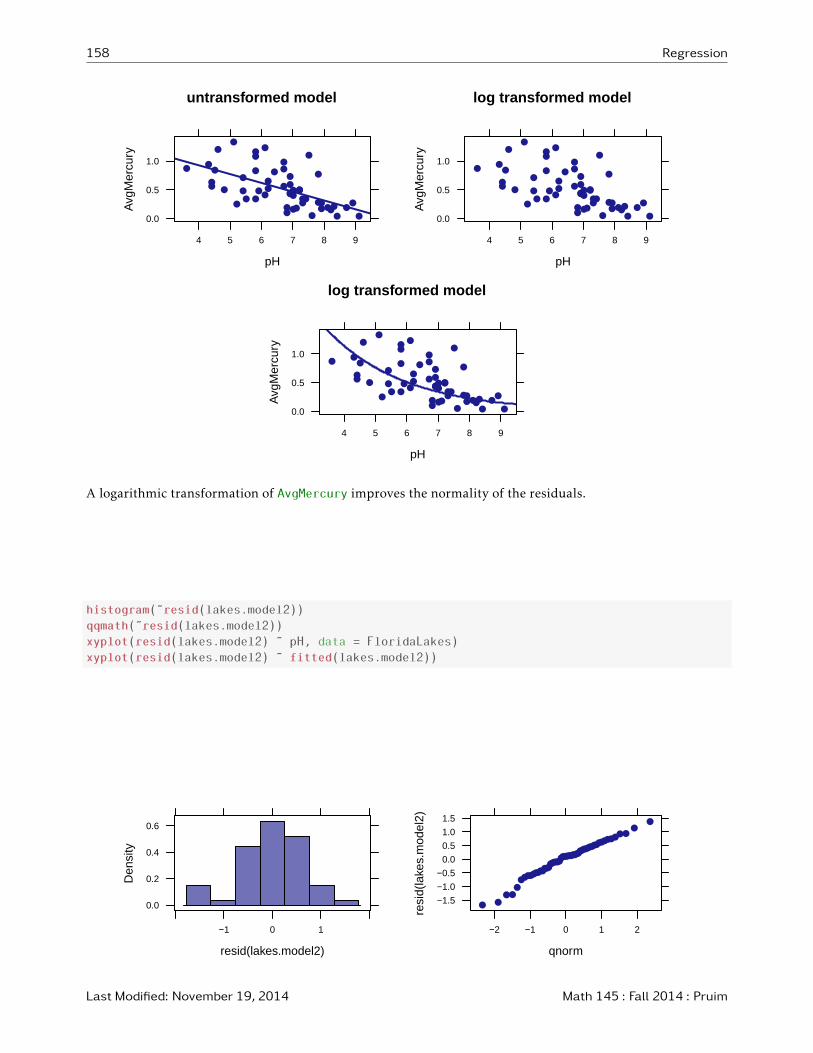
xyplot(AvgMercury ˜ pH, data = FloridaLakes, main = "untransformed model", type = c("p", "r"))

xyplot(AvgMercury ˜ pH, data = FloridaLakes, main = "log transformed model")

Hg <- makeFun(lakes.model2) # turn model into a function

plotFun(exp(Hg(pH)) ˜ pH, add = TRUE) # add this function to the plot


158 Regression

untransformed model

pH

Avg

Mer

cury

0.0

0.5

1.0

4 5 6 7 8 9

●●

●

●

●

●

●

●

● ●●

●●

●

●● ●

●

●●

● ●●

●

●

●

●

●

●● ●●

●

●

●●●●

●

●

●●

●

●

●

●●

●

●

●●● ●

log transformed model

pH

Avg

Mer

cury

0.0

0.5

1.0

4 5 6 7 8 9

●●

●

●

●

●

●

●

● ●●

●●

●

●● ●

●

●●

● ●●

●

●

●

●

●

●● ●●

●

●

●●●●

●

●

●●

●

●

●

●●

●

●

●●● ●

log transformed model

pH

Avg

Mer

cury

0.0

0.5

1.0

4 5 6 7 8 9

●●

●

●

●

●

●

●

● ●●

●●

●

●● ●

●

●●

● ●●

●

●

●

●

●

●● ●●

●

●

●●●●

●

●

●●

●

●

●

●●

●

●

●●● ●

A logarithmic transformation of AvgMercury improves the normality of the residuals.

histogram(˜resid(lakes.model2))

qqmath(˜resid(lakes.model2))

xyplot(resid(lakes.model2) ˜ pH, data = FloridaLakes)

xyplot(resid(lakes.model2) ˜ fitted(lakes.model2))

resid(lakes.model2)

Den

sity

0.0

0.2

0.4

0.6

−1 0 1

qnorm

resi

d(la

kes.

mod

el2)

−1.5

−1.0

−0.5

0.0

0.5

1.0

1.5

−2 −1 0 1 2

● ●●●

●●●●

●●●●●●●●●

●●●●●●●●●●●●●●●●

●●●●●●●●●●

●●●●●●●●

●●


Regression 159

pH

resi

d(la

kes.

mod

el2)

−1.5

−1.0

−0.5

0.0

0.5

1.0

1.5

4 5 6 7 8 9

●●

●

●●

●●

●

●●

●●●

●

●

●

●

●

●●

●

●

●

●

●

●

●●

● ●

●●

● ●●

●●

●

●

●

●

●

● ●

●

●●

●

●●●

●

●

fitted(lakes.model2)

resi

d(la

kes.

mod

el2)

−1.5

−1.0

−0.5

0.0

0.5

1.0

1.5

−2.0 −1.5 −1.0 −0.5 0.0

●●

●

● ●

●●

●

●●

●●●

●

●

●

●

●

●●

●

●

●

●

●

●

●●

●●

● ●

●●●

● ●

●

●

●

●

●

●●

●

●●

●

●●●

●

●

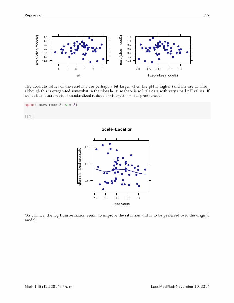
The absolute values of the residuals are perhaps a bit larger when the pH is higher (and fits are smaller),although this is exagerated somewhat in the plots because there is so little data with very small pH values. Ifwe look at square roots of standardized residuals this effect is not as pronounced:

mplot(lakes.model2, w = 3)

[[1]]

Scale−Location

Fitted Value

Sta

ndar

dize

d re

sidu

als

0.5

1.0

1.5

−2.0 −1.5 −1.0 −0.5 0.0

●

●

●

●

●

●

●

●

●

●

●

●●

●

●

●

●

●

●

●

●●

●

●●

●

● ●

●●

●●

●

●

●

●●

●

●

●

●

●

●

●

●

●

●

●

●

●●

●

●

On balance, the log transformation seems to improve the situation and is to be preferred over the originalmodel.


Documents

Regression 9.1 Simple Linear Regression - Calvin Collegerpruim/courses/m145/F14/Notes/Regression.pdf · Estimate the slope and intercept of your line by reading them oﬀof the graph