Correlation and Regression: Example - The Personality Projectpersonality-project.org/revelle/syllabi/405/regression.pdf · Preliminaries Simple regressions Multiple R with interaction

Preliminaries Simple regressions Multiple R with interaction terms Using mat.regress or set.cor

Correlation and Regression: Example

405: Psychometric Theory

Department of PsychologyNorthwestern UniversityEvanston, Illinois USA

April, 2012


Outline

1 PreliminariesGetting the data and describing itTransforming the data

2 Simple regressionsUsing the raw dataUsing transformed dataMultiple regression

3 Multiple R with interaction termsPlotting interactions and regressions

4 Using mat.regress or set.corSummaries of three multiple regressions


Use R


Getting the data and describing it

Get the data

A nice feature of R is that you can read from remote data sets.The example dataset is on the personality-project.org server. Get itand describe it.> da t a f i l e n ame=”ht tp : // p e r s o n a l i t y−p r o j e c t . o rg /R/ d a t a s e t s / p s y chome t r i c s . prob2 . t x t ”> mydata =read . t a b l e ( da t a f i l e name , heade r=TRUE) #read the data file> d e s c r i b e (mydata , skew=FALSE)

v a r n mean sd median trimmed mad min max range seID 1 1000 500 .50 288 .82 500 .50 500 .50 370 .65 1 . 0 1000.00 999 .00 9 . 1 3GREV 2 1000 499 .77 106 .11 497 .50 498 .75 106 .01 1 3 8 . 0 873 .00 735 .00 3 . 3 6GREQ 3 1000 500 .53 103 .85 498 .00 498 .51 105 .26 1 9 1 . 0 914 .00 723 .00 3 . 2 8GREA 4 1000 498 .13 100 .45 495 .00 498 .67 9 9 . 3 3 2 0 7 . 0 848 .00 641 .00 3 . 1 8Ach 5 1000 4 9 . 9 3 9 . 8 4 5 0 . 0 0 4 9 . 8 8 1 0 . 3 8 1 6 . 0 7 9 . 0 0 6 3 . 0 0 0 . 3 1Anx 6 1000 5 0 . 3 2 9 . 9 1 5 0 . 0 0 5 0 . 4 3 1 0 . 3 8 1 4 . 0 7 8 . 0 0 6 4 . 0 0 0 . 3 1P r e l i m 7 1000 1 0 . 0 3 1 . 0 6 1 0 . 0 0 1 0 . 0 2 1 . 4 8 7 . 0 1 3 . 0 0 6 . 0 0 0 . 0 3GPA 8 1000 4 . 0 0 0 . 5 0 4 . 0 2 4 . 0 1 0 . 5 3 2 . 5 5 . 3 8 2 . 8 8 0 . 0 2MA 9 1000 3 . 0 0 0 . 4 9 3 . 0 0 3 . 0 0 0 . 4 4 1 . 4 4 . 5 0 3 . 1 0 0 . 0 2



Plot it

Use the pairs.panels function to show a splom plot (use gap=0 and pch=’.’).

>pairs.panels(mydata,pch=”.”,gap=0) #pch=’.’ makes for a cleaner plot

ID

200 600

-0.01 0.00

200 500 800

-0.01 0.00

20 50 80

-0.01 0.02

2.5 4.0

0.00

0400

1000

-0.01

200

600 GREV

0.73 0.64 0.01 0.01 0.43 0.42 0.32GREQ

0.60 0.01 0.01 0.38 0.37

200

6000.29

200500800

GREA0.45 -0.39 0.57 0.52 0.45Ach

-0.56 0.30 0.28

2050

80

0.26

2050

80 Anx-0.23 -0.22 -0.22

Prelim0.42

79

110.36

2.5

4.0

GPA0.31

0 400 1000 200 600 20 50 80 7 9 11 1.5 3.0 4.5

1.5

3.0

4.5

MA



Plot it

Use the pairs.panels function to show a splom plot. Select a subsetof variables using the c() function.>pairs.panels(mydata[c(2:4,6:8)],pch=’.’)

GREV

200 600

0.73 0.64

20 40 60 80

0.01 0.43

2.5 3.5 4.5

200

600

0.42

200

600

GREQ0.60 0.01 0.38 0.37

GREA-0.39 0.57

200

500

800

0.52

2040

6080

Anx-0.23 -0.22

Prelim

79

1113

0.42

200 600

2.5

3.5

4.5

200 500 800 7 9 11 13

GPA



Do this for the first 200 subjects

> pairs.panels(mydata[mydata$ID < 200,c(2:4,6:8)])

GREV

300 500 700

0.78 0.67

30 50 70

-0.06 0.45

3.0 4.0 5.0

300

500

700

0.51

300500700 GREQ

0.62 -0.05 0.44 0.44

GREA-0.41 0.52

200400600800

0.54

3050

70 Anx-0.19 -0.23

Prelim7

911

13

0.40

300 500 700

3.0

4.0

5.0

200 400 600 800 7 9 11 13

GPA


Transforming the data

0 center the data

In order to do interaction terms in regressions, it is necessary to 0center the data. We need to turn the result into a data.frame inorder to use it in the regression function.

> cent <− data . frame ( s c a l e (mydata , s c a l e=FALSE ) )> d e s c r i b e ( cent , skew=FALSE)

v a r n mean sd median trimmed mad min max range seID 1 1000 0 288 .82 0 . 0 0 0 . 0 0 370 .65 −499.50 499 .50 999 .00 9 . 1 3GREV 2 1000 0 106.11 −2.27 −1.02 106 .01 −361.77 373 .23 735 .00 3 . 3 6GREQ 3 1000 0 103.85 −2.53 −2.02 105 .26 −309.53 413 .47 723 .00 3 . 2 8GREA 4 1000 0 100.45 −3.13 0 . 5 4 9 9 . 3 3 −291.13 349 .87 641 .00 3 . 1 8Ach 5 1000 0 9 . 8 4 0 . 0 7 −0.05 1 0 . 3 8 −33.93 2 9 . 0 7 6 3 . 0 0 0 . 3 1Anx 6 1000 0 9 . 9 1 −0.32 0 . 1 1 1 0 . 3 8 −36.32 2 7 . 6 8 6 4 . 0 0 0 . 3 1P r e l i m 7 1000 0 1 . 0 6 −0.03 0 . 0 0 1 . 4 8 −3.03 2 . 9 7 6 . 0 0 0 . 0 3GPA 8 1000 0 0 . 5 0 0 . 0 2 0 . 0 0 0 . 5 3 −1.50 1 . 3 8 2 . 8 8 0 . 0 2MA 9 1000 0 0 . 4 9 0 . 0 0 0 . 0 0 0 . 4 4 −1.60 1 . 5 0 3 . 1 0 0 . 0 2


Transforming the data

The standardized data

Alternatively, we could standardize it.

> z . data <− data . frame ( s c a l e (my . data ) )> d e s c r i b e ( z . data )

v a r n mean sd median trimmed mad min max range skew k u r t o s i s seID 1 1000 0 1 0 . 0 0 0 . 0 0 1 . 2 8 −1.73 1 . 7 3 3 . 4 6 0 . 0 0 −1.20 0 . 0 3GREV 2 1000 0 1 −0.02 −0.01 1 . 0 0 −3.41 3 . 5 2 6 . 9 3 0 . 0 9 −0.07 0 . 0 3GREQ 3 1000 0 1 −0.02 −0.02 1 . 0 1 −2.98 3 . 9 8 6 . 9 6 0 . 2 2 0 . 0 8 0 . 0 3GREA 4 1000 0 1 −0.03 0 . 0 1 0 . 9 9 −2.90 3 . 4 8 6 . 3 8 −0.02 −0.06 0 . 0 3Ach 5 1000 0 1 0 . 0 1 −0.01 1 . 0 5 −3.45 2 . 9 5 6 . 4 0 0 . 0 0 0 . 0 2 0 . 0 3Anx 6 1000 0 1 −0.03 0 . 0 1 1 . 0 5 −3.67 2 . 7 9 6 . 4 6 −0.14 0 . 1 4 0 . 0 3P r e l i m 7 1000 0 1 −0.02 0 . 0 0 1 . 4 0 −2.86 2 . 8 1 5 . 6 7 −0.02 −0.01 0 . 0 3GPA 8 1000 0 1 0 . 0 3 0 . 0 1 1 . 0 6 −3.00 2 . 7 4 5 . 7 4 −0.07 −0.29 0 . 0 3MA 9 1000 0 1 0 . 0 1 0 . 0 1 0 . 9 0 −3.23 3 . 0 4 6 . 2 7 −0.07 −0.09 0 . 0 3


Using the raw data

Find the regression of rated Prelim score on GREV

> mod1 <− lm (GPA˜GREV, data=mydata )> summary ( mod1 )

C a l l :lm ( fo rmula = GPA ˜ GREV, data = mydata )

R e s i d u a l s :Min 1Q Median 3Q Max

−1.45807 −0.32322 0.00107 0.32811 1.44850

C o e f f i c i e n t s :E s t i m a t e Std . E r r o r t v a l u e Pr (>| t | )

( I n t e r c e p t ) 3 .0117292 0.0694343 4 3 . 3 8 <2e−16 ∗∗∗GREV 0.0019839 0.0001359 1 4 . 6 0 <2e−16 ∗∗∗−−−S i g n i f . codes : 0 O∗∗∗O 0 . 0 0 1 O∗∗O 0 . 0 1 O∗O 0 . 0 5 O.O 0 . 1 O O 1

R e s i d u a l s t a n d a r d e r r o r : 0 .4558 on 998 d e g r e e s o f f reedomM u l t i p l e R−s q u a r e d : 0 . 1 7 6 , A d j u s t e d R−s q u a r e d : 0 .1751F− s t a t i s t i c : 2 1 3 . 1 on 1 and 998 DF, p−v a l u e : < 2 . 2 e−16


Using transformed data

Regression on z transformed data

> mod2 <− lm (GPA˜GREV, data=z . data )> summary ( mod2 )

C a l l :lm ( fo rmula = GPA ˜ GREV, data = z . data )


−2.90526 −0.64404 0.00213 0.65377 2.88619


( I n t e r c e p t ) 1 . 8 8 8 e−17 2 . 8 7 2 e−02 0 . 0 0 1GREV 4 . 1 9 5 e−01 2 . 8 7 3 e−02 1 4 . 6 0 <2e−16 ∗∗∗−−−S i g n i f . codes : 0 O∗∗∗O 0 . 0 0 1 O∗∗O 0 . 0 1 O∗O 0 . 0 5 O.O 0 . 1 O O 1


Note that the slope is the same as the correlation.


Using transformed data

> mod3 <− lm (GPA˜GREV, data=c e n t )> summary ( mod3 )

C a l l :lm ( fo rmula = GPA ˜ GREV, data = c e n t )


−1.45807 −0.32322 0.00107 0.32811 1.44850


( I n t e r c e p t ) −3.332 e−17 1 . 4 4 1 e−02 0 . 0 0 1GREV 1 . 9 8 4 e−03 1 . 3 5 9 e−04 1 4 . 6 0 <2e−16 ∗∗∗−−−S i g n i f . codes : 0 O∗∗∗O 0 . 0 0 1 O∗∗O 0 . 0 1 O∗O 0 . 0 5 O.O 0 . 1 O O 1


Note that the slope of the centered data is in the same units as theraw data, just the intercept has changed.


Multiple regression

2 predictors

> summary ( lm (GPA ˜ GREV + GREQ , data= c e n t ) )

C a l l :lm ( fo rmula = GPA ˜ GREV + GREQ, data = c e n t )


−1.42442 −0.33228 0.00616 0.32465 1.43765


( I n t e r c e p t ) −2.651 e−17 1 . 4 3 5 e−02 0 . 0 0 0 1.00000GREV 1 . 5 3 4 e−03 1 . 9 7 6 e−04 7 . 7 6 0 2 . 1 0 e−14 ∗∗∗GREQ 6 . 3 1 4 e−04 2 . 0 1 9 e−04 3 . 1 2 7 0.00182 ∗∗−−−S i g n i f . codes : 0 O∗∗∗O 0 . 0 0 1 O∗∗O 0 . 0 1 O∗O 0 . 0 5 O.O 0 . 1 O O 1



Multiple regression

Multiple R with z transformed data

Do the same regression, but on the z transformed data. The unitsare now in correlation units.> z . data <− data . frame ( s c a l e (my . data ) )> summary ( lm (GPA ˜ GREV + GREQ , data= z . data ) )

C a l l :lm ( fo rmula = GPA ˜ GREV + GREQ, data = z . data )


−2.83821 −0.66208 0.01228 0.64688 2.86457


( I n t e r c e p t ) 3 . 2 0 5 e−17 2 . 8 6 0 e−02 0 . 0 0 0 1.00000GREV 3 . 2 4 2 e−01 4 . 1 7 9 e−02 7 . 7 6 0 2 . 1 0 e−14 ∗∗∗GREQ 1 . 3 0 6 e−01 4 . 1 7 9 e−02 3 . 1 2 7 0.00182 ∗∗−−−S i g n i f . codes : 0 O∗∗∗O 0 . 0 0 1 O∗∗O 0 . 0 1 O∗O 0 . 0 5 O.O 0 . 1 O O 1



Multiple regression

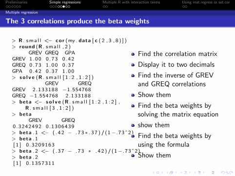
The 3 correlations produce the beta weights

> R . s m a l l <− cor (my . data [ c ( 2 , 3 , 8 ) ] )> round (R . s m a l l , 2 )

GREV GREQ GPAGREV 1 . 0 0 0 . 7 3 0 . 4 2GREQ 0 . 7 3 1 . 0 0 0 . 3 7GPA 0 . 4 2 0 . 3 7 1 . 0 0> s o l v e (R . s m a l l [ 1 : 2 , 1 : 2 ] )

GREV GREQGREV 2.133188 −1.554768GREQ −1.554768 2.133188> beta <− s o l v e (R . s m a l l [ 1 : 2 , 1 : 2 ] ,

R . s m a l l [ 3 , 1 : 2 ] )> beta

GREV GREQ0.3242492 0.1306439> beta . 1 <− ( . 4 2 − . 7 3 ∗ . 3 7 ) / (1− .73ˆ2)> beta . 1[ 1 ] 0 .3209163> beta . 2 <− ( . 3 7 − . 7 3 ∗ . 4 2 ) / (1− .73ˆ2)> beta . 2[ 1 ] 0 .1357311

Find the correlation matrix

Display it to two decimals

Find the inverse of GREVand GREQ correlations

Show them

Find the beta weights bysolving the matrix equation

show them

Find the beta weights byusing the formula

Show them


Multiple regression

3 predictors, no interactions

Use three predictors, but print it with only 2 decimals

> p r i n t ( summary ( lm (GPA ˜ GREV + GREQ + GREA , data= c e n t ) ) , d i g i t s =3)

C a l l :lm ( fo rmula = GPA ˜ GREV + GREQ + GREA, data = c e n t )


−1.2668 −0.3038 0 .0073 0 .3051 1 .3022


( I n t e r c e p t ) −6.89e−17 1 . 3 5 e−02 0 . 0 0 1 .00000GREV 6 . 6 6 e−04 2 . 0 0 e−04 3 . 3 2 0 .00092 ∗∗∗GREQ 7 . 7 5 e−05 1 . 9 6 e−04 0 . 4 0 0 .69233GREA 2 . 0 8 e−03 1 . 8 1 e−04 1 1 . 5 2 < 2e−16 ∗∗∗−−−S i g n i f . codes : 0 O∗∗∗O 0 . 0 0 1 O∗∗O 0 . 0 1 O∗O 0 . 0 5 O.O 0 . 1 O O 1

R e s i d u a l s t a n d a r d e r r o r : 0 . 4 2 7 on 996 d e g r e e s o f f reedomM u l t i p l e R−s q u a r e d : 0 . 2 8 , A d j u s t e d R−s q u a r e d : 0 . 2 7 8F− s t a t i s t i c : 129 on 3 and 996 DF, p−v a l u e : <2e−16


Multiple regression

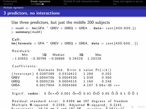
3 predictors, no interactions

Use three predictors, but just the middle 200 subjects> mod4 <− lm (GPA ˜ GREV + GREQ + GREA , data= c e n t [ 4 0 0 : 6 0 0 , ] )> summary ( mod4 )

C a l l :lm ( fo rmula = GPA ˜ GREV + GREQ + GREA, data = c e n t [ 4 0 0 : 6 0 0 , ] )


−1.03553 −0.30799 −0.00889 0.29320 1.20228


( I n t e r c e p t ) 0 .0397399 0.0310412 1 . 2 8 0 0 . 2 0 2GREV 0.0004706 0.0004530 1 . 0 3 9 0 . 3 0 0GREQ 0.0005236 0.0004515 1 . 1 6 0 0 . 2 4 8GREA 0.0017904 0.0004360 4 . 1 0 7 5 . 8 8 e−05 ∗∗∗−−−S i g n i f . codes : 0 O∗∗∗O 0 . 0 0 1 O∗∗O 0 . 0 1 O∗O 0 . 0 5 O.O 0 . 1 O O 1

R e s i d u a l s t a n d a r d e r r o r : 0 .4394 on 197 d e g r e e s o f f reedomM u l t i p l e R−s q u a r e d : 0 . 2 2 5 9 , A d j u s t e d R−s q u a r e d : 0 .2141F− s t a t i s t i c : 1 9 . 1 6 on 3 and 197 DF, p−v a l u e : 6 . 0 5 1 e−11


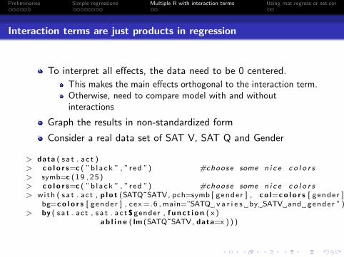
Interaction terms are just products in regression

To interpret all effects, the data need to be 0 centered.

This makes the main effects orthogonal to the interaction term.Otherwise, need to compare model with and withoutinteractions

Graph the results in non-standardized form

Consider a real data set of SAT V, SAT Q and Gender

> data ( s a t . a c t )> c o l o r s=c ( ”b l a c k ” , ”r e d ”) #choose some n i c e c o l o r s> symb=c ( 1 9 , 2 5 )> c o l o r s=c ( ”b l a c k ” , ”r e d ”) #choose some n i c e c o l o r s> w i t h ( s a t . act , p l o t (SATQ˜SATV, pch=symb [ ge n d e r ] , c o l=c o l o r s [ g e n de r ] ,

bg=c o l o r s [ g e n de r ] , cex =.6 , main=”SATQ v a r i e s by SATV and g e nd e r ”) )> by ( s a t . act , s a t . a c t $ gender , f u n c t i o n ( x )

a b l i n e ( lm (SATQ˜SATV, data=x ) ) )


Plotting interactions and regressions

An example of an interaction plot

200 300 400 500 600 700 800

200

300

400

500

600

700

800

SATQ varies by SATV and gender

SATV

SATQ

> data ( s a t . a c t )>c . s a t <− data . frame ( s c a l e ( s a t . act , s c a l e=FALSE ) )>summary ( lm (SATQ˜SATV ∗ gender , data=c . s a t ) )

C a l l :lm ( fo rmula = SATQ ˜ SATV ∗ gender , data = c . s a t )

R e s i d u a l s :Min 1Q Median

3Q Max−294.423 −49.876 5 . 5 7 7 53 .210291.100


( I n t e r c e p t ) −0.26696 3.31211−0.081 0 . 9 3 6SATV 0.65398 0.0292622 .350 < 2e−16 ∗∗∗g e nd e r −36.71820 6.91495−5.310 1 . 4 8 e−07 ∗∗∗SATV : g e nd e r −0.05835 0.06086−0.959 0 . 3 3 8−−−S i g n i f . codes :

0 O∗∗∗O 0 . 0 0 1 O∗∗O 0 . 0 1 O∗O 0 . 0 5 O.O 0 . 1 O O 1

R e s i d u a l s t a n d a r d e r r o r : 8 6 . 7 9 on 683 d e g r e e s o f f reedom(13 o b s e r v a t i o n s d e l e t e d due to m i s s i n g n e s s )

M u l t i p l e R−s q u a r e d : 0 . 4 3 9 1 , A d j u s t e d R−s q u a r e d : 0 .4367F−s t a t i s t i c : 1 7 8 . 3 on 3 and 683 DF,p−v a l u e : < 2 . 2 e−16


Plotting interactions and regressions

Interaction of Anxiety with Verbal

> mod5 <− lm (GPA ˜ GREV ∗ Anx , data=c e n t )> summary ( mod5 )

C a l l :lm ( fo rmula = GPA ˜ GREV ∗ Anx , data = c e n t )


−1.49677 −0.31527 −0.00054 0.31223 1.32156


( I n t e r c e p t ) −2.375 e−04 1 . 3 9 5 e−02 −0.017 0 . 9 8 6GREV 1 . 9 9 6 e−03 1 . 3 1 6 e−04 15 .167 < 2e−16 ∗∗∗Anx −1.131 e−02 1 . 4 1 4 e−03 −7.997 3 . 5 1 e−15 ∗∗∗GREV : Anx 2 . 2 1 9 e−05 1 . 3 7 7 e−05 1 . 6 1 2 0 . 1 0 7−−−S i g n i f . codes : 0 O∗∗∗O 0 . 0 0 1 O∗∗O 0 . 0 1 O∗O 0 . 0 5 O.O 0 . 1 O O 1

R e s i d u a l s t a n d a r d e r r o r : 0 .4412 on 996 d e g r e e s o f f reedomM u l t i p l e R−s q u a r e d : 0 . 2 2 9 4 , A d j u s t e d R−s q u a r e d : 0 . 2 2 7F− s t a t i s t i c : 9 8 . 8 1 on 3 and 996 DF, p−v a l u e : < 2 . 2 e−16


mat.regress and set.cor

set.cor (formerly mat.regress) in the psych package doesmultiple regressions (without interactions) from thecorrelation matrix.

Data can be either a correlation matrix or

Raw data

Interface is a bit cruder than lm model


Using our data set, first find the correlations. Then show the correlations to twodecimals using the lower.mat function.

> my . R <− cor ( mydata )> l ower . mat (my . R , 2 )

ID GREV GREQ GREA Ach Anx Prelm GPA MAID 1 . 0 0GREV −0.01 1 . 0 0GREQ 0 . 0 0 0 . 7 3 1 . 0 0GREA −0.01 0 . 6 4 0 . 6 0 1 . 0 0Ach 0 . 0 0 0 . 0 1 0 . 0 1 0 . 4 5 1 . 0 0Anx −0.01 0 . 0 1 0 . 0 1 −0.39 −0.56 1 . 0 0P r e l i m 0 . 0 2 0 . 4 3 0 . 3 8 0 . 5 7 0 . 3 0 −0.23 1 . 0 0GPA 0 . 0 0 0 . 4 2 0 . 3 7 0 . 5 2 0 . 2 8 −0.22 0 . 4 2 1 . 0 0MA −0.01 0 . 3 2 0 . 2 9 0 . 4 5 0 . 2 6 −0.22 0 . 3 6 0 . 3 1 1 . 0 0

Now, find the multiple regression of the first five (not counting ID)variables and the last three. This is in some sense snooping thedata.


Summaries of three multiple regressions

mat.regress

First, find the correlations, then do the regression> my . R <− cor ( mydata )> s e t . cor ( y=c ( 7 : 9 ) , x =2:6 , data=my . R)C a l l : s e t . cor ( y = c ( 7 : 9 ) , x = 2 : 6 , data = my . R)

M u l t i p l e R e g r e s s i o n from m a t r i x i n p u t

Beta weightsP r e l i m GPA MA

GREV 0 . 1 4 0 . 2 0 0 . 1 0GREQ 0 . 0 4 0 . 0 5 0 . 0 3GREA 0 . 4 0 0 . 2 9 0 . 3 1Ach 0 . 1 1 0 . 1 2 0 . 1 0Anx −0.01 −0.05 −0.05

M u l t i p l e RP r e l i m GPA MA

0 . 5 9 0 . 5 4 0 . 4 7

M u l t i p l e R2P r e l i m GPA MA

0 . 3 4 0 . 2 9 0 . 2 2

V a r i o u s e s t i m a t e s o f between s e t c o r r e l a t i o n sSquared C a n o n i c a l C o r r e l a t i o n s[ 1 ] 0 .4943 0 .0036 0 .0017Chi sq o f c a n o n i c a l c o r r e l a t i o n sNULL

Average s q u a r e d c a n o n i c a l c o r r e l a t i o n = 0 . 1 7Cohen ' s Set C o r r e l a t i o n R2 = 0 . 5


Summaries of three multiple regressions

mat.regress

Specifying the number of observations gives significance tests.> s e t . cor ( data=my . R , x=c ( 2 : 6 ) , y=c ( 7 : 9 ) , n . obs =1000)C a l l : s e t . cor ( y = c ( 7 : 9 ) , x = c ( 2 : 6 ) , data = my . R , n . obs = 1000)M u l t i p l e R e g r e s s i o n from m a t r i x i n p u tBeta weights

P r e l i m GPA MAGREV 0 . 1 4 0 . 2 0 0 . 1 0GREQ 0 . 0 4 0 . 0 5 0 . 0 3. . .M u l t i p l e RP r e l i m GPA MA

0 . 5 9 0 . 5 4 0 . 4 7M u l t i p l e R2P r e l i m GPA MA

0 . 3 4 0 . 2 9 0 . 2 2SE o f Beta weights

P r e l i m GPA MAGREV 0 . 0 4 0 . 0 4 0 . 0 5. . .t o f Beta Weights

P r e l i m GPA MAGREV 3 . 2 8 4 . 5 0 2 . 2 4. . .P r o b a b i l i t y o f t <

P r e l i m GPA MA. . .Shrunken R2

P r e l i m GPA MA0 . 3 4 0 . 2 9 0 . 2 1

Standard E r r o r o f R2P r e l i m GPA MA

0 . 0 2 4 0 . 0 2 4 0 . 0 2 3FP r e l i m GPA MA103.76 8 2 . 4 3 5 5 . 3 2P r o b a b i l i t y o f F <P r e l i m GPA MA

0 0 0d e g r e e s o f f reedom o f r e g r e s s i o n

[ 1 ] 5 994V a r i o u s e s t i m a t e s o f between s e t c o r r e l a t i o n sSquared C a n o n i c a l C o r r e l a t i o n s[ 1 ] 0 .4943 0 .0036 0 .0017Ch i sq o f c a n o n i c a l c o r r e l a t i o n s[ 1 ] 6 7 8 . 1 3 . 6 1 . 7

Average s q u a r e d c a n o n i c a l c o r r e l a t i o n = 0 . 1 7Cohen ' s Set C o r r e l a t i o n R2 = 0 . 5Shrunken Set C o r r e l a t i o n R2 = 0 . 4 9F and d f o f Cohen ' s Set C o r r e l a t i o n 5 1 . 3 5 15 2725.07

Documents

Correlation and Regression: Example - The Personality Projectpersonality-project.org/revelle/syllabi/405/regression.pdf · Preliminaries Simple regressions Multiple R with interaction