Embed Size (px)
Citation preview
IN DEGREE PROJECT DEGREE PROGRAMME IN ELECTRICAL ENGINEERING, SECOND CYCLE300 CREDITS
, STOCKHOLM SWEDEN 2015
Implementation of Model PredictiveControl for Path Following with theKTH Research Concept Vehicle
PONTUS BELVÉN
KTH ROYAL INSTITUTE OF TECHNOLOGY
SCHOOL OF ELECTRICAL ENGINEERING

Acknowledgments
To start with, I want to thank my supervisor Jonas Martensson for giving me the opportunityto do this master’s degree project. Furthermore, I would also like to thank Jonas for patientlygiving valuable guidance and insights during the entire process of finishing this thesis.
i
Abstract
Trends in research show the interest of autonomously driving cars. One topic within au-tonomous driving is path following, which is the topic studied in this project. More specifically,development and implementation of model predictive control for path following. A numberof model predictive controllers are developed. Their path following performance is studiedand evaluated in simulations on flat, banked, and sloped road surfaces. The effects of usingdifferent levels of prediction model complexities are studied, and also the effects of two wheelsteering compared to four wheel steering. The main focus with the design of the controller isfor it to keep the vehicle as close as possible to the path while the ride comfort is maintainedat an acceptable level. The simulation results show the advantages of using more complex pre-diction models, as well as the advantages of four wheel steering. The studies of the differentmodel predictive control designs, result in that the most suitable controller is implemented,and the path following performance with the KTH Research Concept Vehicle is studied. Thestudies of the path following with the KTH Research Concept Vehicle show the great potentialof using model predictive control for path following, and further improvements are proposed.
ii
Sammanfattning
Trender inom forskning visar att det finns ett stort intresse for sjalvkorande bilar. Ett omradeinom sjalvkorande fordon ar “path following”, vilket ar det som studeras i detta projekt.Mer specifikt utveckling och implementering av “model predictive control” for “path follow-ing”. Ett antal kontroller utvecklas och deras prestanda testas pa bade platta och sluttandeunderlag. Effekterna av att anvanda olika nivaer av komplexitet hos prediktionsmodeller-nas och tvahjulsstyrning jamfort med fyrhjulsstyrning studeras. Huvudfokuset med designenpa kontrollerna ar att halla fordonet sa nara den tankta korvagen som mojligt samtidigtsom akkomforten halls pa en acceptabel niva. Simuleringsresultaten visar fordelarna med attanvanda en mer komplex prediktionsmodell och fyrhjulsstyrning. Studierna av de olika kon-trollerna resulterade i att den mest lampliga implementerades och “path following” prestandanmed KTH Research Concept Vehicle studerades. Resultaten med KTH Research Concept Ve-hicle visade stor potential och ytterligare forbattringar foreslas.
iii
Contents
1 Introduction 11.1 Path Following . . . . . . . . . . . . . . . . . . . . . . . . . . . . . . . . . . . . 11.2 Motion Control . . . . . . . . . . . . . . . . . . . . . . . . . . . . . . . . . . . . 11.3 Model Predictive Control . . . . . . . . . . . . . . . . . . . . . . . . . . . . . . 21.4 Vehicle Modeling . . . . . . . . . . . . . . . . . . . . . . . . . . . . . . . . . . . 21.5 KTH Research Concept Vehicle . . . . . . . . . . . . . . . . . . . . . . . . . . . 21.6 Related Work . . . . . . . . . . . . . . . . . . . . . . . . . . . . . . . . . . . . . 21.7 Problem Formulation . . . . . . . . . . . . . . . . . . . . . . . . . . . . . . . . . 3
2 Model Predictive Control 42.1 General Model Predictive Control . . . . . . . . . . . . . . . . . . . . . . . . . . 42.2 Reference Tracking Model Predictive Control . . . . . . . . . . . . . . . . . . . 52.3 Quadratic Programming Form . . . . . . . . . . . . . . . . . . . . . . . . . . . 6
3 Vehicle Modeling 93.1 Bicycle Model . . . . . . . . . . . . . . . . . . . . . . . . . . . . . . . . . . . . . 9
3.1.1 Kinematic Vehicle Model . . . . . . . . . . . . . . . . . . . . . . . . . . 93.1.2 Dynamic Vehicle Model . . . . . . . . . . . . . . . . . . . . . . . . . . . 10
3.2 KTH Research Concept Vehicle . . . . . . . . . . . . . . . . . . . . . . . . . . . 11
4 Path Following 134.1 Model Predictive Control . . . . . . . . . . . . . . . . . . . . . . . . . . . . . . 13
4.1.1 Formulation . . . . . . . . . . . . . . . . . . . . . . . . . . . . . . . . . . 134.1.2 Vehicle Models . . . . . . . . . . . . . . . . . . . . . . . . . . . . . . . . 134.1.3 Discretization and Linearization . . . . . . . . . . . . . . . . . . . . . . 144.1.4 Reference Generation . . . . . . . . . . . . . . . . . . . . . . . . . . . . 154.1.5 State Estimation . . . . . . . . . . . . . . . . . . . . . . . . . . . . . . . 16
4.2 Ride Comfort . . . . . . . . . . . . . . . . . . . . . . . . . . . . . . . . . . . . . 164.3 Banked Road . . . . . . . . . . . . . . . . . . . . . . . . . . . . . . . . . . . . . 174.4 Sloping Road . . . . . . . . . . . . . . . . . . . . . . . . . . . . . . . . . . . . . 174.5 Sampling Time . . . . . . . . . . . . . . . . . . . . . . . . . . . . . . . . . . . . 174.6 Path Following Simulation Results . . . . . . . . . . . . . . . . . . . . . . . . . 18
4.6.1 Kinematic 2WS MPC and Dynamic 2WS MPC . . . . . . . . . . . . . . 194.6.2 Kinematic 4WS MPC and Dynamic 4WS MPC . . . . . . . . . . . . . . 40
4.7 Path Following with the RCV . . . . . . . . . . . . . . . . . . . . . . . . . . . . 634.7.1 Setup . . . . . . . . . . . . . . . . . . . . . . . . . . . . . . . . . . . . . 634.7.2 Implementation . . . . . . . . . . . . . . . . . . . . . . . . . . . . . . . . 644.7.3 RCV Experimental Results . . . . . . . . . . . . . . . . . . . . . . . . . 65
5 Conclusion 715.1 Future Work . . . . . . . . . . . . . . . . . . . . . . . . . . . . . . . . . . . . . 72
iv
Nomenclature
αf , αr Front Wheel Slip Angle, Rear Wheel Slip Angle
δrf , δrr Front Wheel Steering Angle References, Rear Wheel Steering Angle References
Φ, Φ′ Objective Function, QP Objective Function
ψr Yaw or Heading Angle References
A,B Jacobian with Respect to z, Jacobian with Respect to u
arx Longitudinal Acceleration References
Q,P ,R State Weight Matrix, Terminal State Weight Matrix, Control Input Weight Ma-trix
u∗ Optimal Control Sequence
vrx,vry Longitudinal Velocity References, Lateral Velocity References
Xr,Y r X-axis Coordinate References, Y-axis Coordinate References
z,u State Vector, Control Input Vector
zr,ur State References, Control Input References
∆δf ,∆δr Front Wheel Steering Angle Change Rate, Rear Wheel Steering Angle ChangeRate
∆ax, ∆ay Longitudinal Jerk, Lateral Jerk
δf , δr Front Wheel Steering Angle, Rear Wheel Steering Angle
∆(X,Y ) Euclidean Distance Between Reference Points
ψr Yaw Rate References
ψ Yaw Rate
ε Euclidean Distance Between the Current Position and the Closest ReferencePoint
z Estimated Current States
φ, θ Road Banking angle, Road Slope Angle
ψ Yaw or Heading Angle
ψ0 Initial Yaw or Heading Angle
ρ Air Density
z, u State Error, Control Input Error
v
Af Projected Frontal Area of the Vehicle
ax, ay Longitudinal Acceleration, Lateral Acceleration
Cd Aerodynamic Drag Coefficient of the Vehicle
Cf , Cr Front Axle Cornering Stiffness, Rear Axle Cornering Stiffness
Fa Equivalent Longitudinal Aerodynamic Drag Force
Fb, Fs Force Due to Road Banking, Force Due to Road Slope
Ff , Fr Lateral Tire Force on the Front Wheel, Lateral Tire Force on the Rear Wheel
Fm Force Due to Motion Resistance
fr Tire Rolling Resistance
g Gravitational Constant
Hp, Hc Prediction Horizon, Control Horizon
Jz Inertia Around the Vehicle z-axis
lf , lr Length from the CoG to the Front Axle, Length from the CoG to the Rear Axle
m Total Mass of the Vehicle
mj Unsprung Mass
nz, nu Number of States, Number of Control Inputs
Ts Sampling Time
vw Wind Speed
vx, vy Longitudinal Velocity, Lateral Velocity
X,Y X-axis Coordinates, Y-axis Coordinates
X0, Y0 Initial X-axis Coordinate, Initial Y-axis Coordinate
vi
Chapter 1
Introduction
The trend in the automotive industry shows an increase in electronics and computers in cars.At the moment they are mostly used for active safety systems such as the electronic stabilityprogram (ESP) [1], or other driving assistance systems like the adaptive cruise control (ACC).Trends in research show that, in the future, these rather simple driving aids will be replaced byentirely automatic driving controls. Cars driving autonomously in urban environments is oneof the most challenging topics in the field of intelligent transportation systems. However, theconcern with safety and efficiency on the roads means that this is one of the most extensivelyresearched areas in the aforementioned field [2].
1.1 Path Following
One of the topics of research within autonomous driving, is path following. This means thata predetermined path, constituted by checkpoints, is generated either offline or online. Eachpoint on the path includes the needed information, for example position, speed and heading,to move the vehicle along the path in the desired way.
The information in each checkpoint can be recalculated online, by a path planner, basedon measurements and the current state of the vehicle [3]. In the event that the path has tobe changed, for example due to obstacles, the path planner could also account for that andchange the path as necessary.
1.2 Motion Control
The goal for the motion control of the vehicle is to make the vehicle converge to the referencesof path and follow them as closely as necessary by the circumstances. This can be done by forexample adjusting the steering angle of the wheels or the speed of the vehicle [3].
The motion control of the vehicle can be designed and implemented in many different ways.In [2], three fuzzy controllers are used to keep the vehicle on the path. One controller wasused to adjust the lateral position deviation, and another to adjust the heading error fromthe reference path. The third controller is for controlling the longitudinal movements of thevehicle, and used the speed and acceleration of the vehicle as inputs. This is done to keepthe reference speed of the path and to improve the comfort during speed changes. In [4], theauthors use constant speed and calculate the difference between the heading of the vehicleand the bearing of the next checkpoint on the path. They then use a simple Proportional-Derivative (PD) controller to change the steering angle of the wheels to drive the differencebetween the heading of the vehicle and the bearing of the next checkpoint to zero.
1

1.3 Model Predictive Control
Due to advances in theory and computing systems, more advanced controllers such as modelpredictive control (MPC), can be used in real-time in a wider range of applications [3].
MPC is a type of controller in which the control inputs are acquired by solving a finitehorizon optimal control problem, online, during each sampling period. It uses a model ofthe system to predict the evolution of the system, for a certain number of time steps, theprediction horizon. Based on the predictions, an objective function is minimized with respectto the future inputs and constraints. This results in an optimal control sequence of which thefirst control action is applied to the system. During the next sampling period this is repeatedwith updated system states and a shifted prediction horizon.
MPC is a controller that is widely used in motion control of autonomous vehicles. Thisis because of its capability to systematically handle nonlinear models and constraints, andoperate close to the limits of admissible states and inputs [5].
1.4 Vehicle Modeling
There are several ways in which a vehicle can be modeled. One vehicle model is the so calledbicycle model which is used in [3]. With the bicycle model it is assumed the right and leftwheels can be modeled as a single wheel, which means that there is one wheel on the frontand one on the rear axle. There are also four wheel vehicle models such as the modifiedbicycle model presented in [5]. At low speed however, a reasonable assumption is that the slipangles, lateral speed, and yaw rate are zero, and in this case a kinematic vehicle model is usedinstead [6].
1.5 KTH Research Concept Vehicle
In the vehicle industry there has also been great developments toward alternative fuels, amongthem electricity. Furthermore, there is also a need for alternative ways to transfer the powerfrom the engine, and the actuation from the steering wheel, to the wheels. An alternativeway to do this is to fit the vehicle with independently controllable actuators and motors oneach wheel, and this is called autonomous corner module (ACM). It requires the propulsion tobe electric and the actuation to be steer-by-wire. This means, that in addition to two wheeldriving (2WD) and two wheel steering (2WS), this allows for four wheel driving (4WD) andfour wheel steering (4WS). 4WD and 4WS give theoretical advantages with regards to vehiclecontrollability [7], which can become very helpful in an autonomous path following situation.
The KTH Research Concept Vehicle (RCV) is a research and demonstration platform builtand developed at the KTH Integrated Transport Research Lab as a collaboration betweenstudents and researchers from several schools and departments at KTH Royal Institute ofTechnology [8]. The RCV employs ACM [7], which, as stated above, can be advantageous inautonomous path following.
1.6 Related Work
A lot of work has been published were MPC is used for the steering of autonomous vehicles.Nonlinear MPC is used in some of the work, for example [1] and [9]. Although, linear time-varying (LTV) MPC, where the nonlinear vehicle models are continuously linearized, is thechoice in a majority of the work. LTV MPC is, for example, used in [3], [5], and [10], and inthese cases it is also common to recast the optimization problem on a quadratic programming(QP) form.
Another trend in using MPC for the steering of an autonomous vehicle is to use a bicyclemodel as the prediction model of the MPC, which is the case in [10], [11], and [12], and also,
2
in these cases the path following is performed at constant speed, and the vehicle steered onlywith the front wheels.
One thing that all of the aforementioned work has in common is that all the studies havebeen performed on flat surfaces only.
1.7 Problem Formulation
In this project, different strategies for designing and implementing MPC for path followingare tested and evaluated. Four different MPC are designed and implemented. They differ inthat they use different vehicle models as the prediction model, and they will use both 2WSand 4WS. With the 2WS the MPC controls the steering angle of the front wheels, and with4WS the MPC controls the steering angle of the front and rear wheels separately. The vehiclemodels that are used are a kinematic bicycle model, and a dynamic bicycle model. This meansthat the first MPC uses a kinematic vehicle model and 2WS, the second a dynamic model with2WS, the third a kinematic model with 4WS, and lastly, the fourth a dynamic model with4WS.
Simulations are used to study the path following performance of the controllers. Thesimulated paths include paths on flat, as well as, sloped and banked road surfaces. The flatpaths are used to test what affects the ride comfort to find out how to best design the MPCso that the ride comfort can be maintained. The sloped and banked paths are used to testhow the vehicle is affected by it, and how well the MPC can control a vehicle when the roadis no longer flat. The controllers are evaluated based on how comfortable the ride can be keptwhile the vehicle is following the path without deviating from it, more than accepted.
The most suitable, of the studied MPC designs, is implemented to control the RCV. It isdone to test the performance of MPC for path following, in reality compared to simulations,and to find out what can be done to achieve acceptable path following if this is not the case.
3
Chapter 2
Model Predictive Control
In MPC the control action is obtained by, at each sampling instant, solving an optimal controlproblem. The optimal control problem is solved online over a finite horizon for which theinitial state is the current state of the plant [13]. A model of the plant is used to predict theevolution of the system, for a certain number of time steps, the prediction horizon. Basedon the predictions, an objective function is minimized with respect to the future inputs andconstraints. This results in an optimal control sequence of which the first control action isapplied to the system. During the next sampling period this is repeated with updated systemstates and a shifted prediction horizon, which is why it is also called receding horizon control(RHC) [14].
MPC is a controller that is widely used in motion control of autonomous vehicles. Thisis because of its capability to systematically handle nonlinear models and constraints, andoperate close to the limits of admissible states and inputs [5]. Almost every system imposesconstraints. The constraints are often related to physical limitations of the vehicle, such as themaximum steering angle of the wheels, but the constraints can also be with regards to safetyand comfort. When handling constraints, MPC is one of few suitable controllers, which makesit a very important tool [13].
Although nonlinear MPC has been used in the literature, [14, 15], only linear MPC isconsidered in this project. The computational complexity is much higher in the nonlinearcase, which significantly reduces the prediction and control horizons which can be implemented.This limits the MPC to be used only with lower vehicle speeds. That is because the nonlinearprogramming problem that needs to be solved is nonconvex, has a larger number of decisionvariables, and a global minimum is generally impossible to find. Online successive linearizationsof a nonlinear model can be performed, thus creating an LTV model. In the linear case,the optimization problem can be put on a QP form, with the control inputs as the decisionvariables, and since it is convex, it is easy and fast to solve [14]. The increased performanceallows for longer prediction and control horizons, and the vehicle can be driven at higherspeeds.
2.1 General Model Predictive Control
In MPC, the system to be controlled is usually described or approximated by an ordinarydifferential equation. Since the control usually is piecewise constant, the system is modeledby the difference equation
z(k + 1) = f(z(k),u(k)), (2.1)
where z(k) ∈ Rnz is the state vector, and u(k) ∈ Rnu is the control input vector [13]. Thismodel is used to predict the behavior of the system to find the optimal control input.
4
The MPC is based on solving an optimization problem during each sampling period. Theoptimization problem is generally on the form
minu(k)
Φ(k), (2.2a)
s. t. z0 = z(k), (2.2b)
z(k + 1) = f (z(k),u(k)) , (2.2c)
u(k) ∈ U. (2.2d)
Φ is the objective function to be minimized, the initial condition z0 is the state measured at thecurrent instant, (2.2c) represents the model used for system behavior prediction, and (2.2d) rep-resents constraints on the control inputs [14]. Minimizing the objective function, with controlhorizon Hc, will result in the optimal control sequence u∗(k) = {u∗(0),u∗(1), . . . ,u∗(Hc−1)},where the first control u∗(0) is applied to the system.
The control objective is usually to steer the states to the origin, or to steer it to referencestates zr, often referred to as reference tracking [13].
2.2 Reference Tracking Model Predictive Control
To use MPC for reference tracking, the formulation in (2.2) has to be modified. This is donemaking the following modifications. When MPC is used for tracking, an error model of thesystem is used, and in discrete time it can be expressed as
z(k + 1) = A(k)z(k) +B(k)u(k). (2.3)
The error between the states z(k) and the state references zr(k), is represented by z(k) =z(k) − zr(k), and u(k) = u(k) − ur(k) represents the error between the control inputs u(k)and the control input references ur(k). A(k) ∈ Rnz×nz and B(k) ∈ Rnz×nu , which are givenby
A(k) =∂f(z(k),u(k))
∂z(k)
∣∣∣∣z(k)=zr(k)u(k)=ur(k)
, (2.4a)
B(k) =∂f(z(k),u(k))
∂u(k)
∣∣∣∣z(k)=zr(k)u(k)=ur(k)
, (2.4b)
are the Jacobians with respect to z(k) and u(k), respectively, of f(z(k),u(k)), evaluatedaround the references zr(k) and ur(k) [14].
The use of MPC for reference tracking, requires the cost function to be formulated suchthat the deviation from reference states and control inputs is penalized. This leads the costfunction to be formulated as
Φ(k) =
Hp−1∑
i=1
zᵀ(k + i)Qz(k + i) + zᵀ(k +Hp)P z(k +Hp) (2.5)
+
Hc−1∑
i=0
uᵀ(k + i)Ru(k + i),
where Hp and Hc is the prediction horizon and control horizon, respectively. Furthermore,Hc < Hp, and the control input is assumed constant for all i ≥ Hc [16]. Q ∈ Rnz×nz , isthe state penalization matrix, P ∈ Rnz×nz is the terminal state penalization matrix, andR ∈ Rnu×nu is the control input penalization matrix, all of which are positive definite [17].
5
The control input constraints also have to be modified. With umin as the minimum controlinput and umax as the maximum control input, the constraints can be expressed as
umin(k) = umin − ur(k), (2.6a)
umax(k) = umax − ur(k). (2.6b)
The rate at which the control inputs are allowed to change can also be constrained. Thisis done by introducing
∆u(k) = u(k)− u(k − 1), (2.7a)
∆umin(k) = ∆umin − (ur(k)− ur(k − 1)), (2.7b)
∆umax(k) = ∆umax − (ur(k)− ur(k − 1)), (2.7c)
where ∆umin and ∆umax are the lower and upper bounds, respectively, for how much thecontrol inputs are allowed to change from one sampling instant to the next. The control inputconstraints can now be formulated as
umin ≤u(k) ≤ umax, (2.8a)
∆umin ≤ ∆u(k) ≤ ∆umax. (2.8b)
With these modifications, the problem can now be formulated on the standard MPC formas
minu(k)
Φ(k), (2.9a)
s. t. z0 = z(k), (2.9b)
z(k + i+ 1) = A(k + i)z(k + i) +B(k + j)u(k + j), (2.9c)
umin ≤ u(k + j) ≤ umax, (2.9d)
∆umin ≤ ∆u(k + j) ≤ ∆umax, (2.9e)
(2.9f)
where i ∈ [0, Hp − 1], j ∈ [0, Hc − 1], and the initial condition z0, is the error between thereference states and the measured states, z0 = z(k)− zr(k), at the current instant k.
When the MPC is formulated in this manner, it becomes evident that the objective functionis minimized when the deviation from the reference states and control inputs is minimized. Thisresults in u∗(k) = {u∗(0), u∗(1), . . . , u∗(Hc− 1)}, and the first control u∗(0) = u∗(0) +ur(0)is applied to the system.
2.3 Quadratic Programming Form
Optimization problems where the objective function is convex and quadratic, and the con-straints are linear, are referred to as QP problems. They are generally on the form
minv
1
2vᵀHv + fᵀv, (2.10a)
s. t. Av ≤ b, (2.10b)
Aeqv = beq, (2.10c)
[18], and they are very easy to solve to get a global optimal solution [14].
6
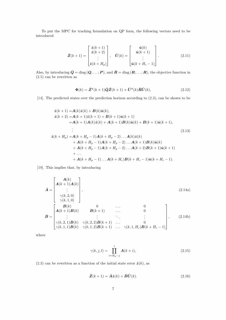
To put the MPC for tracking formulation on QP form, the following vectors need to beintroduced
Z(k + 1) =
z(k + 1)z(k + 2)
...z(k +Hp)
, U(k) =
u(k)u(k + 1)
...u(k +Hc − 1)
. (2.11)
Also, by introducing Q = diag (Q; . . . ;P ), and R = diag (R; . . . ;R), the objective function in(2.5) can be rewritten as
Φ(k) = Zᵀ(k + 1)QZ(k + 1) + Uᵀ(k)RU(k), (2.12)
[14]. The predicted states over the prediction horizon according to (2.3), can be shown to be
z(k + 1) =A(k)z(k) +B(k)u(k),
z(k + 2) =A(k + 1)z(k + 1) +B(k + 1)u(k + 1)
=A(k + 1)A(k)z(k) +A(k + 1)B(k)u(k) +B(k + 1)u(k + 1),
... (2.13)
z(k +Hp) =A(k +Hp − 1)A(k +Hp − 2) . . .A(k)z(k)
+A(k +Hp − 1)A(k +Hp − 2) . . .A(k + 1)B(k)u(k)
+A(k +Hp − 1)A(k +Hp − 2) . . .A(k + 2)B(k + 1)u(k + 1)
+ . . .
+A(k +Hp − 1) . . .A(k +Hc)B(k +Hc − 1)u(k +Hc − 1).
[19]. This implies that, by introducing
A =
A(k)A(k + 1)A(k)
...γ(k, 2, 0)γ(k, 1, 0)
, (2.14a)
B =
B(k) 0 . . . 0A(k + 1)B(k) B(k + 1) . . . 0
......
. . ....
γ(k, 2, 1)B(k) γ(k, 2, 2)B(k + 1) . . . 0γ(k, 1, 1)B(k) γ(k, 1, 2)B(k + 1) . . . γ(k, 1, Hc)B(k +Hc − 1)
, (2.14b)
where
γ(k, j, l) =
l∏
i=Hp−jA(k + i), (2.15)
(2.3) can be rewritten as a function of the initial state error z(k), as
Z(k + 1) = Az(k) + BU(k). (2.16)
7
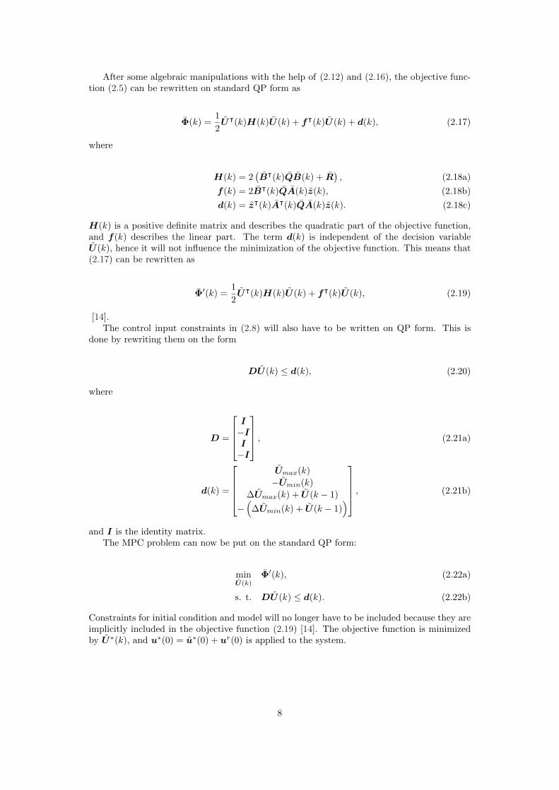
After some algebraic manipulations with the help of (2.12) and (2.16), the objective func-tion (2.5) can be rewritten on standard QP form as
Φ(k) =1
2Uᵀ(k)H(k)U(k) + fᵀ(k)U(k) + d(k), (2.17)
where
H(k) = 2(Bᵀ(k)QB(k) + R
), (2.18a)
f(k) = 2Bᵀ(k)QA(k)z(k), (2.18b)
d(k) = zᵀ(k)Aᵀ(k)QA(k)z(k). (2.18c)
H(k) is a positive definite matrix and describes the quadratic part of the objective function,and f(k) describes the linear part. The term d(k) is independent of the decision variableU(k), hence it will not influence the minimization of the objective function. This means that(2.17) can be rewritten as
Φ′(k) =1
2Uᵀ(k)H(k)U(k) + fᵀ(k)U(k), (2.19)
[14].The control input constraints in (2.8) will also have to be written on QP form. This is
done by rewriting them on the form
DU(k) ≤ d(k), (2.20)
where
D =
I−II−I
, (2.21a)
d(k) =
Umax(k)
−Umin(k)
∆Umax(k) + U(k − 1)
−(
∆Umin(k) + U(k − 1))
, (2.21b)
and I is the identity matrix.The MPC problem can now be put on the standard QP form:
minU(k)
Φ′(k), (2.22a)
s. t. DU(k) ≤ d(k). (2.22b)
Constraints for initial condition and model will no longer have to be included because they areimplicitly included in the objective function (2.19) [14]. The objective function is minimizedby U∗(k), and u∗(0) = u∗(0) + ur(0) is applied to the system.
8
Chapter 3
Vehicle Modeling
An MPC requires a model of the system, to use as the prediction model, which is used topredict the evolution of the system so that an optimal control input can be applied.
There are several different models to describe the dynamics of a car-like ground vehicle.There are two and four wheel models, kinematic and dynamic models, and the dynamics ofthe tires can be described by linear and nonlinear models [5, 6].
3.1 Bicycle Model
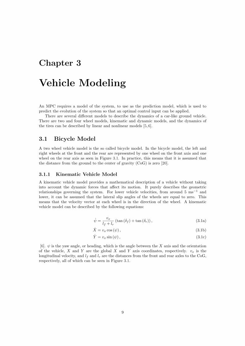
A two wheel vehicle model is the so called bicycle model. In the bicycle model, the left andright wheels at the front and the rear are represented by one wheel on the front axis and onewheel on the rear axis as seen in Figure 3.1. In practice, this means that it is assumed thatthe distance from the ground to the center of gravity (CoG) is zero [20].
3.1.1 Kinematic Vehicle Model
A kinematic vehicle model provides a mathematical description of a vehicle without takinginto account the dynamic forces that affect its motion. It purely describes the geometricrelationships governing the system. For lower vehicle velocities, from around 5 ms−1 andlower, it can be assumed that the lateral slip angles of the wheels are equal to zero. Thismeans that the velocity vector at each wheel is in the direction of the wheel. A kinematicvehicle model can be described by the following equations:
ψ =vx
lf + lr(tan (δf ) + tan (δr)) , (3.1a)
X = vx cos (ψ) , (3.1b)
Y = vx sin (ψ) , (3.1c)
[6]. ψ is the yaw angle, or heading, which is the angle between the X axis and the orientationof the vehicle, X and Y are the global X and Y axis coordinates, respectively. vx is thelongitudinal velocity, and lf and lr are the distances from the front and rear axles to the CoG,respectively, all of which can be seen in Figure 3.1.
9
X
Y
CoG
lr
lf
ψ
vx
δf
δr
Figure 3.1: Kinematic bicycle model of vehicle motion, which shows how vx, ψ, X, Y , δf , δr,lf , and lr are defined.
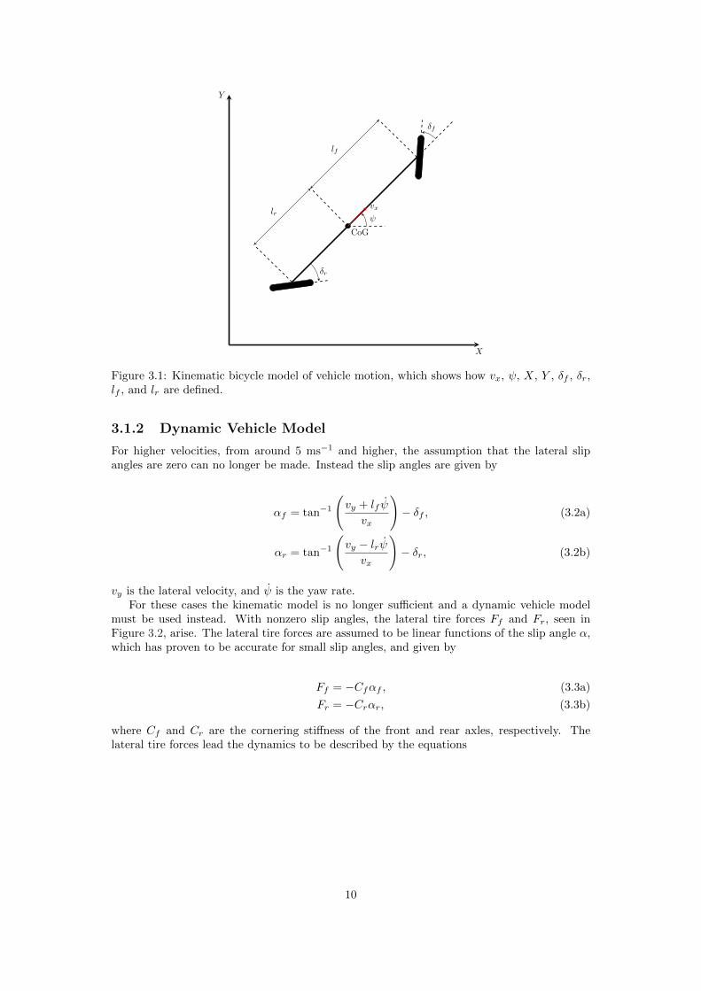
3.1.2 Dynamic Vehicle Model
For higher velocities, from around 5 ms−1 and higher, the assumption that the lateral slipangles are zero can no longer be made. Instead the slip angles are given by
αf = tan−1
(vy + lf ψ
vx
)− δf , (3.2a)
αr = tan−1
(vy − lrψ
vx
)− δr, (3.2b)
vy is the lateral velocity, and ψ is the yaw rate.For these cases the kinematic model is no longer sufficient and a dynamic vehicle model
must be used instead. With nonzero slip angles, the lateral tire forces Ff and Fr, seen inFigure 3.2, arise. The lateral tire forces are assumed to be linear functions of the slip angle α,which has proven to be accurate for small slip angles, and given by
Ff = −Cfαf , (3.3a)
Fr = −Crαr, (3.3b)
where Cf and Cr are the cornering stiffness of the front and rear axles, respectively. Thelateral tire forces lead the dynamics to be described by the equations
10
X
Y
CoG
lr
lf
ψ
ψ
vxvy
δf
αf
δrαr
Fr
Ff
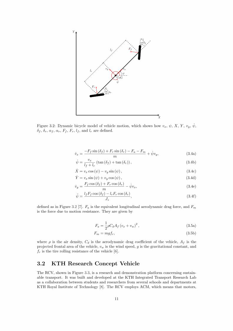
Figure 3.2: Dynamic bicycle model of vehicle motion, which shows how vx, ψ, X, Y , vy, ψ,δf , δr, αf , αr, Ff , Fr, lf , and lr are defined.
vx =−Ff sin (δf ) + Fr sin (δr)− Fa − Fm
m+ ψvy, (3.4a)
ψ =vx
lf + lr(tan (δf ) + tan (δr)) , (3.4b)
X = vx cos (ψ)− vy sin (ψ) , (3.4c)
Y = vx sin (ψ) + vy cos (ψ) , (3.4d)
vy =Ff cos (δf ) + Fr cos (δr)
m− ψvx, (3.4e)
ψ =lfFf cos (δf )− lrFr cos (δr)
Jz, (3.4f)
defined as in Figure 3.2 [7]. Fa is the equivalent longitudinal aerodynamic drag force, and Fmis the force due to motion resistance. They are given by
Fa =1
2ρCdAf (vx + vw)
2, (3.5a)
Fm = mgfr, (3.5b)
where ρ is the air density, Cd is the aerodynamic drag coefficient of the vehicle, Af is theprojected frontal area of the vehicle, vw is the wind speed, g is the gravitational constant, andfr is the tire rolling resistance of the vehicle [6].
3.2 KTH Research Concept Vehicle
The RCV, shown in Figure 3.3, is a research and demonstration platform concerning sustain-able transport. It was built and developed at the KTH Integrated Transport Research Labas a collaboration between students and researchers from several schools and departments atKTH Royal Institute of Technology [8]. The RCV employs ACM, which means that motors,
11
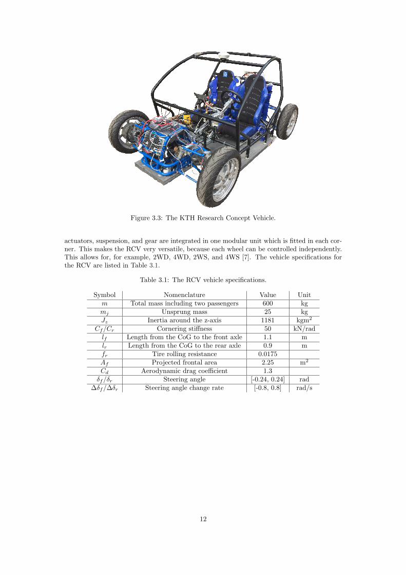
Figure 3.3: The KTH Research Concept Vehicle.
actuators, suspension, and gear are integrated in one modular unit which is fitted in each cor-ner. This makes the RCV very versatile, because each wheel can be controlled independently.This allows for, for example, 2WD, 4WD, 2WS, and 4WS [7]. The vehicle specifications forthe RCV are listed in Table 3.1.
Table 3.1: The RCV vehicle specifications.
Symbol Nomenclature Value Unitm Total mass including two passengers 600 kgmj Unsprung mass 25 kgJz Inertia around the z-axis 1181 kgm2
Cf/Cr Cornering stiffness 50 kN/radlf Length from the CoG to the front axle 1.1 mlr Length from the CoG to the rear axle 0.9 mfr Tire rolling resistance 0.0175Af Projected frontal area 2.25 m2
Cd Aerodynamic drag coefficient 1.3δf/δr Steering angle [-0.24, 0.24] rad
∆δf/∆δr Steering angle change rate [-0.8, 0.8] rad/s
12
Chapter 4
Path Following
One of the topics of research within autonomous driving, is path following. This means that apredetermined path, constituted by reference points, is generated offline or online. Each pointon the path includes the needed information, for example position, velocity, and heading, tomove the vehicle along the path in the desired way.
Different MPC designs are implemented to study how they perform when following differ-ent paths. The first MPC uses the kinematic vehicle model, as the prediction model, withlongitudinal acceleration ax and front wheel steering angle δf as the control inputs, which willbe referred to as the Kinematic 2WS MPC. The second one uses the dynamic vehicle modelin the MPC with ax and δf as the control inputs, the Dynamic 2WS MPC. The third oneuses the kinematic vehicle model with ax, δf , and rear wheel steering angle δr as the controlinputs, the Kinematic 4WS MPC. Finally, the fourth one uses the dynamic vehicle model withax, δf , and δr, as the control inputs, the Dynamic 4WS MPC.
The different designs are evaluated based on how small the deviation can be kept, whilekeeping the ride comfortable, on flat, sloped, and banked roads. The different tests andsimulation results are presented in Section 4.6.
The most suitable of the studied MPC designs is implemented for path following withthe RCV, to study how it performs in reality compared to in simulation, and the studies arepresented in Section 4.7.
4.1 Model Predictive Control
MPC is a good choice for path following, because of its ability to predict the evolution of thesystem to determine optimal control inputs, and the ease of implementing constraints.
4.1.1 Formulation
To use MPC for path following it needs to be formulated in the same way as the referencetracking MPC in Section 2.2, and the problem is also put on QP form as described in Section2.3. All simulations are run in Matlab, and the QP problem is solved using the tool CVXGEN[21].
4.1.2 Vehicle Models
In MPC a model of the system is used to predict the evolution over the prediction horizon. Twodifferent vehicle models are used as the MPC prediction model, and they are the discrete timerepresentation of the kinematic vehicle model in (3.1), and the discrete time representation ofthe dynamic bicycle model in (3.4), with the RCV specifications in Table 3.1.
Because ax is one of the control inputs, a state for the longitudinal velocity is added tothe kinematic model, and in the dynamic model, ax is added to the state describing the
13
[X0, Y0, ψ0] PathGenerator
[Xr,Y r]Controller
u∗Vehicle
z StateEstimator
z
Controller
[Xr,Y r] ReferenceGenerator
[Zr,U r]
z
U r
Zr
Linearize[A,B]
QP Form
[Φ′,D,d
]QP Solver U ∗ + u∗
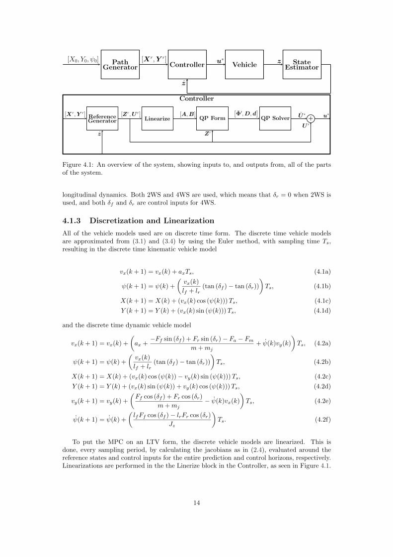
Figure 4.1: An overview of the system, showing inputs to, and outputs from, all of the partsof the system.
longitudinal dynamics. Both 2WS and 4WS are used, which means that δr = 0 when 2WS isused, and both δf and δr are control inputs for 4WS.
4.1.3 Discretization and Linearization
All of the vehicle models used are on discrete time form. The discrete time vehicle modelsare approximated from (3.1) and (3.4) by using the Euler method, with sampling time Ts,resulting in the discrete time kinematic vehicle model
vx(k + 1) = vx(k) + axTs, (4.1a)
ψ(k + 1) = ψ(k) +
(vx(k)
lf + lr(tan (δf )− tan (δr))
)Ts, (4.1b)
X(k + 1) = X(k) + (vx(k) cos (ψ(k)))Ts, (4.1c)
Y (k + 1) = Y (k) + (vx(k) sin (ψ(k)))Ts, (4.1d)
and the discrete time dynamic vehicle model
vx(k + 1) = vx(k) +
(ax +
−Ff sin (δf ) + Fr sin (δr)− Fa − Fmm+mj
+ ψ(k)vy(k)
)Ts, (4.2a)
ψ(k + 1) = ψ(k) +
(vx(k)
lf + lr(tan (δf )− tan (δr))
)Ts, (4.2b)
X(k + 1) = X(k) + (vx(k) cos (ψ(k))− vy(k) sin (ψ(k)))Ts, (4.2c)
Y (k + 1) = Y (k) + (vx(k) sin (ψ(k)) + vy(k) cos (ψ(k)))Ts, (4.2d)
vy(k + 1) = vy(k) +
(Ff cos (δf ) + Fr cos (δr)
m+mj− ψ(k)vx(k)
)Ts, (4.2e)
ψ(k + 1) = ψ(k) +
(lfFf cos (δf )− lrFr cos (δr)
Jz
)Ts. (4.2f)
To put the MPC on an LTV form, the discrete vehicle models are linearized. This isdone, every sampling period, by calculating the jacobians as in (2.4), evaluated around thereference states and control inputs for the entire prediction and control horizons, respectively.Linearizations are performed in the the Linerize block in the Controller, as seen in Figure 4.1.
14
−0.5 0 0.5 1 1.5 2 2.5 3 3.5 4 4.5
0
0.5
1
1.5
2
2.5
3
3.5
4
[Xr(n),Y r(n)]
[X0, Y0]
X [m]
Y[m
]
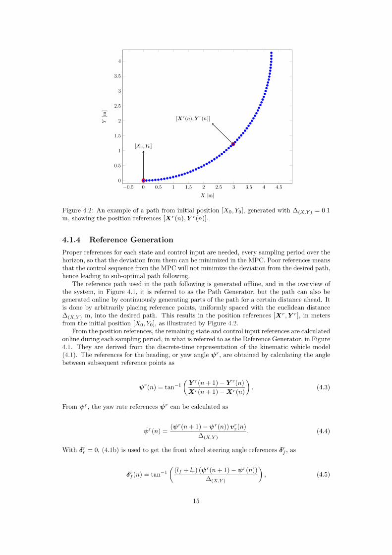
Figure 4.2: An example of a path from initial position [X0, Y0], generated with ∆(X,Y ) = 0.1m, showing the position references [Xr(n),Y r(n)].
4.1.4 Reference Generation
Proper references for each state and control input are needed, every sampling period over thehorizon, so that the deviation from them can be minimized in the MPC. Poor references meansthat the control sequence from the MPC will not minimize the deviation from the desired path,hence leading to sub-optimal path following.
The reference path used in the path following is generated offline, and in the overview ofthe system, in Figure 4.1, it is referred to as the Path Generator, but the path can also begenerated online by continuously generating parts of the path for a certain distance ahead. Itis done by arbitrarily placing reference points, uniformly spaced with the euclidean distance∆(X,Y ) m, into the desired path. This results in the position references [Xr,Y r], in metersfrom the initial position [X0, Y0], as illustrated by Figure 4.2.
From the position references, the remaining state and control input references are calculatedonline during each sampling period, in what is referred to as the Reference Generator, in Figure4.1. They are derived from the discrete-time representation of the kinematic vehicle model(4.1). The references for the heading, or yaw angle ψr, are obtained by calculating the anglebetween subsequent reference points as
ψr(n) = tan−1(Y r(n+ 1)− Y r(n)
Xr(n+ 1)−Xr(n)
). (4.3)
From ψr, the yaw rate references ψr can be calculated as
ψr(n) =(ψr(n+ 1)−ψr(n))vrx(n)
∆(X,Y ). (4.4)
With δrr = 0, (4.1b) is used to get the front wheel steering angle references δrf , as
δrf (n) = tan−1(
(lf + lr) (ψr(n+ 1)−ψr(n))
∆(X,Y )
), (4.5)
15
and similarly, δrr = −δrf , leads δrf to be
δrf (n) = tan−1(
(lf + lr) (ψr(n+ 1)−ψr(n))
2∆(X,Y )
). (4.6)
The references for the lateral velocity vry(n) = 0, because keeping the lateral velocity downmeans that the deviation from the path is easier to keep down and the ride is more comfortable.For the purpose of comparing the different MPC design strategies, the longitudinal velocityreferences vrx(n) are kept constant for the entire paths, and the longitudinal accelerationreferences arx(n) = 0.
By using the equations in (4.3) - (4.6), it is possible to acquire references for all of thestates and control inputs for each of the reference points. To find the appropriate references,at each sampling instant, the reference point on the path with the shortest euclidean distanceto the current position is found. When the closest reference point on the path is known,Hp reference points ahead are used for calculating the state and control input references forthe entire prediction horizon. When finding the Hp reference points, not every consecutivereference point is used. Based on the current velocity vx(k), the distance between the referencepoints ∆(X,Y ), and the sampling time Ts, the reference points to use are determined by
ζ =
⌈vx(k)Ts∆(X,Y )
⌉. (4.7)
With [Xr(n),Y r(n)] as the closest reference point to the current position, the reference points[Xr(n+ ξ),Y r(n+ ξ)], where ξ ∈ [0, ζHp − ζ], are used to calculate references for the statesand control inputs with (4.3) - (4.6). This results in Zr = {zr(n), zr(n+ ζ), . . . ,zr(n+ ζHp−ζ)}, and U r = {ur(n),ur(n+ζ), . . . ,ur(n+ζHp−ζ)}, which are outputted from the ReferenceGenerator block, as shown in Figure 4.1.
4.1.5 State Estimation
The MPC relies on getting the current state of the vehicle at each sampling instant, becauseit is used as the initial condition for the optimization problem. At the beginning of eachsampling period the current state is sent to the controller. In simulations the current statescan be sent flawlessly from the simulation model to the controller. However, this is not thecase in reality, where the states have to be measured with different kinds of sensors. Thesensors include, for example, GPS, which can give the velocity, heading, and position of thevehicle. The sensor data from a GPS can be combined with the sensor data from, for example,an inertial measurement unit (IMU) to get more accurate estimations of the current state ofthe vehicle. State estimations are performed in the State Estimator block, in Figure 4.1, whichsends the estimated current states z(k) to the controller.
4.2 Ride Comfort
Ride comfort is hard to quantify, because it is subjective what is comfortable and what is not.When designing highways, two key aspects of keeping the ride comfort, is to design them sothat the lateral acceleration and lateral jerk are kept below certain values. According to [22],for the lateral acceleration it varies between 1.47 − 2.45 ms−2. For the lateral jerk, which isthe time derivative of the lateral acceleration, it is between 0.3− 0.9 ms−3.
Similarly, longitudinal acceleration and longitudinal jerk also impact the ride comfort. Withthe longitudinal acceleration ax as one of the control inputs, staying within the comfortablelimits for longitudinal acceleration and jerk is easy. This is because of the ease of directlyconstraining ax and the rate at which it can change per second, ∆ax, in the MPC.
Staying within the limits for lateral acceleration ay and jerk ∆ay is more difficult, becausethey cannot be controlled directly. Instead they can be indirectly controlled by the entering
16
speed into corners and by constraining the rate at which the front and rear wheel steeringangles are allowed to change, ∆δf and ∆δr, respectively.
4.3 Banked Road
The banking of the road can be modeled as a force acting on the vehicle, which affects thelateral dynamics. This is done by modifying (4.2e) to
vy(k + 1) = vy(k) +
(Ff cos (δf ) + Fr cos (δr) + Fb
m+mj− ψ(k)vx(k)
)Ts, (4.8)
where the force due to banking is
Fb = (m+mj)g sin(φ), (4.9)
g is the gravitational constant, and φ is the banking angle [6].
4.4 Sloping Road
The slope of the road can be modeled as a force acting on the vehicle, which affects thelongitudinal dynamics. This is done by modifying (4.2a) to
vx(k + 1) = vx(k) +
(ax +
−Ff sin (δf ) + Fr sin (δr)− Fa − Fm − Fsm+mj
+ ψ(k)vy(k)
)Ts,
(4.10)
where the force due to sloping is
Fs = (m+mj)g sin(θ), (4.11)
g is the gravitational constant, and θ is the sloping angle [6].
4.5 Sampling Time
The choice of sampling time influences the horizon, which is the distance on the path which isused to predict the behavior of the vehicle. A longer sampling period means that the horizon isincreased, but leads to that the discretized prediction model is less accurate. Having a longersampling period also means that it may be possible to increase the prediction and controlhorizons to further increase the horizon on the path. This means that a shorter samplingperiod leads to a shorter horizon, which may be further reduced because it may be necessaryto decrease the prediction and control horizons. The benefit of a shorter sampling period isthe improved accuracy of the prediction model.
The shortest feasible sampling time, for the implementation with the RCV, is 0.05 s, seeSection 4.7.2. The sampling time 0.01 s discarded, because it leads to a horizon that is tooshort and it is far from a feasible sampling time for the implementation with the RCV. Inorder to have a more feasible sampling time and a longer horizon, while keeping the predictionaccuracy at an acceptable level, 0.03 s is chosen as the sampling time for the simulation studies.
17
4.6 Path Following Simulation Results
Two path following simulation tests are performed to evaluate the performance of the variousMPC designs, including the Kinematic 2WS MPC, the Dynamic 2WS MPC, the Kinematic4WS MPC, and the Dynamic 4WS MPC. The tests include tests on a flat, sloped and bankedroads, with and without disturbances.
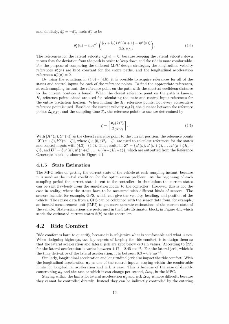
One test is a u-turn test on a flat road. The purpose of the u-turn test on a flat road,referred to as the u-turn test, is done to the evaluate the performance by testing how sharplya u-turn with constant curvature can be made without causing the position deviation ε to belarger than 0.3 m and keeping the lateral acceleration ay below 1.47 ms−2, which is consideredthe maximum to maintain the ride comfort. The deviation ε is the euclidean distance to thereference point closest to the current position. A u-turn with a constant curvature results in astep in the steering angle reference, and the radius for the different paths is determined by apercentage of the maximum front wheel steering angle, for example 45% of the maximum frontwheel steering angle results in the path in Figure 4.3, which has 18.45 m radius u-turn. Testsare run at 13.89 ms−1 (50 kph), without disturbances, and the steering angle change rates∆δf and ∆δr are constrained to make the ride as comfortable as possible without causing thevehicle to deviate more than allowed.
0 10 20 30 40 50 60 70 80 90 100 1100
10
20
30
X [m]
Y[m
]
Figure 4.3: A path with a u-turn equivalent to 45% of a full turn with 18.45 m radius.
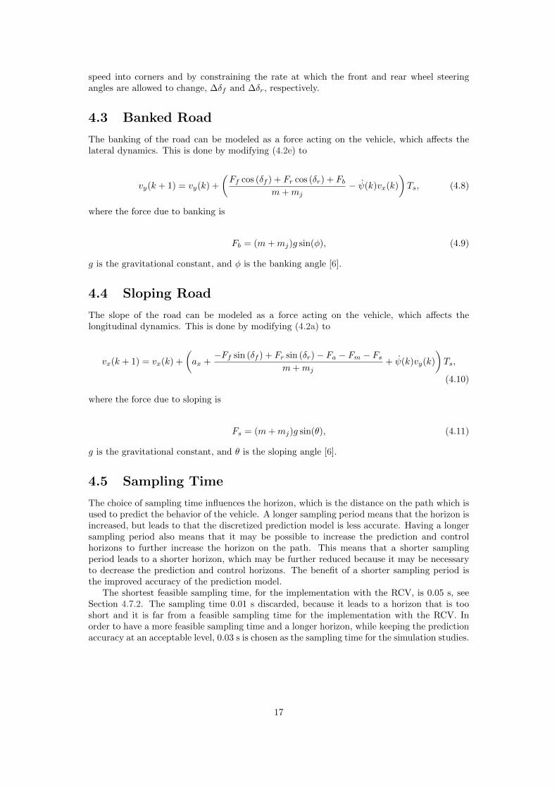
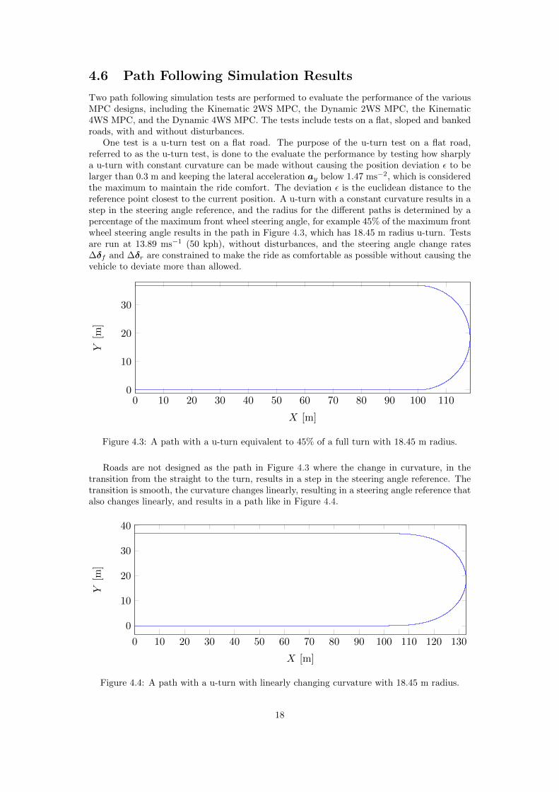
Roads are not designed as the path in Figure 4.3 where the change in curvature, in thetransition from the straight to the turn, results in a step in the steering angle reference. Thetransition is smooth, the curvature changes linearly, resulting in a steering angle reference thatalso changes linearly, and results in a path like in Figure 4.4.
0 10 20 30 40 50 60 70 80 90 100 110 120 130
0
10
20
30
40
X [m]
Y[m
]
Figure 4.4: A path with a u-turn with linearly changing curvature with 18.45 m radius.
18
Other tests are s-turn tests, which are performed on path with linearly changing curvature,referred to as the s-turn tests, with the purpose to test how the MPC implementations handlemeasurement disturbances. This is done by adding simulated disturbances to the each of thestates that are sent to the MPC, corresponding the the accuracy of the sensors used in theexperimental test, see Section 4.7.1. The standard deviation σ of the added disturbances areshown in Table 4.1.
Table 4.1: The accuracy of the sensors used.
vx[ms−1
]ψ [rad] X [m] Y [m] vy
[ms−1
]ψ [rad/s]
σ 0.1 0.018 0.015 0.015 0.1 0.018
To the position, X and Y , there is also added measurement uncertainty of the network RTKof ± 0.025 m.
A test in which a u-turn is performed on a downhill slope is also conducted. The purposewith the u-turn test on a downhill slope is done to study the performance when the road is nolonger flat. The performance is evaluated based on how low the deviation can be kept whilekeeping the lateral acceleration below 1.47 ms−2. Entering at 13.89 ms−1 (50 kph), a u-turnis performed on a 10% downhill slope.
The paths used in the simulations are generated with ∆(X,Y ) = 0.01 m, the sampling timeused is Ts = 0.03 s, and the prediction and control horizons are, Hp = 24 and Hc = 19,respectively. All simulations are run with the discrete time kinematic vehicle model, in (4.1),for velocities below 5 ms−1, and the discrete time dynamic vehicle model, in (4.2), modifiedto include the forces due to road banking and slope as shown in Section 4.3 and Section4.4, for velocities above 5 ms−1, as the simulation models. The simulation models have thespecifications of the RCV, in Table 3.1, and the wind speed vw = 0. The constraints that areused on the steering angles δf and δr are due to physical limitations of the RCV, presentedin Section 4.1.2, which means that means that −0.24 ≤ δf , δr ≤ 0.24 rad. Constraints on thesteering angles change rates ∆δf and ∆δr are determined to make the ride comfort, describedin Section 4.2, as good as possible, which is different from case to case. The constraints on thelongitudinal acceleration ax are due to ride comfort, presented in Section 4.2, which meansthat −2.45 ≤ ax ≤ 2.45 ms−2, and −0.9 ≤ ∆ax ≤ 0.9 ms−3.
4.6.1 Kinematic 2WS MPC and Dynamic 2WS MPC
To study the performance of the Kinematic 2WS MPC compared to the Dynamic 2WS MPCseveral tests are conducted. They include tests on flat, sloped, and banked roads, with andwithout disturbances.
U-Turn on a Flat Road
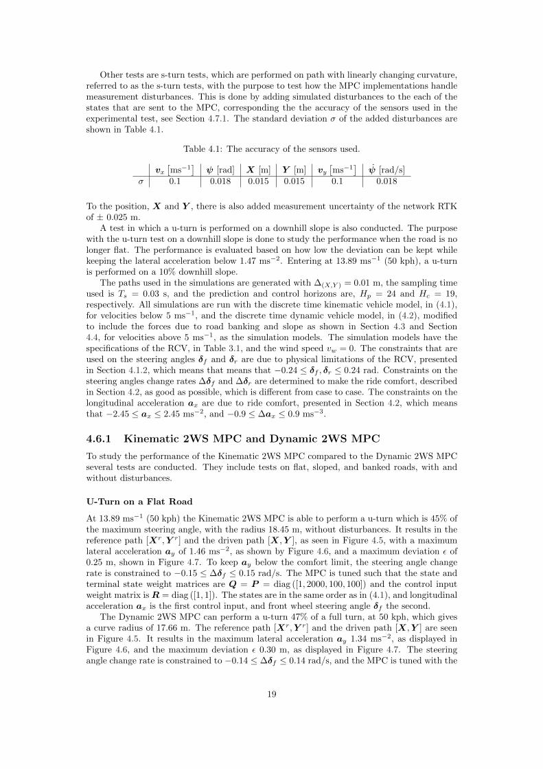
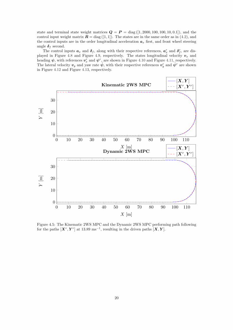
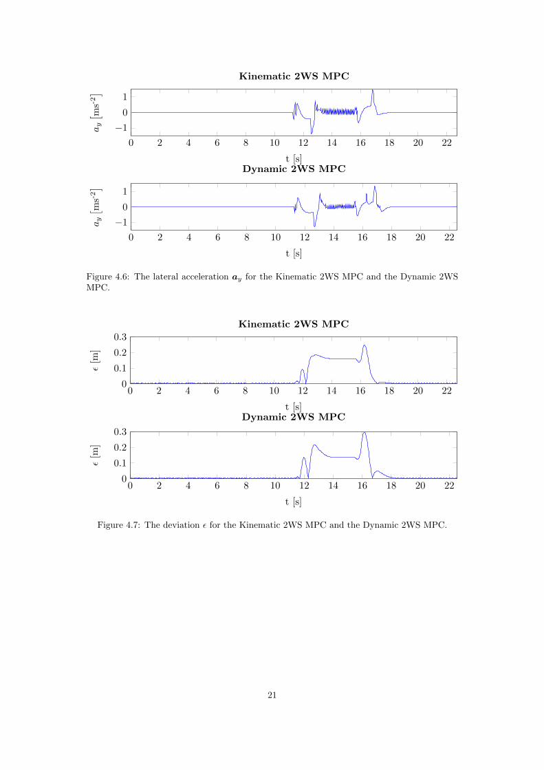
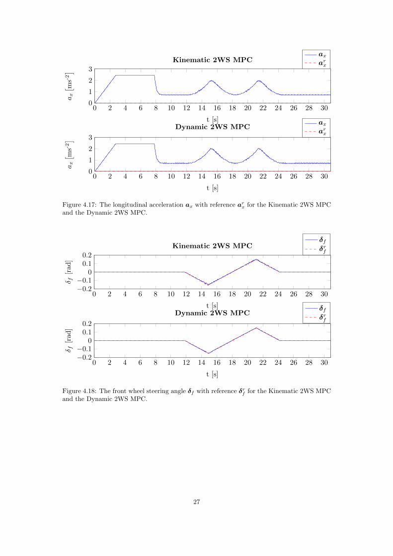
At 13.89 ms−1 (50 kph) the Kinematic 2WS MPC is able to perform a u-turn which is 45% ofthe maximum steering angle, with the radius 18.45 m, without disturbances. It results in thereference path [Xr,Y r] and the driven path [X,Y ], as seen in Figure 4.5, with a maximumlateral acceleration ay of 1.46 ms−2, as shown by Figure 4.6, and a maximum deviation ε of0.25 m, shown in Figure 4.7. To keep ay below the comfort limit, the steering angle changerate is constrained to −0.15 ≤ ∆δf ≤ 0.15 rad/s. The MPC is tuned such that the state andterminal state weight matrices are Q = P = diag ([1, 2000, 100, 100]) and the control inputweight matrix isR = diag ([1, 1]). The states are in the same order as in (4.1), and longitudinalacceleration ax is the first control input, and front wheel steering angle δf the second.
The Dynamic 2WS MPC can perform a u-turn 47% of a full turn, at 50 kph, which givesa curve radius of 17.66 m. The reference path [Xr,Y r] and the driven path [X,Y ] are seenin Figure 4.5. It results in the maximum lateral acceleration ay 1.34 ms−2, as displayed inFigure 4.6, and the maximum deviation ε 0.30 m, as displayed in Figure 4.7. The steeringangle change rate is constrained to −0.14 ≤ ∆δf ≤ 0.14 rad/s, and the MPC is tuned with the
19
state and terminal state weight matrices Q = P = diag ([1, 2000, 100, 100, 10, 0.1]), and thecontrol input weight matrix R = diag ([1, 1]). The states are in the same order as in (4.2), andthe control inputs are in the order longitudinal acceleration ax first, and front wheel steeringangle δf second.
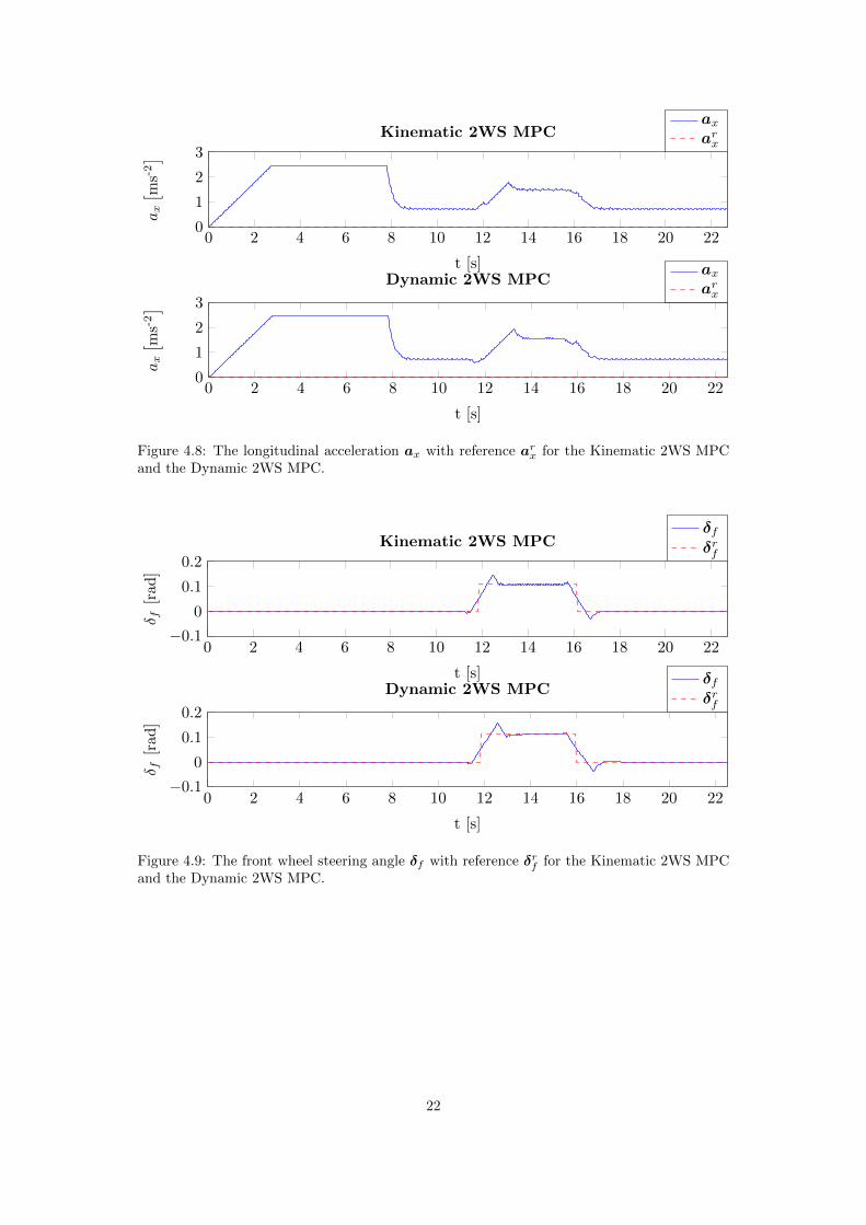
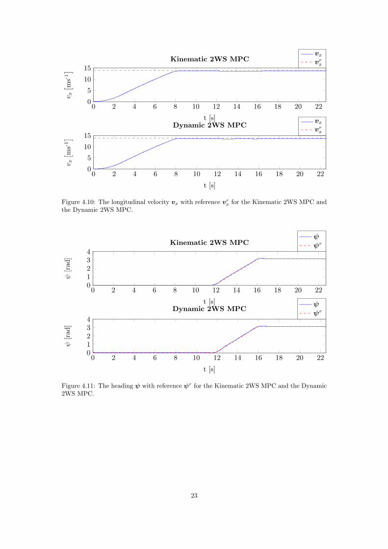
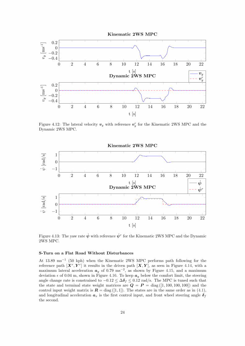
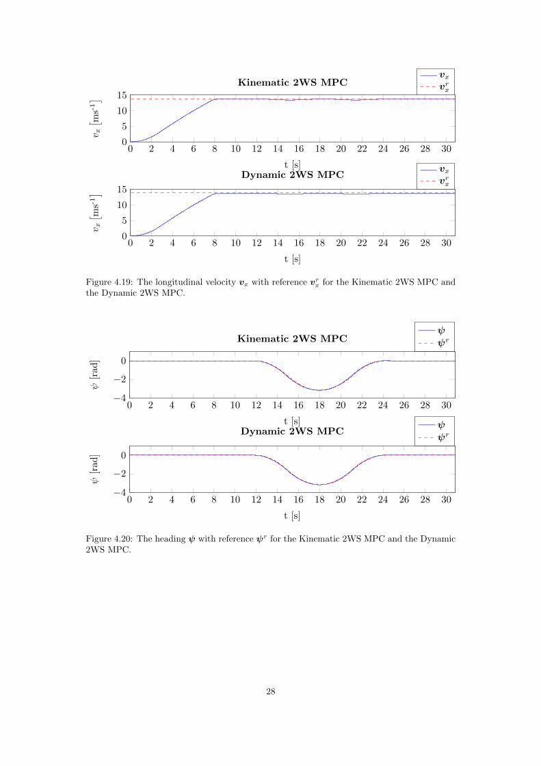
The control inputs ax and δf , along with their respective references, arx and δrf , are dis-played in Figure 4.8 and Figure 4.9, respectively. The states longitudinal velocity vx andheading ψ, with references vrx and ψr, are shown in Figure 4.10 and Figure 4.11, respectively.The lateral velocity vy and yaw rate ψ, with their respective references vry and ψr are shownin Figure 4.12 and Figure 4.13, respectively.
0 10 20 30 40 50 60 70 80 90 100 1100
10
20
30
X [m]
Y[m
]
Kinematic 2WS MPC[X,Y ]
[Xr,Y r]
0 10 20 30 40 50 60 70 80 90 100 1100
10
20
30
X [m]
Y[m
]
Dynamic 2WS MPC[X,Y ]
[Xr,Y r]
Figure 4.5: The Kinematic 2WS MPC and the Dynamic 2WS MPC performing path followingfor the paths [Xr,Y r] at 13.89 ms−1, resulting in the driven paths [X,Y ].
20
0 2 4 6 8 10 12 14 16 18 20 22
−1
0
1
t [s]
ay
[ ms-2]
Kinematic 2WS MPC
0 2 4 6 8 10 12 14 16 18 20 22
−1
0
1
t [s]
ay
[ ms-2]
Dynamic 2WS MPC
Figure 4.6: The lateral acceleration ay for the Kinematic 2WS MPC and the Dynamic 2WSMPC.
0 2 4 6 8 10 12 14 16 18 20 220
0.1
0.2
0.3
t [s]
ε[m
]
Kinematic 2WS MPC
0 2 4 6 8 10 12 14 16 18 20 220
0.1
0.2
0.3
t [s]
ε[m
]
Dynamic 2WS MPC
Figure 4.7: The deviation ε for the Kinematic 2WS MPC and the Dynamic 2WS MPC.
21
0 2 4 6 8 10 12 14 16 18 20 220
1
2
3
t [s]
ax
[ ms-2]
Kinematic 2WS MPCax
arx
0 2 4 6 8 10 12 14 16 18 20 220
1
2
3
t [s]
ax
[ ms-2]
Dynamic 2WS MPCax
arx
Figure 4.8: The longitudinal acceleration ax with reference arx for the Kinematic 2WS MPCand the Dynamic 2WS MPC.
0 2 4 6 8 10 12 14 16 18 20 22−0.1
0
0.1
0.2
t [s]
δ f[rad
]
Kinematic 2WS MPCδfδrf
0 2 4 6 8 10 12 14 16 18 20 22−0.1
0
0.1
0.2
t [s]
δ f[rad
]
Dynamic 2WS MPCδfδrf
Figure 4.9: The front wheel steering angle δf with reference δrf for the Kinematic 2WS MPCand the Dynamic 2WS MPC.
22
0 2 4 6 8 10 12 14 16 18 20 220
5
10
15
t [s]
v x[ m
s-1]
Kinematic 2WS MPCvxvrx
0 2 4 6 8 10 12 14 16 18 20 220
5
10
15
t [s]
v x[ m
s-1]
Dynamic 2WS MPCvxvrx
Figure 4.10: The longitudinal velocity vx with reference vrx for the Kinematic 2WS MPC andthe Dynamic 2WS MPC.
0 2 4 6 8 10 12 14 16 18 20 2201234
t [s]
ψ[rad
]
Kinematic 2WS MPCψψr
0 2 4 6 8 10 12 14 16 18 20 2201234
t [s]
ψ[rad
]
Dynamic 2WS MPCψψr
Figure 4.11: The heading ψ with reference ψr for the Kinematic 2WS MPC and the Dynamic2WS MPC.
23
0 2 4 6 8 10 12 14 16 18 20 22
−0.4−0.2
00.2
t [s]
v y[ m
s-1]
Kinematic 2WS MPC
0 2 4 6 8 10 12 14 16 18 20 22
−0.4−0.2
00.2
t [s]
v y[ m
s-1]
Dynamic 2WS MPCvyvry
Figure 4.12: The lateral velocity vy with reference vry for the Kinematic 2WS MPC and theDynamic 2WS MPC.
0 2 4 6 8 10 12 14 16 18 20 22
−1
0
1
t [s]
ψ[rad
/s]
Kinematic 2WS MPC
0 2 4 6 8 10 12 14 16 18 20 22
−1
0
1
t [s]
ψ[rad
/s]
Dynamic 2WS MPCψ
ψr
Figure 4.13: The yaw rate ψ with reference ψr for the Kinematic 2WS MPC and the Dynamic2WS MPC.
S-Turn on a Flat Road Without Disturbances
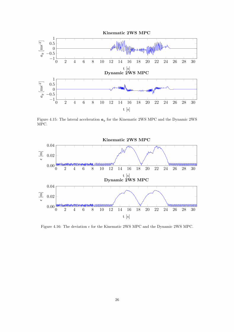
At 13.89 ms−1 (50 kph) when the Kinematic 2WS MPC performs path following for thereference path [Xr,Y r] it results in the driven path [X,Y ], as seen in Figure 4.14, with amaximum lateral acceleration ay of 0.79 ms−2, as shown by Figure 4.15, and a maximumdeviation ε of 0.04 m, shown in Figure 4.16. To keep ay below the comfort limit, the steeringangle change rate is constrained to −0.12 ≤ ∆δf ≤ 0.12 rad/s. The MPC is tuned such thatthe state and terminal state weight matrices are Q = P = diag ([1, 100, 100, 100]) and thecontrol input weight matrix is R = diag ([1, 1]). The states are in the same order as in (4.1),and longitudinal acceleration ax is the first control input, and front wheel steering angle δfthe second.
24
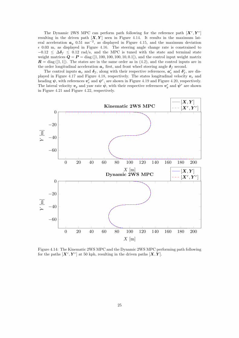
The Dynamic 2WS MPC can perform path following for the reference path [Xr,Y r]resulting in the driven path [X,Y ] seen in Figure 4.14. It results in the maximum lat-eral acceleration ay 0.51 ms−2, as displayed in Figure 4.15, and the maximum deviationε 0.03 m, as displayed in Figure 4.16. The steering angle change rate is constrained to−0.12 ≤ ∆δf ≤ 0.12 rad/s, and the MPC is tuned with the state and terminal stateweight matrices Q = P = diag ([1, 100, 100, 100, 10, 0.1]), and the control input weight matrixR = diag ([1, 1]). The states are in the same order as in (4.2), and the control inputs are inthe order longitudinal acceleration ax first, and front wheel steering angle δf second.
The control inputs ax and δf , along with their respective references, arx and δrf , are dis-played in Figure 4.17 and Figure 4.18, respectively. The states longitudinal velocity vx andheading ψ, with references vrx and ψr, are shown in Figure 4.19 and Figure 4.20, respectively.The lateral velocity vy and yaw rate ψ, with their respective references vry and ψr are shownin Figure 4.21 and Figure 4.22, respectively.
0 20 40 60 80 100 120 140 160 180 200
−60
−40
−20
0
X [m]
Y[m
]
Kinematic 2WS MPC[X,Y ]
[Xr,Y r]
0 20 40 60 80 100 120 140 160 180 200
−60
−40
−20
0
X [m]
Y[m
]
Dynamic 2WS MPC[X,Y ]
[Xr,Y r]
Figure 4.14: The Kinematic 2WS MPC and the Dynamic 2WS MPC performing path followingfor the paths [Xr,Y r] at 50 kph, resulting in the driven paths [X,Y ].
25
0 2 4 6 8 10 12 14 16 18 20 22 24 26 28 30−1
−0.50
0.51
t [s]
ay
[ ms-2]
Kinematic 2WS MPC
0 2 4 6 8 10 12 14 16 18 20 22 24 26 28 30−1
−0.50
0.51
t [s]
ay
[ ms-2]
Dynamic 2WS MPC
Figure 4.15: The lateral acceleration ay for the Kinematic 2WS MPC and the Dynamic 2WSMPC.
0 2 4 6 8 10 12 14 16 18 20 22 24 26 28 300.00
0.02
0.04
t [s]
ε[m
]
Kinematic 2WS MPC
0 2 4 6 8 10 12 14 16 18 20 22 24 26 28 300.00
0.02
0.04
t [s]
ε[m
]
Dynamic 2WS MPC
Figure 4.16: The deviation ε for the Kinematic 2WS MPC and the Dynamic 2WS MPC.
26
0 2 4 6 8 10 12 14 16 18 20 22 24 26 28 300
1
2
3
t [s]
ax
[ ms-2]
Kinematic 2WS MPCax
arx
0 2 4 6 8 10 12 14 16 18 20 22 24 26 28 300
1
2
3
t [s]
ax
[ ms-2]
Dynamic 2WS MPCax
arx
Figure 4.17: The longitudinal acceleration ax with reference arx for the Kinematic 2WS MPCand the Dynamic 2WS MPC.
0 2 4 6 8 10 12 14 16 18 20 22 24 26 28 30−0.2−0.1
00.10.2
t [s]
δ f[rad
]
Kinematic 2WS MPCδfδrf
0 2 4 6 8 10 12 14 16 18 20 22 24 26 28 30−0.2−0.1
00.10.2
t [s]
δ f[rad
]
Dynamic 2WS MPCδfδrf
Figure 4.18: The front wheel steering angle δf with reference δrf for the Kinematic 2WS MPCand the Dynamic 2WS MPC.
27
0 2 4 6 8 10 12 14 16 18 20 22 24 26 28 300
5
10
15
t [s]
v x[ m
s-1]
Kinematic 2WS MPCvxvrx
0 2 4 6 8 10 12 14 16 18 20 22 24 26 28 300
5
10
15
t [s]
v x[ m
s-1]
Dynamic 2WS MPCvxvrx
Figure 4.19: The longitudinal velocity vx with reference vrx for the Kinematic 2WS MPC andthe Dynamic 2WS MPC.
0 2 4 6 8 10 12 14 16 18 20 22 24 26 28 30−4
−2
0
t [s]
ψ[rad]
Kinematic 2WS MPCψψr
0 2 4 6 8 10 12 14 16 18 20 22 24 26 28 30−4
−2
0
t [s]
ψ[rad]
Dynamic 2WS MPCψψr
Figure 4.20: The heading ψ with reference ψr for the Kinematic 2WS MPC and the Dynamic2WS MPC.
28
0 2 4 6 8 10 12 14 16 18 20 22 24 26 28 30−0.4−0.2
00.20.4
t [s]
v y[ m
s-1]
Kinematic 2WS MPC
0 2 4 6 8 10 12 14 16 18 20 22 24 26 28 30−0.4−0.2
00.20.4
t [s]
v y[ m
s-1]
Dynamic 2WS MPCvyvry
Figure 4.21: The lateral velocity vy with reference vry for the Kinematic 2WS MPC and theDynamic 2WS MPC.
0 2 4 6 8 10 12 14 16 18 20 22 24 26 28 30−2−1012
t [s]
ψ[rad
/s]
Kinematic 2WS MPC
0 2 4 6 8 10 12 14 16 18 20 22 24 26 28 30−2−1012
t [s]
ψ[rad
/s]
Dynamic 2WS MPCψ
ψr
Figure 4.22: The yaw rate ψ with reference ψr for the Kinematic 2WS MPC and the Dynamic2WS MPC.
S-Turn on a Flat Road With Disturbances
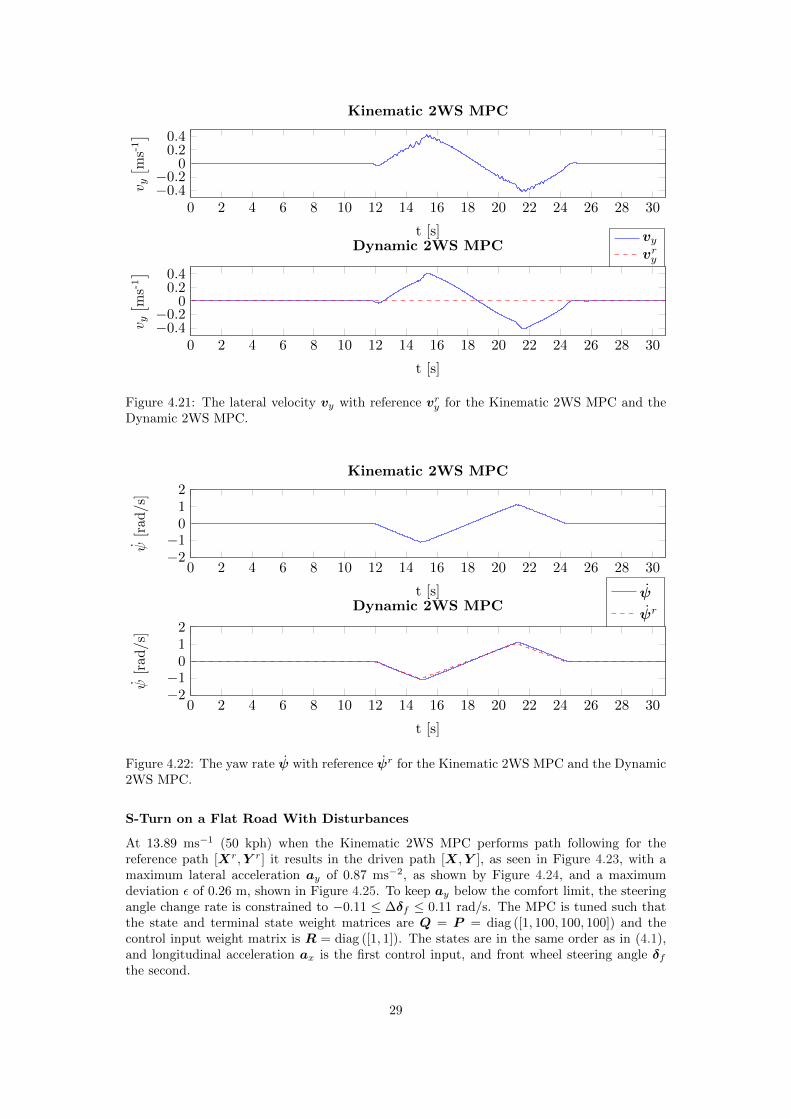
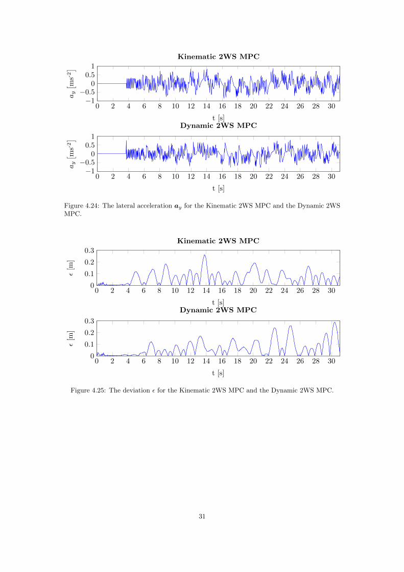
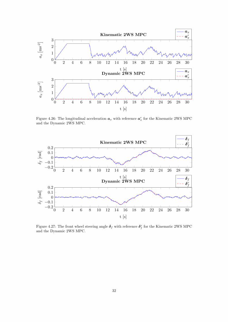
At 13.89 ms−1 (50 kph) when the Kinematic 2WS MPC performs path following for thereference path [Xr,Y r] it results in the driven path [X,Y ], as seen in Figure 4.23, with amaximum lateral acceleration ay of 0.87 ms−2, as shown by Figure 4.24, and a maximumdeviation ε of 0.26 m, shown in Figure 4.25. To keep ay below the comfort limit, the steeringangle change rate is constrained to −0.11 ≤ ∆δf ≤ 0.11 rad/s. The MPC is tuned such thatthe state and terminal state weight matrices are Q = P = diag ([1, 100, 100, 100]) and thecontrol input weight matrix is R = diag ([1, 1]). The states are in the same order as in (4.1),and longitudinal acceleration ax is the first control input, and front wheel steering angle δfthe second.
29
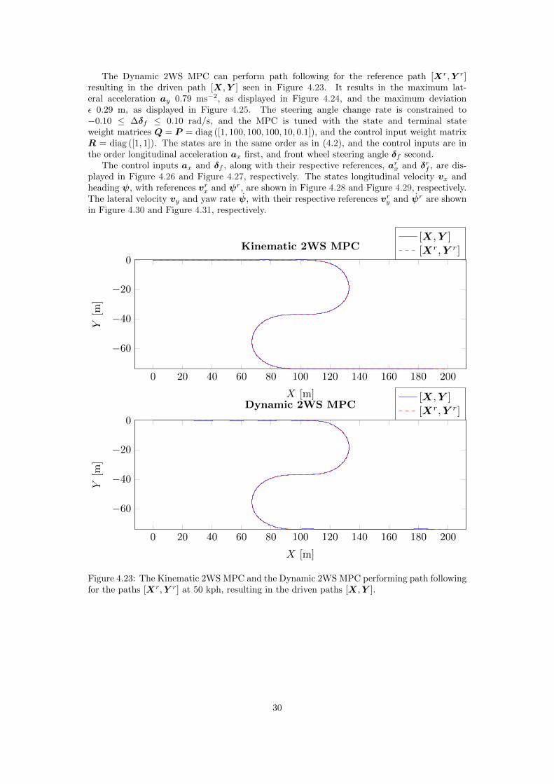
The Dynamic 2WS MPC can perform path following for the reference path [Xr,Y r]resulting in the driven path [X,Y ] seen in Figure 4.23. It results in the maximum lat-eral acceleration ay 0.79 ms−2, as displayed in Figure 4.24, and the maximum deviationε 0.29 m, as displayed in Figure 4.25. The steering angle change rate is constrained to−0.10 ≤ ∆δf ≤ 0.10 rad/s, and the MPC is tuned with the state and terminal stateweight matrices Q = P = diag ([1, 100, 100, 100, 10, 0.1]), and the control input weight matrixR = diag ([1, 1]). The states are in the same order as in (4.2), and the control inputs are inthe order longitudinal acceleration ax first, and front wheel steering angle δf second.
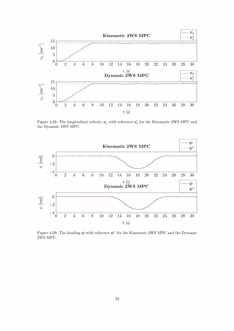
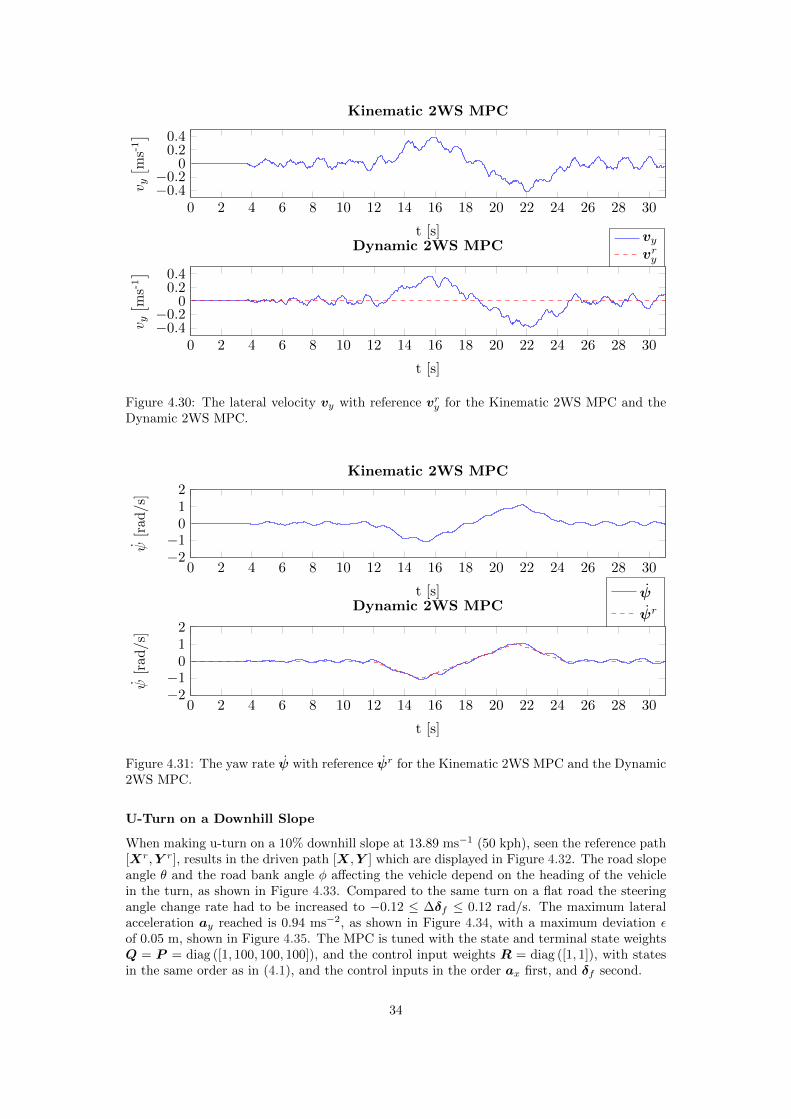
The control inputs ax and δf , along with their respective references, arx and δrf , are dis-played in Figure 4.26 and Figure 4.27, respectively. The states longitudinal velocity vx andheading ψ, with references vrx and ψr, are shown in Figure 4.28 and Figure 4.29, respectively.The lateral velocity vy and yaw rate ψ, with their respective references vry and ψr are shownin Figure 4.30 and Figure 4.31, respectively.
0 20 40 60 80 100 120 140 160 180 200
−60
−40
−20
0
X [m]
Y[m
]
Kinematic 2WS MPC[X,Y ]
[Xr,Y r]
0 20 40 60 80 100 120 140 160 180 200
−60
−40
−20
0
X [m]
Y[m
]
Dynamic 2WS MPC[X,Y ]
[Xr,Y r]
Figure 4.23: The Kinematic 2WS MPC and the Dynamic 2WS MPC performing path followingfor the paths [Xr,Y r] at 50 kph, resulting in the driven paths [X,Y ].
30
0 2 4 6 8 10 12 14 16 18 20 22 24 26 28 30−1
−0.50
0.51
t [s]
ay
[ ms-2]
Kinematic 2WS MPC
0 2 4 6 8 10 12 14 16 18 20 22 24 26 28 30−1
−0.50
0.51
t [s]
ay
[ ms-2]
Dynamic 2WS MPC
Figure 4.24: The lateral acceleration ay for the Kinematic 2WS MPC and the Dynamic 2WSMPC.
0 2 4 6 8 10 12 14 16 18 20 22 24 26 28 300
0.1
0.2
0.3
t [s]
ε[m
]
Kinematic 2WS MPC
0 2 4 6 8 10 12 14 16 18 20 22 24 26 28 300
0.1
0.2
0.3
t [s]
ε[m
]
Dynamic 2WS MPC
Figure 4.25: The deviation ε for the Kinematic 2WS MPC and the Dynamic 2WS MPC.
31
0 2 4 6 8 10 12 14 16 18 20 22 24 26 28 300
1
2
3
t [s]
ax
[ ms-2]
Kinematic 2WS MPCax
arx
0 2 4 6 8 10 12 14 16 18 20 22 24 26 28 300
1
2
3
t [s]
ax
[ ms-2]
Dynamic 2WS MPCax
arx
Figure 4.26: The longitudinal acceleration ax with reference arx for the Kinematic 2WS MPCand the Dynamic 2WS MPC.
0 2 4 6 8 10 12 14 16 18 20 22 24 26 28 30−0.2−0.1
00.10.2
t [s]
δ f[rad
]
Kinematic 2WS MPCδfδrf
0 2 4 6 8 10 12 14 16 18 20 22 24 26 28 30−0.2−0.1
00.10.2
t [s]
δ f[rad
]
Dynamic 2WS MPCδfδrf
Figure 4.27: The front wheel steering angle δf with reference δrf for the Kinematic 2WS MPCand the Dynamic 2WS MPC.
32
0 2 4 6 8 10 12 14 16 18 20 22 24 26 28 300
5
10
15
t [s]
v x[ m
s-1]
Kinematic 2WS MPCvxvrx
0 2 4 6 8 10 12 14 16 18 20 22 24 26 28 300
5
10
15
t [s]
v x[ m
s-1]
Dynamic 2WS MPCvxvrx
Figure 4.28: The longitudinal velocity vx with reference vrx for the Kinematic 2WS MPC andthe Dynamic 2WS MPC.
0 2 4 6 8 10 12 14 16 18 20 22 24 26 28 30−4
−2
0
t [s]
ψ[rad]
Kinematic 2WS MPCψψr
0 2 4 6 8 10 12 14 16 18 20 22 24 26 28 30−4
−2
0
t [s]
ψ[rad]
Dynamic 2WS MPCψψr
Figure 4.29: The heading ψ with reference ψr for the Kinematic 2WS MPC and the Dynamic2WS MPC.
33
0 2 4 6 8 10 12 14 16 18 20 22 24 26 28 30−0.4−0.2
00.20.4
t [s]
v y[ m
s-1]
Kinematic 2WS MPC
0 2 4 6 8 10 12 14 16 18 20 22 24 26 28 30−0.4−0.2
00.20.4
t [s]
v y[ m
s-1]
Dynamic 2WS MPCvyvry
Figure 4.30: The lateral velocity vy with reference vry for the Kinematic 2WS MPC and theDynamic 2WS MPC.
0 2 4 6 8 10 12 14 16 18 20 22 24 26 28 30−2−1012
t [s]
ψ[rad
/s]
Kinematic 2WS MPC
0 2 4 6 8 10 12 14 16 18 20 22 24 26 28 30−2−1012
t [s]
ψ[rad
/s]
Dynamic 2WS MPCψ
ψr
Figure 4.31: The yaw rate ψ with reference ψr for the Kinematic 2WS MPC and the Dynamic2WS MPC.
U-Turn on a Downhill Slope
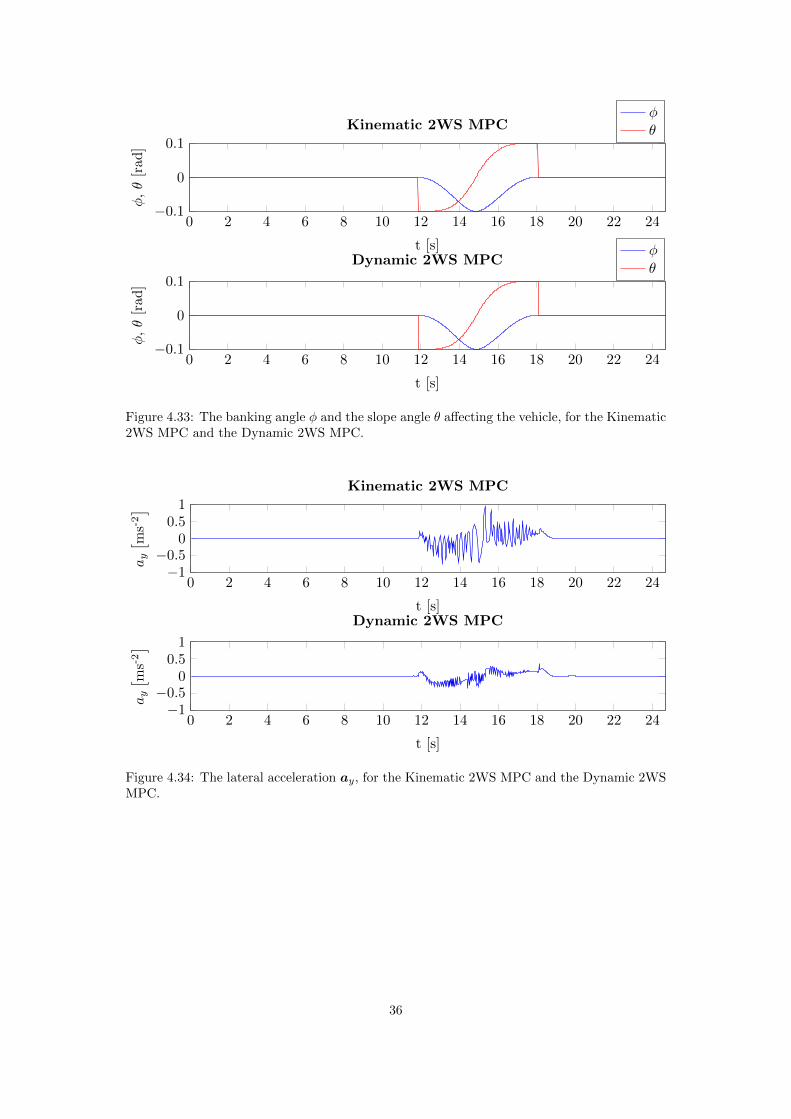
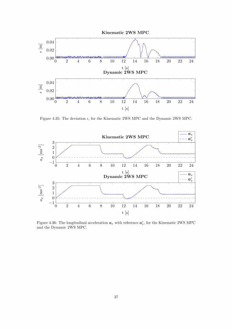
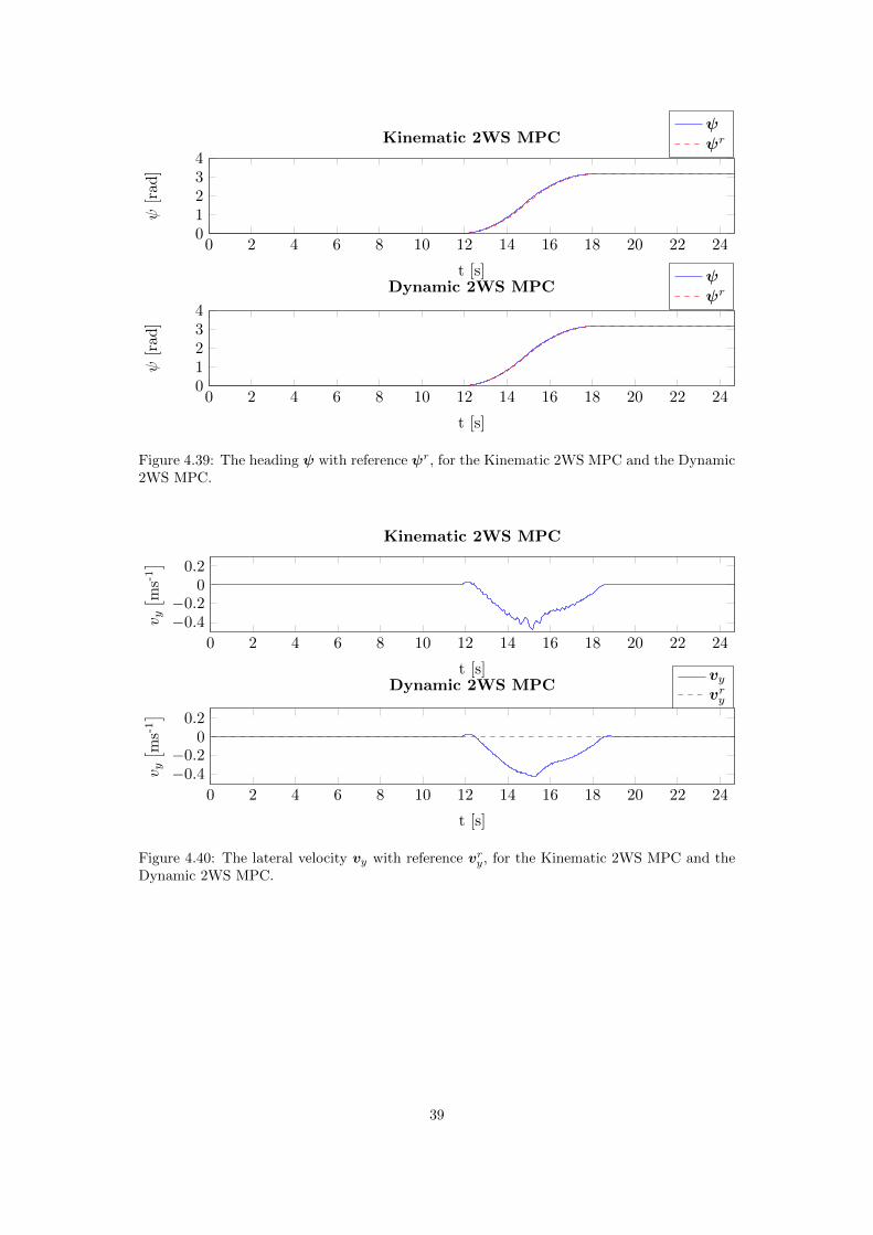
When making u-turn on a 10% downhill slope at 13.89 ms−1 (50 kph), seen the reference path[Xr,Y r], results in the driven path [X,Y ] which are displayed in Figure 4.32. The road slopeangle θ and the road bank angle φ affecting the vehicle depend on the heading of the vehiclein the turn, as shown in Figure 4.33. Compared to the same turn on a flat road the steeringangle change rate had to be increased to −0.12 ≤ ∆δf ≤ 0.12 rad/s. The maximum lateralacceleration ay reached is 0.94 ms−2, as shown in Figure 4.34, with a maximum deviation εof 0.05 m, shown in Figure 4.35. The MPC is tuned with the state and terminal state weightsQ = P = diag ([1, 100, 100, 100]), and the control input weights R = diag ([1, 1]), with statesin the same order as in (4.1), and the control inputs in the order ax first, and δf second.
34
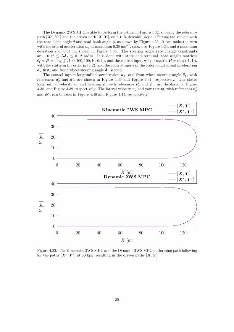
The Dynamic 2WS MPC is able to perform the u-turn in Figure 4.32, showing the referencepath [Xr,Y r] and the driven path [X,Y ], on a 10% downhill slope, affecting the vehicle withthe road slope angle θ and road bank angle φ, as shown by Figure 4.33. It can make the turnwith the lateral acceleration ay at maximum 0.38 ms−2, shown by Figure 4.34, and a maximumdeviation ε of 0.04 m, shown in Figure 4.35. The steering angle rate change constraintsare −0.12 ≤ ∆δf ≤ 0.12 rad/s. It is done with state and terminal state weight matricesQ = P = diag ([1, 100, 100, 100, 10, 0.1]), and the control input weight matrix R = diag ([1, 1]),with the states in the order in (4.2), and the control inputs in the order longitudinal accelerationax first, and front wheel steering angle δf second.
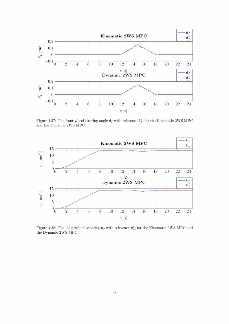
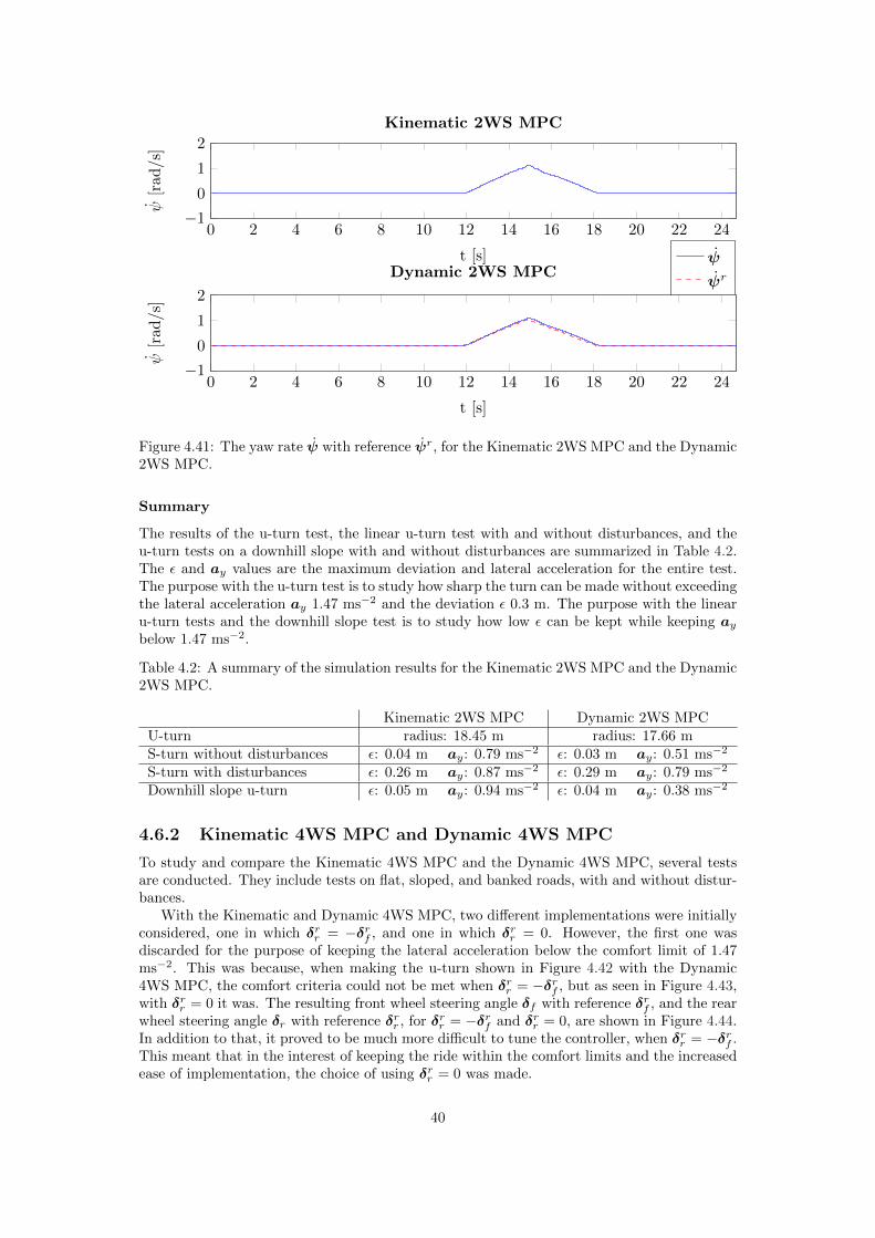
The control inputs longitudinal acceleration ax, and front wheel steering angle δf , withreferences arx and δrf , are shown in Figure 4.36 and Figure 4.37, respectively. The stateslongitudinal velocity vx and heading ψ, with references vrx and ψr, are displayed in Figure4.38, and Figure 4.39, respectively. The lateral velocity vy and yaw rate ψ, with references vryand ψr, can be seen in Figure 4.40 and Figure 4.41, respectively.
0 20 40 60 80 100 120
0
10
20
30
40
X [m]
Y[m
]
Kinematic 2WS MPC[X,Y ]
[Xr,Y r]
0 20 40 60 80 100 120
0
10
20
30
40
X [m]
Y[m
]
Dynamic 2WS MPC[X,Y ]
[Xr,Y r]
Figure 4.32: The Kinematic 2WS MPC and the Dynamic 2WS MPC performing path followingfor the paths [Xr,Y r] at 50 kph, resulting in the driven paths [X,Y ].
35
0 2 4 6 8 10 12 14 16 18 20 22 24−0.1
0
0.1
t [s]
φ,θ[rad]
Kinematic 2WS MPCφθ
0 2 4 6 8 10 12 14 16 18 20 22 24−0.1
0
0.1
t [s]
φ,θ[rad]
Dynamic 2WS MPCφθ
Figure 4.33: The banking angle φ and the slope angle θ affecting the vehicle, for the Kinematic2WS MPC and the Dynamic 2WS MPC.
0 2 4 6 8 10 12 14 16 18 20 22 24−1
−0.50
0.51
t [s]
ay
[ ms-2]
Kinematic 2WS MPC
0 2 4 6 8 10 12 14 16 18 20 22 24−1
−0.50
0.51
t [s]
ay
[ ms-2]
Dynamic 2WS MPC
Figure 4.34: The lateral acceleration ay, for the Kinematic 2WS MPC and the Dynamic 2WSMPC.
36
0 2 4 6 8 10 12 14 16 18 20 22 240.00
0.02
0.04
t [s]
ε[m
]
Kinematic 2WS MPC
0 2 4 6 8 10 12 14 16 18 20 22 240.00
0.02
0.04
t [s]
ε[m
]
Dynamic 2WS MPC
Figure 4.35: The deviation ε, for the Kinematic 2WS MPC and the Dynamic 2WS MPC.
0 2 4 6 8 10 12 14 16 18 20 22 24−10123
t [s]
ax
[ ms-2]
Kinematic 2WS MPCax
arx
0 2 4 6 8 10 12 14 16 18 20 22 24−10123
t [s]
ax
[ ms-2]
Dynamic 2WS MPCax
arx
Figure 4.36: The longitudinal acceleration ax with reference arx, for the Kinematic 2WS MPCand the Dynamic 2WS MPC.
37
0 2 4 6 8 10 12 14 16 18 20 22 24−0.1
0
0.1
0.2
t [s]
δ f[rad]
Kinematic 2WS MPCδfδrf
0 2 4 6 8 10 12 14 16 18 20 22 24−0.1
0
0.1
0.2
t [s]
δ f[rad]
Dynamic 2WS MPCδfδrf
Figure 4.37: The front wheel steering angle δf with reference δrf , for the Kinematic 2WS MPCand the Dynamic 2WS MPC.
0 2 4 6 8 10 12 14 16 18 20 22 240
5
10
15
t [s]
v x[ m
s-1]
Kinematic 2WS MPCvxvrx
0 2 4 6 8 10 12 14 16 18 20 22 240
5
10
15
t [s]
v x[ m
s-1]
Dynamic 2WS MPCvxvrx
Figure 4.38: The longitudinal velocity vx with reference vrx, for the Kinematic 2WS MPC andthe Dynamic 2WS MPC.
38
0 2 4 6 8 10 12 14 16 18 20 22 2401234
t [s]
ψ[rad]
Kinematic 2WS MPCψψr
0 2 4 6 8 10 12 14 16 18 20 22 2401234
t [s]
ψ[rad]
Dynamic 2WS MPCψψr
Figure 4.39: The heading ψ with reference ψr, for the Kinematic 2WS MPC and the Dynamic2WS MPC.
0 2 4 6 8 10 12 14 16 18 20 22 24
−0.4−0.2
00.2
t [s]
v y[ m
s-1]
Kinematic 2WS MPC
0 2 4 6 8 10 12 14 16 18 20 22 24
−0.4−0.2
00.2
t [s]
v y[ m
s-1]
Dynamic 2WS MPCvyvry
Figure 4.40: The lateral velocity vy with reference vry, for the Kinematic 2WS MPC and theDynamic 2WS MPC.
39
0 2 4 6 8 10 12 14 16 18 20 22 24−1
0
1
2
t [s]
ψ[rad/s]
Kinematic 2WS MPC
0 2 4 6 8 10 12 14 16 18 20 22 24−1
0
1
2
t [s]
ψ[rad/s]
Dynamic 2WS MPCψ
ψr
Figure 4.41: The yaw rate ψ with reference ψr, for the Kinematic 2WS MPC and the Dynamic2WS MPC.
Summary
The results of the u-turn test, the linear u-turn test with and without disturbances, and theu-turn tests on a downhill slope with and without disturbances are summarized in Table 4.2.The ε and ay values are the maximum deviation and lateral acceleration for the entire test.The purpose with the u-turn test is to study how sharp the turn can be made without exceedingthe lateral acceleration ay 1.47 ms−2 and the deviation ε 0.3 m. The purpose with the linearu-turn tests and the downhill slope test is to study how low ε can be kept while keeping aybelow 1.47 ms−2.
Table 4.2: A summary of the simulation results for the Kinematic 2WS MPC and the Dynamic2WS MPC.
Kinematic 2WS MPC Dynamic 2WS MPCU-turn radius: 18.45 m radius: 17.66 mS-turn without disturbances ε: 0.04 m ay: 0.79 ms−2 ε: 0.03 m ay: 0.51 ms−2
S-turn with disturbances ε: 0.26 m ay: 0.87 ms−2 ε: 0.29 m ay: 0.79 ms−2
Downhill slope u-turn ε: 0.05 m ay: 0.94 ms−2 ε: 0.04 m ay: 0.38 ms−2
4.6.2 Kinematic 4WS MPC and Dynamic 4WS MPC
To study and compare the Kinematic 4WS MPC and the Dynamic 4WS MPC, several testsare conducted. They include tests on flat, sloped, and banked roads, with and without distur-bances.
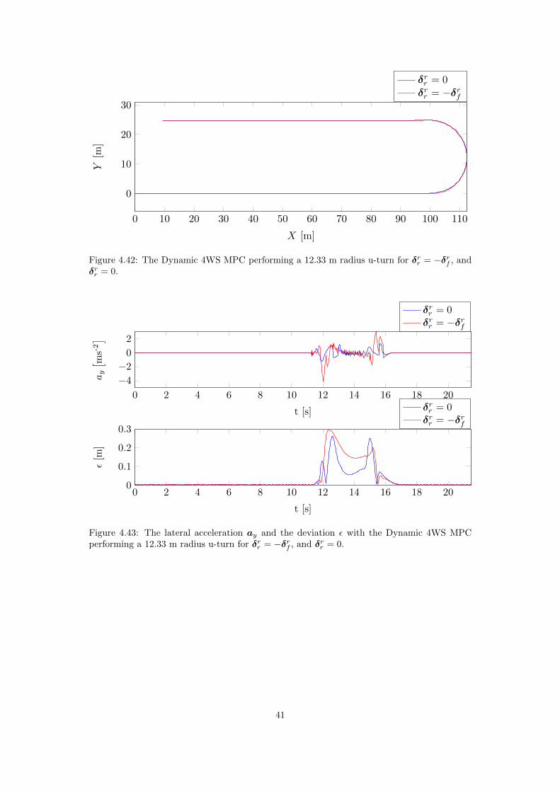
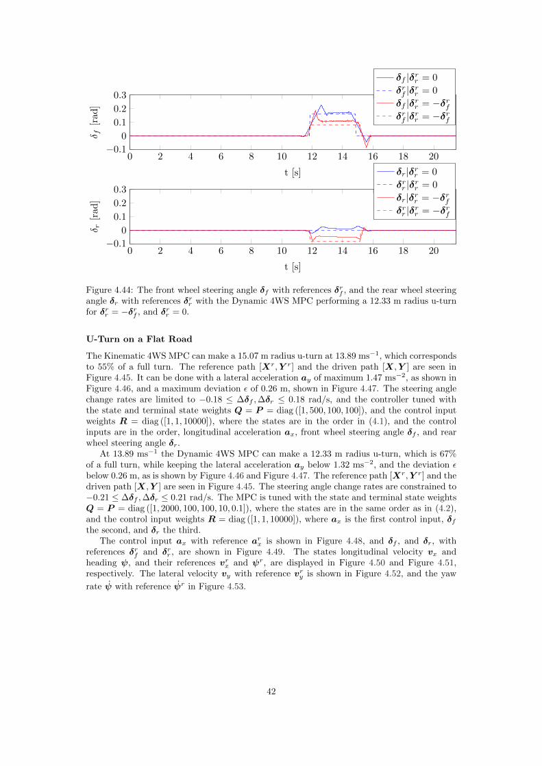
With the Kinematic and Dynamic 4WS MPC, two different implementations were initiallyconsidered, one in which δrr = −δrf , and one in which δrr = 0. However, the first one wasdiscarded for the purpose of keeping the lateral acceleration below the comfort limit of 1.47ms−2. This was because, when making the u-turn shown in Figure 4.42 with the Dynamic4WS MPC, the comfort criteria could not be met when δrr = −δrf , but as seen in Figure 4.43,with δrr = 0 it was. The resulting front wheel steering angle δf with reference δrf , and the rearwheel steering angle δr with reference δrr , for δrr = −δrf and δrr = 0, are shown in Figure 4.44.In addition to that, it proved to be much more difficult to tune the controller, when δrr = −δrf .This meant that in the interest of keeping the ride within the comfort limits and the increasedease of implementation, the choice of using δrr = 0 was made.
40
0 10 20 30 40 50 60 70 80 90 100 110
0
10
20
30
X [m]
Y[m
]
δrr = 0δrr = −δrf
Figure 4.42: The Dynamic 4WS MPC performing a 12.33 m radius u-turn for δrr = −δrf , andδrr = 0.
0 2 4 6 8 10 12 14 16 18 20
−4
−2
0
2
t [s]
ay
[ ms-2]
δrr = 0δrr = −δrf
0 2 4 6 8 10 12 14 16 18 200
0.1
0.2
0.3
t [s]
ε[m
]
δrr = 0δrr = −δrf
Figure 4.43: The lateral acceleration ay and the deviation ε with the Dynamic 4WS MPCperforming a 12.33 m radius u-turn for δrr = −δrf , and δrr = 0.
41
0 2 4 6 8 10 12 14 16 18 20−0.1
0
0.1
0.2
0.3
t [s]
δ f[rad]
δf |δrr = 0
δrf |δrr = 0
δf |δrr = −δrfδrf |δrr = −δrf
0 2 4 6 8 10 12 14 16 18 20−0.1
0
0.1
0.2
0.3
t [s]
δ r[rad
]
δr|δrr = 0
δrr |δrr = 0
δr|δrr = −δrfδrr |δrr = −δrf
Figure 4.44: The front wheel steering angle δf with references δrf , and the rear wheel steeringangle δr with references δrr with the Dynamic 4WS MPC performing a 12.33 m radius u-turnfor δrr = −δrf , and δrr = 0.
U-Turn on a Flat Road
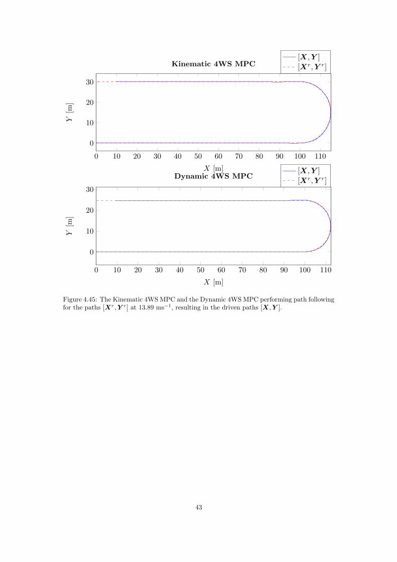
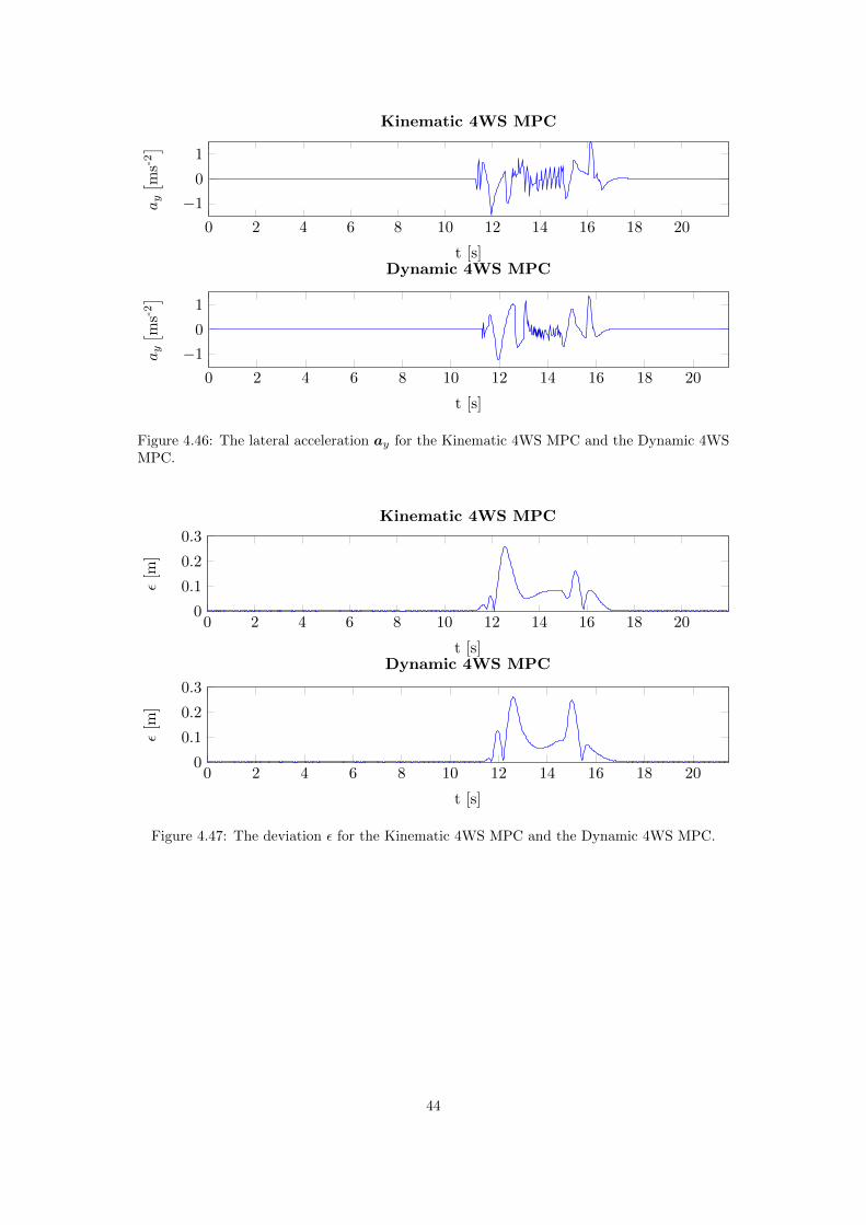
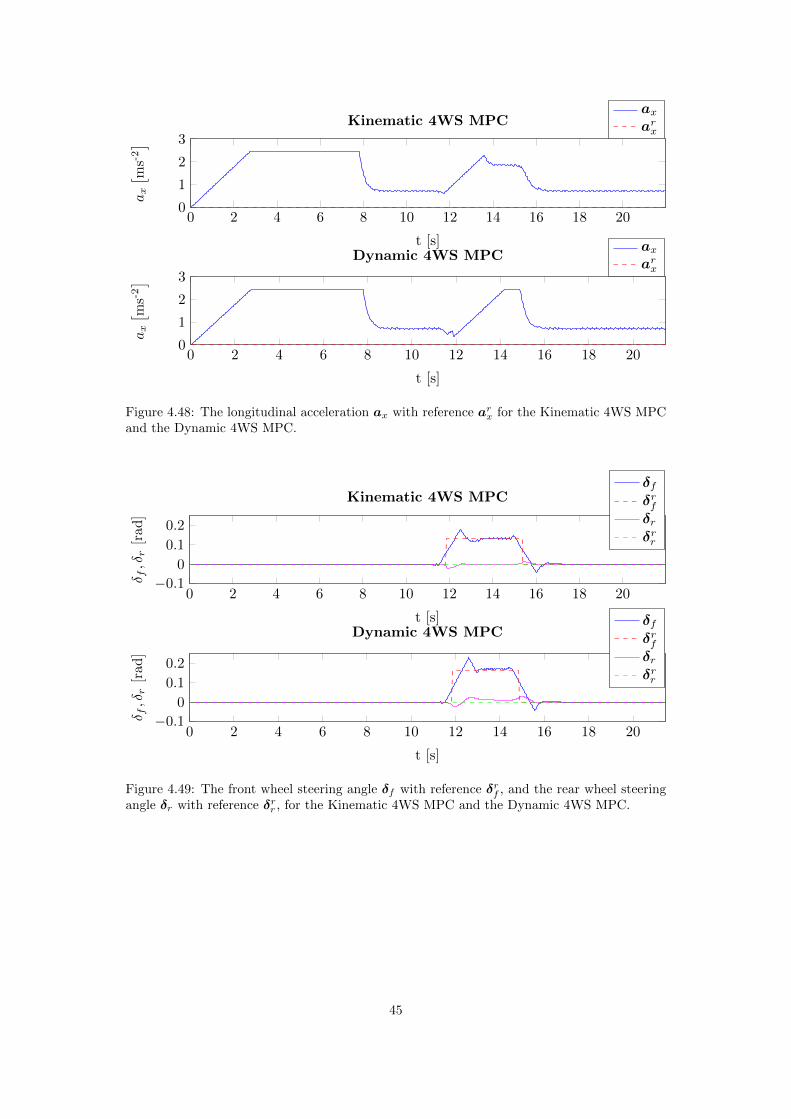
The Kinematic 4WS MPC can make a 15.07 m radius u-turn at 13.89 ms−1, which correspondsto 55% of a full turn. The reference path [Xr,Y r] and the driven path [X,Y ] are seen inFigure 4.45. It can be done with a lateral acceleration ay of maximum 1.47 ms−2, as shown inFigure 4.46, and a maximum deviation ε of 0.26 m, shown in Figure 4.47. The steering anglechange rates are limited to −0.18 ≤ ∆δf ,∆δr ≤ 0.18 rad/s, and the controller tuned withthe state and terminal state weights Q = P = diag ([1, 500, 100, 100]), and the control inputweights R = diag ([1, 1, 10000]), where the states are in the order in (4.1), and the controlinputs are in the order, longitudinal acceleration ax, front wheel steering angle δf , and rearwheel steering angle δr.
At 13.89 ms−1 the Dynamic 4WS MPC can make a 12.33 m radius u-turn, which is 67%of a full turn, while keeping the lateral acceleration ay below 1.32 ms−2, and the deviation εbelow 0.26 m, as is shown by Figure 4.46 and Figure 4.47. The reference path [Xr,Y r] and thedriven path [X,Y ] are seen in Figure 4.45. The steering angle change rates are constrained to−0.21 ≤ ∆δf ,∆δr ≤ 0.21 rad/s. The MPC is tuned with the state and terminal state weightsQ = P = diag ([1, 2000, 100, 100, 10, 0.1]), where the states are in the same order as in (4.2),and the control input weights R = diag ([1, 1, 10000]), where ax is the first control input, δfthe second, and δr the third.
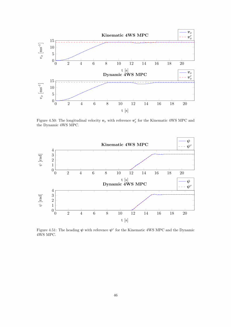
The control input ax with reference arx is shown in Figure 4.48, and δf , and δr, withreferences δrf and δrr , are shown in Figure 4.49. The states longitudinal velocity vx andheading ψ, and their references vrx and ψr, are displayed in Figure 4.50 and Figure 4.51,respectively. The lateral velocity vy with reference vry is shown in Figure 4.52, and the yaw
rate ψ with reference ψr in Figure 4.53.
42
0 10 20 30 40 50 60 70 80 90 100 110
0
10
20
30
X [m]
Y[m
]
Dynamic 4WS MPC[X,Y ]
[Xr,Y r]
0 10 20 30 40 50 60 70 80 90 100 110
0
10
20
30
X [m]
Y[m
]Kinematic 4WS MPC
[X,Y ]
[Xr,Y r]
Figure 4.45: The Kinematic 4WS MPC and the Dynamic 4WS MPC performing path followingfor the paths [Xr,Y r] at 13.89 ms−1, resulting in the driven paths [X,Y ].
43
0 2 4 6 8 10 12 14 16 18 20
−1
0
1
t [s]
ay
[ ms-2]
Kinematic 4WS MPC
0 2 4 6 8 10 12 14 16 18 20
−1
0
1
t [s]
ay
[ ms-2]
Dynamic 4WS MPC
Figure 4.46: The lateral acceleration ay for the Kinematic 4WS MPC and the Dynamic 4WSMPC.
0 2 4 6 8 10 12 14 16 18 200
0.1
0.2
0.3
t [s]
ε[m
]
Kinematic 4WS MPC
0 2 4 6 8 10 12 14 16 18 200
0.1
0.2
0.3
t [s]
ε[m
]
Dynamic 4WS MPC
Figure 4.47: The deviation ε for the Kinematic 4WS MPC and the Dynamic 4WS MPC.
44
0 2 4 6 8 10 12 14 16 18 200
1
2
3
t [s]
ax
[ ms-2]
Kinematic 4WS MPCax
arx
0 2 4 6 8 10 12 14 16 18 200
1
2
3
t [s]
ax
[ ms-2]
Dynamic 4WS MPCax
arx
Figure 4.48: The longitudinal acceleration ax with reference arx for the Kinematic 4WS MPCand the Dynamic 4WS MPC.
0 2 4 6 8 10 12 14 16 18 20−0.1
0
0.1
0.2
t [s]
δ f,δ
r[rad
]
Kinematic 4WS MPCδfδrfδrδrr
0 2 4 6 8 10 12 14 16 18 20−0.1
0
0.1
0.2
t [s]
δ f,δ
r[rad
]
Dynamic 4WS MPCδfδrfδrδrr
Figure 4.49: The front wheel steering angle δf with reference δrf , and the rear wheel steeringangle δr with reference δrr , for the Kinematic 4WS MPC and the Dynamic 4WS MPC.
45
0 2 4 6 8 10 12 14 16 18 200
5
10
15
t [s]
v x[ m
s-1]
Kinematic 4WS MPCvxvrx
0 2 4 6 8 10 12 14 16 18 200
5
10
15
t [s]
v x[ m
s-1]
Dynamic 4WS MPCvxvrx
Figure 4.50: The longitudinal velocity vx with reference vrx for the Kinematic 4WS MPC andthe Dynamic 4WS MPC.
0 2 4 6 8 10 12 14 16 18 2001234
t [s]
ψ[rad]
Kinematic 4WS MPCψψr
0 2 4 6 8 10 12 14 16 18 2001234
t [s]
ψ[rad
]
Dynamic 4WS MPCψψr
Figure 4.51: The heading ψ with reference ψr for the Kinematic 4WS MPC and the Dynamic4WS MPC.
46
0 2 4 6 8 10 12 14 16 18 20
−0.4
−0.2
0
0.2
t [s]
v y[ m
s-1]
Kinematic 4WS MPC
0 2 4 6 8 10 12 14 16 18 20
−0.4
−0.2
0
0.2
t [s]
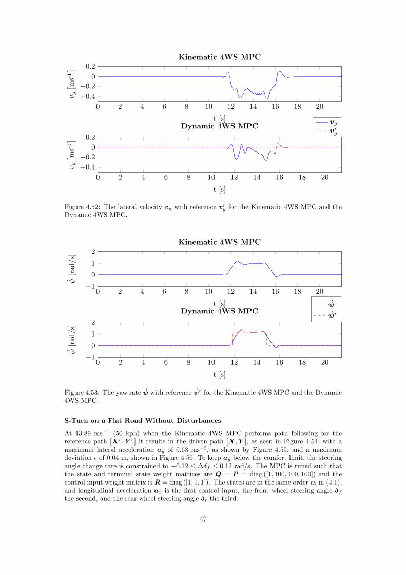
v y[ m
s-1]
Dynamic 4WS MPCvyvry
Figure 4.52: The lateral velocity vy with reference vry for the Kinematic 4WS MPC and theDynamic 4WS MPC.
0 2 4 6 8 10 12 14 16 18 20−1
0
1
2
t [s]
ψ[rad
/s]
Kinematic 4WS MPC
0 2 4 6 8 10 12 14 16 18 20−1
0
1
2
t [s]
ψ[rad
/s]
Dynamic 4WS MPCψ
ψr
Figure 4.53: The yaw rate ψ with reference ψr for the Kinematic 4WS MPC and the Dynamic4WS MPC.
S-Turn on a Flat Road Without Disturbances
At 13.89 ms−1 (50 kph) when the Kinematic 4WS MPC performs path following for thereference path [Xr,Y r] it results in the driven path [X,Y ], as seen in Figure 4.54, with amaximum lateral acceleration ay of 0.63 ms−2, as shown by Figure 4.55, and a maximumdeviation ε of 0.04 m, shown in Figure 4.56. To keep ay below the comfort limit, the steeringangle change rate is constrained to −0.12 ≤ ∆δf ≤ 0.12 rad/s. The MPC is tuned such thatthe state and terminal state weight matrices are Q = P = diag ([1, 100, 100, 100]) and thecontrol input weight matrix is R = diag ([1, 1, 1]). The states are in the same order as in (4.1),and longitudinal acceleration ax is the first control input, the front wheel steering angle δfthe second, and the rear wheel steering angle δr the third.
47
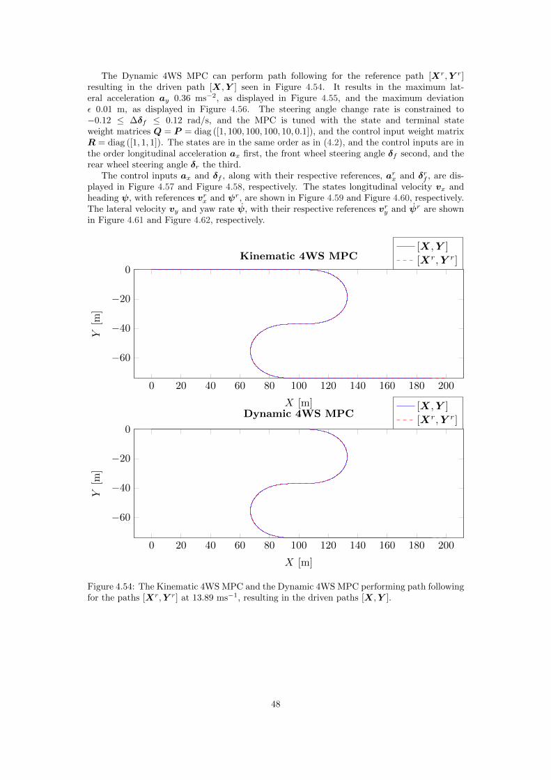
The Dynamic 4WS MPC can perform path following for the reference path [Xr,Y r]resulting in the driven path [X,Y ] seen in Figure 4.54. It results in the maximum lat-eral acceleration ay 0.36 ms−2, as displayed in Figure 4.55, and the maximum deviationε 0.01 m, as displayed in Figure 4.56. The steering angle change rate is constrained to−0.12 ≤ ∆δf ≤ 0.12 rad/s, and the MPC is tuned with the state and terminal stateweight matrices Q = P = diag ([1, 100, 100, 100, 10, 0.1]), and the control input weight matrixR = diag ([1, 1, 1]). The states are in the same order as in (4.2), and the control inputs are inthe order longitudinal acceleration ax first, the front wheel steering angle δf second, and therear wheel steering angle δr the third.
The control inputs ax and δf , along with their respective references, arx and δrf , are dis-played in Figure 4.57 and Figure 4.58, respectively. The states longitudinal velocity vx andheading ψ, with references vrx and ψr, are shown in Figure 4.59 and Figure 4.60, respectively.The lateral velocity vy and yaw rate ψ, with their respective references vry and ψr are shownin Figure 4.61 and Figure 4.62, respectively.
0 20 40 60 80 100 120 140 160 180 200
−60
−40
−20
0
X [m]
Y[m
]
Kinematic 4WS MPC[X,Y ]
[Xr,Y r]
0 20 40 60 80 100 120 140 160 180 200
−60
−40
−20
0
X [m]
Y[m
]
Dynamic 4WS MPC[X,Y ]
[Xr,Y r]
Figure 4.54: The Kinematic 4WS MPC and the Dynamic 4WS MPC performing path followingfor the paths [Xr,Y r] at 13.89 ms−1, resulting in the driven paths [X,Y ].
48
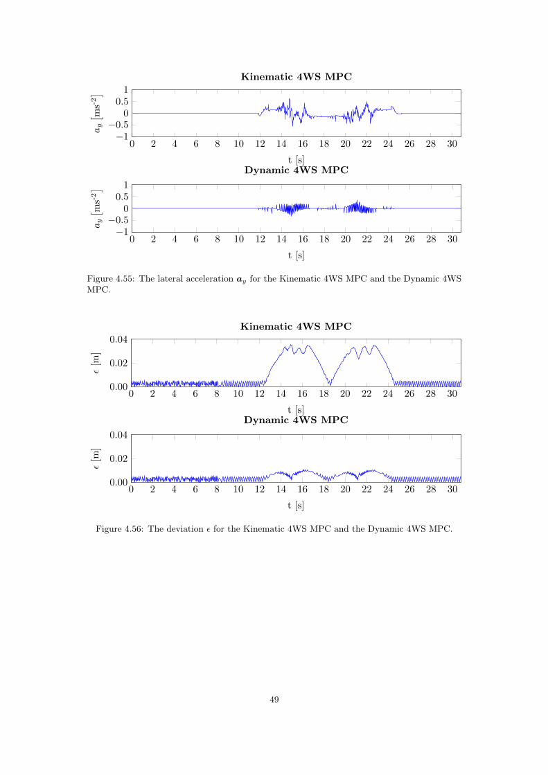
0 2 4 6 8 10 12 14 16 18 20 22 24 26 28 30−1
−0.50
0.51
t [s]
ay
[ ms-2]
Kinematic 4WS MPC
0 2 4 6 8 10 12 14 16 18 20 22 24 26 28 30−1
−0.50
0.51
t [s]
ay
[ ms-2]
Dynamic 4WS MPC
Figure 4.55: The lateral acceleration ay for the Kinematic 4WS MPC and the Dynamic 4WSMPC.
0 2 4 6 8 10 12 14 16 18 20 22 24 26 28 300.00
0.02
0.04
t [s]
ε[m
]
Kinematic 4WS MPC
0 2 4 6 8 10 12 14 16 18 20 22 24 26 28 300.00
0.02
0.04
t [s]
ε[m
]
Dynamic 4WS MPC
Figure 4.56: The deviation ε for the Kinematic 4WS MPC and the Dynamic 4WS MPC.
49
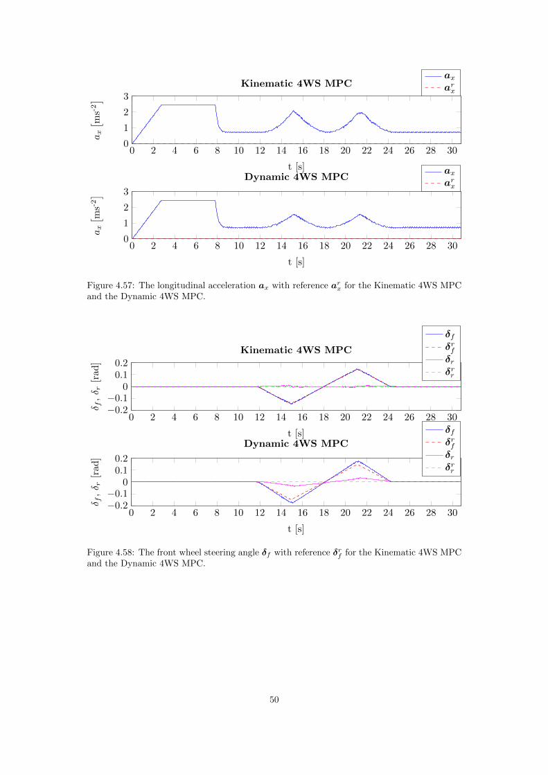
0 2 4 6 8 10 12 14 16 18 20 22 24 26 28 300
1
2
3
t [s]
ax
[ ms-2]
Kinematic 4WS MPCax
arx
0 2 4 6 8 10 12 14 16 18 20 22 24 26 28 300
1
2
3
t [s]
ax
[ ms-2]
Dynamic 4WS MPCax
arx
Figure 4.57: The longitudinal acceleration ax with reference arx for the Kinematic 4WS MPCand the Dynamic 4WS MPC.
0 2 4 6 8 10 12 14 16 18 20 22 24 26 28 30−0.2−0.1
00.10.2
t [s]
δ f,δ r
[rad
]
Kinematic 4WS MPC
δfδrfδrδrr
0 2 4 6 8 10 12 14 16 18 20 22 24 26 28 30−0.2−0.1
00.10.2
t [s]
δ f,δ r
[rad
]
Dynamic 4WS MPC
δfδrfδrδrr
Figure 4.58: The front wheel steering angle δf with reference δrf for the Kinematic 4WS MPCand the Dynamic 4WS MPC.
50

0 2 4 6 8 10 12 14 16 18 20 22 24 26 28 300
5
10
15
t [s]
v x[ m
s-1]
Kinematic 4WS MPCvxvrx
0 2 4 6 8 10 12 14 16 18 20 22 24 26 28 300
5
10
15
t [s]
v x[ m
s-1]
Dynamic 4WS MPCvxvrx
Figure 4.59: The longitudinal velocity vx with reference vrx for the Kinematic 4WS MPC andthe Dynamic 4WS MPC.
0 2 4 6 8 10 12 14 16 18 20 22 24 26 28 30−4
−2
0
t [s]
ψ[rad]
Kinematic 4WS MPCψψr
0 2 4 6 8 10 12 14 16 18 20 22 24 26 28 30−4
−2
0
t [s]
ψ[rad]
Dynamic 4WS MPCψψr
Figure 4.60: The heading ψ with reference ψr for the Kinematic 4WS MPC and the Dynamic4WS MPC.
51
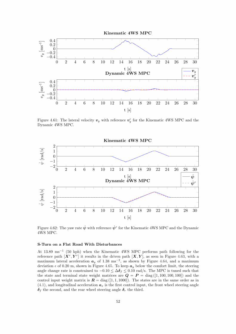
0 2 4 6 8 10 12 14 16 18 20 22 24 26 28 30−0.4−0.2
00.20.4
t [s]
v y[ m
s-1]
Kinematic 4WS MPC
0 2 4 6 8 10 12 14 16 18 20 22 24 26 28 30−0.4−0.2
00.20.4
t [s]
v y[ m
s-1]
Dynamic 4WS MPCvyvry
Figure 4.61: The lateral velocity vy with reference vry for the Kinematic 4WS MPC and theDynamic 4WS MPC.
0 2 4 6 8 10 12 14 16 18 20 22 24 26 28 30−2−1012
t [s]
ψ[rad
/s]
Kinematic 4WS MPC
0 2 4 6 8 10 12 14 16 18 20 22 24 26 28 30−2−1012
t [s]
ψ[rad
/s]
Dynamic 4WS MPCψ
ψr
Figure 4.62: The yaw rate ψ with reference ψr for the Kinematic 4WS MPC and the Dynamic4WS MPC.
S-Turn on a Flat Road With Disturbances
At 13.89 ms−1 (50 kph) when the Kinematic 4WS MPC performs path following for thereference path [Xr,Y r] it results in the driven path [X,Y ], as seen in Figure 4.63, with amaximum lateral acceleration ay of 1.38 ms−2, as shown by Figure 4.64, and a maximumdeviation ε of 0.20 m, shown in Figure 4.65. To keep ay below the comfort limit, the steeringangle change rate is constrained to −0.10 ≤ ∆δf ≤ 0.10 rad/s. The MPC is tuned such thatthe state and terminal state weight matrices are Q = P = diag ([1, 100, 100, 100]) and thecontrol input weight matrix is R = diag ([1, 1, 1000]). The states are in the same order as in(4.1), and longitudinal acceleration ax is the first control input, the front wheel steering angleδf the second, and the rear wheel steering angle δr the third.
52
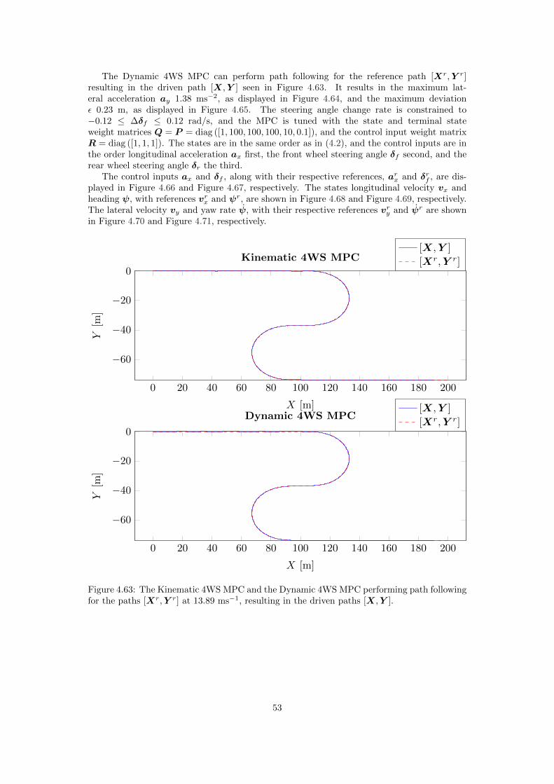
The Dynamic 4WS MPC can perform path following for the reference path [Xr,Y r]resulting in the driven path [X,Y ] seen in Figure 4.63. It results in the maximum lat-eral acceleration ay 1.38 ms−2, as displayed in Figure 4.64, and the maximum deviationε 0.23 m, as displayed in Figure 4.65. The steering angle change rate is constrained to−0.12 ≤ ∆δf ≤ 0.12 rad/s, and the MPC is tuned with the state and terminal stateweight matrices Q = P = diag ([1, 100, 100, 100, 10, 0.1]), and the control input weight matrixR = diag ([1, 1, 1]). The states are in the same order as in (4.2), and the control inputs are inthe order longitudinal acceleration ax first, the front wheel steering angle δf second, and therear wheel steering angle δr the third.
The control inputs ax and δf , along with their respective references, arx and δrf , are dis-played in Figure 4.66 and Figure 4.67, respectively. The states longitudinal velocity vx andheading ψ, with references vrx and ψr, are shown in Figure 4.68 and Figure 4.69, respectively.The lateral velocity vy and yaw rate ψ, with their respective references vry and ψr are shownin Figure 4.70 and Figure 4.71, respectively.
0 20 40 60 80 100 120 140 160 180 200
−60
−40
−20
0
X [m]
Y[m
]
Kinematic 4WS MPC[X,Y ]
[Xr,Y r]
0 20 40 60 80 100 120 140 160 180 200
−60
−40
−20
0
X [m]
Y[m
]
Dynamic 4WS MPC[X,Y ]
[Xr,Y r]
Figure 4.63: The Kinematic 4WS MPC and the Dynamic 4WS MPC performing path followingfor the paths [Xr,Y r] at 13.89 ms−1, resulting in the driven paths [X,Y ].
53
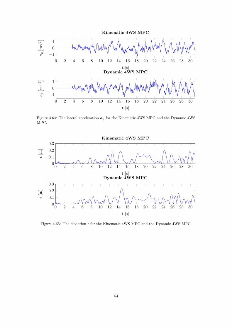
0 2 4 6 8 10 12 14 16 18 20 22 24 26 28 30
−1
0
1
t [s]
ay
[ ms-2]
Kinematic 4WS MPC
0 2 4 6 8 10 12 14 16 18 20 22 24 26 28 30
−1
0
1
t [s]
ay
[ ms-2]
Dynamic 4WS MPC
Figure 4.64: The lateral acceleration ay for the Kinematic 4WS MPC and the Dynamic 4WSMPC.
0 2 4 6 8 10 12 14 16 18 20 22 24 26 28 300
0.1
0.2
0.3
t [s]
ε[m
]
Kinematic 4WS MPC
0 2 4 6 8 10 12 14 16 18 20 22 24 26 28 300
0.1
0.2
0.3
t [s]
ε[m
]
Dynamic 4WS MPC
Figure 4.65: The deviation ε for the Kinematic 4WS MPC and the Dynamic 4WS MPC.
54
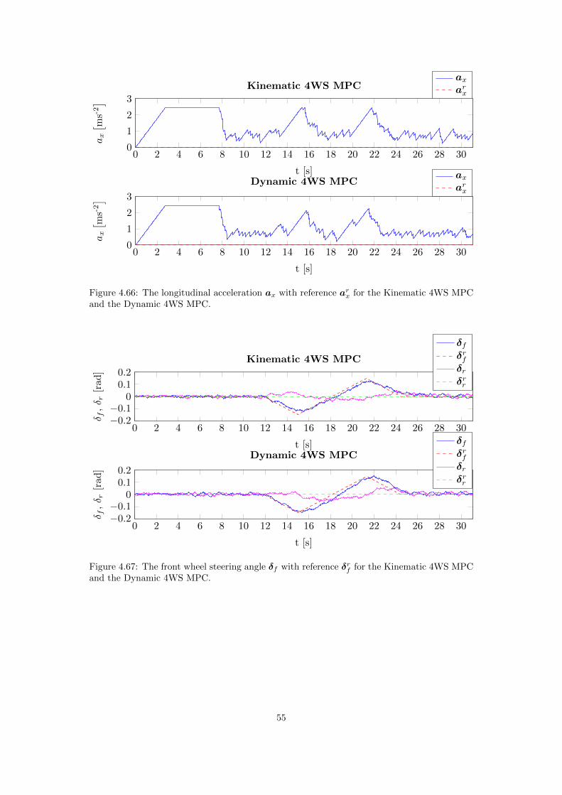
0 2 4 6 8 10 12 14 16 18 20 22 24 26 28 300
1
2
3
t [s]
ax
[ ms-2]
Kinematic 4WS MPCax
arx
0 2 4 6 8 10 12 14 16 18 20 22 24 26 28 300
1
2
3
t [s]
ax
[ ms-2]
Dynamic 4WS MPCax
arx
Figure 4.66: The longitudinal acceleration ax with reference arx for the Kinematic 4WS MPCand the Dynamic 4WS MPC.
0 2 4 6 8 10 12 14 16 18 20 22 24 26 28 30−0.2−0.1
00.10.2
t [s]
δ f,δ r
[rad
]
Kinematic 4WS MPC
δfδrfδrδrr
0 2 4 6 8 10 12 14 16 18 20 22 24 26 28 30−0.2−0.1
00.10.2
t [s]
δ f,δ r
[rad
]
Dynamic 4WS MPC
δfδrfδrδrr
Figure 4.67: The front wheel steering angle δf with reference δrf for the Kinematic 4WS MPCand the Dynamic 4WS MPC.
55
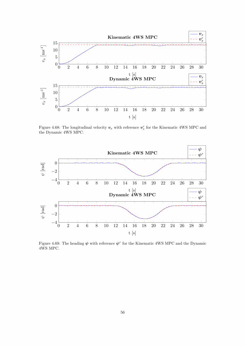
0 2 4 6 8 10 12 14 16 18 20 22 24 26 28 300
5
10
15
t [s]
v x[ m
s-1]
Kinematic 4WS MPCvxvrx
0 2 4 6 8 10 12 14 16 18 20 22 24 26 28 300
5
10
15
t [s]
v x[ m
s-1]
Dynamic 4WS MPCvxvrx
Figure 4.68: The longitudinal velocity vx with reference vrx for the Kinematic 4WS MPC andthe Dynamic 4WS MPC.
0 2 4 6 8 10 12 14 16 18 20 22 24 26 28 30−4
−2
0
t [s]
ψ[rad]
Kinematic 4WS MPCψψr
0 2 4 6 8 10 12 14 16 18 20 22 24 26 28 30−4
−2
0
t [s]
ψ[rad]
Dynamic 4WS MPCψψr
Figure 4.69: The heading ψ with reference ψr for the Kinematic 4WS MPC and the Dynamic4WS MPC.
56
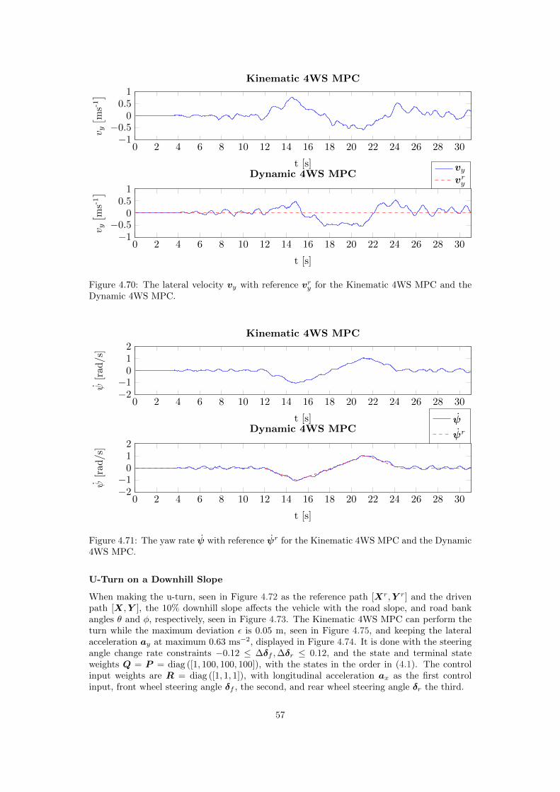
0 2 4 6 8 10 12 14 16 18 20 22 24 26 28 30−1
−0.50
0.51
t [s]
v y[ m
s-1]
Kinematic 4WS MPC
0 2 4 6 8 10 12 14 16 18 20 22 24 26 28 30−1
−0.50
0.51
t [s]
v y[ m
s-1]
Dynamic 4WS MPCvyvry
Figure 4.70: The lateral velocity vy with reference vry for the Kinematic 4WS MPC and theDynamic 4WS MPC.
0 2 4 6 8 10 12 14 16 18 20 22 24 26 28 30−2−1012
t [s]
ψ[rad
/s]
Kinematic 4WS MPC
0 2 4 6 8 10 12 14 16 18 20 22 24 26 28 30−2−1012
t [s]
ψ[rad
/s]
Dynamic 4WS MPCψ
ψr
Figure 4.71: The yaw rate ψ with reference ψr for the Kinematic 4WS MPC and the Dynamic4WS MPC.
U-Turn on a Downhill Slope
When making the u-turn, seen in Figure 4.72 as the reference path [Xr,Y r] and the drivenpath [X,Y ], the 10% downhill slope affects the vehicle with the road slope, and road bankangles θ and φ, respectively, seen in Figure 4.73. The Kinematic 4WS MPC can perform theturn while the maximum deviation ε is 0.05 m, seen in Figure 4.75, and keeping the lateralacceleration ay at maximum 0.63 ms−2, displayed in Figure 4.74. It is done with the steeringangle change rate constraints −0.12 ≤ ∆δf ,∆δr ≤ 0.12, and the state and terminal stateweights Q = P = diag ([1, 100, 100, 100]), with the states in the order in (4.1). The controlinput weights are R = diag ([1, 1, 1]), with longitudinal acceleration ax as the first controlinput, front wheel steering angle δf , the second, and rear wheel steering angle δr the third.
57
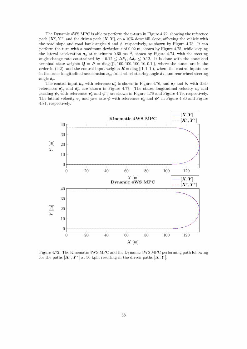
The Dynamic 4WS MPC is able to perform the u-turn in Figure 4.72, showing the referencepath [Xr,Y r] and the driven path [X,Y ], on a 10% downhill slope, affecting the vehicle withthe road slope and road bank angles θ and φ, respectively, as shown by Figure 4.73. It canperform the turn with a maximum deviation ε of 0.02 m, shown by Figure 4.75, while keepingthe lateral acceleration ay at maximum 0.60 ms−2, shown by Figure 4.74, with the steeringangle change rate constrained by −0.12 ≤ ∆δf ,∆δr ≤ 0.12. It is done with the state andterminal state weights Q = P = diag ([1, 100, 100, 100, 10, 0.1]), where the states are in theorder in (4.2), and the control input weights R = diag ([1, 1, 1]), where the control inputs arein the order longitudinal acceleration ax, front wheel steering angle δf , and rear wheel steeringangle δr.
The control input ax with reference arx is shown in Figure 4.76, and δf and δr with theirreferences δrf , and δrr , are shown in Figure 4.77. The states longitudinal velocity vx andheading ψ, with references vrx and ψr, are shown in Figure 4.78 and Figure 4.79, respectively.The lateral velocity vy and yaw rate ψ with references vry and ψr in Figure 4.80 and Figure4.81, respectively.
0 20 40 60 80 100 120
0
10
20
30
40
X [m]
Y[m
]
Kinematic 4WS MPC[X,Y ]
[Xr,Y r]
0 20 40 60 80 100 120
0
10
20
30
40
X [m]
Y[m
]
Dynamic 4WS MPC[X,Y ]
[Xr,Y r]
Figure 4.72: The Kinematic 4WS MPC and the Dynamic 4WS MPC performing path followingfor the paths [Xr,Y r] at 50 kph, resulting in the driven paths [X,Y ].
58
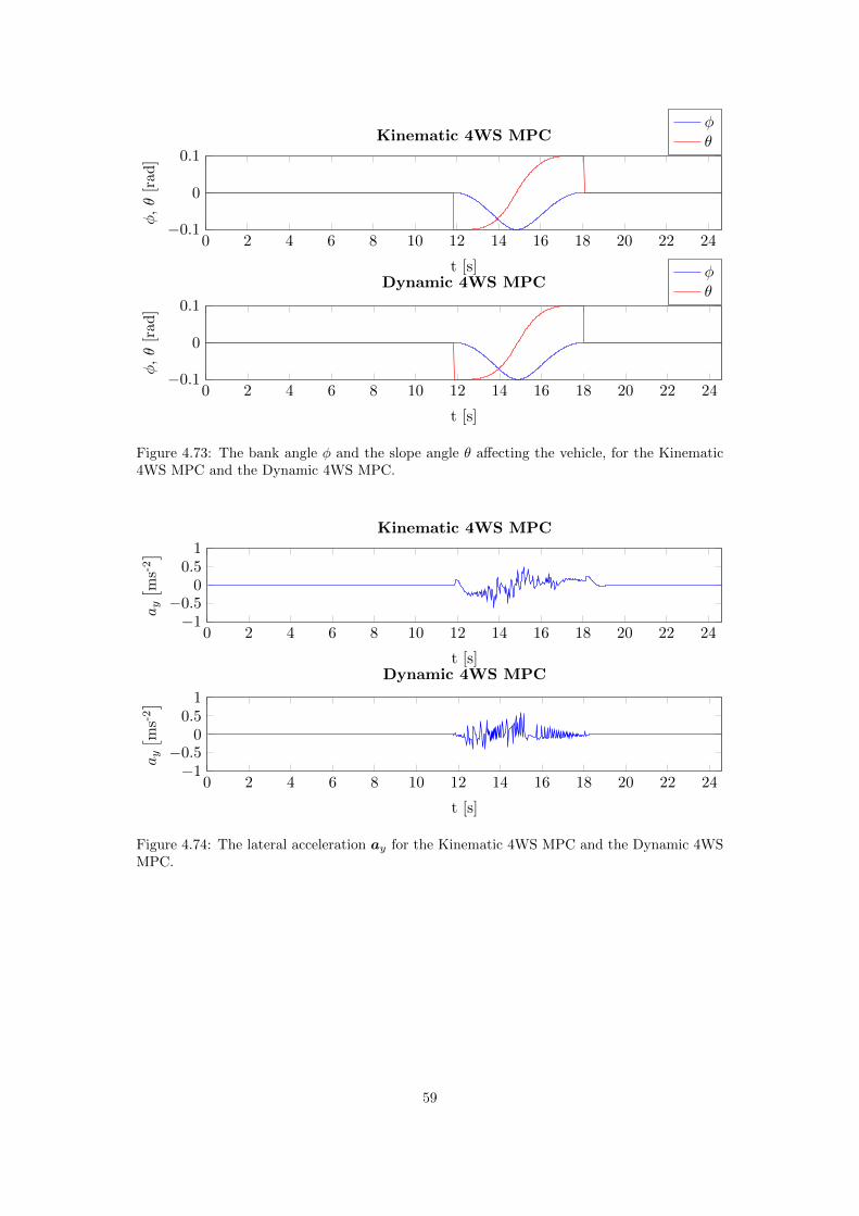
0 2 4 6 8 10 12 14 16 18 20 22 24−0.1
0
0.1
t [s]
φ,θ[rad
]Kinematic 4WS MPC
φθ
0 2 4 6 8 10 12 14 16 18 20 22 24−0.1
0
0.1
t [s]
φ,θ[rad
]
Dynamic 4WS MPCφθ
Figure 4.73: The bank angle φ and the slope angle θ affecting the vehicle, for the Kinematic4WS MPC and the Dynamic 4WS MPC.
0 2 4 6 8 10 12 14 16 18 20 22 24−1
−0.50
0.51
t [s]
ay
[ ms-2]
Kinematic 4WS MPC
0 2 4 6 8 10 12 14 16 18 20 22 24−1
−0.50
0.51
t [s]
ay
[ ms-2]
Dynamic 4WS MPC
Figure 4.74: The lateral acceleration ay for the Kinematic 4WS MPC and the Dynamic 4WSMPC.
59
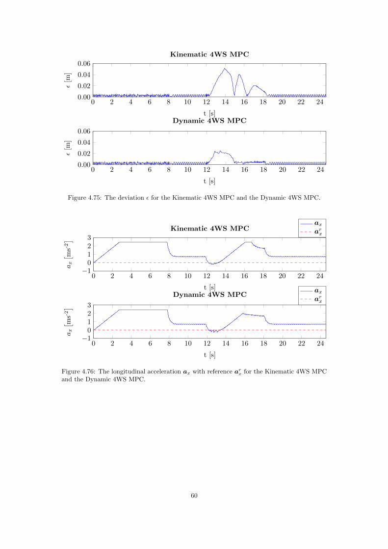
0 2 4 6 8 10 12 14 16 18 20 22 240.00
0.02
0.04
0.06
t [s]
ε[m
]
Kinematic 4WS MPC
0 2 4 6 8 10 12 14 16 18 20 22 240.00
0.02
0.04
0.06
t [s]
ε[m
]
Dynamic 4WS MPC
Figure 4.75: The deviation ε for the Kinematic 4WS MPC and the Dynamic 4WS MPC.
0 2 4 6 8 10 12 14 16 18 20 22 24−10123
t [s]
ax
[ ms-2]
Kinematic 4WS MPCax
arx
0 2 4 6 8 10 12 14 16 18 20 22 24−10123
t [s]
ax
[ ms-2]
Dynamic 4WS MPCax
arx
Figure 4.76: The longitudinal acceleration ax with reference arx for the Kinematic 4WS MPCand the Dynamic 4WS MPC.
60
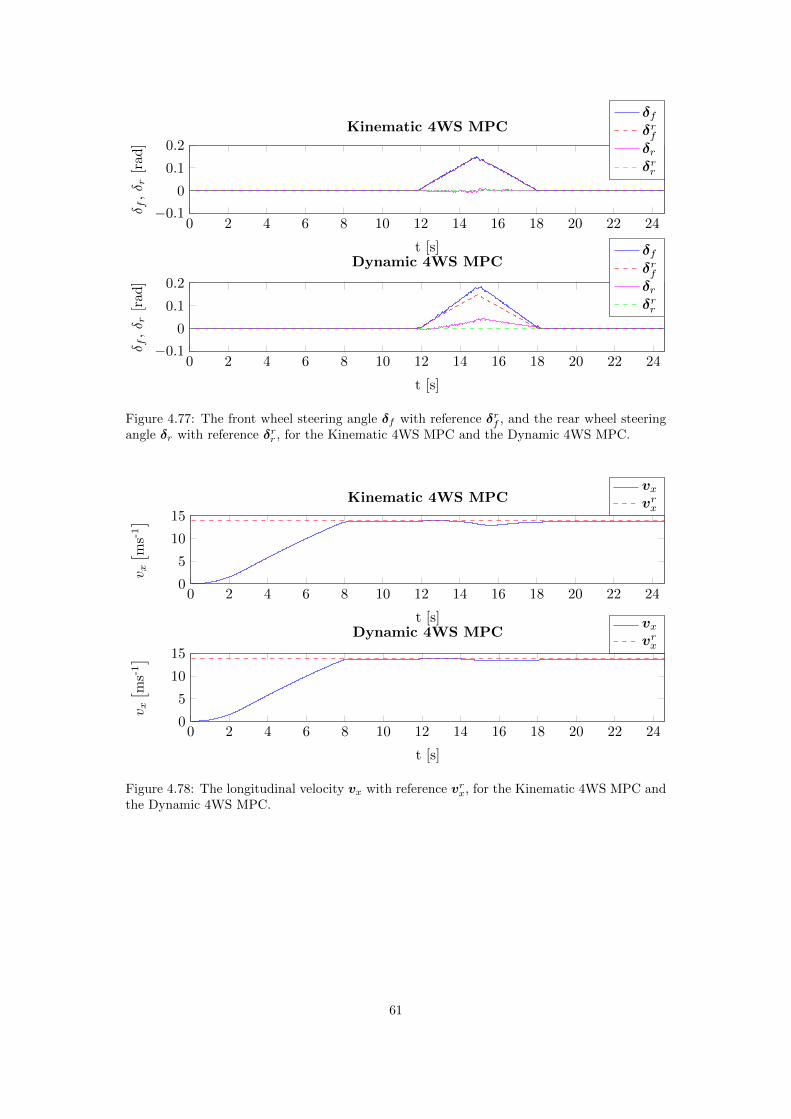
0 2 4 6 8 10 12 14 16 18 20 22 24−0.1
0
0.1
0.2
t [s]
δ f,δ r
[rad]
Kinematic 4WS MPCδfδrfδrδrr
0 2 4 6 8 10 12 14 16 18 20 22 24−0.1
0
0.1
0.2
t [s]
δ f,δ r
[rad]
Dynamic 4WS MPCδfδrfδrδrr
Figure 4.77: The front wheel steering angle δf with reference δrf , and the rear wheel steeringangle δr with reference δrr , for the Kinematic 4WS MPC and the Dynamic 4WS MPC.
0 2 4 6 8 10 12 14 16 18 20 22 240
5
10
15
t [s]
v x[ m
s-1]
Kinematic 4WS MPCvxvrx
0 2 4 6 8 10 12 14 16 18 20 22 240
5
10
15
t [s]
v x[ m
s-1]
Dynamic 4WS MPCvxvrx
Figure 4.78: The longitudinal velocity vx with reference vrx, for the Kinematic 4WS MPC andthe Dynamic 4WS MPC.
61
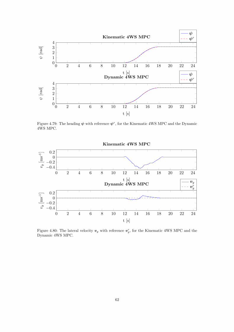
0 2 4 6 8 10 12 14 16 18 20 22 2401234
t [s]
ψ[rad
]Kinematic 4WS MPC
ψψr
0 2 4 6 8 10 12 14 16 18 20 22 2401234
t [s]
ψ[rad
]
Dynamic 4WS MPCψψr
Figure 4.79: The heading ψ with reference ψr, for the Kinematic 4WS MPC and the Dynamic4WS MPC.
0 2 4 6 8 10 12 14 16 18 20 22 24
−0.4−0.2
00.2
t [s]
v y[ m
s-1]
Kinematic 4WS MPC
0 2 4 6 8 10 12 14 16 18 20 22 24
−0.4−0.2
00.2
t [s]
v y[ m
s-1]
Dynamic 4WS MPCvyvry
Figure 4.80: The lateral velocity vy with reference vry, for the Kinematic 4WS MPC and theDynamic 4WS MPC.
62
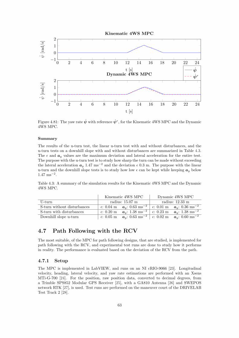
0 2 4 6 8 10 12 14 16 18 20 22 24−1
0
1
2
t [s]
ψ[rad/s]
Kinematic 4WS MPC
0 2 4 6 8 10 12 14 16 18 20 22 24−1
0
1
2
t [s]
ψ[rad/s]
Dynamic 4WS MPCψ
ψr
Figure 4.81: The yaw rate ψ with reference ψr, for the Kinematic 4WS MPC and the Dynamic4WS MPC.
Summary
The results of the u-turn test, the linear u-turn test with and without disturbances, and theu-turn tests on a downhill slope with and without disturbances are summarized in Table 4.3.The ε and ay values are the maximum deviation and lateral acceleration for the entire test.The purpose with the u-turn test is to study how sharp the turn can be made without exceedingthe lateral acceleration ay 1.47 ms−2 and the deviation ε 0.3 m. The purpose with the linearu-turn and the downhill slope tests is to study how low ε can be kept while keeping ay below1.47 ms−2.
Table 4.3: A summary of the simulation results for the Kinematic 4WS MPC and the Dynamic4WS MPC.
Kinematic 4WS MPC Dynamic 4WS MPCU-turn radius: 15.07 m radius: 12.33 mS-turn without disturbances ε: 0.04 m ay: 0.63 ms−2 ε: 0.01 m ay: 0.36 ms−2
S-turn with disturbances ε: 0.20 m ay: 1.38 ms−2 ε: 0.23 m ay: 1.38 ms−2
Downhill slope u-turn ε: 0.05 m ay: 0.63 ms−2 ε: 0.02 m ay: 0.60 ms−2
4.7 Path Following with the RCV
The most suitable, of the MPC for path following designs, that are studied, is implemented forpath following with the RCV, and experimental test runs are done to study how it performsin reality. The performance is evaluated based on the deviation of the RCV from the path.
4.7.1 Setup
The MPC is implemented in LabVIEW, and runs on an NI cRIO-9066 [23]. Longitudinalvelocity, heading, lateral velocity, and yaw rate estimations are performed with an XsensMTi-G-700 [24]. For the position, raw position data, converted to decimal degrees, froma Trimble SPS852 Modular GPS Receiver [25], with a GA810 Antenna [26] and SWEPOSnetwork RTK [27], is used. Test runs are performed on the maneuver court of the DRIVELABTest Track 2 [28].
63
4.7.2 Implementation
The MPC is implemented as explained in Section 4.1. The QP problem is solved using theQuadratic Programming VI in LabVIEW. The problem is solved with an active set algorithmand “warm start”, because of the shorter solver times compared to the interior point algorithmalso available with the Quadratic Programming VI.
The position and heading references are generated by first driving the intended path man-ually, recording the position and heading data. The samples from the recorded position data,that are to be used as the reference points, are chosen so that they are as uniformly spaced aspossible. Then the mean euclidean distance between them is set to be ∆(X,Y ). The samplesof the recorded heading data, that correspond to the chosen position references, are used asthe heading references. The heading references are also averaged by, for each reference point,making them the average of a certain number of reference points behind and ahead. Theremaining references are generated as described in Section 4.1.4, with the exception that thereferences for all of the states and control inputs, for the entire path, are generated offline toreduce computations when the controller is running. Practically, this means that all of thereferences are generated in the Path Generator, as seen in Figure 4.1.
The coordinates from the Trimble SPS852 Modular GPS Receiver are converted to lo-cal Cartesian coordinates. The conversion begins with converting the GPS coordinates fromgeodetic latitude and longitude to flat earth coordinates by finding the changes between theinitial longitude ι0 and the current longitude ι(k), and the initial latitude µ0 and the currentlatitude µ(k), resulting in
dι(k) = ι(k)− ι0, (4.12a)
dµ(k) = µ(k)− µ0. (4.12b)
The conversion uses the radius of curvature in the prime vertical RN and radius of curvaturein the meridian RM , defined as
RN =R√
1− (2f − f2) sin2(µ0), (4.13a)
RM = RN1− 2f − f2
1− (2f − f2) sin2(µ0), (4.13b)
[29], whereR = 6, 378, 137 m is the equatorial radius, or semi-major axis, and f = 1/298.257223563is the earth flattening [30]. Changes in the east, and north positions, dE(k) and dN(k), re-spectively, are approximated with
dE(k) =dι(k)
tan−1(
1RN cos(µ0)
) , (4.14a)
dN(k) =dµ(k)
tan−1(
1RM
) . (4.14b)
[29]. The flat earth coordinates are converted into meters with
X(k) =dE(k)π
180, (4.15a)
Y (k) =dN(k)π
180. (4.15b)
Due to the limited performance of the cRIO-9066, the most suitable, of the MPC designsstudied, is the Kinematic 2WS MPC. This is, because of the reduced complexity of it, com-pared to the others, the computations are reduced to be as simple as possible. The limited
64
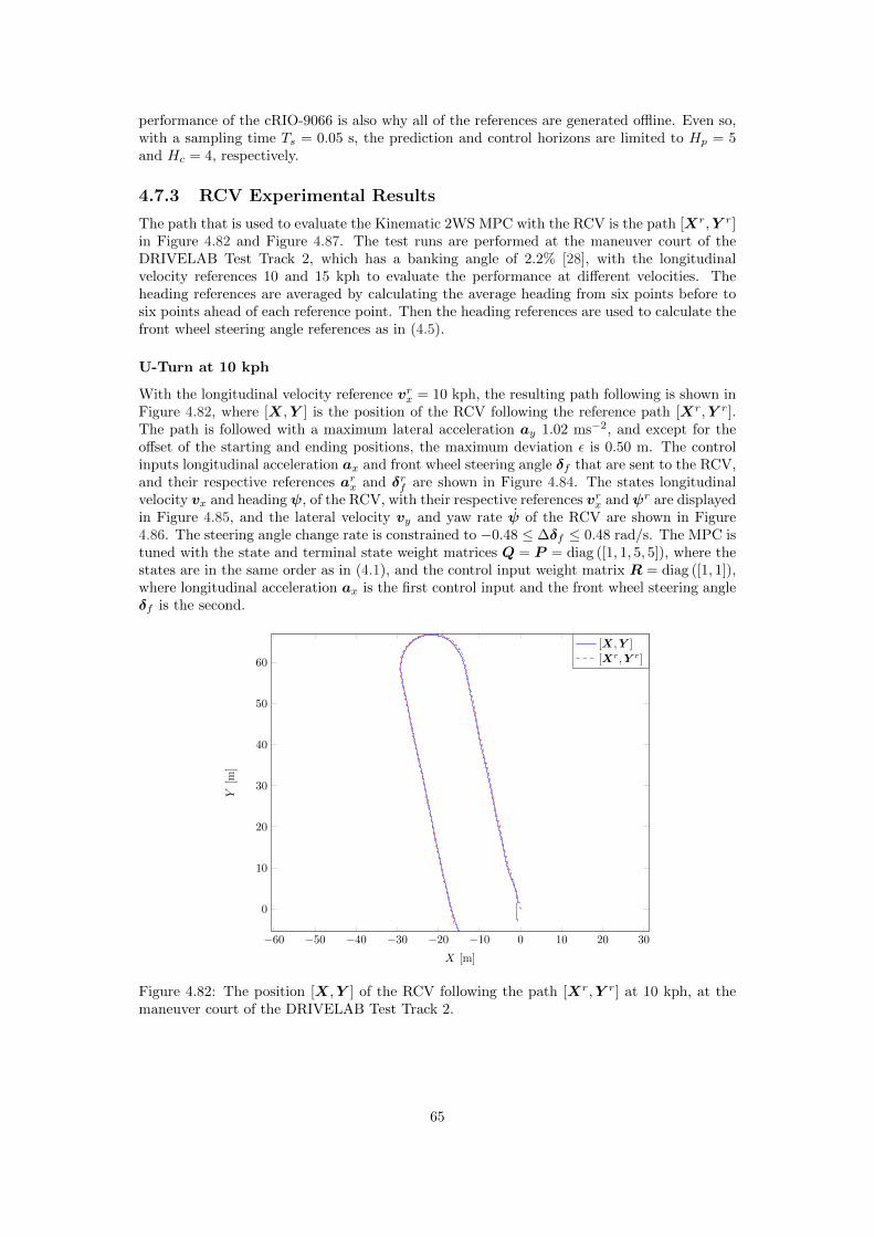
performance of the cRIO-9066 is also why all of the references are generated offline. Even so,with a sampling time Ts = 0.05 s, the prediction and control horizons are limited to Hp = 5and Hc = 4, respectively.
4.7.3 RCV Experimental Results
The path that is used to evaluate the Kinematic 2WS MPC with the RCV is the path [Xr,Y r]in Figure 4.82 and Figure 4.87. The test runs are performed at the maneuver court of theDRIVELAB Test Track 2, which has a banking angle of 2.2% [28], with the longitudinalvelocity references 10 and 15 kph to evaluate the performance at different velocities. Theheading references are averaged by calculating the average heading from six points before tosix points ahead of each reference point. Then the heading references are used to calculate thefront wheel steering angle references as in (4.5).
U-Turn at 10 kph
With the longitudinal velocity reference vrx = 10 kph, the resulting path following is shown inFigure 4.82, where [X,Y ] is the position of the RCV following the reference path [Xr,Y r].The path is followed with a maximum lateral acceleration ay 1.02 ms−2, and except for theoffset of the starting and ending positions, the maximum deviation ε is 0.50 m. The controlinputs longitudinal acceleration ax and front wheel steering angle δf that are sent to the RCV,and their respective references arx and δrf are shown in Figure 4.84. The states longitudinalvelocity vx and heading ψ, of the RCV, with their respective references vrx and ψr are displayedin Figure 4.85, and the lateral velocity vy and yaw rate ψ of the RCV are shown in Figure4.86. The steering angle change rate is constrained to −0.48 ≤ ∆δf ≤ 0.48 rad/s. The MPC istuned with the state and terminal state weight matrices Q = P = diag ([1, 1, 5, 5]), where thestates are in the same order as in (4.1), and the control input weight matrix R = diag ([1, 1]),where longitudinal acceleration ax is the first control input and the front wheel steering angleδf is the second.
−60 −50 −40 −30 −20 −10 0 10 20 30
0
10
20
30
40
50
60
X [m]
Y[m
]
[X,Y ]
[Xr,Y r]
Figure 4.82: The position [X,Y ] of the RCV following the path [Xr,Y r] at 10 kph, at themaneuver court of the DRIVELAB Test Track 2.
65
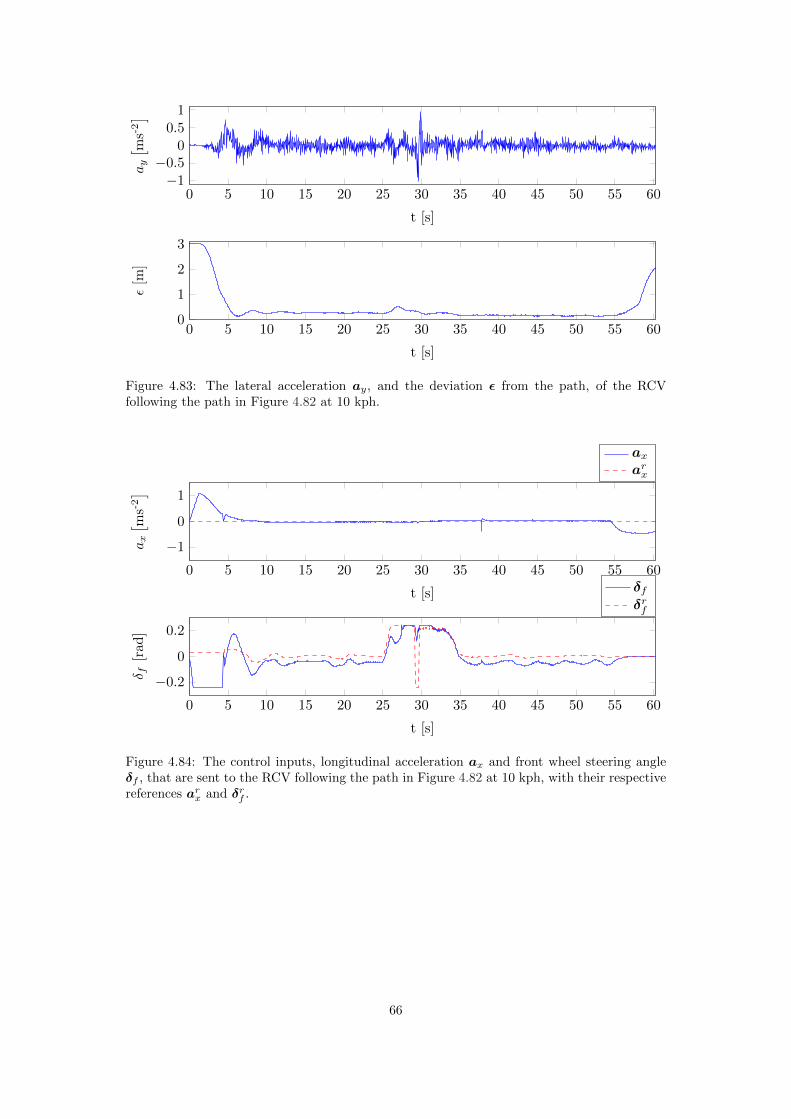
0 5 10 15 20 25 30 35 40 45 50 55 60−1
−0.50
0.51
t [s]
ay
[ ms-2]
0 5 10 15 20 25 30 35 40 45 50 55 600
1
2
3
t [s]
ε[m
]
Figure 4.83: The lateral acceleration ay, and the deviation ε from the path, of the RCVfollowing the path in Figure 4.82 at 10 kph.
0 5 10 15 20 25 30 35 40 45 50 55 60
−1
0
1
t [s]
ax
[ ms-2]
ax
arx
0 5 10 15 20 25 30 35 40 45 50 55 60
−0.2
0
0.2
t [s]
δ f[rad
]
δfδrf
Figure 4.84: The control inputs, longitudinal acceleration ax and front wheel steering angleδf , that are sent to the RCV following the path in Figure 4.82 at 10 kph, with their respectivereferences arx and δrf .
66
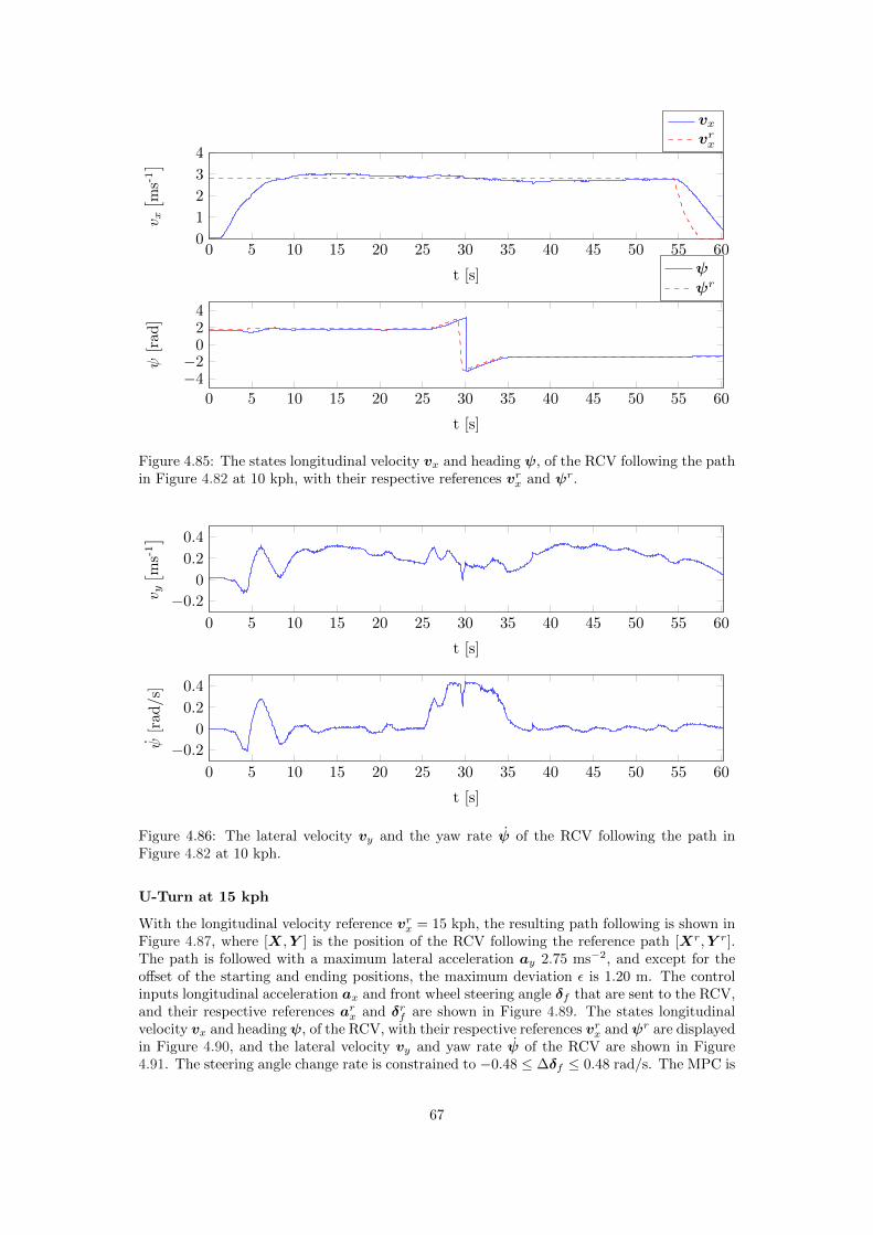
0 5 10 15 20 25 30 35 40 45 50 55 600
1
2
3
4
t [s]
v x[ m
s-1]
vxvrx
0 5 10 15 20 25 30 35 40 45 50 55 60
−4−2024
t [s]
ψ[rad]
ψψr
Figure 4.85: The states longitudinal velocity vx and heading ψ, of the RCV following the pathin Figure 4.82 at 10 kph, with their respective references vrx and ψr.
0 5 10 15 20 25 30 35 40 45 50 55 60
−0.2
0
0.2
0.4
t [s]
v y[ m
s-1]
0 5 10 15 20 25 30 35 40 45 50 55 60
−0.2
0
0.2
0.4
t [s]
ψ[rad
/s]
Figure 4.86: The lateral velocity vy and the yaw rate ψ of the RCV following the path inFigure 4.82 at 10 kph.
U-Turn at 15 kph
With the longitudinal velocity reference vrx = 15 kph, the resulting path following is shown inFigure 4.87, where [X,Y ] is the position of the RCV following the reference path [Xr,Y r].The path is followed with a maximum lateral acceleration ay 2.75 ms−2, and except for theoffset of the starting and ending positions, the maximum deviation ε is 1.20 m. The controlinputs longitudinal acceleration ax and front wheel steering angle δf that are sent to the RCV,and their respective references arx and δrf are shown in Figure 4.89. The states longitudinalvelocity vx and heading ψ, of the RCV, with their respective references vrx and ψr are displayedin Figure 4.90, and the lateral velocity vy and yaw rate ψ of the RCV are shown in Figure4.91. The steering angle change rate is constrained to −0.48 ≤ ∆δf ≤ 0.48 rad/s. The MPC is
67
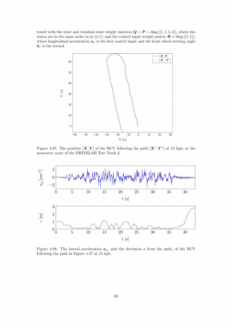
tuned with the state and terminal state weight matrices Q = P = diag ([1, 1, 5, 5]), where thestates are in the same order as in (4.1), and the control input weight matrix R = diag ([1, 1]),where longitudinal acceleration ax is the first control input and the front wheel steering angleδf is the second.
−60 −50 −40 −30 −20 −10 0 10 20 30
0
10
20
30
40
50
60
X [m]
Y[m
]
[X,Y ]
[Xr,Y r]
Figure 4.87: The position [X,Y ] of the RCV following the path [Xr,Y r] at 15 kph, at themaneuver court of the DRIVELAB Test Track 2.
0 5 10 15 20 25 30 35 40
−2
0
2
t [s]
ay
[ ms-2]
0 5 10 15 20 25 30 35 400
1
2
3
t [s]
ε[m
]
Figure 4.88: The lateral acceleration ay, and the deviation ε from the path, of the RCVfollowing the path in Figure 4.87 at 15 kph.
68
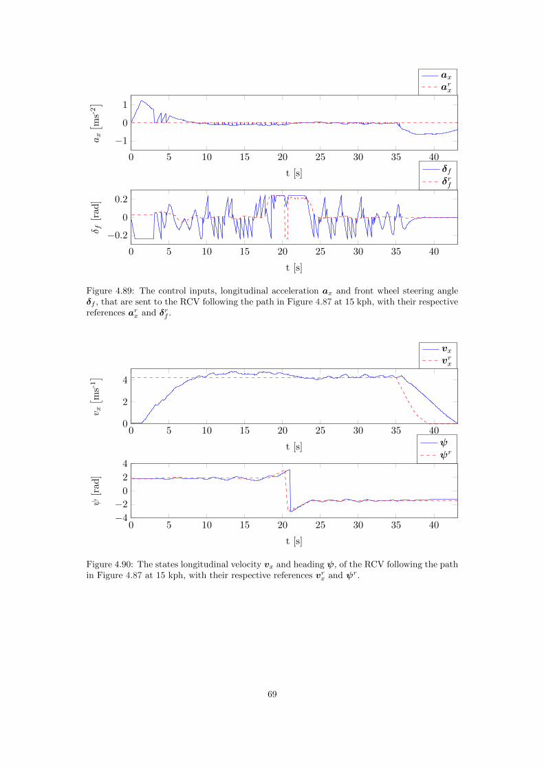
0 5 10 15 20 25 30 35 40
−1
0
1
t [s]
ax
[ ms-2]
ax
arx
0 5 10 15 20 25 30 35 40
−0.2
0
0.2
t [s]
δ f[rad
]
δfδrf
Figure 4.89: The control inputs, longitudinal acceleration ax and front wheel steering angleδf , that are sent to the RCV following the path in Figure 4.87 at 15 kph, with their respectivereferences arx and δrf .
0 5 10 15 20 25 30 35 400
2
4
t [s]
v x[ m
s-1]
vxvrx
0 5 10 15 20 25 30 35 40−4
−2
0
2
4
t [s]
ψ[rad
]
ψψr
Figure 4.90: The states longitudinal velocity vx and heading ψ, of the RCV following the pathin Figure 4.87 at 15 kph, with their respective references vrx and ψr.
69
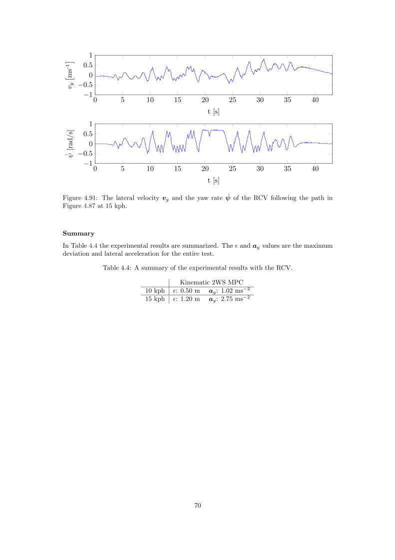
0 5 10 15 20 25 30 35 40−1
−0.5
0
0.5
1
t [s]
v y[ m
s-1]
0 5 10 15 20 25 30 35 40−1
−0.5
0
0.5
1
t [s]
ψ[rad
/s]
Figure 4.91: The lateral velocity vy and the yaw rate ψ of the RCV following the path inFigure 4.87 at 15 kph.
Summary
In Table 4.4 the experimental results are summarized. The ε and ay values are the maximumdeviation and lateral acceleration for the entire test.
Table 4.4: A summary of the experimental results with the RCV.
Kinematic 2WS MPC10 kph ε: 0.50 m ay: 1.02 ms−2
15 kph ε: 1.20 m ay: 2.75 ms−2
70
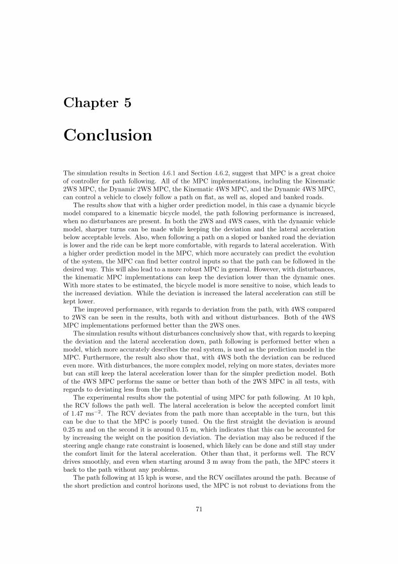
Chapter 5
Conclusion
The simulation results in Section 4.6.1 and Section 4.6.2, suggest that MPC is a great choiceof controller for path following. All of the MPC implementations, including the Kinematic2WS MPC, the Dynamic 2WS MPC, the Kinematic 4WS MPC, and the Dynamic 4WS MPC,can control a vehicle to closely follow a path on flat, as well as, sloped and banked roads.
The results show that with a higher order prediction model, in this case a dynamic bicyclemodel compared to a kinematic bicycle model, the path following performance is increased,when no disturbances are present. In both the 2WS and 4WS cases, with the dynamic vehiclemodel, sharper turns can be made while keeping the deviation and the lateral accelerationbelow acceptable levels. Also, when following a path on a sloped or banked road the deviationis lower and the ride can be kept more comfortable, with regards to lateral acceleration. Witha higher order prediction model in the MPC, which more accurately can predict the evolutionof the system, the MPC can find better control inputs so that the path can be followed in thedesired way. This will also lead to a more robust MPC in general. However, with disturbances,the kinematic MPC implementations can keep the deviation lower than the dynamic ones.With more states to be estimated, the bicycle model is more sensitive to noise, which leads tothe increased deviation. While the deviation is increased the lateral acceleration can still bekept lower.
The improved performance, with regards to deviation from the path, with 4WS comparedto 2WS can be seen in the results, both with and without disturbances. Both of the 4WSMPC implementations performed better than the 2WS ones.
The simulation results without disturbances conclusively show that, with regards to keepingthe deviation and the lateral acceleration down, path following is performed better when amodel, which more accurately describes the real system, is used as the prediction model in theMPC. Furthermore, the result also show that, with 4WS both the deviation can be reducedeven more. With disturbances, the more complex model, relying on more states, deviates morebut can still keep the lateral acceleration lower than for the simpler prediction model. Bothof the 4WS MPC performs the same or better than both of the 2WS MPC in all tests, withregards to deviating less from the path.
The experimental results show the potential of using MPC for path following. At 10 kph,the RCV follows the path well. The lateral acceleration is below the accepted comfort limitof 1.47 ms−2. The RCV deviates from the path more than acceptable in the turn, but thiscan be due to that the MPC is poorly tuned. On the first straight the deviation is around0.25 m and on the second it is around 0.15 m, which indicates that this can be accounted forby increasing the weight on the position deviation. The deviation may also be reduced if thesteering angle change rate constraint is loosened, which likely can be done and still stay underthe comfort limit for the lateral acceleration. Other than that, it performs well. The RCVdrives smoothly, and even when starting around 3 m away from the path, the MPC steers itback to the path without any problems.
The path following at 15 kph is worse, and the RCV oscillates around the path. Because ofthe short prediction and control horizons used, the MPC is not robust to deviations from the
71
references, which can be caused by fluctuating sensor measurements. At low velocities the MPCcan compensate for small deviations, but at higher velocities the MPC cannot appropriatelycompensate. The MPC overcompensates for the deviations, which can lead to oscillations orin the worst case, the MPC can become unstable. By increasing the horizons of the MPC itbecomes more robust to deviations, which ultimately leads to better path following. This canfor example be done by increasing the sampling time, and with a longer sampling period theprediction and control horizons can potentially be increased which would further increase thehorizon. Except for increasing the horizons, the MPC can be made more robust to positiondeviations by increasing the weight on the heading. This can reduce the oscillations, but canalso lead the deviation from the path to be too large because the MPC does not minimize thedeviation from the path as much. Another way can be to loosen the constraints on the steeringchange rate so that the MPC may find a better control input and not overcompensate. Inthis case, it is not a good solution if the ride comfort is to be maintained, because the lateralacceleration is already above the maximum comfort limit.
One more thing that can have a negative impact on the performance of the path followingis poor reference generation. Generating the path as described in Section 4.7.2 means mea-surement errors and noise affect the quality of the references. The noise and errors from theheading references are amplified when calculating the references for the front wheel steeringangle. Even when averaging the heading references, over thirteen points, to reduce the noise,it is still evident in the front wheel steering angle references.
The results also show that with the Kinematic 2WS MPC, and especially with the shortprediction and control horizons used, only low velocities can be handled. With longer predic-tion and control horizons, the MPC will also be able to handle higher velocities, as shown bythe simulation results.
Comparing the experimental results with the simulation results, the impact of havingshorter prediction and control horizons and the impact of measurement noise becomes clear.This suggests that if the prediction and control horizons can be increased and if measurementnoise is reduced, the performance of the MPC for path following can be very good.
5.1 Future Work
A reliable way of generating accurate position references for the MPC is needed. This couldfor example be by generating paths from map services. To further improve the path following,more sophisticated path planning is also needed. This is especially important in a dynamicenvironment, for example in the case of avoiding moving or static obstacles. The path planneris needed to be able to determine if and how obstacles can be avoided in a safe manner. Thepath planner will supply the controller with appropriate references, for example, new positionreferences if the path is changed, to lower the speed or stop altogether if needed. When it isrequired to drive at different velocities and handle turns with different curvatures, the needfor path planning is also increased. The path planner must provide velocity references tothe controller, so that the speed can be lowered if needed and the turn made at a safe andcomfortable speed.
If the path planner is good enough, it may not be needed to use an MPC for the longitudinalcontrol of a vehicle. In this case a simpler, such as a PID controller can be used instead. Thiswill reduce the complexity of the MPC, leading to faster solver times. With faster solver times,the prediction and control horizons can be increased, leading to a more robust controller.
In the case of running the MPC on the cRIO-9066, it can be an improvement to only dolateral control with the MPC. The performance of the cRIO-9066 only allows for short horizonsor long sampling periods when doing both longitudinal and lateral control. Reducing the MPCto only perform lateral control, reduces the complexity of the MPC, which leads to shortersolver times. The reduced solver times leads to several ways of improving the path followingperformance of the MPC, when performing path following with the RCV. It is important tomake the MPC more robust to sensor noise and reference deviations. One way is to increasethe prediction and control horizons, and another is to use a more accurate system model as the
72
prediction model in the MPC, for example a dynamic bicycle model. The drawback of usingthe dynamic bicycle model, is that, in addition to estimating the states velocity, heading, andposition, as with a kinematic model, lateral speed and yaw rate will also have to be estimated.This means that a poorly functioning state estimation can have a negative impact on the pathfollowing.
Except for making the MPC more robust, a way of improving the path following perfor-mance, when sensor noise is present, is to improve the state estimation. Noise in the headingand position measurements, is particularly important to reduce when it is essential to keepthe deviation from the path down. The position data from the Trimble SPS852, with net-work RTK, is accurate, but by implementing sensor fusion with an IMU, the accuracy canpotentially be improved. Also, the heading estimation from the Xsens MTi-G-700 is accuratewhen the RCV is moving, but soon after it stops, the heading angle starts to drift. With twoaccurate GPS receivers, both of them can be used to improve the heading estimation especiallywhen standing still.
Another improvement which can be made is to implement 4WS MPC with the RCV,so that the front and rear wheels can be controlled independently from each other. Thesimulation results suggests that there are advantages with controlling the front and rear wheelsindependently from each other, when it comes to reducing lateral acceleration and deviationfrom the path.
73
Bibliography
[1] P. Falcone, F. Borrelli, J. Asgari, H. E. Tseng, and D. Hrovat, “A model predictivecontrol approach for combined braking and steering in autonomous vehicles,” in Control& Automation, 2007. MED’07. Mediterranean Conference on. IEEE, 2007, pp. 1–6.
[2] V. Milanes, D. F. Llorca, B. M. Vinagre, C. Gonzalez, and M. A. Sotelo, “Clavileno:Evolution of an autonomous car,” in Intelligent Transportation Systems (ITSC), 201013th International IEEE Conference on. IEEE, 2010, pp. 1129–1134.
[3] P. Falcone, F. Borrelli, H. Tsengz, J. Asgari, and D. Hrovat, “A hierarchical model predic-tive control framework for autonomous ground vehicles,” in American Control Conference,2008. IEEE, 2008, pp. 3719–3724.
[4] A. Sidhu, D. R. Mikesell, D. A. Guenther, R. Bixel, and G. J. Heydinger, “Develop-ment and implementation of a path-following algorithm for an autonomous vehicle,” SAETechnical paper, Tech. Rep., 2007.
[5] V. Turri, A. Carvalho, H. Tseng, K. H. Johansson, and F. Borrelli, “Linear model pre-dictive control for lane keeping and obstacle avoidance on low curvature roads,” in 201316th International IEEE Conference on Intelligent Transportation Systems: IntelligentTransportation Systems for All Modes, ITSC 2013; The Hague; Netherlands; 6 October2013 through 9 October 2013. IEEE, 2013, pp. 378–383.
[6] R. Rajamani, Vehicle dynamics and control. Springer Science & Business Media, 2011.
[7] P. Tomner, “Design and implementation of control and actuation for an over-actuatedresearch vehicle,” Master’s thesis, KTH Royal Institute of Technology, 2014.
[8] KTH Smart Mobility Lab. KTH Research Concept Vehicle. Accessed: 2015-02-11.[Online]. Available: http://www.kth.se/ees/forskning/strategiska-forskningsomraden/intelligenta-transportsystem/smart-mobility-lab/projects/research-platforms-1.439400
[9] F. Borrelli, P. Falcone, T. Keviczky, and J. Asgari, “Mpc-based approach to active steeringfor autonomous vehicle systems,” International Journal of Vehicle Autonomous Systems,vol. 3, no. 2, pp. 265–291, 2005.
[10] T. Besselmann and M. Morari, “Hybrid parameter-varying model predictive control forautonomous vehicle steering,” European Journal of Control, vol. 14, no. 5, pp. 418–431,2008.
[11] P. Falcone, H. Eric Tseng, F. Borrelli, J. Asgari, and D. Hrovat, “Mpc-basedyaw and lateral stabilisation via active front steering and braking,” VehicleSystem Dynamics, vol. 46, no. sup1, pp. 611–628, 2008. [Online]. Available:http://dx.doi.org/10.1080/00423110802018297
[12] Y. Yoon, J. Shin, H. J. Kim, Y. Park, and S. Sastry, “Model-predictiveactive steering and obstacle avoidance for autonomous ground vehicles,” ControlEngineering Practice, vol. 17, no. 7, pp. 741 – 750, 2009. [Online]. Available:http://www.sciencedirect.com/science/article/pii/S0967066108002025
74
[13] D. Q. Mayne, J. B. Rawlings, C. V. Rao, and P. O. Scokaert, “Constrained model pre-dictive control: Stability and optimality,” Automatica, vol. 36, no. 6, pp. 789–814, 2000.
[14] F. Kuhne, W. F. Lages, and J. GOMES da SILVA, “Mobile robot trajectory trackingusing model predictive control,” in II IEEE latin-american robotics symposium, 2005.
[15] P. Falcone, F. Borrelli, J. Asgari, H. Tseng, and D. Hrovat, “Predictive active steeringcontrol for autonomous vehicle systems,” Control Systems Technology, IEEE Transactionson, vol. 15, no. 3, pp. 566–580, May 2007.
[16] F. Borrelli, P. Falcone, T. Keviczky, and J. Asgari, “Mpc-based approach to active steeringfor autonomous vehicle systems,” International Journal of Vehicle Autonomous Systems,vol. 3, no. 2, pp. 265–291, 2005.
[17] D. Limon, I. Alvarado, T. Alamo, and E. F. Camacho, “Mpc for tracking piecewiseconstant references for constrained linear systems,” Automatica, vol. 44, no. 9, pp. 2382–2387, 2008.
[18] M. Kvasnica, Real-time model predictive control via multi-parametric programming: theoryand tools. VDM-Verlag, 2009.
[19] L. Zhang and X. Zhuan, “Optimal operation of heavy-haul trains equipped with electron-ically controlled pneumatic brake systems using model predictive control methodology,”Control Systems Technology, IEEE Transactions on, vol. 22, no. 1, pp. 13–22, 2014.
[20] E. Wennerstrom, S. Nordmark, and B. Thorvald, “Vehicle dynamics,” KTH Vehicle Dy-namics, Aeronautical and Vehicle Engineering, KTH Royal Institute of Technology, 2011.
[21] J. Mattingley and S. Boyd. (2015-06-11) CVXGEN. [Online]. Available: http://cvxgen.com/docs/index.html
[22] A. Kilinc and T. Baybura, “Determination of minimum horizontal curve radius used inthe design of transportation structures, depending on the limit value of comfort criterionlateral jerk,” 2012.
[23] National Instruments. (2015-06-10) NI cRIO-9066. [Online]. Available: http://sine.ni.com/nips/cds/view/p/lang/sv/nid/212805
[24] Xsens. (2015-08-03) MTi-G-700. [Online]. Available: https://www.xsens.com/products/mti-g-700/
[25] Trimble. (2015-08-11) Trimble SPS852 Modular GPS Receiver. [Online]. Available:http://trl.trimble.com/docushare/dsweb/Get/Document-490932
[26] Trimble. (2015-08-11) GA810 Antenna. [Online]. Available: http://intech.trimble.com/oem gnss/antennas/ga810
[27] SWEPOS. (2015-08-11) SWEPOS Natverks-RTK-tjanst. [Online]. Available: https://swepos.lantmateriet.se/tjanster/realtid/natverksrtk/natverksrtk.aspx
[28] DRIVELAB. (2015-06-10) Test Track 2. [Online]. Available: http://drivelab.se/test-track-2/
[29] MathWorks. (2015-08-17) lla2flat. [Online]. Available: http://se.mathworks.com/help/aerotbx/ug/lla2flat.html
[30] National Imagery and Mapping Agency, “Department of Defense World Geodetic Sys-tem 1984 Its Definition and Relationships with Local Geodetic Systems,” NATIONALIMAGERY AND MAPPING AGENCY TECHNICAL REPORT 8350.2, vol. 3, 2000.
75

TRITA EE 2015-77
ISSN 1653-5146
www.kth.se