Impact of Electric Vehicle Charging on The Power Grid

Subtitle

Shimi Sudha Letha Math Bollen

Impact of Electric Vehicle Charging on The Power Grid

Subtitle

Shimi Sudha LethaMath Bollen

Luleå University of TechnologyDepartment of Engineering Sciences and Mathematics

Division of Energy Science

ISSN 1402-1536

ISBN 978-91-7790-763-3 (pdf)

Luleå 2021

www.ltu.se

IMPACT OF ELECTRIC VEHICLE CHARGING ON

THE POWER GRID

SHIMI SUDHA LETHA MATH BOLLEN

January 2021

2

PREFACE

This report has been written as part of a project supported by the Swedish Energy Agency

(“Energimyndigheten”). The project is entitled “Interaction between charging infrastructure

with electromobility and the electricity grid” and it is conducted by the Electric Power

Engineering Group at Luleå University of Technology in Skellefteå, Sweden.

In the first phase of this project a pilot study was carried out for a period of 10 months. At the

completion of the first phase the challenges regarding EV charging were published as a report and

disseminated in a workshop. At the second phase of this project advance studies were carried out

and the report summarizes the synthesis of knowledge, research results and challenges regarding

connection of large amounts of Electric vehicles to the electricity grid.

This report summarizes the results of different studies carried out by the members of the

Electric Power Engineering group. The discussions were led by Math Bollen and Shimi Sudha

Letha. Different persons who have contributed to the different sections in this report are,

1. Introduction: Shimi Sudha Letha and Math Bollen

2. Waveform Distortion due to EV charging (propagation and aggregation): Naser Nakhodchi,

Vineetha Ravindran, Selçuk Sakar

3. Voltage dips, fault-ride-through: Roger Alves de Oliveira

4. Fast voltage fluctuations and light flicker: Elena Gutiérrez Ballesteros, Selçuk Sakar and

Shimi Sudha Letha

5. Undervoltages and PV-EV hosting capacity: Enock Mulenga

6. Overloading, dynamic rating of component : Fatemeh Hajeforosh

7. Overloading and reliability of grid : Hamed Bakhtiari and Kazi Main Uddin Ahmed

8. Impact of EV charging on neutral and protective earth: Jil Sutaria

9. Larger installation for EV charging technology and its impact on reliability: Zunaira Nazir

10. Impact of temperature on EV charging : Shimi Sudha Letha

11. Conclusion: Shimi Sudha Letha and Math Bollen with input from all project members

3

SUMMARY

This report summarizes the situation with knowledge and challenges regarding the large-scale

introduction of electromobility in the Swedish power grid.

The content covers a range of systemic perspectives in terms of challenges and impacts that

the fast-growing amount of charging associated with electromobility poses to the actual power

system. From this, several important questions are addressed in order to predict the future positive

and negative impacts of this.

The focus is placed on the possible impacts on the low and medium voltage networks, mainly

exploring the power quality issues and grid hosting capacity. The following power quality issues

are addressed: RMS voltage (slow voltage variation, overvoltage, undervoltage, fast voltage

variations), unbalance, waveform distortion (harmonics, interharmonics, and supraharmonics),

and power system stability. The hosting capacity is examined to predict whether the charging

demand from electromobility can be accommodated in the existing power system considering the

involved challenges.

Furthermore, the aspect related to the charging process and people’s traveling patterns under a

stochastic point of view is analysed. With the advantages that electromobility brings, it is

noticeable that people will change the way they move around. Insights from this perspective make

it possible to predict how the grid needs to change to accommodate future needs.

From the found evidence in this report, it is noticed that the harmonic content of the current

injected from electric vehicles charging is not negligible, though its magnitude is low it may get

aggregated with harmonics produced by other connected loads in the low voltage network.

Additionally, the results from leakage current (due to supraharmonics) in protective earth, light

flicker and voltage dip studies show potential issue due to the charging process. Further, this study

determines the hosting capacity of EVs based on the PV – EV integration, dynamic line rating,

curtailment (hr/yr) of large rated electric vehicles and temperature. The hosting capacity studies

estimated a significant surplus capacity for EV penetration under the present grid condition in

Sweden. But considering certain level of risk especially during winters proper planning is required.

Other evidences from this report provides additional support for future discussions and debates

regarding the impacts of electromobility on the electrical system.

4

CONTENTS

Preface 2

Summary 3

1. Introduction 5

2. Waveform Distortion due to EV Charging 6

2.1 Probability Density Function (PDF) of Dominant Harmonics 6

2.2 Interharmonics Aggregation in Time Domine 8

2.3 Supraharmonics in EVs 10

3. Impact of Voltage Dips in Electrical Vehicle Charging Stations 12

4. Impact of EV Charging Fast Voltage Fluctuations on Light Flicker 15

5. Impact of EV Charging on Neutral and Protective Earth 17

6. PV – EV Hosting Capacity Assesment in View of Undervoltage 21

7. Enhancement of Grid Capacity for EV Charging using Dynamic Line Rating 26

8. Distribution Transformer Overloading due to EV Integration and reliability:

A Stochastic Approach 28

9. Curtailment Demand Estimation Under Large EV Charging Load 33

10. Impact of Temperature on EV Hosting Capacity 35

11. Conclusion 38

12. References 40

5

1. INTRODUCTION

The new era of clean and efficient transport with advances in technology poses new social

and technical challenges to the modern electric grid. Most implementations of electromobility

envision large amount of electric vehicles (EVs) charging stations and electrification of roads fed

from the low or medium-voltage distribution network. Increasing load from the charging

infrastructure can set limits to the electricity grid and negatively impact other customers connected

to the grid.

There is limited knowledge and experience about the interaction and compatibility between

the charging infrastructure and the grid. There has been some research and studies on how large-

scale charging of electric cars affects the grid, especially in terms of overloading the grid and

voltage reductions. There is a limited amount of research on how much disturbances the grid can

handle (hosting capacity), but there is a lot of research on how coordinated charging of electric

cars (smart charging) can reduce the impact on the grid. Though there are publications on the

emission due to EV charging in literature, the fast growing technological innovation leads to

completely different emission pattern, introducing new challenges to the network operators and

the research community.

The major challenge here is to get suitable models about charging as a function of time. For

harmonics, the calculations are more complicated because it is necessary to include propagation

and aggregation effects along with the effect of nearby devices on each other's emission (primary

and secondary emissions). It is also uncertain what the emission will be from future charging

infrastructure. There are a lot of additional challenges here, as there are similarities with challenges

when connecting other types of new equipment to the electricity grid.

There are several similarities in terms of the impact on the electric network between charging

infrastructure and photovoltaic systems. With regard to the latter, a number of studies have been

carried out on how much the electric grids in Sweden can handle, however more research is

required to determine the hosting capacity of EVs considering the renewable energy generation,

ambient temperature, large charging installations, dynamic line rating etc.

The consequences of large-scale transition to electromobility will also lead to lack of

production capacity and congestion of the transmission network during certain high-load hours.

The solution to this is the participation of the EVs in the electricity market. One consequence of

this, however, is that there will be a greater synchronization of the EVs with potential negative

consequences for distribution networks. There is very limited knowledge about these

consequences.

The report summarizes the synthesis of knowledge, research results and challenges regarding

connection of large amounts of electric vehicles to the low and medium voltage netwrok. The

project has mainly addressed the following challenges:

Propogation and aggregation of harmonics, interharmonics and supraharmonics in the

distribution network with charging infrastructure.

Fault ride through of charging infrastructure against voltage dips.

Impact of fast voltage fluctuations due to EV charging on light flicker.

Impact of EV charging on neutral and protective earth and tripping of RCD.

Acceptance limit for the combination of EV charging and solar power in distribution

networks.

Overloading due to EV charging when using dynamic rating of components.

Reliability and Curtailment estimation in the supply to cities with EV charging load.

Electric vehicle hosting capacity of a distribution network including ambient temperature.

6

2. WAVEFORM DISTORTION DUE TO EV CHARGING

The level of current harmonic emission from EV charging depends on charger circuit topology,

power level, on the supply voltage distortion (background distortion), and on the network

impedance. The simplest diode rectifiers emit high level of current harmonics but with

improvement in their circuits and control techniques, new chargers have much less harmonic

emission [1]. A complete charging cycle can be divided into two stages; constant current (CC) and

constant voltage (CV). The CC is the main charging period and starts from zero to almost 80%

SOC followed by CV until full charge. EV chargers behave differently in each stage from harmonic

point of view. During CC they have low harmonic distortion but during CV the current waveform

is more distorted [2]. Recently published work reports significant variation in THDi and individual

harmonics current among 18 different EVs on-board chargers [3].

The cancellation effect because of diversity of EVs and SOC of the batteries play significant

role in aggregation of slow chargers. Fast chargers (usually more than 40 kW) have fixed location

in the network compare with slow chargers, hence it is easier to manage and control them. Most

of charging stations utilize the same brand and model of EV chargers but still the diversity of EVs

and SOC of the batteries can add some level of uncertainty to the harmonic studies regarding fast

chargers.

EV harmonic studies can also be categorized to deterministic studies and stochastic studies.

Modelling the charger in time domain and frequency domain, investigating cancellation effect and

impact of background voltage on harmonic emission and estimation of EV hosting capacity in

terms of harmonic are the most discussed topic in deterministic studies. In stochastic approaches,

in order to have more realistic results, different types of uncertainty such as diversity of EVs,

diversity of SOCs, background voltage variation, location of the charger in the network, etc. , add

to the model.

2.1 Probability density function (PDF) of dominant harmonics

A stochastic harmonic study of a 375 A, 160 kW EV fast charger located in a winter car testing

centre in north Sweden is discussed. The extracted probability density functions (PDF) for

individual harmonic orders can be utilized as an input for any other stochastic model and Monte

Carlo simulation-based study in this field. Beside the continuous measurement of electrical

parameter (aggregation of 2 min interval), current and voltage waveform snapshots (200 ms with

12.8 kHz sampling frequency) were saved every 2 minutes for a period of one month. During

measurement period variety of EVs (anonymously) with different SOC were charged by this

charger, like the real situation. 96 charging cycles are considered for analysis with different total

charging powers, ranges from 25 kW to 150 kW and different charging period, ranges from 6 to

200 minutes. The boxplot of harmonic current for all harmonic orders until 40 is shown in Fig. 2.1

considering all values for these 96 charging cycles. As it is expected for a three-phase rectifier,

harmonic orders 5, 7, 11, 13 , 17 , 19 , 23, 25 have higher values, but interesting observation is for

even harmonics where 4th and 10th showed high emission. It can be because of the impact of dc

current on transformer saturation. Any asymmetry of gating driving pulses of semiconductor

switches can cause dc current and aggregation of these dc currents from different chargers in a

charging station can shift the transformer core to the saturation points and consequently causing

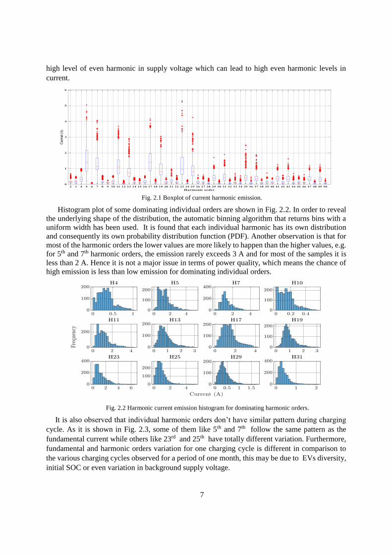
7

high level of even harmonic in supply voltage which can lead to high even harmonic levels in

current.

Fig. 2.1 Boxplot of current harmonic emission.

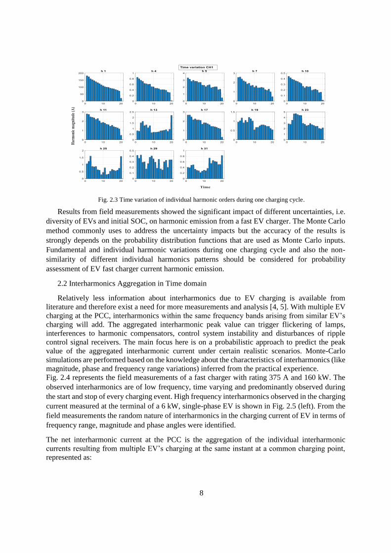
Histogram plot of some dominating individual orders are shown in Fig. 2.2. In order to reveal

the underlying shape of the distribution, the automatic binning algorithm that returns bins with a

uniform width has been used. It is found that each individual harmonic has its own distribution

and consequently its own probability distribution function (PDF). Another observation is that for

most of the harmonic orders the lower values are more likely to happen than the higher values, e.g.

for 5th and 7th harmonic orders, the emission rarely exceeds 3 A and for most of the samples it is

less than 2 A. Hence it is not a major issue in terms of power quality, which means the chance of

high emission is less than low emission for dominating individual orders.

Fig. 2.2 Harmonic current emission histogram for dominating harmonic orders.

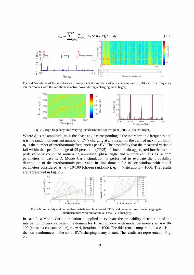
It is also observed that individual harmonic orders don’t have similar pattern during charging

cycle. As it is shown in Fig. 2.3, some of them like 5th and 7th follow the same pattern as the

fundamental current while others like 23rd and 25th have totally different variation. Furthermore,

fundamental and harmonic orders variation for one charging cycle is different in comparison to

the various charging cycles observed for a period of one month, this may be due to EVs diversity,

initial SOC or even variation in background supply voltage.

8

Fig. 2.3 Time variation of individual harmonic orders during one charging cycle.

Results from field measurements showed the significant impact of different uncertainties, i.e.

diversity of EVs and initial SOC, on harmonic emission from a fast EV charger. The Monte Carlo

method commonly uses to address the uncertainty impacts but the accuracy of the results is

strongly depends on the probability distribution functions that are used as Monte Carlo inputs.

Fundamental and individual harmonic variations during one charging cycle and also the non-

similarity of different individual harmonics patterns should be considered for probability

assessment of EV fast charger current harmonic emission.

2.2 Interharmonics Aggregation in Time domain

Relatively less information about interharmonics due to EV charging is available from

literature and therefore exist a need for more measurements and analysis [4, 5]. With multiple EV

charging at the PCC, interharmonics within the same frequency bands arising from similar EV’s

charging will add. The aggregated interharmonic peak value can trigger flickering of lamps,

interferences to harmonic compensators, control system instability and disturbances of ripple

control signal receivers. The main focus here is on a probabilistic approach to predict the peak

value of the aggregated interharmonic current under certain realistic scenarios. Monte-Carlo

simulations are performed based on the knowledge about the characteristics of interharmonics (like

magnitude, phase and frequency range variations) inferred from the practical experience.

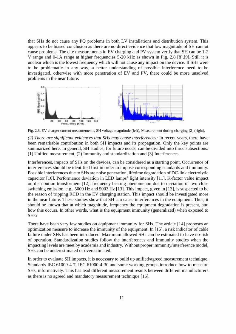
Fig. 2.4 represents the field measurements of a fast charger with rating 375 A and 160 kW. The

observed interharmonics are of low frequency, time varying and predominantly observed during

the start and stop of every charging event. High frequency interharmonics observed in the charging

current measured at the terminal of a 6 kW, single-phase EV is shown in Fig. 2.5 (left). From the

field measurements the random nature of interharmonics in the charging current of EV in terms of

frequency range, magnitude and phase angles were identified.

The net interharmonic current at the PCC is the aggregation of the individual interharmonic

currents resulting from multiple EV’s charging at the same instant at a common charging point,

represented as:

9

𝐼𝑖ℎ = ∑ ∑ 𝑛𝑓

𝑙=0 𝐴𝑙

𝑛

𝑘=0cos(2 𝜋𝑓𝑙𝑡 + ∅𝑙) (2.1)

Fig. 2.4 Variations of 0.5 interharmonic component during the start of a charging event (left) and low frequency

interharmonics with the variations in active power during a charging event (right).

Fig. 2.5 High frequency time-varying interharmonics spectrogram (left), 2D spectra (right).

Where 𝐴𝑙 is the amplitude, ∅𝑙 is the phase angle corresponding to the interharmonic frequency and

𝑛 is the random or constant number of EV’s charging at any instant in the defined maximum limit,

𝑛𝑓 is the number of interharmonic frequencies per EV. The probability that the measured variable

fall within the specified range of 95 percentile (CP95) of time domain aggregated interharmonic

peak value is computed initializing amplitude, phase angle and number of EV’s as random

parameters in case 1. A Monte Carlo simulation is performed to evaluate the probability

distribution of the interharmonic peak value in time domain for 10 sec window with model

parameters considered as: 𝑛 = 10-100 (chosen randomly), 𝑛𝑓 = 4, iterations = 1000. The results

are represented in Fig. 2.6.

Fig. 2.6 Probability and cumulative distribution function of CP95 peak value of time domain aggregated

interharmonics with randomness in the EV’s charging.

In case 2, a Monte Carlo simulation is applied to evaluate the probability distribution of the

interharmonic peak value in time domain for 10 sec window with model parameters as: 𝑛 = 10-

100 (chosen a constant value), 𝑛𝑓 = 4, iterations = 1000. The difference compared to case 1 is in

the non- randomness in the no: of EV’s charging at any instant. The results are represented in Fig.

2.7.

10

Fig. 2.7 Probability and cumulative distribution function of CP95 peak value of time domain aggregated

interharmonics with constant no: of EV’s charging.

Analysis of the data has shown that the time domain aggregation of interharmonic current from

multiple sources at PCC has a Type I extreme value distribution with PDF, defined as:

𝑓(𝑥) =1

𝜎 𝑒−

𝑥−𝜇

𝜎 𝑒−𝑒−

𝑥−𝜇𝜎 (2.2)

Where μ is the location parameter and 𝜎 is the scale parameter and zero shape parameter. It was

identified that both these parameters increases with the increase in the number of connected

devices whereas the 95 percentile probability of the peak value of interharmonic decreased almost

linearly with the increase in the number of connected devices. It was verified that the left skewness

was as a result of the randomness in the no. of connected EV’s. Whereas if the number of connected

EV’s was considered constant in second case, the left skewed extreme value distribution converged

to normal distribution. μ increases with the increase in the number of connected devices whereas

𝜎 and 95 percentile probability of the peak value of interharmonic remains almost constant

independent of the number of connected devices. Empirical relationships between μ and the

number of interharmonic frequencies at PCC from randomly connected devices in operation can

be approximated for both the cases [6].

It is inference that the prediction of aggregated interharmonic peak current with highest 95

percentile probability is possible if known the individual interharmonic spectra of the EV and thus

knowing the probable number of interharmonic frequencies aggregating at PCC. It was established

that the randomness in the number of frequency components that appear at the PCC due to the

randomness in the number of connected EVs (that interharmonic sources) is that matters for the

aggregated interharmonic peak value. This is visible from the skewness caused by the randomness

in the extreme value distribution and loss of skewness with constant number of EV’s. It was also

identified as part of this work that as the interharmonic frequencies which gets aggregated are of

higher frequencies and if the number of interharmonic sources and thus number of interharmonic

frequencies are less, the probability of getting a linear addition for peak value is more in shorter

time period [6].

2.3 Supraharmonics in EVs

Due to power electronics converter switching, EV charger emits high frequency emission,

specifically between 2-150 kHz named “Supraharmonics.” Supraharmonics (SHs) are under

discussion from many perspectives whether they are problematic or not. The main two opinions

are:

(1) SH measurement at EV charger: It is stated that front-end filters, each switching device has,

can sink SHs and limits its propagation into the grid [7]. Considering this fact, it was concluded

11

that SHs do not cause any PQ problems in both LV installations and distribution system. This

appears to be biased conclusion as there are no direct evidence that low magnitude of SH cannot

cause problems. The cite measurements in EV charging and PV system verify that SH can be 1-2

V range and 0-1A range at higher frequencies 5-20 kHz as shown in Fig. 2.8 [8],[9]. Still it is

unclear which is the lowest frequency which will not cause any impact on the device. If SHs were

to be problematic in any way, a better understanding of possible interference need to be

investigated, otherwise with more penetration of EV and PV, there could be more unsolved

problems in the near future.

Fig. 2.8. EV charger current measurements, SH voltage magnitude (left), Measurement during charging [2] (right).

(2) There are significant evidences that SHs may cause interferences: In recent years, there have

been remarkable contribution in both SH impacts and its propagation. Only the key points are

summarized here. In general, SH studies, for future needs, can be divided into three subsections:

(1) Unified measurement, (2) Immunity and standardization and (3) Interferences.

Interferences, impacts of SHs on the devices, can be considered as a starting point. Occurrence of

interferences should be identified first in order to impose corresponding standards and immunity.

Possible interferences due to SHs are noise generation, lifetime degradation of DC-link electrolytic

capacitor [10], Performance deviation in LED lamps’ light intensity [11], K-factor value impact

on distribution transformers [12], frequency beating phenomenon due to deviation of two close

switching emission, e.g., 5000 Hz and 5003 Hz [13]. This impact, given in [13], is suspected to be

the reason of tripping RCD in the EV charging station. This impact should be investigated more

in the near future. These studies show that SH can cause interferences in the equipment. Thus, it

should be known that at which magnitude, frequency the equipment degradation is present, and

how this occurs. In other words, what is the equipment immunity (generalized) when exposed to

SHs?

There have been very few studies on equipment immunity for SHs. The article [14] proposes an

optimization measure to increase the immunity of the equipment. In [15], a risk indicator of cable

failure under SHs has been introduced. Maximum allowed SHs can be estimated to have no-risk

of operation. Standardization studies follow the interferences and immunity studies when the

impacting levels are meet by academia and industry. Without proper immunity/interference model,

SHs can be underestimated or overestimated.

In order to evaluate SH impacts, it is necessary to build up unified/agreed measurement technique.

Standards IEC 61000-4-7, IEC 61000-4-30 and some working groups introduce how to measure

SHs, informatively. This has lead different measurement results between different manufacturers

as there is no agreed and mandatory measurement technique [16].

12

3. IMPACT OF VOLTAGE DIPS ON ELECTRICAL VEHICLE CHARGING STATIONS

Voltage dips due to faults or switching actions in the transmission grid affect a large geographic

region and can propagate to the terminals of electrical vehicle (EV) charging stations. These

voltage dips may lead to abnormal operation of EV charging station and reduce the life cycles of

EV batteries [17]. The power quality (PQ) requirements for EV chargers are provided by SAE

Standard J2894 [18]. According to [18], the EV chargers must remain energized if the supply

voltage drops until 80% of nominal for up to 2 sec. Also, the EV chargers must ride through a

complete loss of voltage for up to 12 cycles. When the dip magnitude is below 80% but remains

nonzero, is not explicitly covered by the standard [19]. In this case, [17] and [19] suggested

disconnecting the EV charger from the grid by undervoltage protection. Even with a requirement

to maintain an EV charger in operation for some dip conditions, few works in the literature cover

the impact of voltage dips in the type of equipment.

The impact of the tripping of EV chargers in the grid is discussed in [19]. The main conclusion

of [19] is that the tripping of EV chargers could result in the loss of a significant proportion of the

total load, which could lead to unacceptable high voltages in the distribution feeders. The impact

of symmetrical voltage dips and the determination of critical voltage dips to maintain a PWM–

based charger stable is discussed in [17]. The conclusion of [17] is that the stability of an EV

charger system is dependent on its operation mode and grid-line parameters. The voltage dip

characteristics covered in the analysis of [17] are limited to magnitude and duration. The impact

of dips on different types of EV chargers is presented in [20]. It was concluded in [20] that 6-pulse

and 12-pulse rectifiers can cope better with severe dips than PWM rectifiers. The analysis of [20]

covers both symmetrical and asymmetrical dips, magnitude, and phase-angle jump. It is pointed

out in [20] that the symmetrical dips have the greatest impact on EV chargers, followed by

asymmetrical dips caused by phase-to-phase and single-phase faults, respectively.

The analysis of [17], [19], [20] is limited to the application of voltage dips directly to the

terminals of the EV chargers. The voltage dips which reach the EV charger might differ from the

ones as they occur at higher voltage levels. The type of asymmetrical voltage dips at the terminals

of the EV charger depends on the connections of the transformers from the transmission to the

distribution levels [21]. Also, the remaining RMS voltage of symmetrical and asymmetrical dips

increases when moving towards a sensitive load as EV chargers. To illustrate this, Table 3.1 shows

the dip stratification in terms of magnitude and the duration by the standard Semi-F47 in a study

conducted in [22]. The study in [22] showed the total number of voltage dips over 15,000 distinct

measuring days in 12 installations in Sweden. Most measurements were conducted in the

distribution grid (5 kV, 6 kV, 10 kV, and 20 kV). In Table 3.1, the values in red represent the dips

in which the residual voltage magnitude is above or equal to 70%, and the ones in black represent

the range from 10% to 70%. By comparing the two ranges, one can conclude that shallow dips

occur more often than severe dips in the distribution level. Thus, the transfer of dips from the

transmission grid to the distribution grid should not be neglected as most of the dips which reach

the EV chargers are from high voltage levels.

Another important reason to consider the transfer is related to the usual application of

underground cables in Sweden in both transmission and distribution. Voltage dips that are caused

13

by a fault in a mixed OHL-cable transmission grid present a transient at the beginning of the dip

due to de-energizing of the cable capacitance.

Table 3.1 Total number of voltage dips in 12 installations in Sweden.

Residual Voltage

(%)

Duration (s)

0.01 < d ≤ 0.02 0.02 < d ≤ 0.1 0.1 < d ≤ 0.5 1< d ≤3 1 < d ≤ 3 3 < d ≤ 20 20 <d ≤ 60 60 <d ≤ 180

90 > u ≥ 85 123 354 25 29 11 1 0 0

85 > u ≥ 70 0 110 13 9 2 0 0 0

70 > u ≥ 40 0 71 18 14 3 1 0 0

40 > u ≥ 10 0 31 14 5 1 2 0 0

10 > u ≥ 10 0 2 0 3 0 0 2 4

The duration of this transient is related to the damping time constant of the grid, which

normally is less than one-cycle. The amplitude of this transient has the maximum value at the

maximum of the system voltage, and it can be modified during the transfer to the distribution level.

The worst scenario is when the frequency of this transient is close to the resonance frequency of

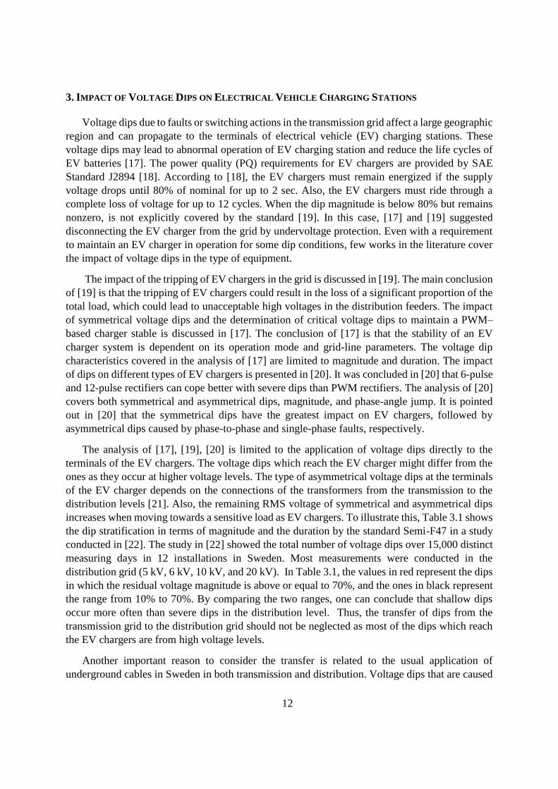
the distribution grid through which the voltage dip propagates. To illustrate the transient

propagation, Fig. 3.1 (left) shows a real voltage dip measured in 220 kV transmission grid

composed of a mix OHL-cable. The voltage dip contains a transient of 1 kHz at the dip starting at

which magnitude is about 1.239 p.u. Fig. 3.2 (middle) shows the propagation of the dip in 220 kV

to a distribution grid with feeders composed of cables with a length of 1.38 km, R=0.13 Ω/km,

L=0.32 mH/km, and C=0.47 µF/km [23]. Considering 13 feeders, the resonance frequency of the

equivalent cable is the same as the oscillation frequency of the transient at the voltage dip starting.

This way, the oscillation in the transient was amplified and reached 1.718 p.u. The same inference

can be obtained in Fig. 3.2 (right) which compares the spectra of the dip in 220 kV and 10 kV in

the first cycle. The magnitude of the component at 1 kHz is 15 times higher in 10 kV than 220 kV.

Fig. 3.1 Measured dip: Dip in 220 kV (left), Dip in 10 kV (middle), and Spectra (right).

In addition to that, faults in cables in the transmission grid might lead to phase-angle jumps

depending on the cable X/R ratio. The combination of the amplified transient and phase-angle

jump (PAJ) in the dips might make the EV charging stations to experience anomalous behavior

even for shallow dips. To evaluate this behavior, a study was conducted in equivalent system

presented in [23], considering voltage dips in 130 kV and their propagation to voltage levels of 10

kV and 0.4 kV. The model for the station was based on [24] which comprise of buck/boost dc-dc

converter and voltage source converter. The model for the distribution grid considers an equivalent

of 25 feeders composed of cables with a length of 1.38 km, R=0.13 Ω/km, L=0.32 mH/km, and

C=0.47 µF/km. Two types of voltage dips with 80% of magnitude and 0.1 s duration were applied

in 130 kV: one symmetrical (type A) and the other asymmetrical (type C). For both, two distinct

dip models with the transient frequency equal to the resonance frequency of the cable in 10 kV

14

(500 Hz): (i) zero PAJ; (ii) PAJ=20°. In all scenarios, the behavior of the EV station was analyzed

during the charging and discharging operation (injecting active power into the grid). For both

operations, three scenarios of active power were considered before the dip: (i) 0.35 MW, (ii) 0.7

MW, and (iii) 1.05 MW. The behavior of the EV station was analyzed in terms of dc-link voltage.

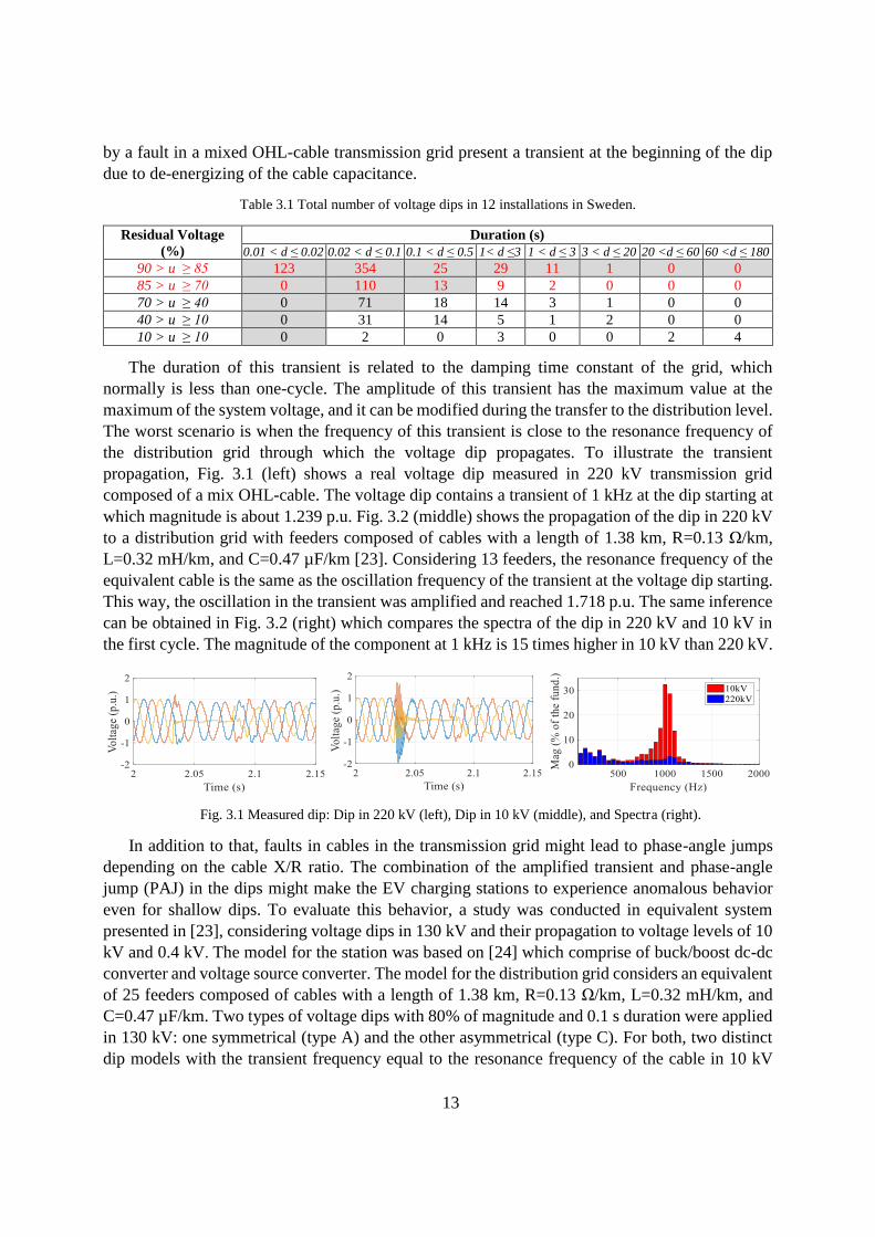
Fig. 3.2 shows the results for the dc-link voltage when the EV station is subjected to a voltage

dip type A. If the EV station is in the charging mode, the distinct scenarios for active power do not

affect the behavior of the dc-link. For the three active power scenarios, the overvoltage reached

1.1 p.u. On the other hand, the dc-link behavior was distinct among the active power scenarios

when the EV station is in the discharging mode. The overvoltage at the starting and during the

voltage dip is higher for the cases of 0.35 MW than the cases of 0.7 MW and 1.05 MW. For both

charging and discharging, the behavior is the same for the voltage dip with a PAJ of 20°.

Fig. 3.2 dc-link voltage for type A dip: charging (left) and discharging (right).

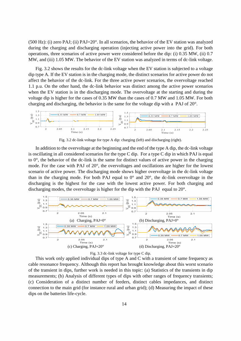
In addition to the overvoltage at the beginning and the end of the type A dip, the dc-link voltage

is oscillating in all considered scenarios for the type C dip. For a type C dip in which PAJ is equal

to 0°, the behavior of the dc-link is the same for distinct values of active power in the charging

mode. For the case with PAJ of 20°, the overvoltages and oscillations are higher for the lowest

scenario of active power. The discharging mode shows higher overvoltage in the dc-link voltage

than in the charging mode. For both PAJ equal to 0° and 20°, the dc-link overvoltage in the

discharging is the highest for the case with the lowest active power. For both charging and

discharging modes, the overvoltage is higher for the dip with the PAJ equal to 20°.

(a) Charging, PAJ=0° (b) Discharging, PAJ=0°

(c) Charging, PAJ=20° (d) Discharging, PAJ=20°

Fig. 3.3 dc-link voltage for type C dip.

This work only applied individual dips of type A and C with a transient of same frequency as

cable resonance frequency. Although this report has brought knowledge about this worst scenario

of the transient in dips, further work is needed in this topic: (a) Statistics of the transients in dip

measurements; (b) Analysis of different types of dips with other ranges of frequency transients;

(c) Consideration of a distinct number of feeders, distinct cables impedances, and distinct

connection to the main grid (for instance rural and urban grid); (d) Measuring the impact of these

dips on the batteries life-cycle.

15

4. IMPACT OF EV CHARGING FAST VOLTAGE FLUCTUATIONS ON LIGHT FLICKER

EV charging would create fast voltage fluctuations whose magnitude depends on the transient

charging current peak and impedance of the grid. This fast voltage fluctuation could create light

flicker (repetitive change in light intensity) that human can perceive. The current peak depends on

the state of the charge (SOC) of the EV. The SOC depends on the ambient temperature and on the

battery’s age and capacity. It makes the SOC unpredictable and therefore the current peak too. The

current peak could reach up to 16 A in common household low voltage networks.

The charging of EVs can be fast or slow. The current patterns obtained with fast charging and

slow charging are different as more fluctuations were found in slow charging. Fast voltage

fluctuations could be found at the beginning and at the end of the charging cycle. Similarly, battery

status check, insulation test for output dc circuit, on board battery protection, voltage checks, CAN

communication interval for charging current request, etc. can also create fast voltage fluctuations

in both slow and fast charging [25], [26]. The present study is focuses on household chargers which

are usually slow charging.

The transfer impedances of an 83 customers network of Northern Sweden are calculated. The

maximum transfer impedance value obtained between customer was between 0.0496 Ω to 0.3512

Ω (strong grid). The current peaks applied to the transfer impedances are from 1 A to 16 A

considering steps of 1 A. The voltage drops obtained are up to 5.5 V rms. The 90% of the voltage

drops obtained are below 3.5 V rms and the 50% below 1 V rms. It shows that in general this

network is a suburban as known also from the transfer impedance values. To extent this study for

a similar weak grid the impedance of 59468 customers network was obtained. The 90% of the

impedances are below 0.3638 Ω (similar to the maximum impedance obtained in the 83 customers

network) and 99% were below 0.6895 Ω. Applying the same currents peaks as before, the

maximum voltage drop obtained for 0.6895 Ω (weak grid) is 11 V.

Since the EV connection is random, the flicker can appear whenever along the 10 min that the

light flickermeter uses to measure the level of annoyance (Pst, meaning Pst=1 that in 50% of the

cases flicker is experienced by an average observer). A previous study [27] estimated the

probability of the number of steps in the current due to EV charging that could take place along 10

min depending on the number of vehicles charging at the same time is shown in Table 4.1.

Table 4.1 Probability of more than a given number of changes in light intensity during a

10-minute interval, as a function of the number of electric vehicles charging electrically nearby.

Number of vehicles charging at the same time

Number of steps 3 4 5 6 7 8 9 10 20 50 80

>2 4% 11% 21% 32% 43% 53% 62% 70% 98% 100% 100%

>3 1.0% 4.5% 10% 17% 26% 35% 44% 94% 100% 100%

>4

>10

>20

>30

0.4% 1.8% 4.5% 8.8% 14.5% 21% 84%

3.5%

100%

96%

12%

100%

100%

95%

23%

The Pst is obtained applying 5.5 V, 7 V and 11 V of voltage drop to a set of 32 LED lamps

from 3 to 11 W. Table 4.2 shows the Pst of 4 LED lamps sorted from the least (LED 1) to the most

16

affected (LED 4). LED 2 and 3 shows two representative Pst values of the set of lamps. LED 1, 2

and 4 point to an active power factor correction (APFC) topology and LED 3 to a dimmable lamp

with a capacitive topology attending to the author criteria considering the current waveform shape.

According to Table 4.1, 4 number of steps (current peaks) is the highest with 100% of

probability due to EVs charging considering that there are 50 EVs and 10 number of steps while

considering 80 EVs. For further analysis 4 and 10 number of voltage drops within 10 minute

interval is considered. These drops were investigated by applying test patterns in consecutive steps

(the instantaneous flicker from the first step hasn’t dropped when the second step occurs) and in

non-consecutive steps. The results in Table 4.2 show the Pst exclusively due to the voltage drops,

therefore the Pst obtained when there is no voltage drops (Pst of the background distortion) for each

lamp has been subtracted from the measured value.

Table 4.2. Light-Pst for 4 and 10 voltage drops of different magnitude distributed consecutively and non-

consecutively.

Pst of Consecutive drops Pst of Non-consecutive drops

Weak grid

(11 V)

Medium grid

(7 V)

Strong grid

(5.5 V)

Weak grid

(11 V)

Medium grid

(7 V)

Strong grid

(5.5 V)

4 drops

LED 1 0.2336 0.1278 0.0910 0.1936 0.1025 0.0702

LED 2 0.4012 0.2408 0.1836 0.2893 0.1726 0.1309

LED 3 0.5745 0.3386 0.2610 0.4169 0.2574 0.1981

LED 4 1.0925 0.6888 0.5255 0.7909 0.4845 0.3620

10 drops

LED 1 0.4077 0.2289 0.1663 0.2498 0.1362 0.0949

LED 2 0.6655 0.3971 0.3023 0.3846 0.2307 0.1745

LED 3 0.9321 0.5586 0.4183 0.5386 0.3287 0.2505

LED 4 1.8493 1.1804 0.9075 1.0415 0.6436 0.4830

Since the consecutive voltage drops considered take place in the visibility range according to

IEC 61000-3-7 standard [28], the Pst values are higher for this distribution. Considering non-

consecutive drops, the maximum Pst variations between LED lamps are around 0.6 and 0.8

considering 4 and 10 drops respectively in a weak grid and around 0.3 and 0.4 respectively in a

strong grid. Considering consecutive drops the variations are around 0.85 and 1.4 considering 4

and 10 drops respectively in a weak grid and around 0.4 and 0.75 respectively in a strong grid. It

means that the difference in Pst between LED lamps increase with level of voltage magnitude

variations.

The differences in Pst between a weak and strong grid for LED 1 (least affected) and LED 4

(most affected) are around 0.14 and 0.57 respectively considering 4 consecutive drops and around

0.24 and 0.95 respectively considering 10 consecutive drops. The variation in the Pst between LED

lamps connected to the same grid can be bigger than the variation in the Pst when an LED lamp is

connected to different grid impedances.

The Pst is below 1 for the majority of the set of LED lamps under the distortions considered.

Only for LED 4, the most affected, the Pst is over 1 in a weak grid when 4 consecutive drops or 10

(consecutive or non-consecutive) drops take place and in a medium grid when 10 consecutive

drops take place (cells with red borders). Therefore, the flicker due to EVs charging may be a

problem depending on the number of EVs connected (number of voltage steps), pattern of voltage

steps (consecutive), LED lamps used by the customers and the impedance of the grid.

17

5. IMPACT OF EV CHARGING ON NEUTRAL AND PROTECTIVE EARTH

The impact of electric vehicle chargers on the neutral and protective earth current and their

consequences are discussed in this section. Single-phase rectifier in EV home chargers emanate

third harmonic component in the neutral conductor. The PWM switching methods are used to

reduce the lower order harmonics in the system. These chargers usually switch in the

supraharmonics frequency range. Multiple chargers connected as residential loads, lead to an

increase in the supraharmonics in the neutral and protective earth conductors. This can have

adverse effect on the operation of residual current devices (RCD) or ground fault interrupters

(GMI). The increase in the leakage current (PE current due to supraharmonics) and triplen

harmonics can increase the RMS value of neutral current and cause false tripping of RCDs. Neutral

conductor can act as spreader of supraharmonics to the other loads connected in parallel with EV

chargers [29]. The measurements of leakage current for several household appliances shown in

[30] conclude that the equipment such as EVs, PVs and battery chargers create high leakage

currents, leading to a higher probability of RCD tripping. In [31] authors suspect the reason for

RCD tripping multiple times per week as the amplitude beating in phase currents and voltages

caused by the differences in the switching frequencies of same type of EVs connected in the same

phase combined with supraharmonic emission. The author in [32] through measurement shows the

accumulation of “high frequency noise” caused by the EV charger on the charge circuit

interrupting device (CCID). This is superimposed on the 60 Hz signal causing high leakage current,

resulting in the tripping of CCID. Users of EV in Sweden have reported interruptions in the EV

charging process for high levels of supraharmonics in the neutral-to-protective earth (N-PE)

voltage [27]. Norway uses IT earthing system, where the equipment is grounded separately at the

user end and has no connection to the neutral wire coming from the utility [33]. The ground fault

interrupters (GMI) in EV are used to detect ground fault and disconnect the charger to protect the

humans from shock in case of fault. The article [33] reported issue that has not yet been examined

is fuse tripping even when the EV is not charging at home charging stations. This may be due to

poor filter or charging system design, and possibly due to leakage current through resistors

connected between phase to earth.

The supraharmonics in neutral current are instantaneous summation of the three-phase currents

[34]. Measurements were made in the Per Högstrom laboratory for a single-phase EV. The

measured single-phase current was used to make three-phase current shifting the measured phase

current by one third of one cycle at power-system frequency. It is assumed that the load is

homogenous and balanced with three-phase four-wire connection. The supply voltage is assumed

balanced and non-distorted.

A plug-in hybrid vehicle (88 kW rated power) with light flicker complaint while charging was

chosen for further analysis. The battery has 28 kWh capacity, which gives an range of 195 km.

The battery charger is rated 6.6 kW. The supraharmonic emission of this EV is in the range of 45

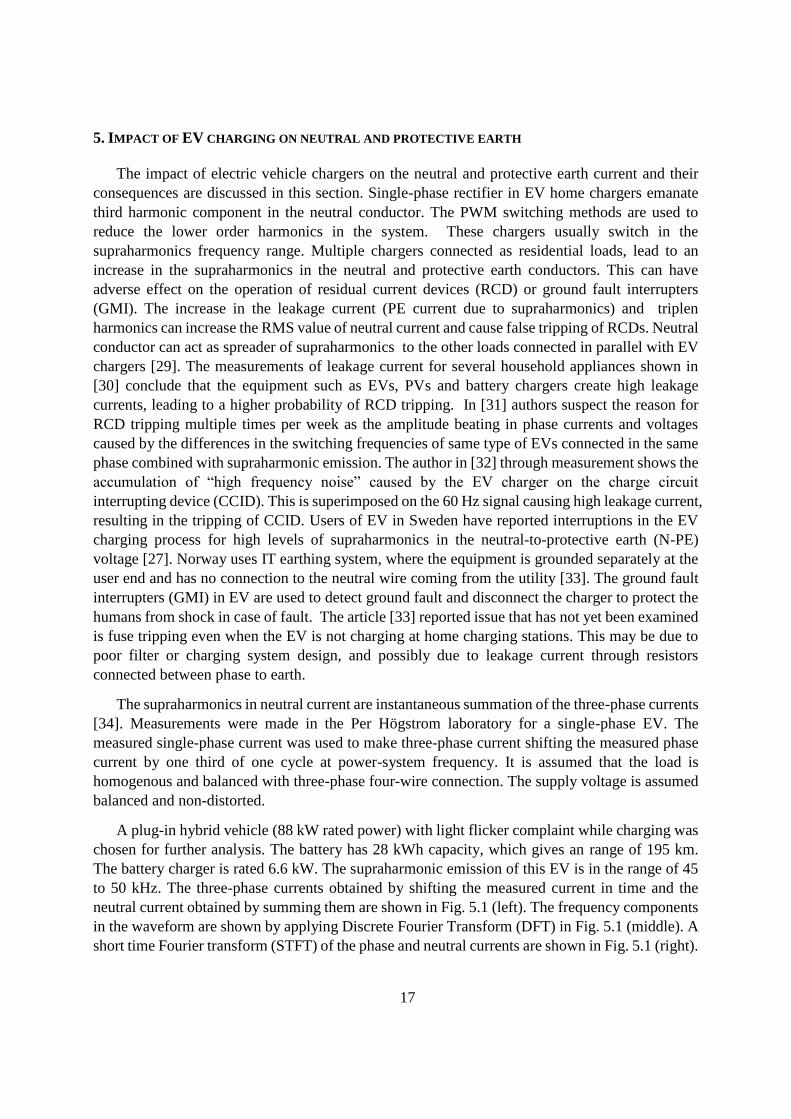
to 50 kHz. The three-phase currents obtained by shifting the measured current in time and the

neutral current obtained by summing them are shown in Fig. 5.1 (left). The frequency components

in the waveform are shown by applying Discrete Fourier Transform (DFT) in Fig. 5.1 (middle). A

short time Fourier transform (STFT) of the phase and neutral currents are shown in Fig. 5.1 (right).

18

The STFT shows the variation of supraharmonics in time. The summation of supraharmonics in

neutral can be seen in the neutral current.

(a) (b)

(c)

Fig. 5.1 (a) Time-domain, (b) frequency-domain and (c) time-frequency-domain representation of the three-phase

measured EV current.

The emission from EV range is quantified using total supraharmonic emission current (TSHC)

defined in [35]. To predict the emission of supraharmonics in phase and neutral conductors, the

equation defined in [36] is used to mathematically model total supraharmonics current flowing

into the grid per phase according to the number of devices connected. The author in [34] modified

this equation for neutral conductor. The modification was based on the hypothesis that the number

of equipment seen by the neutral at a given instant is three times that connected to the phase

conductors. The change in the magnitude of supraharmonics in neutral w.r.t change in number of

devices connected per phase is given by (5.1) [34].

𝑅𝑛𝑝 =𝐼𝑛

𝐼𝑝ℎ=

√3∗ √1+𝑁2𝛼2

√1+(3∗𝑁)2𝛼2 (5.1)

where 𝛼 = 𝜔𝑅𝐶, N = number of equipment connected as load, 𝐼𝐿 = TSHC of the measured

current flowing to the grid from one EV = 76.3 mA, 𝑅 = resistance calculated at the point of

19

connection (PoC), C = capacitance calculated at PoC. The value of α depends on the relationship

between the grid impedance and load impedance, thus the values of R and C should be calculated

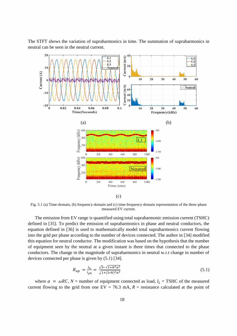
at the PoC. α is calculated as 0.10 from the measurements for the EV [37]. Fig. 5.2 (left) shows

that the phase TSHC increases for certain number of EV and then starts decreasing. The neutral

TSHC starts decreasing much before the phase TSHC. This is because the neutral conductor sees

all the three phases connected at the same time, thus it sees three times the number of EV. Fig. 5.2

(right) shows the rate at which neutral TSHC decreases as compared to phase TSHC.

Fig. 5.2 Phase and neutral current supraharmonic emission (left) and Change in the ratio (right).

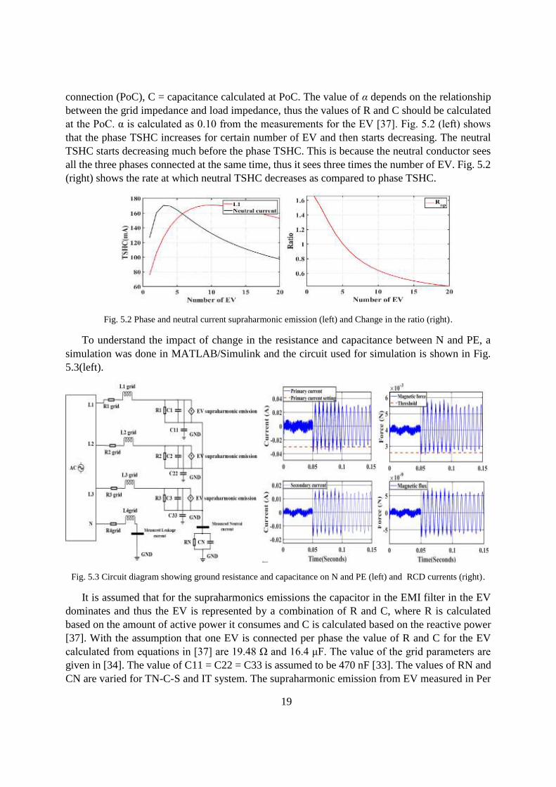
To understand the impact of change in the resistance and capacitance between N and PE, a

simulation was done in MATLAB/Simulink and the circuit used for simulation is shown in Fig.

5.3(left).

Fig. 5.3 Circuit diagram showing ground resistance and capacitance on N and PE (left) and RCD currents (right).

It is assumed that for the supraharmonics emissions the capacitor in the EMI filter in the EV

dominates and thus the EV is represented by a combination of R and C, where R is calculated

based on the amount of active power it consumes and C is calculated based on the reactive power

[37]. With the assumption that one EV is connected per phase the value of R and C for the EV

calculated from equations in [37] are 19.48 Ω and 16.4 μF. The value of the grid parameters are

given in [34]. The value of C11 = C22 = C33 is assumed to be 470 nF [33]. The values of RN and

CN are varied for TN-C-S and IT system. The supraharmonic emission from EV measured in Per

20

Högstrom laboratory shown in Fig. 5.1 is used as input to the current source in Fig. 5.3 (left). RCD

model using summing transformer (modelled through inductance) and an electromagnetic relay

developed in [38] is used in this study. The leakage current measured from the circuit in Fig. 5.3,

is given as input to the RCD model. An RCD is characterized by its rated residual operating current

𝐼∆𝑁 (typically 30 mA in a low-voltage installation). It can also be differentiated according to the

time it trips, i.e., an RCD can trip instantaneously when the 𝐼∆𝑁 is reached.

Two cases are considered one with RN = 20 kΩ and CN = 100 μF [33], for IT system and RN

= 1Ω, CN = 220nF for TN-C-S system. For both cases, a background voltage distortion from 0.05

to 0.15 second with 3rd harmonic being 0.002 pu, 180° and 5th harmonic 0.015 pu and 35° is

superimposed on the grid voltage. By changing the values of RN and CN, it was concluded that

with low value of capacitance the leakage current decreases, whereas with low value of resistance

it increases. For a TN-C-S system, the value of resistance is usually low leading higher value

leakage current for the same device. The value of capacitance CN depends on the device connected.

In an installation with high value of capacitance and low value of resistance, the leakage current

would be the highest. EVs connected at such installations can contribute highly to the leakage

current. Fig. 5.3 (right) shows the behaviour of the leakage current obtained from the case

emulating TN-C-S system. For 0 to 0.05 seconds, the primary winding of the RCD sees only the

leakage current, which is below the trip current setting of the RCD. When the background voltage

distortion is applied at 0.05 seconds, the primary current reaches the tripping limit. The magnetic

force generated is enough to trip the RCD. From 0.1 seconds the supraharmonics are absent and it

can be seen that the force needed to trip the RCD reduces even though the magnitude of primary

current is approximately equal to the trip current. The presence of supraharmonics increases the

risk of RCD tripping. The tripping of RCD due to only supraharmonics, would need the worst case

scenario with multiple EVs charging where the supraharmonics in neutral conductor are still

summing.

21

6. PV – EV HOSTING CAPACITY ASSESMENT IN VIEW OF UNDERVOLTAGE

The hosting capacity for electric vehicles in a low-voltage distribution network considering the

undervoltage phenomenon can be quantified by analysing the pattern of driving; charging

characteristics, time of charging and the penetration level.

A stochastic approach is developed for estimating the hosting capacity of electric vehicles charging

in a low-voltage distribution network considering the undervoltage which was initially developed

for the integration of solar PV to low-voltage networks [39]. The estimate of the voltage drop due

to electric vehicle (EV) charging at a customer and eventually likely to cause an undervoltage

phenomenon is estimated using equation (6.1).

∆𝑈 (𝑎) = 𝑍𝑡𝑟(a, b) × (−𝐼𝐶𝑢𝑠𝑡(b) − 𝐼𝐸𝑉(b)) (6.1)

Where ∆𝑈 (𝑎) is the complex voltage drop at the customer (compared to the no-load

situation), 𝑍𝑡𝑟(a, b) is the source impedance for the customer, 𝐼𝐶𝑢𝑠𝑡(𝑏) are the customers non-EV

current demand and 𝐼𝐸𝑉 (b)is the electric vehicle charging current demand at a customer.

The voltage during EV charging can be estimated using equation (6.2), the minus sign depicts

the customers' non-EV power consumption and the EV charging power consumption

U (a) = 𝑈0(a) + ∑ 𝑍𝑡𝑟(a, b) (−𝐼𝐶𝑢𝑠𝑡(b) − 𝐼𝐸𝑉(𝑏))𝑁𝑏=1 (6.2)

Where; 𝑍𝑡𝑟 is the transfer impedance, 𝐼𝐶𝑢𝑠𝑡(𝑏) is the customers' current (high power

consumption), 𝑈0 (a)is the background voltage during high load conditions and, 𝐼𝐸𝑉(𝑏) is the

current as a result of electric vehicle (EV) charging.

In equation (6.2), the background voltage (𝑈0 (a) ) is introduced for estimating the voltage

magnitude change due to electric vehicle charging. The lowest customer voltage is expected during

the periods of high customer consumption. This is the background voltage during the period of

interest which is later on defined as the time-of-day (ToD). The highest impact from the electric

vehicle charging on the voltage level is expected to be during this background voltage (𝑈0 (a)).

The following time-of-day (ToD) are considered for the stochastic approach:

The day-time (ToD-I) charging defined for the time range from 06 am to 06 pm.

The night-time (ToD-II) charging defined for the time range from 06 pm to 06 am.

The study of the interaction between electric vehicles and solar PV is done when there is the

presence of both sources at a customer. The ratio of the number of times that the two are present

at a customer is referred to as the coincidence factor of EV and solar PV. The coincidence factor

is estimated using equation (6.3) [40].

𝐶𝐸𝑉−𝑃𝑉 =𝑃𝑃𝑉 𝑜𝑓 𝐼𝑛𝑐𝑖𝑑𝑒𝑛𝑡 (𝑇𝑖𝑚𝑒−𝑜𝑓−𝑑𝑎𝑦)

𝑃𝐸𝑉 (𝑇𝑖𝑚𝑒 𝑐𝑜𝑛𝑠𝑖𝑑𝑒𝑟𝑒𝑑) (6.3)

Where; 𝑍𝑃𝑃𝑉 is the solar PV power incident with the electric vehicle charging power 𝑃𝐸𝑉 is

during the time of day (ToD-I) considered for the impact.

The impact of solar PV on the effect of an electric vehicle charging is significant when there

is a high coincidence factor, and more customers are charging. The coincidence factor is indicative

of the how much solar PV power influences the voltage level in a distribution network in the

22

presence of electric vehicles. The voltage level due to customer electric vehicle charging in the

presence of solar PV is estimated using equation (6.4).

U (a) = 𝑈0(a) + ∑ 𝑍𝑡𝑟(a, b) (−𝐼𝐶𝑢𝑠𝑡(b) − 𝐼𝐸𝑉(𝑏) + 𝐼𝑃𝑉(𝑏))𝑁𝑏=1 (6.4)

Where; 𝑍𝑡𝑟 is the transfer impedance, 𝐼𝐶𝑢𝑠𝑡(𝑏) is the customers' current (high power

consumption), 𝑈0 (a) is the background voltage during high load conditions, 𝐼𝐸𝑉(𝑏) is the current

as a result of electric vehicle (EV) charging and 𝐼𝑃𝑉(𝑏) is the current as a result of solar PV power

injection at the customer.

The distribution network used in this study has 83-customers. The lowest number of customers

from 6 am to 6 pm is estimated to be 17-customers (20%). During the daytime, at least 20% of the

customers have a high likelihood to charge their electric vehicles i.e. population above 65 years

[41]. Other penetration levels are also possible when taking into account other customers below

65-years who are arriving at home and charging their electric vehicle load. The possibility is

illustrated with the arrival time characteristic shown in Fig. 6.1.

The electric vehicles consumption profiles are provided for 348-EVs at 200 sampled houses

[42]. In addition to the power levels in [42], the comprehensive list of the charging levels used to

estimate the hosting capacity is shown in Table 6.1.

Table 6.1 Single-phase and three-phase electric vehicle charging power applied

Level 01 02 03 04 05 06 07 08 09 10

1 -Phase: 1.92 2.3 3.68 4.6 5.75 8.05 9.2 11.5 14.49

3 -Phase: 3.3 4.6 6.9 11.04 13.8 17.25 24.15 27.6 34.5 43.47

A stochastic approach with Monte-Carlo simulation has been used to calculate the probability

distribution functions of the voltage (with EV charging) for each of the customers and obtain the

10th percentiles of the resulting voltage level applying equations (6.3) and (6.4). As a default,

400000 samples are used for the calculation. The hosting capacity is exceeded when the 10th

percentile value obtained is below 90% of the nominal voltage (230V) for atleast one of the

customers.

The electric vehicle arrival time is the hour of the day that it returns home from a trip and starts

charging [43], [44]. Higher probability of customers arriving home is around 6 pm as per Fig.

6.1(left) [44], [45]. The customer consumption profile at 10-minute average of a town in northern

Sweden is shown in Fig. 6.1 (right). The mean value of consumption for the two measurements is

1062 and 1001 W for the ToD-I (black) and ToD-II (red). There is a difference of 61 W.

Fig. 6.1 Arrival time for EVs in residential area (left) and customer power consumption with the background voltage

during the ToD-I and ToD-II (right)

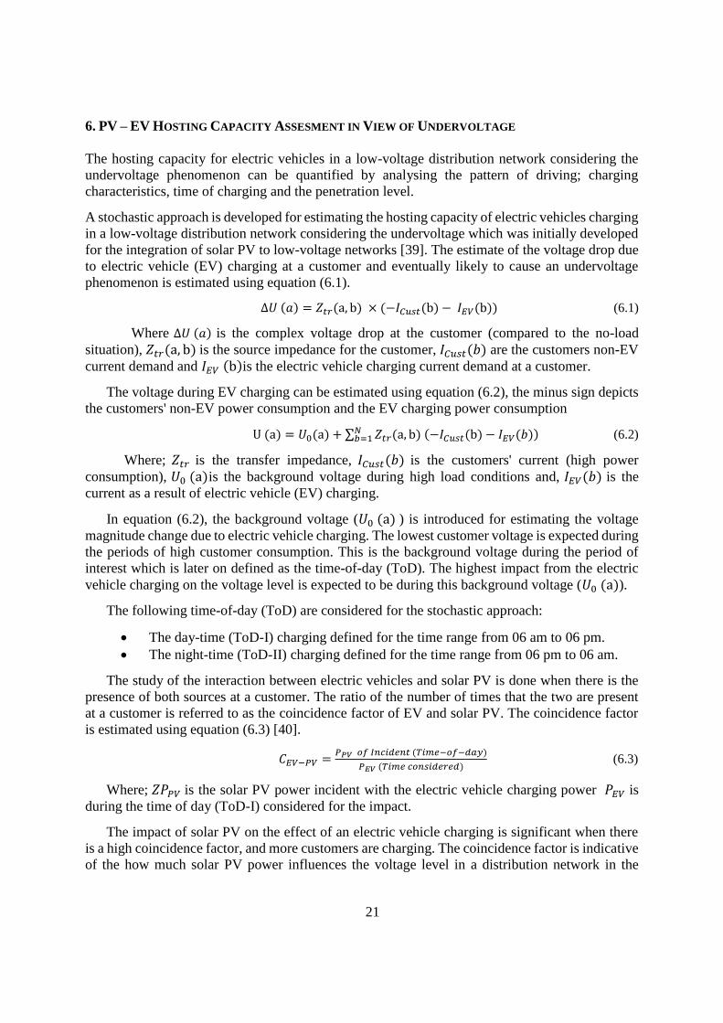
The input background voltages for ToD-I and ToD-II are shown in Fig.6.2.

23

Fig. 6.2 Applied background voltage of measurements during the ToD 06 am – 06 pm (Daylight) (left) and 06 pm –

06 am (Night) (right).

The input background voltage of all the measurements for the ToD-I varies in the range 226.93-

233.81 V and for ToD-II between 227.66-233.96 V. The results obtained in Figure 6.2 are

comparative for the measurements applied. For measurements in other distribution networks, the

background voltage for the defined ToDs can be comparatively similar or not. The loading aspect

and the tap-changer position or operation can influence the obtained values.

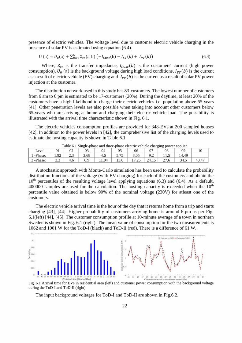
The hosting capacity results for 20 % penetration (percentage of the customers) during the

ToD-I for single-phase chargers are shown in Fig. 6.3.

Fig. 6.3 Single-phase hosting capacity results for the applied background voltage during (ToD-I).

Single-phase hosting capacity is 100 % for all the 17-customers likely to charge at 20 %

penetration during the ToD-I shown in Fig. 6.3 (left). The likelihood of an undervoltage violation

is low for 5-charging power levels (1.92-5.75 kW). There is a likelihood of an undervoltage for

the charging power level of 8.05 kW. The impact is even severe for 9.2, 11.5 and 14.49 kW

charging levels. During the daytime and 20 % penetration level, the single-phase hosting capacity

varies between 7-17 customers, as shown in Fig.6.3.

The hosting capacity results for the customers during the ToD-I for three-phase chargers are

shown in Fig. 6.4. Three-phase hosting capacity is 100 % for 7-charging levels shown in Fig. 6.4

(3.3-24.15 kW). The charging levels of 27.6, 34.5 and 43.45 kW show a variation of hosting

capacity between 10-17 customers.

24

Fig. 6.4 Three-phase hosting capacity results for the applied background voltage during (ToD-I).

The hosting capacity results for the customers (100 % penetration) during the ToD-II for

single-phase chargers are shown in Fig. 6.5. The single-phase hosting capacity shows variation for

all the 9-charging levels assessed in Fig. 6.5. The hosting capacity is between 10-83 customers for

5-charging levels up to 5.75 kW. Above 5.75 kW charging level, the hosting capacity is 2-14

customers.

Fig. 6.5 Single-phase hosting capacity results for the applied background voltage during (ToD-II).

The hosting capacity results for the customers during the ToD-II for three-phase chargers are

shown in Fig. 6.6. Three-phase hosting capacity obtained is between 45-83 customers for the first

three charging levels, i.e. 3.3, 4.6 and 6.9 kW. For the 3.3 kW charging level, all the customers

can charge without affecting the undervoltage limit. Considering six charging levels covering 3.3

to 17.25 kW, the hosting capacity varies between 15-customers and 83-customers.

Fig. 6.6 Three-phase hosting capacity results for the applied background voltage during (ToD-II).

For the next charging levels, the hosting capacity varies between 3-customers and 22-

customers—the likelihood of an undervoltage increases for the charging power of 24.14 kW to

43.47 kW.

25

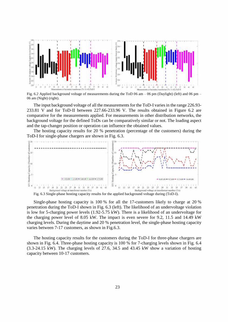
The impact of solar PV on the electric vehicle hosting capacity with 20 % penetration was

assessed. A 3 kW single-phase solar PV plant is applied to the single-phase charging power levels

of 8.05, 9.2, 11.5 and 14.49 kW. The results obtained are shown in Fig. 6.7. Solar PV injection at

a customer increases the voltage level and hence the hosting capacity [39]. The results shown in

Fig. 6.7 (left) illustrates the phenomena. Further assessment was done with a 6 kW single-phase

solar PV unit. At 20 % penetration level, all the customers (17) did not violate the undervoltage

limit.

(a) (b) (c) (d)

Fig. 6.7 EVs hosting capacity obtained without and with 3 kW solar PV at 20% penetration level during ToD-I.

Note: single phase (a & b) and three phase (c & d)

An assessment of a 3-phase solar PV charging for power levels of 27.6, 34.5 and 43.37 kW

was also done. The results obtained with a 3 kW three-phase solar PV unit are shown in Fig. 6.7.

The hosting capacity increases for two of the three charging levels considered. The additional

assessment was done for the 6 and 9 kW three-phase solar unit. The results obtained with 9 kW

solar PV units allows all customers at 20% penetration to charge using a maximum of 43.47 kW.

The following are concluded from the results obtained for both time-of-days (ToD-I and ToD-II).

There is a need to keep track and monitor the penetration of electric vehicles in distribution

networks.

During the day time (6 am – 6 pm), the impact of electric vehicles is lesser than the impact

during the night time (6 pm – 6 am) considering the 20% penetration level of electric

vehicles likely to be charging. The impact is also dependent on the coincidence factor. The

impact in the day could be similar to the night time for penetration levels greater than 20%

The impact of solar PV on electric vehicle hosting capacity during the day depends on the

coincidence factor, the time both are interacting.

For the case considered, 20% penetration level during the day time and based on the

assumption made, the likelihood for an undervoltage for single-phase 6 kW and three-

phase 24 kW is almost low.

The likelihood of an undervoltage violation is high during the night time and for larger

penetration levels during daytime.

Three-phase charging power presents a lesser likelihood than single-phase chargers.

The following work is needed in future:

More measurements and obtaining background voltage for the two defined ToDs.

Application of the method to aggregated MV-LV distribution networks.

26

7. ENHANCEMENT OF GRID CAPACITY FOR EV CHARGING USING DYNAMIC LINE RATING

With an increase in the number of EV charging the management of corresponding demand

should be carefully aligned with the available resources [46], [47]. Though the long term solution

is to increase the grid capacity by upgrading the infrastructure, the practical solution is to develop

a smart and flexible technique to aid power grid operation through dynamic line rating (DLR). In

the regional grid the thermal capacity based on worst case weather condition is used to fix the

transfer capacity for the entire year, which results in under utilization of available capacity for

most hours of the year. Northern Sweden experience peak load during winters, the fixed line rating

would set limit to the amount of vehicle charging that can be connected to the grid.

As per IEEE Std 738-2012 [48], the capacity of a transmission line is dynamically varying

according to the environmental conditions and line behaviour as per (7.1) while using DLR.

𝑞𝑠 + 𝑞𝑗(𝑇𝑐, 𝐼) = 𝑞𝑠(𝑇𝑐, 𝑇𝑎, 𝑉𝑚, 𝜑) + 𝑞𝑠𝑐(𝑇𝑐, 𝑇𝑎) (7.1)

Where 𝑞𝑐 , 𝑞𝑟 , 𝑞𝑠 and 𝑞𝑗 are convection heat loss, radiation heat loss, solar heat gain and

joule heating, respectively. The magnitude of each of these terms is dependent on variables such

as conductor temperature, 𝑇𝑐, ambient temperature, 𝑇𝑎, wind speed, 𝑉𝑚, and wind angle attack, 𝜑.

The hosting capacity indicator is defined as the maximum number of cars, 𝑁𝐸𝑉 , that can get

connected at the same time in the whole local area and is given by (7.2),

𝑁𝐸𝑉 ≤𝑃𝑎𝑣𝑎𝑖𝑙𝑎𝑏𝑙𝑒

𝑃𝐸𝑉 (7.2)

Where 𝑃𝑎𝑣𝑎𝑖𝑙𝑎𝑏𝑙𝑒 is the available margin and 𝑃𝐸𝑉 is the charging station capacity.

The real-time analysis of the transferable capacity, in MW, for two cases with static and dynamic

rating is shown in Fig. 7.1. The static rating is assumed for 𝑇𝑎, 35ºC, 𝑉𝑚, 0 m/s and maximum

insolation.

Fig. 7.1. Real-time hosting capacity of the existing overhead line during the period between 2011 and 2018 (left)

fixed line rating and (right) dynamic line rating.

Due to low heating load during summer the potential of adding EVs to the grid is more than 10

MW or 50% of peak consumption. In winter when the temperature is very low the EV batteries

get discharged faster and hence need to be charged frequently resulting in overloading while using

static line rating. With dynamic rating the minimum capacity is 15 MW which is almost 75% of

the maximum transfer capacity with static rating as shown in Fig. 7.1 (right). The hosting capacity

reach up to 60 MW, this is not the usual case. On average the line can accept 35 MW during

working hours. There is a risk of overestimation or underestimation of thermal transfer capacity

while using DLR to increase the hosting capacity which may result in curtailment (disconnection

of part of the load) [49]. The overloading risk due to EV charging on the transmission and sub-

transmission network in northern Sweden during the period 2011 to 2018 was investigated. The

weather data are obtained from the Swedish Meteorological and Hydrological Institute (SMHI).

Under firm hosting capacity there is no considerable difference between the number of cars

charging during weeks and weekends. However, slightly more cars can get charged during nights

27

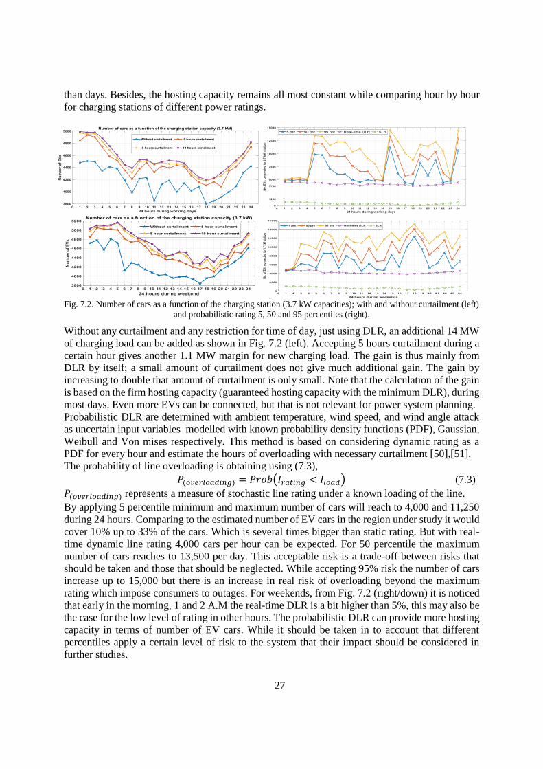
than days. Besides, the hosting capacity remains all most constant while comparing hour by hour

for charging stations of different power ratings.

Fig. 7.2. Number of cars as a function of the charging station (3.7 kW capacities); with and without curtailment (left)

and probabilistic rating 5, 50 and 95 percentiles (right).

Without any curtailment and any restriction for time of day, just using DLR, an additional 14 MW

of charging load can be added as shown in Fig. 7.2 (left). Accepting 5 hours curtailment during a

certain hour gives another 1.1 MW margin for new charging load. The gain is thus mainly from

DLR by itself; a small amount of curtailment does not give much additional gain. The gain by

increasing to double that amount of curtailment is only small. Note that the calculation of the gain

is based on the firm hosting capacity (guaranteed hosting capacity with the minimum DLR), during

most days. Even more EVs can be connected, but that is not relevant for power system planning.

Probabilistic DLR are determined with ambient temperature, wind speed, and wind angle attack

as uncertain input variables modelled with known probability density functions (PDF), Gaussian,

Weibull and Von mises respectively. This method is based on considering dynamic rating as a

PDF for every hour and estimate the hours of overloading with necessary curtailment [50],[51].

The probability of line overloading is obtaining using (7.3),

𝑃(𝑜𝑣𝑒𝑟𝑙𝑜𝑎𝑑𝑖𝑛𝑔) = 𝑃𝑟𝑜𝑏(𝐼𝑟𝑎𝑡𝑖𝑛𝑔 < 𝐼𝑙𝑜𝑎𝑑) (7.3)

𝑃(𝑜𝑣𝑒𝑟𝑙𝑜𝑎𝑑𝑖𝑛𝑔) represents a measure of stochastic line rating under a known loading of the line.

By applying 5 percentile minimum and maximum number of cars will reach to 4,000 and 11,250

during 24 hours. Comparing to the estimated number of EV cars in the region under study it would

cover 10% up to 33% of the cars. Which is several times bigger than static rating. But with real-

time dynamic line rating 4,000 cars per hour can be expected. For 50 percentile the maximum

number of cars reaches to 13,500 per day. This acceptable risk is a trade-off between risks that

should be taken and those that should be neglected. While accepting 95% risk the number of cars

increase up to 15,000 but there is an increase in real risk of overloading beyond the maximum

rating which impose consumers to outages. For weekends, from Fig. 7.2 (right/down) it is noticed

that early in the morning, 1 and 2 A.M the real-time DLR is a bit higher than 5%, this may also be

the case for the low level of rating in other hours. The probabilistic DLR can provide more hosting

capacity in terms of number of EV cars. While it should be taken in to account that different

percentiles apply a certain level of risk to the system that their impact should be considered in

further studies.

28

8. DISTRIBUTION TRANSFORMER OVERLOADING DUE TO EV INTEGRATION: A STOCHASTIC APPROACH

The fast chargers are considered as a practical and efficient method to ease the concerns of

long charging durations, thus the number of fast charging stations are increasing rapidly in recent

years. Therefore, the overloading possibility of the distribution transformers is also increasing with

increasing number of fast charging facility and EVs. Due to increasing EV penetration there is an

outage probability due to power supply capacity shortage of the distribution transformers.

The actual load profile of a distribution transformer of a Northern city in Sweden is considered

for the use-case. Meanwhile, the EV charging profile of the parking lot is generated in a stochastic

way based on real charging profile of seven different charging stations of the same city. It is

important to mention that the aggregated charging pattern of the EV charging stations is prioritize

over the charging pattern of a specific station, because that has higher impact on overall

overloading of the distribution transformer. Numerous studies have been carried out to investigate

the impact of EV deployment on load profile [52], [53]. Meanwhile, the impacts of the EVs on

distribution transformers are investigated and reviewed in [54]-[56]. The impact of EV charging

on distribution cable or line loading are reflected in some recent studies [57], [58]. Moreover, the

location of the EV charging stations changes the dynamic load flow characteristics of the

distribution network sometimes that causes additional power losses, hence, additional power

demand from distribution transformers. Such study has been carried out for a typical Danish

distribution network with EV penetration rates up to 50% [59]. For the EV adoption rate of 50%,

the system losses increase 40% compared to the base case in the uncontrolled EV charging scenario.

However, most of these study consider deterministic approaches to model the EV charging profile

for the concerning study, while it is challenging also to model the EV charging characteristics in a

stochastic approach.

The dynamic behaviors of EV charging, such as random charging time, charging duration and

vehicle charging locations are modelled using a Monte-Carlo simulation to analyze the harmonics

and voltage profile in [60], [61]. Meanwhile, the charging time, charging duration, and required

amount of energy as stochastic parameters are more important than charging location for this study

to analyze the overload possibilities of the distribution transformer. The stochastic charging and

discharging pattern of individual EV are shown in [62], [63]. As it is explained earlier, this study

is focused on the aggregated charging profile of EV charging stations thus a Markov chain Monte

Carlo simulation (MCMCS) model is used to simulate the stochastic energy demand of EVs in

time series.

The Markov chain model is a stochastic model that creates samples randomly based on a

particular sequential process. The MCS model is one of the most used methods which

systematically generates samples from a random process by considering the probability

distribution function (PDF) of uncertain variables. The MCS model generates a well-defined

distribution function, which ensures a high correlation between the histograms of historical data

and generated samples. Nonetheless, it cannot explain the time-dependency and continuity

between generated values and the long-term behavior of uncertain variables. The MCMCS has an

iterative process which works as follows [64]:

Consider 𝜃 as a current state. For each iteration, a random value, 𝜃 is generated.

The decision about the acceptance of 𝜃 is made by comparing a randomly generated number

(i.e., out of uniform distribution function in the interval of zero to one) with the following

formula:

29

𝑅 = min 1, (ℎ(𝑋|𝜃′

)

ℎ(𝑋|𝜃)×

𝑓(𝜃′)

𝑓(𝜃)) ×

𝑔(𝜃)

𝑔(𝜃′) (8.1)

where 𝜃 and 𝜃′ have been considered as the current and proposed states, functions ℎ and 𝑓 are

the likelihood and prior distribution functions, and 𝑔 (𝜃′) is the probability of proposing the

new state.

If 𝑅 is greater than the randomly generated number, 𝜃′ will be accepted.

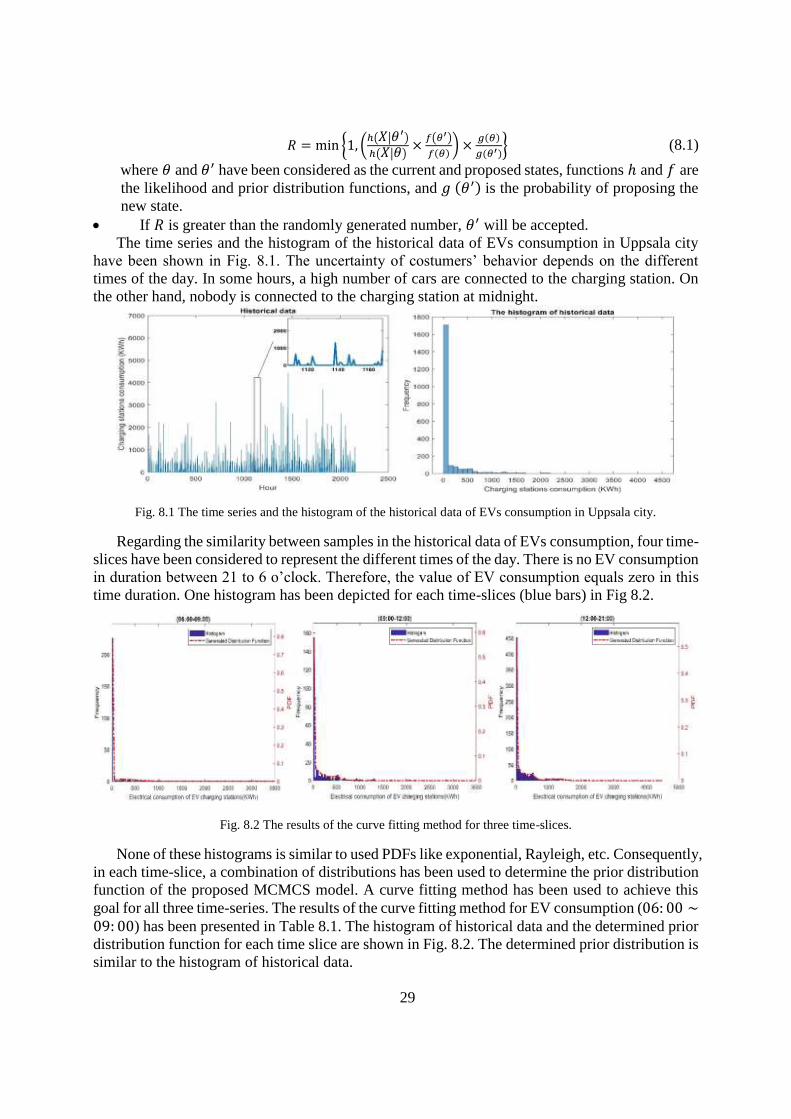
The time series and the histogram of the historical data of EVs consumption in Uppsala city

have been shown in Fig. 8.1. The uncertainty of costumers’ behavior depends on the different

times of the day. In some hours, a high number of cars are connected to the charging station. On

the other hand, nobody is connected to the charging station at midnight.

Fig. 8.1 The time series and the histogram of the historical data of EVs consumption in Uppsala city.

Regarding the similarity between samples in the historical data of EVs consumption, four time-

slices have been considered to represent the different times of the day. There is no EV consumption

in duration between 21 to 6 o’clock. Therefore, the value of EV consumption equals zero in this

time duration. One histogram has been depicted for each time-slices (blue bars) in Fig 8.2.

Fig. 8.2 The results of the curve fitting method for three time-slices.

None of these histograms is similar to used PDFs like exponential, Rayleigh, etc. Consequently,

in each time-slice, a combination of distributions has been used to determine the prior distribution

function of the proposed MCMCS model. A curve fitting method has been used to achieve this

goal for all three time-series. The results of the curve fitting method for EV consumption (06: 00 ∼09: 00) has been presented in Table 8.1. The histogram of historical data and the determined prior

distribution function for each time slice are shown in Fig. 8.2. The determined prior distribution is

similar to the histogram of historical data.

30

The variation of the EVs consumption in the historical data has been divided into ten sections

to determine the likelihood function. Each section has been taken into account as one state of the

MCMCS model. Consequently, the likelihood of moving from one state to another is determined.

In each iteration of the MCMCS model, one uniformly distributed number is generated.

Regarding the generated value and the corresponding time-slice, to make time-series, one row of

the table is chosen. Then, based on the PDF of the selected row, one random value is produced.

Then, the likelihood of moving from a previous state to a new one is calculated. Finally, the

decision about the acceptance of a new sample is made. This process is continued until the last

iteration of the MCMCS model.

Table 8.1 The Result of the Curve Fitting Method for EV Consumption (06: 00 ∼ 09: 00).

Uniform distribution Selected distribution

function

Coefficient A

(Shape)

Coefficient B

(Scale)

EV consumption(kWh)

Min Max Min Max

0 0,76 Beta 0,005 35,88 0 1500

0,76 0,8 Beta 0,2 15,79 0 3500

0,8 0,97 Beta 2 5,8 0 1500

0,97 1 Uniform - - 1000 3500

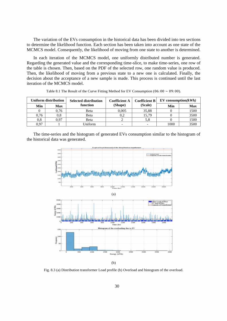
The time-series and the histogram of generated EVs consumption similar to the histogram of

the historical data was generated.

(a)

(b)

Fig. 8.3 (a) Distribution transformer Load profile (b) Overload and histogram of the overload.

31

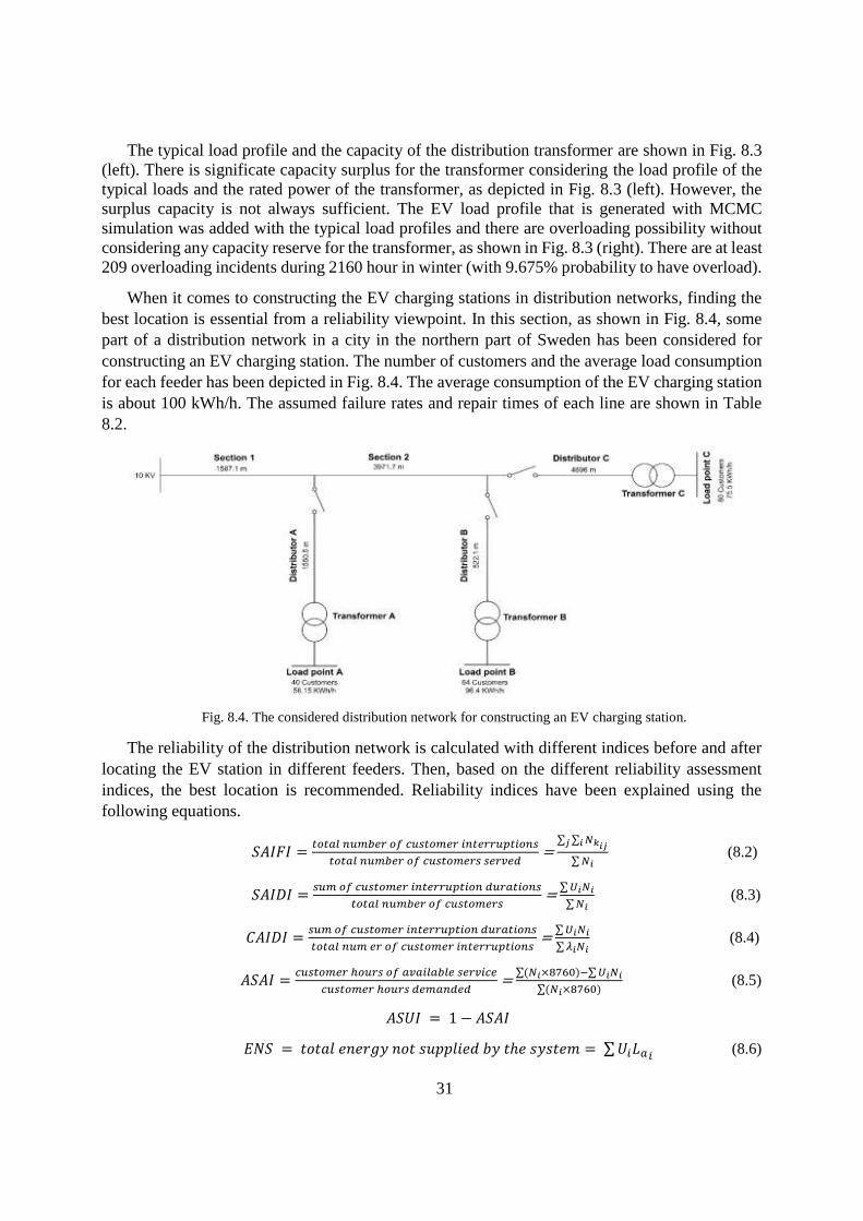
The typical load profile and the capacity of the distribution transformer are shown in Fig. 8.3

(left). There is significate capacity surplus for the transformer considering the load profile of the

typical loads and the rated power of the transformer, as depicted in Fig. 8.3 (left). However, the

surplus capacity is not always sufficient. The EV load profile that is generated with MCMC

simulation was added with the typical load profiles and there are overloading possibility without

considering any capacity reserve for the transformer, as shown in Fig. 8.3 (right). There are at least

209 overloading incidents during 2160 hour in winter (with 9.675% probability to have overload).

When it comes to constructing the EV charging stations in distribution networks, finding the

best location is essential from a reliability viewpoint. In this section, as shown in Fig. 8.4, some

part of a distribution network in a city in the northern part of Sweden has been considered for

constructing an EV charging station. The number of customers and the average load consumption

for each feeder has been depicted in Fig. 8.4. The average consumption of the EV charging station

is about 100 kWh/h. The assumed failure rates and repair times of each line are shown in Table

8.2.

Fig. 8.4. The considered distribution network for constructing an EV charging station.

The reliability of the distribution network is calculated with different indices before and after

locating the EV station in different feeders. Then, based on the different reliability assessment

indices, the best location is recommended. Reliability indices have been explained using the

following equations.

𝑆𝐴𝐼𝐹𝐼 =𝑡𝑜𝑡𝑎𝑙 𝑛𝑢𝑚𝑏𝑒𝑟 𝑜𝑓 𝑐𝑢𝑠𝑡𝑜𝑚𝑒𝑟 𝑖𝑛𝑡𝑒𝑟𝑟𝑢𝑝𝑡𝑖𝑜𝑛𝑠

𝑡𝑜𝑡𝑎𝑙 𝑛𝑢𝑚𝑏𝑒𝑟 𝑜𝑓 𝑐𝑢𝑠𝑡𝑜𝑚𝑒𝑟𝑠 𝑠𝑒𝑟𝑣𝑒𝑑 =

∑ ∑ 𝑁𝑘𝑖𝑗𝑖𝑗

∑ 𝑁𝑖 (8.2)

𝑆𝐴𝐼𝐷𝐼 =𝑠𝑢𝑚 𝑜𝑓 𝑐𝑢𝑠𝑡𝑜𝑚𝑒𝑟 𝑖𝑛𝑡𝑒𝑟𝑟𝑢𝑝𝑡𝑖𝑜𝑛 𝑑𝑢𝑟𝑎𝑡𝑖𝑜𝑛𝑠

𝑡𝑜𝑡𝑎𝑙 𝑛𝑢𝑚𝑏𝑒𝑟 𝑜𝑓 𝑐𝑢𝑠𝑡𝑜𝑚𝑒𝑟𝑠 =

∑ 𝑈𝑖𝑁𝑖

∑ 𝑁𝑖 (8.3)

𝐶𝐴𝐼𝐷𝐼 =𝑠𝑢𝑚 𝑜𝑓 𝑐𝑢𝑠𝑡𝑜𝑚𝑒𝑟 𝑖𝑛𝑡𝑒𝑟𝑟𝑢𝑝𝑡𝑖𝑜𝑛 𝑑𝑢𝑟𝑎𝑡𝑖𝑜𝑛𝑠

𝑡𝑜𝑡𝑎𝑙 𝑛𝑢𝑚 𝑒𝑟 𝑜𝑓 𝑐𝑢𝑠𝑡𝑜𝑚𝑒𝑟 𝑖𝑛𝑡𝑒𝑟𝑟𝑢𝑝𝑡𝑖𝑜𝑛𝑠 =

∑ 𝑈𝑖𝑁𝑖

∑ 𝜆𝑖𝑁𝑖 (8.4)

𝐴𝑆𝐴𝐼 =𝑐𝑢𝑠𝑡𝑜𝑚𝑒𝑟 ℎ𝑜𝑢𝑟𝑠 𝑜𝑓 𝑎𝑣𝑎𝑖𝑙𝑎𝑏𝑙𝑒 𝑠𝑒𝑟𝑣𝑖𝑐𝑒

𝑐𝑢𝑠𝑡𝑜𝑚𝑒𝑟 ℎ𝑜𝑢𝑟𝑠 𝑑𝑒𝑚𝑎𝑛𝑑𝑒𝑑 =

∑(𝑁𝑖×8760)−∑ 𝑈𝑖𝑁𝑖

∑(𝑁𝑖×8760) (8.5)

𝐴𝑆𝑈𝐼 = 1 − 𝐴𝑆𝐴𝐼

𝐸𝑁𝑆 = 𝑡𝑜𝑡𝑎𝑙 𝑒𝑛𝑒𝑟𝑔𝑦 𝑛𝑜𝑡 𝑠𝑢𝑝𝑝𝑙𝑖𝑒𝑑 𝑏𝑦 𝑡ℎ𝑒 𝑠𝑦𝑠𝑡𝑒𝑚 = ∑ 𝑈𝑖𝐿𝑎𝑖 (8.6)

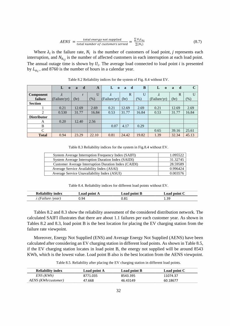
32

𝐴𝐸𝑁𝑆 =𝑡𝑜𝑡𝑎𝑙 𝑒𝑛𝑒𝑟𝑔𝑦 𝑛𝑜𝑡 𝑠𝑢𝑝𝑝𝑙𝑖𝑒𝑑

𝑡𝑜𝑡𝑎𝑙 𝑛𝑢𝑚𝑏𝑒𝑟 𝑜𝑓 𝑐𝑢𝑠𝑡𝑜𝑚𝑒𝑟𝑠 𝑠𝑒𝑟𝑣𝑒𝑑=

∑ 𝑈𝑖𝐿𝑎𝑖

∑(𝑁𝑖) (8.7)

Where 𝜆𝑖 is the failure rate, 𝑁𝑖 is the number of customers of load point, 𝑗 represents each

interruption, and 𝑁𝑘𝑖𝑗 is the number of affected customers in each interruption at each load point.

The annual outage time is shown by 𝑈𝑖. The average load connected to load point 𝑖 is presented

by 𝐿𝑎𝑖 , and 8760 is the number of hours in a calendar year.

Table 8.2 Reliability indices for the system of Fig. 8.4 without EV.

L o a d A

L o a d B

L o a d C

Component

failure

𝜆

(Failure/yr)

r

(hr)

U

(%) 𝜆

(Failure/yr)

R

(hr)

U

(%) 𝜆

(Failure/yr)

R

(hr)

U

(%)

Section

1 0.21 12.69 2.69 0.21 12.69 2.69 0.21 12.69 2.69

2 0.530 31.77 16.84 0.53 31.77 16.84 0.53 31.77 16.84

Distributor

A 0.20 12.40 2.56

B 0.07 4.17 0.29

C 0.65 39.16 25.61

Total 0.94 23.29 22.10 0.81 24.42 19.82 1.39 32.34 45.13

Table 8.3 Reliability indices for the system in Fig.8.4 without EV.

System Average Interruption Frequency Index (SAIFI) 1.095522

System Average Interruption Duration Index (SAIDI) 31.32745

Customer Average Interruption Duration Index (CAIDI) 28.59589

Average Service Availability Index (ASAI) 0.996424

Average Service Unavailability Index (ASUI) 0.003576

Table 8.4. Reliability indices for different load points without EV.

Reliability index Load point A Load point B Load point C

λ (Failure /year) 0.94 0.81 1.39

Tables 8.2 and 8.3 show the reliability assessment of the considered distribution network. The

calculated SAIFI illustrates that there are about 1.1 failures per each customer year. As shown in

Tables 8.2 and 8.3, load point B is the best location for placing the EV charging station from the

failure rate viewpoint.

Moreover, Energy Not Supplied (ENS) and Average Energy Not Supplied (AENS) have been

calculated after considering an EV charging station in different load points. As shown in Table 8.5,

if the EV charging station locates in load point B, the energy not supplied will be around 8543

KWh, which is the lowest value. Load point B also is the best location from the AENS viewpoint.

Table 8.5. Reliability after placing the EV charging station in different load points.

Reliability index Load point A Load point B Load point C

ENS (KWh) 8771.035 8543.395 11074.37

AENS (KWh/customer) 47.668 46.43149 60.18677

33

9. CURTAILMENT DEMAND ESTIMATION UNDER LARGE CHARGING LOAD

Consumption data for 15 Swedish cities for a period of 12.5 years (January 2008 to 2020 August)

are used to estimate the peak load of each city. The template of the non-hourly-read consumption,

as published at mimer.svk.se, has been used to estimate the consumption of the cities. This is

admittedly an underestimation, but still a good reference to compare with expected future demand

from EV charging. To obtain the future additional load due to large charging installations the

statistics of vehicle such as cars, buses and lorries are obtained from the Swedish statistical

database [65]. The expected charging power was calculated based on the number of vehicles,

charging power of the vehicle in kWh/km and covering range in km/hr. In the case of battery

operated electric buses and lorries it is considered that when 50 % of vehicles are charging the

remaining 50 % is on fleet. Analyst can easily predict that expected car charging load is more as

compared to the battery-electric busses and battery electric lorries. Fig. 9.1 represent that

additional charging load (yellow bar) for Stockholm, Uppsala, Jönköping and other cities are

greater than the peak load.

Fig. 9.1 Expected charging load for 15 cities in Sweden.

If the total load is greater than the rated value then overloading situation will occur. In general the

hosting capacity (HC) is defined as the amount of load that can be added without endangering the

reliability of the grid [66]. But here HC is computed in terms of needed curtailment hr/yr when the

additional charging load is added. From Table 9.1 it can be easily observed that as the HC in terms

of curtailment (hr/yr) is increased more number of cars and busses can be added.

Nonetheless, there is a social and economic limit to perform curtailment. From Fig. 9.2 it can be

inferred that as the additional charging load percentage is increased, the risk of curtailment would

also increase.

For instance from Fig. 9.2, for Stockholm if the load is 8.33% then the required curtailment would

be 9.923 approximately 10 hr/year. As the load is increased from 8.33% to 11.29 %, the need for

curtailment also increases and the grid operator has to perform curtailment during 20 hr/yr.

0

100

200

300

400

500

600

700

800

Char

gin

g l

oad

In M

W

Passenger cars

Battery Electric Busses

Heavy lorries / Battery electric long haul truck

Additional load for each city

Peak Load during last 10 Years

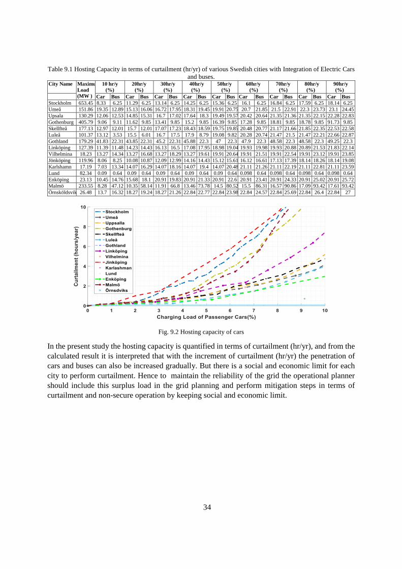
34

Table 9.1 Hosting Capacity in terms of curtailment (hr/yr) of various Swedish cities with Integration of Electric Cars

and buses. City Name Maximum

Load

(MW )

10 hr/y

(%)

20hr/y

(%)

30hr/y

(%)

40hr/y

(%)

50hr/y

(%)

60hr/y

(%)

70hr/y

(%)

80hr/y

(%)

90hr/y

(%)

Car Bus Car Bus Car Bus Car Bus Car Bus Car Bus Car Bus Car Bus Car Bus

Stockholm 653.45 8.33 6.25 11.29 6.25 13.14 6.25 14.25 6.25 15.36 6.25 16.1 6.25 16.84 6.25 17.59 6.25 18.14 6.25

Umeå 151.86 19.35 12.89 15.13 16.06 16.72 17.95 18.31 19.45 19.91 20.75 20.7 21.85 21.5 22.91 22.3 23.73 23.1 24.45

Upsala 130.29 12.06 12.53 14.85 15.31 16.7 17.02 17.64 18.3 19.49 19.57 20.42 20.64 21.35 21.36 21.35 22.15 22.28 22.83

Gothenburg 405.79 9.06 9.11 11.62 9.85 13.41 9.85 15.2 9.85 16.39 9.85 17.28 9.85 18.81 9.85 18.78 9.85 91.73 9.85

Skellfteå 177.13 12.97 12.01 15.7 12.01 17.07 17.23 18.43 18.59 19.75 19.85 20.48 20.77 21.17 21.66 21.85 22.35 22.53 22.58

Luleå 101.37 13.12 3.53 15.5 6.01 16.7 17.5 17.9 8.79 19.08 9.82 20.28 20.74 21.47 21.5 21.47 22.21 22.66 22.87

Gothland 179.29 41.83 22.31 43.85 22.31 45.2 22.31 45.88 22.3 47 22.3 47.9 22.3 48.58 22.3 48.58 22.3 49.25 22.3

Linköping 127.39 11.39 11.48 14.23 14.43 16.13 16.5 17.08 17.95 18.98 19.04 19.93 19.98 19.93 20.88 20.89 21.53 21.83 22.14

Vilhelmina 18.23 13.27 14.34 13.27 16.68 13.27 18.29 13.27 19.61 19.91 20.64 19.91 21.51 19.91 22.54 19.91 23.12 19.91 23.85

Jönköping 119.96 8.06 8.25 10.08 10.87 12.09 12.99 14.16 14.43 15.12 15.61 16.12 16.61 17.13 17.39 18.14 18.26 18.14 19.08

Karlshamn 17.19 7.03 13.34 14.07 16.29 14.07 18.16 14.07 19.4 14.07 20.48 21.11 21.26 21.11 22.19 21.11 22.81 21.11 23.59

Lund 82.34 0.09 0.64 0.09 0.64 0.09 0.64 0.09 0.64 0.09 0.64 0.098 0.64 0.098 0.64 0.098 0.64 0.098 0.64

Enköping 23.13 10.45 14.76 15.68 18.1 20.91 19.83 20.91 21.33 20.91 22.6 20.91 23.41 20.91 24.33 20.91 25.02 20.91 25.72

Malmö 233.55 8.28 47.12 10.35 58.14 11.91 66.8 13.46 73.78 14.5 80.52 15.5 86.31 16.57 90.86 17.09 93.42 17.61 93.42

Örnsköldsvik 26.48 13.7 16.32 18.27 19.24 18.27 21.26 22.84 22.77 22.84 23.98 22.84 24.57 22.84 25.69 22.84 26.4 22.84 27

Fig. 9.2 Hosting capacity of cars

In the present study the hosting capacity is quantified in terms of curtailment (hr/yr), and from the

calculated result it is interpreted that with the increment of curtailment (hr/yr) the penetration of

cars and buses can also be increased gradually. But there is a social and economic limit for each

city to perform curtailment. Hence to maintain the reliability of the grid the operational planner

should include this surplus load in the grid planning and perform mitigation steps in terms of

curtailment and non-secure operation by keeping social and economic limit.

35

10. IMPACT OF TEMPERATURE ON EV HOSTING CAPACITY

Driving conditions and ambient temperature are the factors that affect the energy requirement

of the battery and vehicle. The regional difference in energy consumption pattern of these BEVs

enforce a risk to the operators if proper planning is not done. In Europe, ambient temperatures

between −30 ºC to +40 ºC are observed and their impacts on the EV batteries cannot be neglected.

The annual energy consumption due to electric vehicle in northern Sweden during winter will be

higher compared to southern Sweden due to the temperature difference between the regions. On

the other hand, Sweden is looking forward for 100% renewable electricity generation by 2040.

Thus with the drastic growth of EV’s the northern Sweden during colder months need to rely on

wind and hydro power since the solar production will be very low during colder months.

During cold weather conditions, the EV’s battery efficiency decreases and the battery internal

resistance increases affecting the discharge capability of battery. In addition more energy is

required for cabin air conditioning. More energy is also needed at high temperature. Nissan leaf

users data analysis on Electric Range in Cold Weather report upto 40% decline in driving range

on a cold / hot weather. Subsequently, reduced vehicle efficiency results in increased energy

consumption and increased need for charging from the electric grid.

The hosting-capacity is a proven measure to quantify the ability of the grid to accept EV

charging. A lot of research on hosting capacity of EV integration with the grid had been carried

out [67],[68],[69],[70]. Such research mainly focused on developing models based on coordinated

charging strategy, stochastic approach for uncoordinated EV charging [67], travel behaviour, state

of charge (SOC) and charging level type [68], robust optimization model with adjustable

uncertainty, model based on synergies between EV charging and PV power production to reduce

peak loads [69], etc. In [70] a probabilistic mathematical model of Electric Vehicle charging

demand was established. The hosting capacity of EV was evaluated using cumulants and Gram-

Charlies series expansion for an IEEE 33 node distribution network. The impact of ambient

temperature is however not included in such studies. The main objective of this work is to estimate

the hosting capacity of a MV/ LV grid considering ambient temperature variation during the EVs

fleet and charging. For this purpose, an existing 130/10 kV distribution grid in northern Sweden

consisting of two 30 MVA transformers (T3a and T3b) separated by a sectioning switch is

investigated. The station has three main 10 kV outgoing feeders and 6-MV/LV, 800 kVA

transformers. The 10 kV distribution network has a total length of 2774.9 metres and is connected

to a total of 588-customers in the low-voltage network.

Fig. 10.1(left) shows the combined T3a and T3b one year load data in kA acquired in 10 minute

interval on the 10 kV side of 30 MVA transformers, without EV integration. The temperature

variation of the region of the transformer during the period of study is given in Fig. 10.1(right).

The hosting capacity of a transformer, for new consumption like EV charging, is the difference

between the transformer rating and the loading without EV charging. To include the impact of the

ambient temperature variation on the charging demand a correction factor 𝐾𝑇 has been introduced

in the hosting capacity equation. This correction factor quantifies how much more electricity the

car needs because of ambient temperature not being equal to 20ºC.

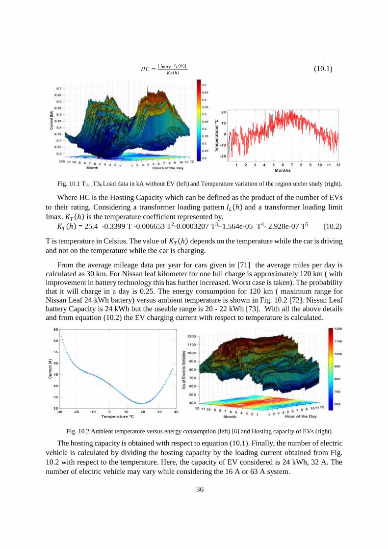
36

𝐻𝐶 = [ 𝐼𝑚𝑎𝑥−𝐼𝐿(ℎ)]

𝐾𝑇(ℎ) (10.1)

Fig. 10.1 T3a ,T3b Load data in kA without EV (left) and Temperature variation of the region under study (right).

Where HC is the Hosting Capacity which can be defined as the product of the number of EVs

to their rating. Considering a transformer loading pattern 𝐼𝐿(ℎ) and a transformer loading limit

Imax. 𝐾𝑇(ℎ) is the temperature coefficient represented by,

𝐾𝑇(ℎ) = 25.4 -0.3399 T -0.006653 T2-0.0003207 T3+1.564e-05 T4- 2.928e-07 T5 (10.2)

T is temperature in Celsius. The value of 𝐾𝑇(ℎ) depends on the temperature while the car is driving

and not on the temperature while the car is charging.

From the average mileage data per year for cars given in [71] the average miles per day is

calculated as 30 km. For Nissan leaf kilometer for one full charge is approximately 120 km ( with

improvement in battery technology this has further increased. Worst case is taken). The probability

that it will charge in a day is 0.25. The energy consumption for 120 km ( maximum range for

Nissan Leaf 24 kWh battery) versus ambient temperature is shown in Fig. 10.2 [72]. Nissan Leaf

battery Capacity is 24 kWh but the useable range is 20 - 22 kWh [73]. With all the above details

and from equation (10.2) the EV charging current with respect to temperature is calculated.

Fig. 10.2 Ambient temperature versus energy consumption (left) [6] and Hosting capacity of EVs (right).

The hosting capacity is obtained with respect to equation (10.1). Finally, the number of electric

vehicle is calculated by dividing the hosting capacity by the loading current obtained from Fig.

10.2 with respect to the temperature. Here, the capacity of EV considered is 24 kWh, 32 A. The

number of electric vehicle may vary while considering the 16 A or 63 A system.

37

For 30 MVA transformer in Fig. 10.2 (right) it is observed that the hosting capacity during the hot

months June and July is higher compared to the colder months of December and January. The

hosting capacity of EVs with and without temperature coefficient 𝐾𝑇(ℎ) is shown in Fig. 10.3.

Fig. 10.3 Hosting capacity of EVs with and without temperature coefficient (left) and % change in hosting capacity

(right).

By introducing the temperature coefficient 𝐾𝑇(ℎ) there is around 30% decrease in hosting

capacity during colder months due to fast discharge of battery as shown in Fig. 10.3. Henceforth,

this study helps the network operators to plan the EV charging strategies based on the climate and

the region.

38

11. CONCLUSION

The purpose of this study was to develop a synthesis of knowledge of the impact that

electromobility can have on the power grid and to map the knowledge gaps. Several aspects in

service and power quality at the MV and LV networks were investigated from the point of view

of TSO, DSO, utilities and customers. From this, the impacts and challenges were summarized in

different sections.

The presence of waveform distortions such as harmonics, interharmonics and supraharmonics

are reported during EV charging and are verified using measurements. An attempt was made to

determine how they aggregate and propagate in a low and medium voltage network with multiple

EV integration. Initially the PDF of the dominant lower order harmonics were studied. It was found

different for different charging cycle because of different uncertainties such as battery SOC,

background distortion level, charging rate, power electronic technology used etc. Hence there is a

need to develop a new method to address this issue. The interharmonics aggregation study

concluded that the aggregation peak current value depends on the randomness of the number of

EVs charging. With a random number of EVs connected to the grid the distribution is an extreme

value distribution and it loses its skewness and become normal for constant number of EVs. Hence

in reality with random number of EVs the standard summation rule fails. In the supraharmonics

range the necessity of unified measurements, immunity/standardization and interference

knowledge for aggregation studies are emphasized. Though the magnitude of supraharmonics

current is very low, they get superimposed on primary and secondary emissions while they

propagate through protective earth (PE) and cause unnecessary tripping of RCD. It was also

inferred that the EVs connected to installations with TN-C-S earthing of high capacitance and low

resistance will experience high leakage current.

EV chargers are not affected by shallow voltage dips. While considering the Swedish network

with underground cables in transmission and distribution, even a fault with shallow dip cause large

transient at the beginning of the dip due to the switching of cable capacitance. When this dip get

propagated to the distribution grid it may get amplified (high impedance grid) based on the

resonant frequency. Hence, even a shallow dip with a phase angle jump (PAJ) of 20oC has a big

impact on the EV charging and the life of the battery. EV while discharging are more sensitive to

asymmetric dips with phase angle jump as they cause high overvoltage and oscillations at the dc

link of the EV charger. This impact is noticeable while less number of EVs are charging.

The light flicker due to fast voltage variation caused by EVs charging mainly depends on the

number of EVs connected, the topology of the LED lamps used by the customers and the

impedance of the grid. Though the flicker is more prominent in a weaker grid (high grid

impedance) it mainly depends more on the lamp topology. The lamps with active power factor

correction (examined based on the current waveform) is more sensitive to fast voltage variation

and cause light flicker.

PV-EV hosting capacity was determined using a stochastic approach considering the

undervoltage phenomenon. The investigation concluded that the impact of electric vehicle

charging during day time is lesser than the impact during the night time and it also depends on the

relative coincidence factor between PV and EV. The likelihood for an undervoltage for single-

39

phase and three-phase is very small during day time and is high during the night time. The

likelihood of an undervoltage violation increases with the increase in charging power and

penetration level.

The hosting capacity study quantified in terms of curtailment (hr/yr), determines that the

penetration of large rated electric vehicles can be increased gradually with the increment of

curtailment (hr/yr) keeping in view the social and economic limit. Considering overloading

conditions taking into account the load profile of northern Sweden the hosting capacity is

quantified surplus, but with certain risk during winters. The study also calculates the reliability

index to determine the optimal location for the EV integration with respect to the Average Energy

Not Supplied (AENS) index value. A similar study investigated the hosting capacity using

probabilistic dynamic line rating (DLR) for northern Sweden during the period 2011 and 2018. Its

shows that by using DLR the minimum capacity will increase up to 56% of the maximum transfer

capacity with static rating during the peak load period in winter. Since real-time study is based

on perfect knowledge of the environmental parameters it is important to take in to account the

uncertainty in the DLR calculation using probabilistic approach. Probabilistic DLR, where the

probability of overload is used as a decision criterion, can provide more hosting capacity in terms

of number of EV cars. It will allow a continuous, hour-by-hour, trade-off between accepting some

certain level of risks or neglecting them. A study on the impact of temperature on the EV hosting

capacity inferred that by introducing the temperature coefficient there is around 30% decrease in

hosting capacity during colder months due to fast discharge of batteries. Hence to maintain the

reliability of the grid the operational planner should include this surplus load and risks in the grid

along with the temperature factor inferred from the above studies while planning and perform

mitigation steps in terms of curtailment and non-secure operation keeping in view the social and

economic limit.

Results from the project can be expected to be used by other researchers as a basis for deeper

studies, by electricity network companies as a basis for strengthening or otherwise adapting their

electricity networks, by manufacturers and charging infrastructure to reduce interference emissions

and improve interference resistance, and to define future guidelines, connection requirements and

standards. Results can also be used as input for the design of "smart charging" and the design of

electricity markets.

The project will also lead to increased knowledge about how new appliances affect the electricity

grid and how the electricity grid will affect new appliances. This knowledge will also be useful

when connecting other new types of devices, such as photovoltaic systems, battery storage, new

types of lighting, energy-efficient devices, etc.

40

12. REFERENCES

[1] L. Kutt, E. Saarijarvi, M. Lehtonen, H. Molder, and J. Niitsoo, “A review of the harmonic

and unbalance effects in electrical distribution networks due to EV charging,” in 12th

International Conference on Environment and Electrical Engineering, EEEIC 2013,

Wroclaw, pp. 556–561, 2013. doi: 10.1109/EEEIC.2013.6549577.

[2] A. Lucas, F. Bonavitacola, E. Kotsakis, and G. Fulli, “Grid harmonic impact of multiple

electric vehicle fast charging,” Electr. Power Syst. Res., vol. 127, pp. 13–21, Jun. 2015. doi:

10.1016/j.epsr.2015.05.012.

[3] A. J. Collin, Xiao Xu, S. Z. Djokic, F. Möller, J. Meyer, L. Kutt, M. Lehtonen, “Survey of

harmonic emission of electrical vehicle chargers in the European market,” in 2016

International Symposium on Power Electronics, Electrical Drives, Automation and Motion,

SPEEDAM 2016, Jul. 2016, pp. 1208–1213, doi: 10.1109/SPEEDAM.2016.7526005.

[4] X. Nie et al., "Online monitoring and integrated analysis system for EV charging

station," 2013 IEEE PES Asia-Pacific Power and Energy Engineering Conference

(APPEEC), Kowloon, 2013, pp. 1-6.

[5] Z. Jin, H. Zhang, F. Shi, Y. Sun and V. Terzija, "A Robust and Adaptive Detection Scheme

for Interharmonics in Active Distribution Network," in IEEE Transactions on Power

Delivery, vol. 33, no. 5, pp. 2524-2534, Oct. 2018

[6] V. Ravindran, S. L. Shimi, S. K. Rönnberg, and M. H. J. Bollen, “Time domain aggregation

of interharmonics from power converters of sustainable sources,” Communicated.

[7] R. Torquato, G. R. T. Hax, W. Freitas, and S. Member, “Impact Assessment of High-

Frequency Distortions Produced by PV Inverters,” in IEEE Transactions on Power Delivery,

pp 1–9, 2020. doi: 10.1109/TPWRD.2020.3031375.

[8] T. M. H. Slangen, T. van Wijk, V. Ćuk and J. F. G. Cobben, "The Harmonic and

Supraharmonic Emission of Battery Electric Vehicles in The Netherlands," 2020

International Conference on Smart Energy Systems and Technologies (SEST), Istanbul,

Turkey, 2020, pp. 1-6, doi: 10.1109/SEST48500.2020.9203533.

[9] D. Darmawardana et al., "Investigation of high frequency emissions (supraharmonics) from

small, grid-tied, photovoltaic inverters of different topologies," 18th International

Conference on Harmonics and Quality of Power (ICHQP), Ljubljana, 2018, pp. 1-6, doi:

10.1109/ICHQP.2018.8378926.

[10] J. Meyer, S. Haehle and P. Schegner, "Impact of higher frequency emission above 2kHz on

electronic mass-market equipment," 22nd International Conference and Exhibition on

Electricity Distribution (CIRED 2013), Stockholm, 2013, pp. 1-4, doi:

10.1049/cp.2013.1027.

[11] S. Selcuk, S. Rönnberg, and M. Bollen, "Interferences in AC–DC LED Drivers Exposed to

Voltage Disturbances in the Frequency Range 2–150 kHz, " IEEE Transactions on Power

Electronics, Vol.34, Issue 11, 11171-11181, 2019.

[12] J. Yaghoobi, A. Alduraibi, D. Martin, F. Zare, and D. Eghbal, “Electrical Power and Energy

Systems Impact of high-frequency harmonics ( 0 – 9 kHz ) generated by grid-connected

inverters on distribution transformers,” Electr. Power Energy Syst., vol. 122, no. April, p.

106177, 2020.

[13] T. M. H. Slangen, T. van Wijk, V. Ćuk and J. F. G. Cobben, “The Propagation and

Interaction of Supraharmonics from Electric Vehicle Chargers in a Low-Voltage Grid,”

Energies , Vol. 13, Issue 15, pp. 3865,2020. https://doi.org/10.3390/en13153865.

[14] T. Wohlfahrt, C. Waniek, and J. M. A. Myrzik, “Optimization Measures for Increased

41

Immunity against High Frequency Disturbances and Reduced Emission in the Range of 2

kHz to 150 kHz Realized on Different LED Lamps Key words,” Renewable Energy and

Power Quality Journal, vol. 1, no. 15, pp. 251–254, 2017.

[15] A. Espín-Delgado, S.S Letha, S. K. Ronnberg, M. H. J. Bollen , “Failure of MV Cable

Terminations Due to Supraharmonic Voltages : A Risk Indicator,” IEEE Open Journal of

Industry Applications, vol. 1, no. April, 2020.

[16] V. Khokhlov, J. A. N. Meyer, and S. Member, “Comparison of Measurement Methods for

the Frequency Range 2-150 kHz ( Supraharmonics ) Based on the Present Standards

Framework,” Special Section on Addressing Challenging Issues of Grids with High

Penetration, IEEE Access, vol. 8, 2020.

[17] Z. Wang, X. Guo, J. Li and X. Wang, "Impact of Voltage Sags on Electric-Vehicle Charger

and Critical Voltage Sag Determination," in IEEE Transactions on Power Delivery, vol. 31,

no. 3, pp. 1397-1399, June 2016, doi: 10.1109/TPWRD.2015.2473100.

[18] Society of Automotive Engineers Standard J2894–1, "Power Quality Requirements for Plug-

In Electric Vehicle Chargers, ", Dec. 2011.

[19] S. Kundu and I. A. Hiskens, "Overvoltages due to synchronous tripping of plug-in electric-

vehicle chargers following voltage dips," IEEE Transaction on Power Delivery, vol. 29, no.

3, pp. 1147-1156, June 2014.

[20] S. Hui and X. Yonghai, "Study on the impact of voltage sags on different types of electric

vehicle chargers," 2016 China International Conference on Electricity Distribution

(CICED), Xi'an, 2016, pp. 1-4, doi: 10.1109/CICED.2016.7576319.

[21] M. H. J. Bollen, "On voltage dip propagation," 2001 Power Engineering Society Summer

Meeting. Conference Proceedings (Cat. No.01CH37262), Vancouver, BC, Canada, 2001, pp.

665-670 vol.1, doi: 10.1109/PESS.2001.970121.

[22] U. Johansson och U. Grape "Förberedande kartläggning av spänningsdippar i olika typer av

nät. " Elforsk rapport 04:43, 2004.

[23] L. Oscar, and M. H. J. Bollen. "Impact of uncertainties on resonant overvoltages."

International Conference on Power Systems Transients (IPST), 2019.

[24] O. Tremblay, L. Dessaint and A. Dekkiche, "A Generic Battery Model for the Dynamic

Simulation of Hybrid Electric Vehicles," 2007 IEEE Vehicle Power and Propulsion

Conference, Arlington, TX, 2007, pp. 284-289, doi: 10.1109/VPPC.2007.4544139.

[25] H. Seljeseth, H. Taxt and T. Solvang, "Measurements of network impact from electric

vehicles during slow and fast charging," 22nd International Conference and Exhibition on

Electricity Distribution (CIRED 2013), Stockholm, 2013, pp. 1-4, doi:

10.1049/cp.2013.1197.

[26] IEEE Std 2030.1.1-2015, IEEE Standard Technical Specifications of a DC Quick Charger

for Use with Electric Vehicles, IEEE Vehicular Technology Society, 2015.

[27] Report on Impact of Electric Vehicle Charging on the power Grid, Electric Power Engineering

Group at Luleå University of Technology in Skellefteå, Sweden, December 2019.

[28] IEC 61000-3-7 Electromagnetic compatibility (EMC) – Part 3-7: Limits – Assessment of

emission limits for the connection of fluctuating installations to MV, HV and EHV power

systems, 2008.

[29] M. Lundmark, “High-Frequency Components in the Neutral and Protective Earth Currents

Due To Electronic Equipment,” in International Conference on Electricity Distribution:

21/05/2007-24/05/2007, 2007, no. 0370, pp. 21–24.

[30] A. M. Blanco, F. Moller, J. Meyer, and P. Schegner, “Characterization of the leakage

currents produced by household electronic devices,” Proc. Int. Conf. Harmon. Qual. Power,

42

ICHQP, vol. 2020-July, 2020, doi: 10.1109/ICHQP46026.2020.9177876.

[31] T. Slangen, T. van Wijk, V. Ćuk, and S. Cobben, “The propagation and interaction of

supraharmonics from electric vehicle chargers in a low-voltage grid,” Energies, vol. 13, no.

15, pp. 1–19, 2020, doi: 10.3390/en13153865.

[32] K. J. Brown, “Electric vehicle supply equipment; A safety device,” 2013 IEEE Transp.

Electrif. Conf. Expo Components, Syst. Power Electron. - From Technol. to Bus. Public

Policy, ITEC 2013, pp. 0–4, 2013, doi: 10.1109/ITEC.2013.6573505.

[33] H. Kirkeby, “Charging problems in EV-paradise,” in 25th International Conference on

Electricity Distribution, Madrid, Spain, June2019.

[34] J. Sutaria, A. Espin-Delgado, and S. Ronnberg, “Summation of Supraharmonics in Neutral

for Three-Phase Four-Wire System,” IEEE Open J. Ind. Appl., vol. 1, no. June, pp. 148–156,

2020, doi: 10.1109/ojia.2020.3026753.

[35] A. Grevener, J. Meyer, S. Rönnberg, M. Bollen, and J. Myrzik, “Survey of supraharmonic

emission of household appliances,” CIRED - Open Access Proc. J., vol. 2017, no. 1, pp.

870–874, 2017, doi: 10.1049/oap-cired.2017.0458.

[36] S. Rönnberg and A. Larsson, “A simple model for interaction between equipment at a

frequency od some tens of kHz,” in 21st International Conference on Electricity Distribution

Frankfurt, 2011, no. 0206, pp. 6–9.

[37] C. Rivers and T. F. Papallo, “Leakage current discrimination and masking from upstream

ground fault protection devices during electric vehicle charging,” 2012 IEEE Int. Electr. Veh.

Conf. IEVC 2012, pp. 2–7, 2012, doi: 10.1109/IEVC.2012.6183167.

[38] Á. Espín-delgado, S. Rönnberg, S.L Shimi, and M. Bollen, “Diagnosis of Supraharmonics-

related Problems Based on the Effects on Electrical Equipment,” Electr. Power Syst. Res.

(Communicated), pp. 1–22.

[39] E. Mulenga, M. H. J. Bollen, and N. Etherden, "Overvoltage due to single-phase and three-

phase connected PV and what to do about it," in Proc. of the 25th International Conference

on Electricity Distribution (CIRED 2019), Madrid, Spain, 2019, pp. 1-4.

[40] J. Dickert and P. Schegner, "Residential load models for network planning purposes," in

2010 Modern Electric Power Systems, 2010, pp. 1-6.

[41] Statista. (2020, 10 July). Share of elderly population in Sweden 1970-2019. Available:

https://www.statista.com/statistics/525637/sweden-elderly-share-of-the-total-population-

by-age-group/

[42] M. Muratori, "Impact of uncoordinated plug-in electric vehicle charging on residential power

demand," Nature Energy, vol. 3, pp. 193-201, Mar 2018.

[43] S. Su, H. Li, and D. W. Gao, "Optimal Planning of Charging for Plug-In Electric Vehicles

Focusing on Users’ Benefits," Energies, vol. 10, p. 952, 2017.

[44] Y. Wang and D. Infield, "Markov Chain Monte Carlo simulation of electric vehicle use for

network integration studies," International Journal of Electrical Power & Energy Systems,

vol. 99, pp. 85-94, 2018/07/01/ 2018.

[45] J. Vopava, U. Bergmann, and T. Kienberger, "Synergies between e-Mobility and

Photovoltaic Potentials—A Case Study on an Urban Medium Voltage Grid," Energies, vol.

13, p. 3795, 2020.

[46 ] G. Putrus, P. Suwanapingkarl, D. Johnston, E. Bentley, and M. Narayana, Impact of electric

vehicles on power distribution networks, IEEE Conference in Vehicle Power and Propulsion,

pp. 827–831, 2009.

43

[47] M. Coldwell, D. Strickland, and L. Chittock, “Impact of electric vehicles on GB electricity

demand and associated benefits for system control,” 48th International Universities’ in

Power Engineering Conference (UPEC), pp. 1–6, 2013.

[48] “IEEE Standard for Calculating the Current-Temperature Relationship of Bare Overhead

Conductors,” IEEE Std 738-2012, pp. 1–72, 2013.

[49] SF. Hajeforosh, and M. h.J. Bollen, Dynamic Line Rating Operational Planning: Issues and

Challenges, 25th International Conference and Exhibition on Electricity Distribution,

CIRED, 2019.

[50] S.F. Hajeforosh, and M. h.J. Bollen, Uncertainty Analysis of Stochastic Dynamic Line

Rating, Electric Power System Research, 2020.

[51] S.F. Hajeforosh, Math H.J. Bollen, Transmission Line Overloading Analysis Using

Probabilistic Dynamic Line Rating, International Conference on Probabilistic Methods

Applied to Power Systems (PMAPS), pp. 1-6, 2020.

[52] N. Hartmann and E. D. Özdemir, “Impact of different utilization scenarios of electric

vehicles on the German grid in 2030,” J. Power Sources, vol. 196, no. 4, pp. 2311–2318,

Feb. 2011, doi: 10.1016/j.jpowsour.2010.09.117.

[53] C. Weiller, “Plug-in hybrid electric vehicle impacts on hourly electricity demand in the

United States,” Energy Policy, vol. 39, no. 6, pp. 3766–3778, Jun. 2011, doi:

10.1016/j.enpol.2011.04.005.

[54] G. Razeghi, L. Zhang, T. Brown, and S. Samuelsen, “Impacts of plug-in hybrid electric

vehicles on a residential transformer using stochastic and empirical analysis,” J. Power

Sources, vol. 252, pp. 277–285, Apr. 2014, doi: 10.1016/j.jpowsour.2013.11.089.

[55] C. H. Dharmakeerthi, N. Mithulananthan, and T. K. Saha, “Overview of the impacts of plug-

in electric vehicles on the power grid,” 2011, doi: 10.1109/ISGT-Asia.2011.6167115.

[56] Q. Yan and M. Kezunovic, “Impact analysis of electric vehicle charging on distribution

system,” 2012, doi: 10.1109/NAPS.2012.6336413.

[57] C. Farkas, G. Szucs, and L. Prikler, “Grid impacts of twin EV fast charging stations placed

alongside a motorway,” 2013, doi: 10.1109/IYCE.2013.6604144.

[58] E. Akhavan-Rezai, M. F. Shaaban, E. F. El-Saadany, and A. Zidan, “Uncoordinated charging

impacts of electric vehicles on electric distribution grids: Normal and fast charging

comparison,” 2012, doi: 10.1109/PESGM.2012.6345583.

[59] J. R. Pillai and B. Bak-Jensen, “Impacts of electric vehicle loads on power distribution

systems,” 2010, doi: 10.1109/VPPC.2010.5729191.

[60] H. Wang, Q. Song, L. Zhang, F. Wen, and J. Huang, “Load characteristics of electric vehicles

in charging and discharging states and impacts on distribution systems,” in IET Conference

Publications, 2012, vol. 2012, no. 611 CP, doi: 10.1049/cp.2012.1837.

[61] C. Jiang, R. Torquato, D. Salles, and W. Xu, “Method to assess the power-quality impact of

plug-in electric vehicles,” IEEE Trans. Power Deliv., vol. 29, no. 2, pp. 958–965, 2014, doi:

10.1109/TPWRD.2013.2283598.

[62] M. Honarmand, A. Zakariazadeh, and S. Jadid, “Self-scheduling of electric vehicles in an

intelligent parking lot using stochastic optimization,” J. Franklin Inst., vol. 352, no. 2, pp.

449–467, Feb. 2015, doi: 10.1016/j.jfranklin.2014.01.019.

[63] M. Honarmand, A. Zakariazadeh, and S. Jadid, “Optimal scheduling of electric vehicles in

an intelligent parking lot considering vehicle-to-grid concept and battery condition,” Energy,

vol. 65, pp. 572–579, Feb. 2014, doi: 10.1016/j.energy.2013.11.045.

[64] D. van Ravenzwaaij, P. Cassey, and S. D. Brown, “A simple introduction to Markov Chain

Monte–Carlo sampling,” Psychon. Bull. Rev., vol. 25, no. 1, pp. 143–154, Feb. 2018, doi:

44

10.3758/s13423-016-1015-8

[65]https://www.statistikdatabasen.scb.se/pxweb/en/ssd/START__TK__TK1001__TK1001A/Fo

rdonTrafik/.

[66] M. Bollen and S. Rönnberg, "Hosting Capacity of the Power Grid for RenewableElectricity

Production and New LargeConsumption Equipment," Energies, vol. 10, no. 9, 2017.

[67] S. Cundeva , A.K Mateska, M. H. J. Bollen, Hosting capacity of LV residential grid for

uncoordinated EV charging, 18th International Conference on Harmonics and Quality of

Power, 2018. DOI: 10.1109/ICHQP.2018.8378892.

[68] S. Rout and GyanRanjan, "Hosting Capacity Assessment of Electric Vehicles Integration in

Active Distribution System," Biswal 2020, J. Phys.: Conf. Ser. 1478 012006, 2020.

[69] R. Fachrizal, J. Munkhammar, "Improved Photovoltaic Self-Consumption in Residential

Buildings with Distributed and Centralized Smart Charging of Electric Vehicles, " Energies,

202013, 1153; doi:10.3390/en13051153

[70] S. Wanga, C. Li , Z. Pan, J. Wang, "Probabilistic Method for Distribution Network Electric

Vehicle Hosting Capacity Assessment based on Combined Cumulants and Gram-Charlier

Expansion, " Energy Procedia, Vol.158, pp. 5067–5072, 2019.

[71] https://www.trafa.se/en/road-traffic/vehicle-statistics/

[72] T. Yuksel and J. J. Michalek, "Effects of Regional Temperature on Electric Vehicle Efficiency,

Range, and Emissions in the United States", Environmental Science and Technology, vol.

49, pp.3974−3980, 2015.

[73] https://ev-database.org/car/1019/Nissan-Leaf-24-kWh