IEEE TRANSACTIONS ON NEURAL NETWORKS, VOL. · PDF fileand sparse solution. ... (SMO) algorithm. ... 2009 at 00:02 from IEEE Xplore. Restrictions apply. 686 IEEE TRANSACTIONS ON NEURAL

IEEE TRANSACTIONS ON NEURAL NETWORKS, VOL. 18, NO. 3, MAY 2007 685

Fast Sparse Approximation for Least SquaresSupport Vector Machine

Licheng Jiao, Senior Member, IEEE, Liefeng Bo, and Ling Wang

Abstract—In this paper, we present two fast sparse approxima-tion schemes for least squares support vector machine (LS-SVM),named FSALS-SVM and PFSALS-SVM, to overcome the limita-tion of LS-SVM that it is not applicable to large data sets and toimprove test speed. FSALS-SVM iteratively builds the decisionfunction by adding one basis function from a kernel-based dic-tionary at one time. The process is terminated by using a flexibleand stable epsilon insensitive stopping criterion. A probabilisticspeedup scheme is employed to further improve the speed ofFSALS-SVM and the resulting classifier is named PFSALS-SVM.Our algorithms are of two compelling features: low complexityand sparse solution. Experiments on benchmark data sets showthat our algorithms obtain sparse classifiers at a rather low costwithout sacrificing the generalization performance.

Index Terms—Fast algorithm, greedy algorithm, least squaressupport vector machine (LS-SVM), sparse approximation.

I. INTRODUCTION

I N a classification problem, we are given a set of samples ofinput vectors along with corresponding class labels

, and the task is to find a deterministic function that bestrepresents the relation between input vectors and class labels.A successful method for classification problem is least squaressupport vector machine (LS-SVM) [1], [2], which attempts tominimize the least square error on the training samples whilesimultaneously maximizing the margin between two classes.

Extensive empirical comparisons [3] show that LS-SVM ob-tains good performance on various classification problems, buttwo obvious limitations still exist. First, the training procedureof LS-SVM amounts to solving a set of linear equations [4]. Al-though the training problem is, in principle, solvable, in practice,it is intractable for a large data set by the classical techniques,e.g., Gaussian elimination, because their computational com-plexity usually scales cubically with the size of training sam-ples. Second, the solution of LS-SVM lacks the sparseness and,hence, the test speed is significantly slower than other learningalgorithms such as support vector machine (SVM) [5], [6] andneural networks (NNs) [7], [8].

Many researchers have identified the aforementioned twolimitations and tried to give their solutions. As for the fast al-gorithms for LS-SVM, Suykens et al. [9] presented a conjugate

Manuscript received September 16, 2005; revised June 5, 2006; accepted Oc-tober 8, 2006. This work was supported by the National Natural Science Foun-dation of China under Grant 60372050 and the National Defense PreresearchFoundation of China under Grant A1420060172.

The authors are with the Institute of Intelligent Information Processing, Xi-dian University, Xi’an 710071, China (e-mail: [email protected]).

Digital Object Identifier 10.1109/TNN.2006.889500

gradient algorithm. Chu et al. [10] gave an improved conju-gate gradient algorithm. Keerthi and Shevade [11] proposed asequential minimal optimization (SMO) algorithm. Althoughthese algorithms achieve low complexity, their resulting solu-tions are not sparse. Hence, the second limitation still exists. Asfor the sparseness of LS-SVM, Suykens et al. [12], [13] pro-posed a simple approach to introduce the sparseness by sortingthe support value spectrum (SVS), i.e., the absolute value ofthe solution of LS-SVM. Kruif and Vries [14] presented a moresophisticated pruning mechanism that omits the sample bearingthe least error after it is omitted. Zeng and Chen [15] proposeda SMO-based pruning method. However, these algorithmsrequire solving a set of linear equations (slowly decreasingin size) many times, which incurs a large computational cost.Hence, the first limitation still exists. Furthermore, Suykenset al. [16] proposed fixed-size LS-SVM for fast finding thesparse approximate solution of LS-SVM. Unlike the algorithmsmentioned previously, fixed-size LS-SVM (FSLS-SVM) solvesthe least squares problem in the primal space instead of inthe dual space. Recently, Hoegaerts et al. [17] introduced thesimilar idea to solve kernel partial least squares regression.

In this paper, we present a fast sparse approximation schemefor LS-SVM (FSALS-SVM) to deal with the previous twolimitations simultaneously. FSALS-SVM iteratively buildsthe decision function by adding one basis function from akernel-based dictionary at one time until the -insensitive crite-rion is satisfied. FSALS-SVM consists of two key components:the selection of basis function and the solution of subproblem.By integrating some efficient schemes into these two compo-nents, FSALS-SVM is endowed with two compelling features:low complexity and sparse solution. It is possible to use aprobabilistic speedup scheme to further improve the speedof FSALS-SVM and the resulting classifier is named PF-SALS-SVM. Experiments on the benchmark data sets confirmthe feasibility and validity of FSALS-SVM and PFSALS-SVM.

The rest of the paper is organized as follows. In Section II,we briefly introduce LS-SVM. In Section III, we interpret whythe Wolfe dual of LS-SVM can be regarded as a regularizedloss function consisting of the loss function induced by repro-ducing Kernel–Hilbert space (RKHS) norm and of the regular-ization term. FSALS-SVM is proposed based on a backfittingscheme in Section IV. The convergence, probabilistic speedupand computational complexity of FSALS-SVM is detail-ana-lyzed in Section V. Related works are discussed in Section VI.Experimental results are reported in Section VII. Finally, inSection VIII, we give some concluding remarks.

For convenience, in Table I, we present some important nota-tions used in the paper.

1045-9227/$25.00 © 2007 IEEE

Authorized licensed use limited to: UNIV OF CHICAGO LIBRARY. Downloaded on August 28, 2009 at 00:02 from IEEE Xplore. Restrictions apply.

686 IEEE TRANSACTIONS ON NEURAL NETWORKS, VOL. 18, NO. 3, MAY 2007

TABLE ISOME IMPORTANT NOTATIONS USED IN THE PAPER

II. LS-SVM

In this section, we concisely review the basic principles ofLS-SVM for classification. For more details, the interestedreader can refer to [1] and [2]. In the feature space, LS-SVMtakes the form

(1)

where the nonlinear mapping maps the input data into ahigh-dimensional feature space whose dimension can be infi-nite. To obtain a classifier, LS-SVM solves the following opti-mization problem:

s.t. (2)

Its Wolfe dual problem is

s.t. (3)

Including in (3) the bias [18], we can eliminate the equalityconstraint and obtain

(4)The form in (4) is often replaced with a so-calledpositive–definite kernel function .According to Mercer’s theory [19], any positive–definitekernel function can be expressed as the inner product of twovectors in some feature space and, therefore, can be used inLS-SVM. Among all the kernel functions, Gaussian kernel

is the most popular choice.For a new sample , we can predict its label by

(5)

where and is the solution of (4).

III. RKHS NORM VIEW FOR LS-SVM

The key conclusion in this section is that the Wolfe dualof LS-SVM can be regarded as a regularized loss function

consisting of the loss function induced by RKHS norm and ofthe regularization term, which is the basis of developing greedyapproximation algorithms. Similar conclusion about supportvector regression is reported by Girosi [20].

Theorem 1 [19]: Let ; a real symmetric function, is positive–definite if and only if, for every

set of real numbers and every set of vectors, we have .

Let RKHS be induced by . The kernel functionsatisfies the following three properties:

1) , where ;2) , where and are finite;3) for , , ,

where is the inner product of RKHS. In partic-ular, .

We call , where , reproducingnorm, which can be derived from the inner product ofRKHS.

According to the property 2), we can derive thatbelongs to RKHS . Measuring the

distance by RKHS norm between the target function and, we have the following loss function:

(6)

where is RKSH norm. Equation (6) can be expanded as

(7)

Using the reproducing property 3) of kernel function, we cantransform (7) into

(8)Since is the output of target function on the point , it isreasonable to estimate it by (for noiseless data, )

(9)


JIAO et al.: FAST SPARSE APPROXIMATION FOR LS-SVM 687

Adding the regularization term and the constraint term, we canestimate and by (10) shown at the bottom of the page. Drop-ping the constant term, we get

s.t. (11)

It is easy to check that (11) amounts completely to (4), whichenlightens us to look the Wolfe dual of LS-SVM as a regularizedloss function consisting of the loss function induced by RKHSnorm and of the regularization term. Therefore, it is reasonableto approximate the Wolfe dual.

IV. FAST SPARSE APPROXIMATION SCHEME BY BACKFITTING

In this section, we will describe a fast sparse approxima-tion scheme for LS-SVM, named FSALS-SVM. Given a kernelfunction , the function defines one basis func-tion for each sample in the training set. A set of basis func-tions, , is called a kernel-baseddictionary. FSALS-SVM is a greedy algorithm, which itera-tively builds the decision function by adding one basis functionfrom the kernel-based dictionary at one time. FSALS-SVM con-sists of two key components: the selection of basis function andthe solution of subproblem. Starting with an empty index set

and a full index set , FSALS-SVM firstselects a new basis function from the set

according to some criterion. Then, the index is removedfrom and added to . After determining the basis functionto be included, FSALS-SVM solves the subproblem containingthe new basis function and all previously picked basis func-tions. This procedure is repeated until some stopping criterionis satisfied.

We consider two schemes for the selection of basis func-tion: prefitting and backfitting [21]. Prefitting solves the sub-problem containing the th basis function and all previouslypicked basis functions for each and selects the basisfunction resulting in the largest decrease in the objective func-tion. Backfitting solves the same subproblem as prefitting whilefixing the Lagrange multipliers corresponding to all previouslypicked basis functions and selects the basis function in the samemanner.

As for the solution of subproblem, the inversion of the kernelmatrix is a computational bottleneck. If we compute it fromscratch at each iteration, the computational cost is . In

Section IV-A, we develop an iterative computation of the in-verse kernel matrix to drop this cost.

For convenience, we reformulate (4) into

(12)where with and denotesthe identity matrix and .

A. Iterative Computation of the Inverse Kernel Matrix

If the th basis function is chosen at the th iteration,we have

(13)

where . Given that

has already been computed at the th iteration,

the following matrix inversion Lemma 1 allows to befound at a cost of .

Lemma 1 [22]: Given an invertible matrix and matrices, , and , (14), shown at the bottom of the page, holds.Applying the formula (14) to the matrix inversion problem

given in (13), we have an updating formula

(15)

where and . Ac-

cording to (15), the formula of computing and at the thiteration can be expressed as

(16)

Given that and at the th iteration have been computed with

the equation , we have

(17)

s.t. (10)

(14)



Equations (15) and (17) indicate that we can efficiently update, , and at a cost of without explicitly computing

the inverse matrix. The updating formula (15) is also used inonline SVM [18], [23] and sparse online Gaussian processes[24]. It is worth emphasizing that this updating formula is nu-merical stable since the regularization term greatly im-proves the condition numbers of the matrix . Of course, onecan further improve the numerical stability by considering theCholesky decomposition [25]. Using the lower triangular matrix

and the identity , we have the updating formula forthe Cholesky decomposition

(18)

B. Prefitting

Prefitting solves the subproblem containing the th basis func-tion and all previously picked basis functions for eachand selects the basis function resulting in the largest decrease inthe objective function. For a fixed , the subproblem con-fronted by prefitting can be expressed as

(19)

With (12), we can translate (19) into (20), as shown at the bottomof the page, where .

It is easily checked that the optimal value of (20) is

(21)

Substituting (15) into (21), we obtain

(22)

Together with and ,

we can further simplify (22) into

(23)

Thus, we can find the index of the basis function to be includedby

(24)

Equation (23) suggests the cost of doing one basis functioninclusion is . To find the basis function resulting in thelargest decrease in the objective function, we need to do thebasis function inclusion for all the basis functions, whichincurs a computational cost of . This cost is much higherthan that of solving the subproblem. Thus, we would like to gofor a cheaper method.

C. Backfitting

Backfitting solves the subproblem containing the th basisfunction and all previously picked basis functions while fixingthe Lagrange multipliers corresponding to all previously pickedbasis functions and selects the basis function resulting in thelargest decrease in the objective function. For a fixed , thesubproblem confronted by backfitting can be expressed as

s.t. (25)

With (12), we can translate (25) into (26), shown at the bottomof the page.

It is easily checked that (26) can be simplified into

(27)

(20)

(26)



where

. (28)

The optimal value of (27) is

(29)

Thus, we can find the index of the basis function to be includedby

(30)

In backfitting, the most time-consuming operation is com-puting for each , which incurs a computational cost of

, greatly smaller than of prefitting. Consequently,we will adopt backfitting as our final scheme.

For a greedy algorithm, it is necessary to choose an ap-propriate stopping criterion. In this paper, we will terminateFSALS-SVM if the -insensitive criterion

(31)

is satisfied, where is a small positive constant. Note thatis the smallest value that guarantees the unselected training sam-ples being correctly classified. The reason for choosing the pre-vious criterion is the following. From (28) and (31), we can de-rive that if inequality (31) is satisfied, FSALS-SVM will pre-dict the unselected training samples with an error smaller than. For an small enough, the generalization performance of

FSALS-SVM will not be greatly improved by adding a newbasis function. This stopping criterion is similar to the earlystopping [26] in NNs, an effective mechanism for avoiding theoverfitting.

Combining the iterative computation of the inverse kernelmatrix, backfitting, and stopping criterion (31), we have an ef-ficient sparse approximation scheme for LS-SVM, as shownin Algorithm 1. Following SVM, we call the samples corre-sponding to nonzero Lagrange multipliers as support vectors.

Algorithm 1: Fast sparse approximation for LS-SVM withbackfitting

1) Let , , , ,, and .

2) If or , stop.3) .

4) If

and

5) If , compute , , , andaccording to (15) and (17).

6) and .7) .8) , go to 2).

V. CONVERGENCE, PROBABILISTIC SPEEDUP, AND

COMPUTATIONAL COMPLEXITY

A. Convergence

Theorem 2: The objective function monotonously de-creases with an increasing number of basis functions. Withset to be 0, FSALS-SVM is equivalent to the original LS-SVM.

Proof: Assume that FSALS-SVM is at the th iteration.Before the th basis function is included, the value of the objec-tive function is

s.t.(32)

After the th basis function is included, the value of the objectivefunction becomes

s.t.(33)

Comparing (32) with (33), we can see that the constraintin (32) does not appear in (33), which means that the feasible setof (32) is the subset of that of (33). Consequently, we have

(34)

This completes the proof of the first part of Theorem 2.Because is greater than or equal to 0, the stopping

criterion does not hold true when is set to be 0.Hence, FSALS-SVM will select all the basis functions, exactlyresulting in the original LS-SVM. This completes the proof ofthe second part of Theorem 2.

B. Probabilistic Speedup

The computational bottleneck of FSALS-SVM is to update, which can be further reduced by only considering the

random subset of with size . In other words, we select thebasis function only from a random subset rather than performan exhaustive search in the full set . The resulting classifier isnamed probabilistic FSALS-SVM (PFSALS-SVM), which isdescribed in Algorithm 2. PFSALS-SVM is a feasible schemedue to Lemma 2.



TABLE IICOMPARISONS OF FSALS-SVM, PFSALS-SVM, CG, AND SMO IN TERMS OF

MEMORY REQUIREMENT, TRAINING COST, AND PREDICTION COST

Algorithm 2: Probabilistic fast sparse approximation forLS-SVM

1) Let , , , ,, and .

2) If or , stop.3) .

4) If

and

5) If , compute , , , andaccording to (15) and (17).

6) and .7) Randomly choose a subset of size 146 from .8) .9) , go to 2).

Lemma 2 [27]: Denote by identical distributedindependent random variables with the common cumulative dis-tribution function . Then, the cumulative distribution func-tion of is .

For the uniform distribution [0, 1], the distribution ofis . Thus, in order to obtain an estimate with proba-

bility 0.975 among the best 0.025 of all estimates, we only needa random subset of size

(35)

C. Computational Complexity

At each iteration of FSALS-SVM, we need to update ,which is , and compute , which is . Adding upthese costs till basis functions are selected, we have the com-putational cost of . The prediction cost of FSALS-SVMis . The memory requirement of FSALS-SVM is .For PFSALS-SVM, the cost of the selection of basis functionis dropped to , so updating becomes a computationalbottleneck. Successive such updates incur a computationalcost of . The memory requirement of PFSALS-SVM is

. The time and space complexity of FSALS-SVM, PF-SALS-SVM, conjugate gradient (CG), and SMO are summa-rized in Table II.

VI. RELATED WORK

There are many efforts for kernel methods in greedy styles.Our discussion will focus on a few key algorithms close relatedto the least square loss function. The typical examples includekernel match pursuit (KMP) [21] and sparse greedy Gaussianprocess (SGGP) [27].

Kernel matching pursuit is an extension to the kernel-baseddictionary of matching pursuit [28] primarily developed fromthe signal processing domain. Given a kernel function ,KMP uses a set of basis functions centered on the training sam-ples: as a dictionary. Duringtraining, one only considers the values of the basis functionsat the training samples, so that it amounts to doing matchingin a vector-space of dimensions. According to Vincent andBengio’s suggestion, the error estimated on an independent val-idation set is a good stop criterion. In using the least square lossfunction, the computational cost of KMP is if one usesall the training samples as the candidate support vectors. It ispossible to use a small random set of the training samples as thecandidate support vectors, which will drop the computationalcost of KMP to .

Sparse greedy Gaussian process is another greedy algorithm.Like KMP and FSALS-SVM, SGGP incrementally buildsthe decision function by adding one basis function from akernel-based dictionary at one time until an appropriate crite-rion is satisfied. The key contribution is that the accuracy of theapproximate solution can be estimated by a simple approach.The computational cost of SGGP is if one uses allthe training samples as the candidate support vectors. In usinga small random set of the training samples as the candidatesupport vectors, the cost is dropped to , with thesize of random set.

Although FSALS-SVM and PFSALS-SVM are similar withKMP and SGGP in many aspects, they have some novel behav-iors due to the difference among the loss functions used. In de-tails, the loss function of KMP is

(36)

where is the gram matrix and is a regularization parameter,and that of SGGP is

(37)

and that of our algorithms is

(38)

Due to the concise loss function, the selection of basisfunction and the updating formula in FSALS-SVM and PF-SALS-SVM are much cheaper than those in KMP and SGGP.In Table III, we show the memory requirement, training cost,and prediction cost of FSALS-SVM, KMP, and SGGP.

Table III does not imply that the computational cost ofFSALS-SVM is necessarily lower than that of KMP or SGGPbecause the number of support vectors of FSALS-SVM, ,may be much larger than that of KMP or SGGP for some



TABLE IIICOMPARISONS OF FSALS-SVM, KMP, AND SGGP IN TERMS OF MEMORY REQUIREMENT, TRAINING COST, AND PREDICTION COST

TABLE IVINFORMATION ON BENCHMARK DATA SETS

classification problems. In other words, the computational costof the above three algorithms depends on specific problems.However, we still can obtain from Table III the valuable in-formation: when the three algorithms are comparable in termsof the number of support vectors, FSALS-SVM will give thelowest computational cost.

VII. EMPIRICAL STUDY

In order to investigate the behavior of our algorithms, we per-form three kinds of experiments. In Section VII-A, we compareour algorithms with LS-SVM, SVS, and SVM on Ringnorm,Satimage, USPS, and MNIST data sets in terms of the classi-fication accuracy, the training time, and the number of supportvectors. The information of benchmark data sets is described inTable IV. In Section VII-B, we show the variation of classifica-tion accuracy, training time, and the number of support vectorswith the insensitive parameter and give some related remarks.In Section VII-C, we compare our algorithms with KMP andSGGP on Ringnorm and USPS data sets.

One-against-all is used to extend FSALS-SVM to multiclassclassification, which has been independently devised by dif-ferent researchers. Rifkin and Klautau [29] carefully comparedone-against-all with some other popular multiclass strategiesand concluded that one-agianst-all is as accurate as any otherapproaches if the underlying binary classifiers are well-tunedregularized classifiers.

A. Comparisons With CG, SMO, SVS, and SVM

Ringnorm data set comes from [30]. This is 20 dimen-sions,two-class data. Class 1 is multivariate normal with meanzero and covariance matrix four times the identity. Class 2 hasunit covariance matrix and mean . The3000 randomly generated samples are used for training theclassifiers and the 4400 randomly generated samples for testingthe generalization performance.

Satimage data set comes from Statlog collection [31]. Thisdata set consists of 4435 training samples and 2000 test sampleswith 36 dimensions for each sample. Before training, we scale allthe training samples with zero mean and unit variance, and thenadjust the test samples using the same linear transformation.

USPS data set [32] is well known and has been extensivelyused for testing the performance of diversified kinds of classi-fiers. This data set consists of 7291 training samples and 2007test samples. Each sample is a 16 16 image represented as a256-dimentional vector with entries between 0 and 1.

MNIST data set [33] consists of 60 000 training samples and10 000 test samples. Each sample is a 28 28 image representedas a 784-dimentional vector with entries between 0 and 1. Weperform two experiments on MNIST data set. In the first one,only first 20 000 training samples are used for training classifiersand, in the second one, all the training samples are used.

We implement our own C code for FSALS-SVM and PSALS-SVM, which is available online at http://see.xidian.edu.cn/grad-uate/lfbo/. LS-SVM is constructed by two methods, i.e., CG im-plemented by LS-SVMlab 1.5 [16] and SMO implemented byour own C code. The stopping criterion used in CG and SMO isthe same and based on the value of the mean-square error (mse),i.e.

(39)

where . SVM is constructed using library of SVM(LIBSVM) [34] that implements the improved SMO for SVM.The elements of Gram matrix are computed using Gaussiankernel function of form . Allthe experiments are run in a personal computer with 2.4-GHzprocessor, 1-G memory, and Windows XP operation system. Inthe most experiments, is set to be 0.5. We have found that itworks well by using this setting for various data sets. We alsotry some other values on USPS and MNIST data sets.

For each data set, we fix at a suitable value which givesgood generalization performance and vary over a wide range.In all the experiments, we try the following 12 values: ,

.We compare FSALS-SVM, PFSALS-SVM, LS-SVM, SVS,

and SVM in terms of the classification accuracy, the trainingtime, and the number of support vectors in Tables V–XVII.For fair comparison, the number of support vectors of SVS andFSALS-SVM is kept equal for each binary classifier. The re-sults of some classifiers on USPS, MNIST1, and MNIST datasets are not reported because of not enough memory or too longtraining time.

Note that the number of unique support vectors is reported formulticlass problems. We say ”unique” support vectors becausea training sample may be support vector in different binary clas-sifiers. Here, we only report the number of the training samplesthat are support vectors of at least one binary classifier, becauseit is a dominant factor that affects the test time.



TABLE VACCURACIES OBTAINED BY FSALS-SVM, PFSALS-SVM, LS-SVM, SVS, AND SVM ON THE TEST SET OF RINGNORM DATA SET

TABLE VINUMBER OF SUPPORT VECTORS OBTAINED BY FSALS-SVM, PFSALS-SVM, LS-SVM, SVS, AND SVM ON THE TRAINING SET OF RINGNORM DATA SET

TABLE VIITRAINING TIME OBTAINED BY FSALS-SVM, PFSALS-SVM, LS-SVM, SVS, AND SVM ON THE TRAINING SET OF RINGNORM DATA SET.

TIME DENOTES THE CPU TIME IN SECONDS

TABLE VIIIACCURACIES OBTAINED BY FSALS-SVM, PFSALS-SVM, LS-SVM, SVS, AND SVM ON THE TEST SET OF SATIMAGE DATA SET



TABLE IXNUMBER OF SUPPORT VECTORS OBTAINED BY FSALS-SVM, PFSALS-SVM, LS-SVM, SVS, AND SVM ON THE TRAINING SET OF SATIMAGE DATA SET

TABLE XTRAINING TIME OBTAINED BY FSALS-SVM, PFSALS-SVM, LS-SVM, SVS, AND SVM ON THE TRAINING SET OF SATIMAGE DATA SET.

TIME DENOTES THE CPU TIME IN SECONDS

TABLE XIACCURACIES OBTAINED BY FSALS-SVM, PFSALS-SVM, LS-SVM, AND SVM ON THE TEST SET OF USPS DATA SET

From Tables V–X, we can see that the classification accu-racy of FSALS-SVM and PFSALS-SVM is comparable withthat of SVS for the small values and higher than that of SVSfor the large values. The training time of FSALS-SVM andPFSALS-SVM is significantly shorter than that of SVS.

From Tables V–XIII, we can see that the classification accu-racy of FSALS-SVM and PFSALS-SVM is comparable withthat of LS-SVM for all the values. The number of uniquesupport vectors of FSALS-SVM and PFSALS-SVM istimes that of LS-SVM, so we can expect that the test timeof FSALS-SVM and PFSALS-SVM is times that ofLS-SVM. The training time of FSALS-SVM and PFSALS-SVMis significantly shorter than that of SMO and CG on these datasets. We do not report the results of LS-SVM on MNIST1 andMNIST data sets because of a too long training time.

From Tables V –XVII, we can see that the classification ac-curacy of FSALS-SVM and PFSALS-SVM is comparable withthat of SVM for all the values. The best classification accuracyof FSALS-SVM and PFSALS-SVM is slightly better than thatof SVM on USPS and MNIST data sets and slightly worse thanthat of SVM on Ringnorm and Satimage data sets. The numberof unique support vectors of FSALS-SVM and PFSALS-SVMis nearly as many as that of SVM, so we can expect that thetest time of FSALS-SVM and PFSALS-SVM is comparablewith that of SVM. The training time of FSALS-SVM and PF-SALS-SVM is also comparable with that of SVM.

B. Insensitive Parameter

In this section, we will investigate the variation of the per-formance measure with the insensitive parameter . Two small



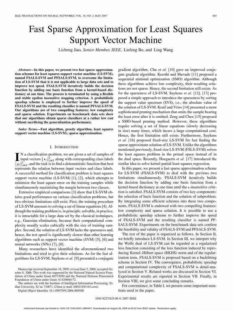
TABLE XIINUMBER OF SUPPORT VECTORS OBTAINED BY FSALS-SVM, PFSALS-SVM, LS-SVM, AND SVM ON THE TRAINING SET OF USPS DATA SET

TABLE XIIITRAINING TIME OBTAINED BY FSALS-SVM, PFSALS-SVM, LS-SVM, AND SVM ON THE TRAINING SET OF USPS DATA SET

TABLE XIVACCURACIES, NUMBER OF SUPPORT VECTORS, AND TRAINING TIME OBTAINED BY FSALS-SVM AND SVM ON MNIST1 DATA SET.

ACC DENOTES THE CLASSIFICATION ACCURACY ON TEST SET, NSV DENOTES THE NUMBER OF SUPPORT VECTORS ON TRAINING SET,AND TIME DENOTES THE CPU TIME IN SECONDS ON TRAINING SET

data sets, Ringnorm and Satimage, are used for this purpose. Foreach data set, is set to be a suitable value giving the best gen-eralization performance. Plots of the classification accuracy, thenumber of support vectors, and the training time as functions of

are shown in Figs. 1–3.We can see that the number of support vectors and the

training time of FSALS-SVM monotonously decrease withan increasing value of , which can be explicitly explainedby the meaning of . However, the classification accuracyof FSALS-SVM possibly suffers from an ascending and de-scending process with an increasing value of , which meansthat LS-SVM, i.e., FSALS-SVM with , may not be the

best choice if our purpose is to achieve the best generalizationperformance.

C. Comparisons With KMP and SGGP

The task of this section is to compare PSASLS-SVM withKMP and SGGP. All three algorithms use the probabilisticspeedup scheme with the random set of size 146. All the freeparameters are tuned using tenfold cross validation [35]. Theresults of the three algorithms on Ringnorm and USPS data setsare shown in Tables XVIII and XIX.

For Ringnorm data set, the classification accuracy of PF-SALS-SVM is slightly higher than KMP and SGGP. The



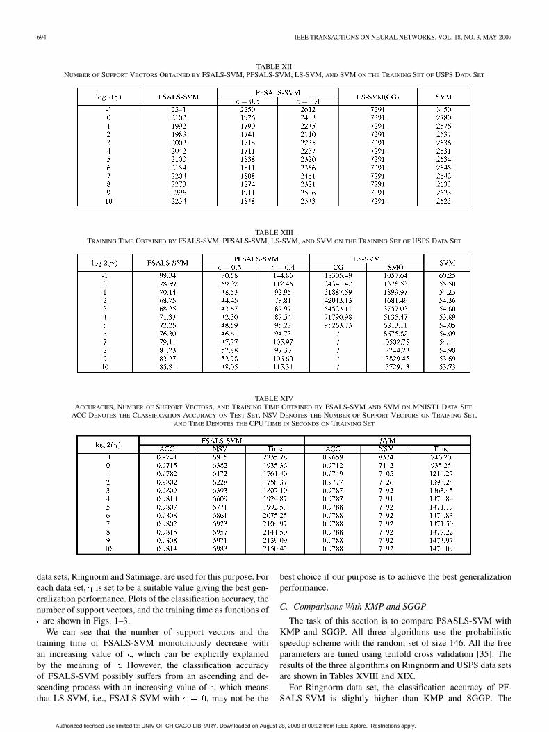
TABLE XVACCURACIES, NUMBER OF SUPPORT VECTORS, AND TRAINING TIME OBTAINED BY PFSALS-SVM ON MNIST1 DATA SET. ACCDENOTES THE CLASSIFICATION ACCURACY ON TEST SET, NSV DENOTES THE NUMBER OF SUPPORT VECTORS ON TRAINING SET,

AND TIME DENOTES THE CPU TIME IN SECONDS ON TRAINING SET

TABLE XVIACCURACIES, NUMBER OF SUPPORT VECTORS, AND TRAINING TIME OBTAINED BY PFSALS-SVM AND SVM ON MNIST DATA SET. ACC DENOTES

THE CLASSIFICATION ACCURACY ON TEST SET, NSV DENOTES THE NUMBER OF SUPPORT VECTORS ON TRAINING SET,AND TIME DENOTES THE CPU TIME IN SECONDS ON TRAINING SET

TABLE XVIIACCURACIES, NUMBER OF SUPPORT VECTORS, AND TRAINING TIME OBTAINED BY PFSALS-SVM ON MNIST DATA SET. ACC DENOTES THE CLASSIFICATION

ACCURACY ON TEST SET, NSV DENOTES THE NUMBER OF SUPPORT VECTORS ON TRAINING SET,AND TIME DENOTES THE CPU TIME IN SECONDS ON TRAINING SET

number of support vectors of PFSALS-SVM is more thanthat of KMP and SGGP, however, the training time of PF-SALS-SVM is comparable with that of KMP and significantlyshorter than that of SGGP. For USPS data set, PFSALS-SVMoutperforms KMP and SGGP in terms of the classificationaccuracy, the number of support vectors, and the training time.In particular, the training time of PFSALS-SVM is about 1/20that of KMP and 1/200 that of SGGP.

VIII. CONCLUSION

LS-SVM is a successful approach to classification, buttwo obvious limitations still exist. First, its computationalcomplexity usually scales cubically with the size of trainingsamples. Second, the solution of LS-SVM lacks the sparsenessand, hence, the test speed is very slow. This paper describesa fast greedy algorithm for LS-SVM, named FSALS-SVM,



Fig. 1. Variation of the classification accuracy of FSALS-SVM with parameter �. (a) Ringnorm data set with = 2 . (b) Statimage data set with = 2 .

Fig. 2. Variation of the number of support vectors of FSALS-SVM with parameter �. (a) Ringnorm data set with = 2 . (b) Statimage data set with = 2 .

Fig. 3. Variation of the training time of FSALS-SVM with parameter �. (a) Ringnorm data set with = 2 . (b) Statimage data set with = 2 .

TABLE XVIIIRESULTS OF PFSALS-SVM, KMP, AND SGGP ON RINGNORM DATA SET.

NSV DENOTES THE NUMBER OF SUPPORT VECTORS, ACC DENOTES

THE CLASSIFICATION ACCURACY, AND TIME DENOTES

THE TRAINING TIME IN SECONDS

which attempts to overcome the two limitations simultaneously.Using a probabilistic speedup scheme, we can further improvethe speed of FSALS-SVM and the resulting classifier is namedPFSALS-SVM. FSALS-SVM and PFSALS-SVM achieveboth low complexity and sparseness due to the introductionof -insensitive criterion. Extensive empirical comparisons

TABLE XIXRESULTS OF PFSALS-SVM, KMP, AND SGGP ON USPS DATA SET.NSV DENOTES THE NUMBER OF SUPPORT VECTORS, ACC DENOTES

THE CLASSIFICATION ACCURACY, AND TIME DENOTES

THE TRAINING TIME IN SECONDS

suggest that FSALS-SVM and PFSALS-SVM yield goodgeneralization performance on various classification problems.

ACKNOWLEDGMENT

The authors would lie to thank the three reviewers for theirhelpful comments that greatly improved this paper.



REFERENCES

[1] J. A. K. Suykens and J. Vandewalle, “Least squares support vector ma-chine classifiers,” Neural Process. Lett., vol. 9, no. 3, pp. 293–300,1999.

[2] T. Van Gestel, J. Suykens, G. Lanckriet, A. Lambrechts, B. De Moor,and J. Vandewalle, “Bayesian framework for least squares supportvector machine classifiers, Gaussian processes and kernel fisherdiscriminant analysis,” Neural Comput., vol. 15, no. 5, pp. 1115–1148,2002.

[3] T. Van Gestel, J. Suykens, B. Baesens, S. Viaene, J. Vanthienen, G.Dedene, B. De Moor, and J. Vandewalle, “Benchmarking least squaressupport vector machine classifiers,” Mach. Learn., vol. 54, no. 1, pp.5–32, 2004.

[4] L. V. Ferreira, E. Kaszkurewicz, and A. Bhaya, “Solving systems oflinear equations via gradient systems with discontinuous righthandsides: Application to LS-SVM,” IEEE Trans. Neural Netw., vol. 16,no. 2, pp. 501–505, Mar. 2005.

[5] V. Vapnik, The Nature of Statistical Learning Theory. New York:Springer-Verlag, 1995.

[6] ——, Statistical Learning Theory. New York: Wiley, 1998.[7] R. Neal, Bayesian Learning for Neural Networks. New York:

Springer-Verlag, 1996.[8] R. Ripley, Pattern Recognition and Neural Networks. Cambridge,

U.K.: Cambridge Univ. Press, 1996.[9] J. A. K. Suykens, L. Lukas, P. Van Dooren, B. De Moor, and J. Van-

dewalle, “Least squares support vector machine classifiers: A largescale algorithm,” in Proc. Euro. Conf. Circuit Theory Design, 1999,pp. 839–842.

[10] W. Chu, C. J. Ong, and S. S. Keerthy, “An improved conjugate gradientmethod scheme to the solution of least squares SVM,” IEEE Trans.Neural Netw., vol. 16, no. 2, pp. 498–501, Mar. 2005.

[11] S. S. Keerthi and S. K. Shevade, “SMO for least squares SVM formu-lations,” Neural Comput., vol. 15, pp. 487–507, 2003.

[12] J. A. K. Suykens, L. Lukas, and J. Vandewalle, “Sparse approximationusing least square vector machines,” in IEEE Proc. Int. Symp. CircuitsSyst., Genvea, Switzerland, 2000, pp. 757–760.

[13] J. A. K. Suykens, J. D. Brabanter, L. Lukas, and J. Vandewalle,“Weighted least squares support vector machines: Robustness andsparse approximation,” Neurocomput., vol. 48, pp. 85–105, 2002.

[14] B. J. de Kruif and T. J. A. de Vries, “Pruning error minimization in leastsquares support vector machines,” IEEE Trans. Neural Netw., vol. 14,no. 3, pp. 696–702, May 2004.

[15] X. Y. Zeng and X. W. Chen, “SMO-based pruning methods for sparseleast squares support vector machines,” IEEE Trans. Neural Netw., vol.16, no. 6, pp. 1541–1546, Nov. 2005.

[16] J. A. K. Suykens, T. Van Gestel, J. De Brabanter, B. De Moor, andJ. Vandewalle, Least Squares Support Vector Machines. Singapore:World Scientific, 2002.

[17] L. Hoegaerts, J. Suykens, J. Vandewalle, and B. De Moor, “Primalspace sparse kernel partial least squares regression for large scaleproblems,” in IEEE Proc. Int. Joint Conf. Neural Networks, 2004, pp.561–566.

[18] G. Gauwenberghs and T. Poggio, “Incremental and decremental sup-port vector machine learning,” in Proc. Neural Inf. Process. Syst., 2000,vol. 13, pp. 668–674.

[19] N. Aronszajn, “Theory of reproducting kernels,” Trans. Amer. Math.Soc., vol. 686, pp. 337–404, 1950.

[20] F. Girosi, “An equivalence between sparse approximation and supportvector machine,” Neural Comput., vol. 10, pp. 1455–1480, 1998.

[21] P. Vincent and Y. Bengio, “Kernel matching pursuit,” Mach. Learn.,vol. 48, pp. 165–187, 2001.

[22] J. Stoer and R. Bulirsch, Introduction to Numerical Analysis. NewYork: Springer-Verlag, 1993.

[23] J. H. Ma, J. Theiler, and S. Perkins, “Accurate on-line support vectorregression,” Neural Comput., vol. 15, pp. 2683–2703, 2003.

[24] L. Csató and M. Opper, “Sparse on-line Gaussian processes,” NeuralComput., vol. 14, pp. 641–668, 2002.

[25] X. D. Zhang, Matrix Analysis and Application. Beijing, China: Ts-inghua Univ. Press, 2004.

[26] R. Caruana, S. Lawrence, and L. Giles, “Overfitting in neural nets:Backpropagation, gradient, and early stopping,” in Proc. Neural Inf.Process. Syst., 2001, vol. 13, pp. 402–408.

[27] A. J. Smola and P. L. Bartlett, “Sparse greedy Gaussian process regres-sion,” in Proc. Neural Inf. Process. Syst., 2001, vol. 13, pp. 619–625.

[28] S. Mallat and Z. Zhang, “Matching pursuit with time-frequency dictio-naries,” IEEE Trans. Signal Process., vol. 41, no. 12, pp. 3397–3415,Dec. 1993.

[29] R. Rifkin and A. Klautau, “In defense of one-vs-all classification,” J.Mach. Learn. Res., vol. 5, pp. 101–141, 2004.

[30] L. Breiman, “Arcing classifiers,” Ann. Statist., vol. 26, no. 3, pp.801–809, 1998.

[31] D. Michie, D. J. Spiegelhalter, and C. C. Taylor, Machine Learning,Neural and Statistical Classification. Englewood Cliffs, NJ: PrenticeHall, 1994 [Online]. Available: ftp.ncc.up.pt/pub/statlog/

[32] Y. LeCun, B. Boser, J. S. Denker, D. Henderson, R. E. Howard, W.Hubbard, and L. D. Jackel, “Backpropagation applied to handwrittenzip code recognition,” Neural Comput., vol. 1, pp. 541–551, 1989.

[33] Y. LeCun, L. Bottou, Y. Bengio, and P. Haffner, “Gradient-basedlearning applied to document recognition,” Proc. IEEE, vol. 86, no.11, pp. 2278–2324, Nov. 1998.

[34] C.-C. Chang and C.-J. Lin, “LIBSVM: A library for support vector ma-chines” 2004 [Online]. Available: http://www.csie.ntu.edu.tw/~cjlin/libsvm

[35] L. F. Bo, L. Wang, and L. C. Jiao, “Feature scaling for kernel fisherdiscriminant analysis using leave-one-out cross validation,” NeuralComput., vol. 18, pp. 961–978, 2006.

Licheng Jiao (SM’89) was born in Shaanxi, China,on October 15, 1959. He received the B.S. degreefrom Shanghai Jiaotong University, Shanghai, China,in 1982, and the M.S. and Ph.D. degrees from Xi’anJiaotong University, Xi’an, China, in 1984 and 1990,respectively, all in electronical engineering.

From 1984 to 1986, he was an Assistant Professorin the Civil Aviation Institute of China, Tianjing,China. From 1990 to 1991, he was a PostdoctoralFellow in the National Key Laboratory for RadarSignal Processing, Xidian University, Xi’an, China.

Currently, he is the Dean of the Electronic Engineering School and the Directorof the Institute of Intelligent Information Processing, Xidian University. He isthe author of three books: Theory of Neural Network Systems (Xi’an, China:Xidian Univ. Press, 1990), Theory and Application on Nonlinear Transforma-tion Functions (Xi’an, China: Xidian Univ. Press, 1992), and Applications andImplementations of Neural Networks (Xi’an, China: Xidian Univ. Press, 1996).He is the author or coauthor of more than 150 scientific papers. His currentresearch interests include signal and image processing, nonlinear circuit andsystems theory, learning theory and algorithms, optimization problems, wavelettheory, and data mining.

Liefeng Bo was born in Xi’an, China, on March 26,1978. He received the B.S. degree from the Schoolof Science, Xidian University, Xi’an, China, in 2002,and he is currently working towards the Ph.D. degreein circuits and systems from the Institute of Intelli-gent Information Processing, Xidian University.

He has published several papers in some leadingjournals such as Neural Computation and IEEETRANSACTIONS ON NEURAL NETWORKS. His currentresearch interests include kernel-based learning,manifold learning, NNs, and computer version.

Ling Wang was born in Xi’an, China, on November10, 1978. She received the B.S. degree from theSchool of Science and the M.S. degree in computerscience from Xidian University, Xi’an, China, in2001 and 2005, respectively, where she is currentlyworking towards the Ph.D. degree in circuits andsystems at the Institute of Intelligent InformationProcessing.

Her current research interests include patternrecognition, statistical machine learning, and imageprocessing.


Documents

IEEE TRANSACTIONS ON NEURAL NETWORKS, VOL. · PDF fileand sparse solution. ... (SMO) algorithm. ... 2009 at 00:02 from IEEE Xplore. Restrictions apply. 686 IEEE TRANSACTIONS ON NEURAL