686 IEEE TRANSACTIONS ON NEURAL NETWORKS, VOL. 20, NO. …

686 IEEE TRANSACTIONS ON NEURAL NETWORKS, VOL. 20, NO. 4, APRIL 2009

Spurious Valleys in the Error Surface of RecurrentNetworks—Analysis and Avoidance

Jason Horn, Member, IEEE, Orlando De Jesús, Member, IEEE, and Martin T. Hagan, Member, IEEE

Abstract—This paper gives a detailed analysis of the error sur-faces of certain recurrent networks and explains some difficultiesencountered in training recurrent networks. We show that theseerror surfaces contain many spurious valleys, and we analyze themechanisms that cause the valleys to appear. We demonstrate thatthe principle mechanism can be understood through the analysisof the roots of random polynomials. This paper also provides sug-gestions for improvements in batch training procedures that canhelp avoid the difficulties caused by spurious valleys, thereby im-proving training speed and reliability.

Index Terms—Backpropagation, error surface, recurrent neuralnetworks, spurious minima, spurious valleys, training.

I. INTRODUCTION

R ECURRENT neural networks have been applied success-fully in the identification and control of dynamic systems

[18], prediction in financial markets [32], channel equalizationin communication systems [12], phase detection in power sys-tems [27], sorting [24], fault detection [6], speech recognition[13], [16], [31], handwriting recognition [17], learning of gram-mars in natural languages [29], and even the prediction of pro-tein structure in genetics [14]. However, even though these net-works have been widely used, the difficulty of recurrent net-work training has limited their widespread application [3], [9],[20]–[22].

One of the difficulties in training recurrent networks is theexistence of spurious local minima in the error surface. It hasbeen known for many years that even the error surfaces of mul-tilayer feedforward networks can have local minima. Sontag andSussman [33] showed that even networks without hidden layerscan have such spurious minima. They considered pattern recog-nition problems, in which sigmoid transfer functions were used.Bianchini et al. [5] discussed the problem of local minima inrecurrent neural networks. They restricted their analysis to thecase of recurrent networks used for recognition of “frames.” The

Manuscript received March 21, 2008; revised July 16, 2008 and October 06,2008; accepted November 10, 2008. First published March 06, 2009; currentversion published April 03, 2009.

J. Horn is with the Agilent Technologies High Frequency Technology Center,Santa Clara, CA 95051 USA (e-mail: [email protected]).

O. De Jesús is with the Research Department, Halliburton Energy Services,Dallas, TX 75006 USA (e-mail: [email protected]).

M. T. Hagan is with the School of Electrical and Computer Engineering,Oklahoma State University, Stillwater, OK 74078 USA (e-mail: [email protected]).

Color versions of one or more of the figures in this paper are available onlineat http://ieeexplore.ieee.org.

Digital Object Identifier 10.1109/TNN.2008.2012257

networks that they considered also used sigmoid transfer func-tions. Their analysis showed how the network architecture andthe learning environment both contributed to the complexity ofthe error surface. They showed that if the network architectureand the learning environment satisfy certain “recurrent networkassumptions,” then the error surface contains no local minima.However, these conditions for optimal learning are only suf-ficient, and satisfying the criteria may require networks withlarge input size based on the unfolding in time of the neuralnetwork. More recently, Gori and Sperduti [15] developed suffi-cient conditions which guarantee the absence of local minima ofthe error function in the case of learning directed acyclic graphswith recursive (related to recurrent) neural networks. They de-veloped a method for designing a neural architecture with alocal-minima-free error function for a given data set. As in pre-vious work, their networks used sigmoid transfer functions andperformed pattern recognition tasks.

There have been other approaches to recurrent networktraining that involve selecting the initial weights so that thechance of falling into a local minimum is minimized. Forexample, Wang and Chen [38] describe an automated pro-cedure that combines minimal model determination, weightinitialization, and performance optimization. This techniqueis designed for a specific network architecture that is used fordynamic system identification. Huang et al. [23] discuss theproblem of local minima in recurrent networks and proposean efficient structure and parameter learning algorithm forthe Jordan network. A key step in their procedure is a goodinitial guess for the network weights. Xiao et al. [39] proposea two-stage training process. In the first stage, particle swarmoptimization is used to locate an initial guess that will speednetwork convergence. In the second stage, a backpropagationalgorithm is used to train the network to convergence. All ofthese papers use weight initialization to attempt to avoid localminima in recurrent network error surfaces, but they do notexplain why the minima occur.

This paper will focus on recurrent networks that are used forsystem identification, control, filtering, prediction, and relatedtasks, which involve sequence processing and produce contin-uous outputs. The concepts discussed here apply to arbitraryrecurrent network architectures, although we will fully inves-tigate only simple networks. We will demonstrate that the errorsurfaces of recurrent networks have spurious valleys, which candisrupt in a significant way the training of recurrent networks.We suggest a newly discovered mechanism that can explain, atleast in part, the cause of spurious valleys in the error surfacesof recurrent networks. We show that this mechanism can evenproduce spurious valleys in a simple recurrent network with a

1045-9227/$25.00 © 2009 IEEE

Authorized licensed use limited to: Oklahoma State University. Downloaded on May 14, 2009 at 16:58 from IEEE Xplore. Restrictions apply.

HORN et al.: SPURIOUS VALLEYS IN THE ERROR SURFACE OF RECURRENT NETWORKS—ANALYSIS AND AVOIDANCE 687

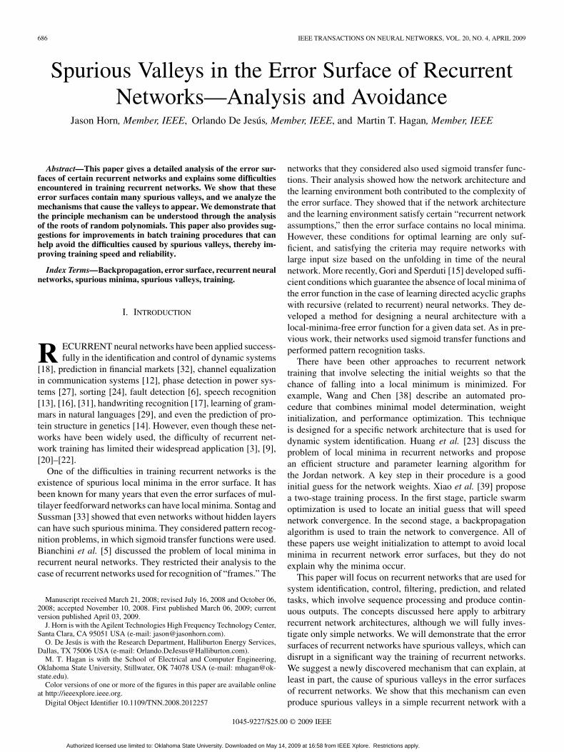
Fig. 1. Error profile.

linear transfer function and a single neuron. To our knowledge,this has not been previously reported in the literature. Based onour analysis of this mechanism, we will also propose modifiedtraining procedures that can provide improved convergence. Wewill demonstrate the operation of these modified training proce-dures on two simple recurrent networks.

II. PRELUDE

We begin with a description of how we encountered spuriousvalleys in the error surfaces of recurrent networks. Whiletraining a neural-network-based model reference controller[10], we found that the error sometimes increased duringtraining, although a line search minimization was being ex-ecuted at each iteration. In order to understand the failureof the line search, we plotted the error surface along thesearch direction. A typical profile is shown in Fig. 1. For thesystem shown, we have 65 weights being trained. The surfacewe present is along the direction of search [obtained by theBroyden–Fletcher–Goldfarb–Shanno (BFGS) quasi-Newtonalgorithm] through a 65-dimensional space. It is clear fromthis profile that any standard line search, using a combinationof interpolation and sectioning, will have great difficulty inlocating the minimum along the search direction. There aremany local minima contained in very narrow valleys. (Some ofthe valleys were found to have widths on the order of .) Inaddition, the bottom of the valleys are often cusps. (The neuralnetwork function is continuous and infinitely differentiable,so theoretically no cusps can exist. In practice, however, thevalleys are so narrow that they appear as cusps on the domainof double-precision numbers, and therefore, they are effectivelycusps for most training and analysis purposes.) We normallyassume that the minimum will occur at the point where thederivative is zero. However, for some of these valleys, thederivative continues to increase as we approach the minimum.Even if our line search were to locate the minimum, it is notclear that the minimum represents an optimal weight location.In fact, in the remainder of this paper, we will demonstrate thatspurious minima are introduced into the error surface due tocharacteristics of the input sequence.

In order to understand how spurious valleys can appear in theerror surface, we analyzed the surfaces for some very simplerecurrent networks. The idea was to find the simplest networkthat would produce the valleys. In the next section, we discuss a

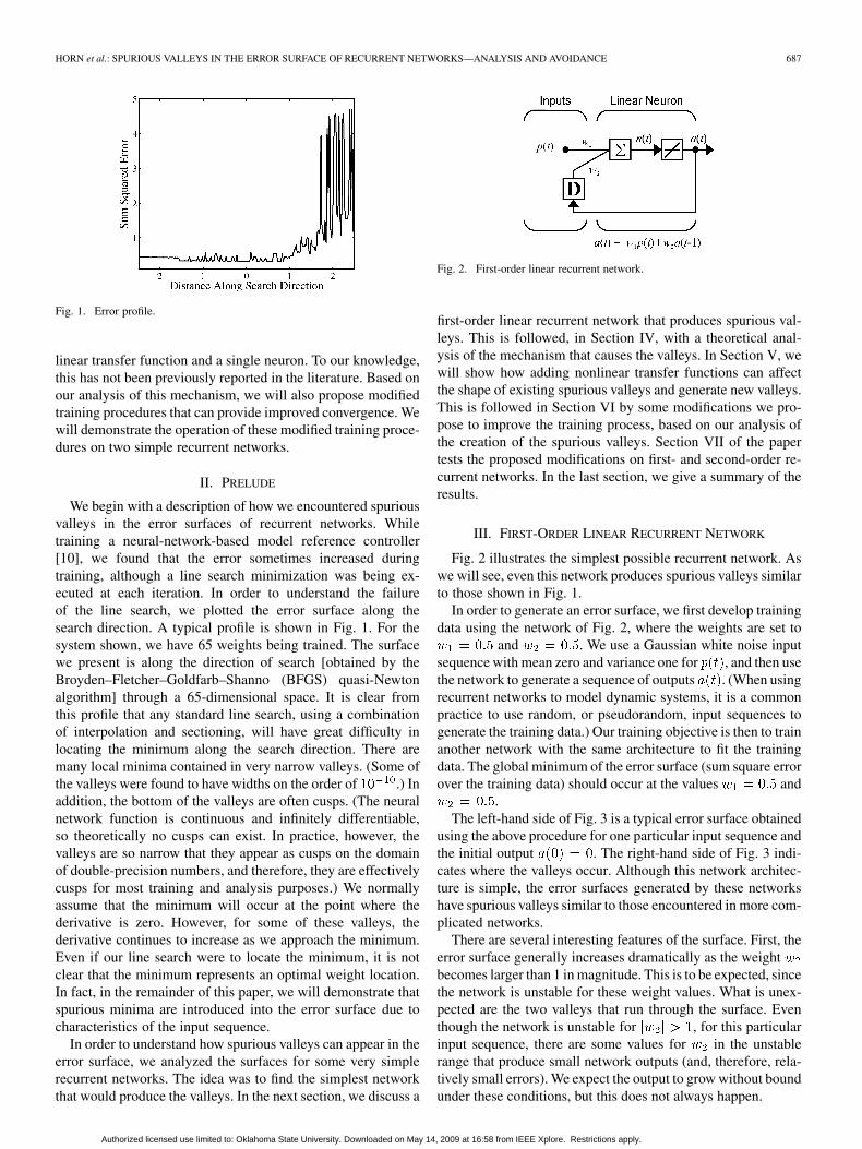
Fig. 2. First-order linear recurrent network.

first-order linear recurrent network that produces spurious val-leys. This is followed, in Section IV, with a theoretical anal-ysis of the mechanism that causes the valleys. In Section V, wewill show how adding nonlinear transfer functions can affectthe shape of existing spurious valleys and generate new valleys.This is followed in Section VI by some modifications we pro-pose to improve the training process, based on our analysis ofthe creation of the spurious valleys. Section VII of the papertests the proposed modifications on first- and second-order re-current networks. In the last section, we give a summary of theresults.

III. FIRST-ORDER LINEAR RECURRENT NETWORK

Fig. 2 illustrates the simplest possible recurrent network. Aswe will see, even this network produces spurious valleys similarto those shown in Fig. 1.

In order to generate an error surface, we first develop trainingdata using the network of Fig. 2, where the weights are set to

and . We use a Gaussian white noise inputsequence with mean zero and variance one for , and then usethe network to generate a sequence of outputs . (When usingrecurrent networks to model dynamic systems, it is a commonpractice to use random, or pseudorandom, input sequences togenerate the training data.) Our training objective is then to trainanother network with the same architecture to fit the trainingdata. The global minimum of the error surface (sum square errorover the training data) should occur at the values and

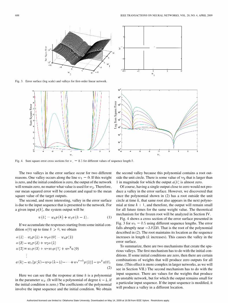
.The left-hand side of Fig. 3 is a typical error surface obtained

using the above procedure for one particular input sequence andthe initial output . The right-hand side of Fig. 3 indi-cates where the valleys occur. Although this network architec-ture is simple, the error surfaces generated by these networkshave spurious valleys similar to those encountered in more com-plicated networks.

There are several interesting features of the surface. First, theerror surface generally increases dramatically as the weightbecomes larger than 1 in magnitude. This is to be expected, sincethe network is unstable for these weight values. What is unex-pected are the two valleys that run through the surface. Eventhough the network is unstable for , for this particularinput sequence, there are some values for in the unstablerange that produce small network outputs (and, therefore, rela-tively small errors). We expect the output to grow without boundunder these conditions, but this does not always happen.



Fig. 3. Error surface (log scale) and valleys for first-order linear network.

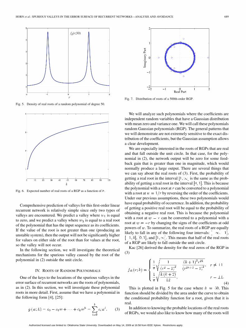
Fig. 4. Sum square error cross sections for � � �� for different values of sequence length �.

The two valleys in the error surface occur for two differentreasons. One valley occurs along the line . If this weightis zero, and the initial condition is zero, the output of the networkwill remain zero, no matter what value is used for . Therefore,our mean squared error will be constant and equal to the meansquare value of the target outputs.

The second, and more interesting, valley in the error surfaceis due to the input sequence that is presented to the network. Fora given input , the system output will be

(1)

If we accumulate the responses starting from some initial con-dition up to time , we obtain

...

(2)

Here we can see that the response at time is a polynomialin the parameter . (It will be a polynomial of degree , ifthe initial condition is zero.) The coefficients of the polynomialinvolve the input sequence and the initial condition. We obtain

the second valley because this polynomial contains a root out-side the unit circle. There is some value of that is larger than1 in magnitude for which the output is almost zero.

Of course, having a single output close to zero would not pro-duce a valley in the error surface. However, we discovered thatonce the polynomial shown in (2) has a root outside the unitcircle at time , that same root also appears in the next polyno-mial at time , and therefore, the output will remain smallfor all future times for the same weight value. The theoreticalmechanism for the frozen root will be analyzed in Section IV.

Fig. 4 shows a cross section of the error surface presented inFig. 3 for using different sequence lengths. The errorfalls abruptly near . That is the root of the polynomialdescribed in (2). The root maintains its location as the sequenceincreases in length ( increases). This causes the valley in theerror surface.

To summarize, there are two mechanisms that create the spu-rious valleys. The first mechanism has to do with the initial con-ditions. If some initial conditions are zero, then there are certaincombinations of weights that will produce zero outputs for alltime. (This effect is more complex in larger networks, as we willsee in Section VII.) The second mechanism has to do with theinput sequence. There are values for the weights that producean unstable network, but for which the output remains small fora particular input sequence. If the input sequence is modified, itwill produce a valley in a different location.



Fig. 5. Density of real roots of a random polynomial of degree 50.

Fig. 6. Expected number of real roots of a RGP as a function of �.

Comprehensive prediction of valleys for this first-order linearrecurrent network is relatively simple since only two types ofvalleys are encountered. We predict a valley where is equalto zero, and we predict a valley where is equal to a real rootof the polynomial that has the input sequence as its coefficients.If the value of the root is not greater than one (producing anunstable system), then the output will not be significantly higherfor values on either side of the root than for values at the root,so the valley will not occur.

In the following section, we will investigate the theoreticalmechanisms for the spurious valley caused by the root of thepolynomial in (2) outside the unit circle.

IV. ROOTS OF RANDOM POLYNOMIALS

One of the keys to the locations of the spurious valleys in theerror surface of recurrent networks are the roots of polynomials,as in (2). In this section, we will investigate these polynomialroots in more detail. First, assume that we have a polynomial inthe following form [4], [25]:

(3)

Fig. 7. Distribution of roots of a 500th-order RGP.

We will analyze such polynomials where the coefficients areindependent random variables that have a Gaussian distributionwith mean zero and variance one. We will call these polynomialsrandom Gaussian polynomials (RGP). The general patterns thatwe will demonstrate are not extremely sensitive to the exact dis-tribution of the coefficients, but the Gaussian assumption allowsa clear development.

We are especially interested in the roots of RGPs that are realand that fall outside the unit circle. In that case, for the poly-nomial in (2), the network output will be zero for some feed-back gain that is greater than one in magnitude, which wouldnormally produce a large output. There are several things thatwe can say about the real roots of (3). First, the probability ofgetting a real root in the interval is the same as the prob-ability of getting a real root in the interval . This is becausethe polynomial with a root at can be converted to a polynomialwith a root at by reversing the order of the coefficients.Under our previous assumptions, these two polynomials wouldhave equal probability of occurrence. In addition, the probabilityof getting a positive real root will be equal to the probability ofobtaining a negative real root. This is because the polynomialwith a root at can be converted to a polynomial with aroot at by changing the signs of the coefficients at oddpowers of . To summarize, the real roots of a RGP are equallylikely to fall in any of the following four intervals: ,

, , and . This means that half of the real rootsof a RGP are likely to fall outside the unit circle.

Kac [26] derived the density for the real zeros of the RGP in(3)

(4)This is plotted in Fig. 5 for the case where . This

function should be divided by the area under the curve to obtainthe conditional probability function for a root, given that it isreal.

In addition to knowing the probable locations of the real rootsof RGPs, we would also like to know how many of the roots will



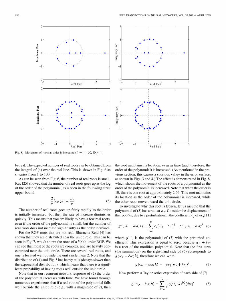
Fig. 8. Movement of roots as order is increased �� .

be real. The expected number of real roots can be obtained fromthe integral of (4) over the real line. This is shown in Fig. 6 as

varies from 1 to 100.As can be seen from Fig. 6, the number of real roots is small.

Kac [25] showed that the number of real roots goes up as the logof the order of the polynomial, as is seen in the following strictupper bound:

(5)

The number of real roots goes up fairly rapidly as the orderis initially increased, but then the rate of increase diminishesquickly. This means that you are likely to have a few real roots,even if the order of the polynomial is small, but the number ofreal roots does not increase significantly as the order increases.

For the RGP roots that are not real, Bharucha-Reid [4] hasshown that they are distributed near the unit circle. This can beseen in Fig. 7, which shows the roots of a 500th-order RGP. Wecan see that most of the roots are complex, and are heavily con-centrated near the unit circle. There are several real roots, andone is located well outside the unit circle, near 2. Note that thedistribution of (4) and Fig. 5 has heavy tails (decays slower thanthe exponential distribution), which means that there is a signif-icant probability of having roots well outside the unit circle.

Note that in our recurrent network response of (2) the orderof the polynomial increases with time. We have found throughnumerous experiments that if a real root of the polynomial fallswell outside the unit circle (e.g., with a magnitude of 2), then

the root maintains its location, even as time (and, therefore, theorder of the polynomial) is increased. (As mentioned in the pre-vious section, this causes a spurious valley in the error surface,as shown in Figs. 3 and 4.) The effect is demonstrated in Fig. 8,which shows the movement of the roots of a polynomial as theorder of the polynomial is increased. Note that when the order is10, there is one root at approximately 2.66. This root maintainsits location as the order of the polynomial is increased, whilethe other roots move toward the unit circle.

To investigate why this root is frozen, let us assume that thepolynomial of (3) has a root at . Consider the displacement ofthe root , due to a perturbation in the coefficient of [11]

(6)

where is the polynomial of (3) with the perturbed co-efficient. This expression is equal to zero, becauseis a root of the modified polynomial. Note that the first term(the summation) on the right-hand side of (6) corresponds to

, therefore we can write

(7)

Now perform a Taylor series expansion of each side of (7)

(8)



where the term is missing from the summation becauseis a root of , and

(9)

If we now set (8) equal to (9) and take the limit as , andtherefore, also , go to zero, we find

(10)

or

(11)

This tells us the sensitivity of the root location, as a functionof one of the coefficients in the polynomial. It is related to thecondition of the polynomial, which is defined in [11].

To relate this result to the recurrent network response of (2),we will first assume that and . (This willsimplify the development without changing the overall conclu-sions.) The resulting network response will be

(12)

If we equate this expression with (3), we see that

(13)

Now consider the coefficient . This is the lastinput to come into the network, and it increases the order of thepolynomial by 1. When , all previous rootsare unchanged. The sensitivity of a previous root to changes inthis coefficient is given by (11)

(14)

The denominator in this term is the first derivative of the poly-nomial , evaluated at the root

(15)

If the coefficients are random with mean zero and variance 1,then this term has variance given by

(16)

If the root is greater than 1 in magnitude, then this variancewill be very large even for moderate values of . This means thatit is highly likely that will be very large, and, based

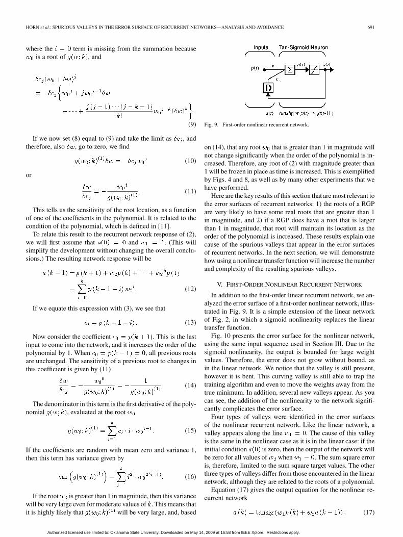
Fig. 9. First-order nonlinear recurrent network.

on (14), that any root that is greater than 1 in magnitude willnot change significantly when the order of the polynomial is in-creased. Therefore, any root of (2) with magnitude greater than1 will be frozen in place as time is increased. This is exemplifiedby Figs. 4 and 8, as well as by many other experiments that wehave performed.

Here are the key results of this section that are most relevant tothe error surfaces of recurrent networks: 1) the roots of a RGPare very likely to have some real roots that are greater than 1in magnitude, and 2) if a RGP does have a root that is largerthan 1 in magnitude, that root will maintain its location as theorder of the polynomial is increased. These results explain onecause of the spurious valleys that appear in the error surfacesof recurrent networks. In the next section, we will demonstratehow using a nonlinear transfer function will increase the numberand complexity of the resulting spurious valleys.

V. FIRST-ORDER NONLINEAR RECURRENT NETWORK

In addition to the first-order linear recurrent network, we an-alyzed the error surface of a first-order nonlinear network, illus-trated in Fig. 9. It is a simple extension of the linear networkof Fig. 2, in which a sigmoid nonlinearity replaces the lineartransfer function.

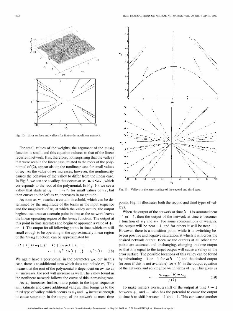
Fig. 10 presents the error surface for the nonlinear network,using the same input sequence used in Section III. Due to thesigmoid nonlinearity, the output is bounded for large weightvalues. Therefore, the error does not grow without bound, asin the linear network. We notice that the valley is still present,however it is bent. This curving valley is still able to trap thetraining algorithm and even to move the weights away from thetrue minimum. In addition, several new valleys appear. As youcan see, the addition of the nonlinearity to the network signifi-cantly complicates the error surface.

Four types of valleys were identified in the error surfacesof the nonlinear recurrent network. Like the linear network, avalley appears along the line . The cause of this valleyis the same in the nonlinear case as it is in the linear case: if theinitial condition is zero, then the output of the network willbe zero for all values of when . The sum square erroris, therefore, limited to the sum square target values. The otherthree types of valleys differ from those encountered in the linearnetwork, although they are related to the roots of a polynomial.

Equation (17) gives the output equation for the nonlinear re-current network

(17)



Fig. 10. Error surface and valleys for first-order nonlinear network.

For small values of the weights, the argument of the tansigfunction is small, and this equation reduces to that of the linearrecurrent network. It is, therefore, not surprising that the valleysthat were seen in the linear case, related to the roots of the poly-nomial of (2), appear also in the nonlinear case for small valuesof . As the value of increases, however, the nonlinearitycauses the behavior of the valley to differ from the linear case.In Fig. 3, we can see a valley that occurs at , whichcorresponds to the root of the polynomial. In Fig. 10, we see avalley that starts at for small values of , butthen curves to the left as increases in magnitude.

As soon as reaches a certain threshold, which can be de-termined by the magnitude of the terms in the input sequenceand the magnitude of at which the valley occurs, the outputbegins to saturate at a certain point in time as the network leavesthe linear operating region of the tansig function. The output atthis point in time saturates and begins to approach a value ofor . The output for all following points in time, which are stillsmall enough to be operating in the approximately linear regionof the tansig function, can be approximated by

(18)

We again have a polynomial in the parameter , but in thiscase, there is an additional term which does not include . Thismeans that the root of the polynomial is dependent on , so as

increases, the root will increase as well. The valley found inthe nonlinear network follows the curve of this increasing root.

As increases further, more points in the input sequencewill saturate and cause additional valleys. This brings us to thethird type of valley, which occurs as and increase enoughto cause saturation in the output of the network at most time

Fig. 11. Valleys in the error surface of the second and third type.

points. Fig. 11 illustrates both the second and third types of val-leys.

When the output of the network at time is saturated nearor , then the output of the network at time becomes

a function of and . For some combinations of weights,the output will be near , and for others it will be near .However, there is a transition point, while it is switching be-tween positive and negative saturation, at which it will cross thedesired network output. Because the outputs at all other timepoints are saturated and unchanging, changing this one outputso that it is equal to the target output will cause a valley in theerror surface. The possible locations of this valley can be foundby substituting or for and the desired output(or zero if this is not available) for in the output equationof the network and solving for in terms of . This gives us

(19)

To make matters worse, a shift of the output at timebetween and also has the potential to cause the outputat time to shift between and . This can cause another



Fig. 12. Error surface and valleys for small � (fourth type of valley) for thefirst-order nonlinear network.

valley, and also can cause the output at time to shift be-tween and . This cycle has the potential to continue untilthe final time point, so a single shift at time in an input se-quence of length has the potential to cause valleysnear the line given by (19).

Fortunately, not all of these potential valleys actually appearon the error surface. To determine which valleys will occur, asimple algorithm can be written which keeps track of the sign ofthe output at each time and determines which outputs will shiftbetween and as varies from to 0 and from0 to . Only the outputs that actually shift will cause valleysto occur. Using this method, we were able to predict accuratelythe locations of all valleys of this type that actually would occurfor a given input/output sequence of training data.

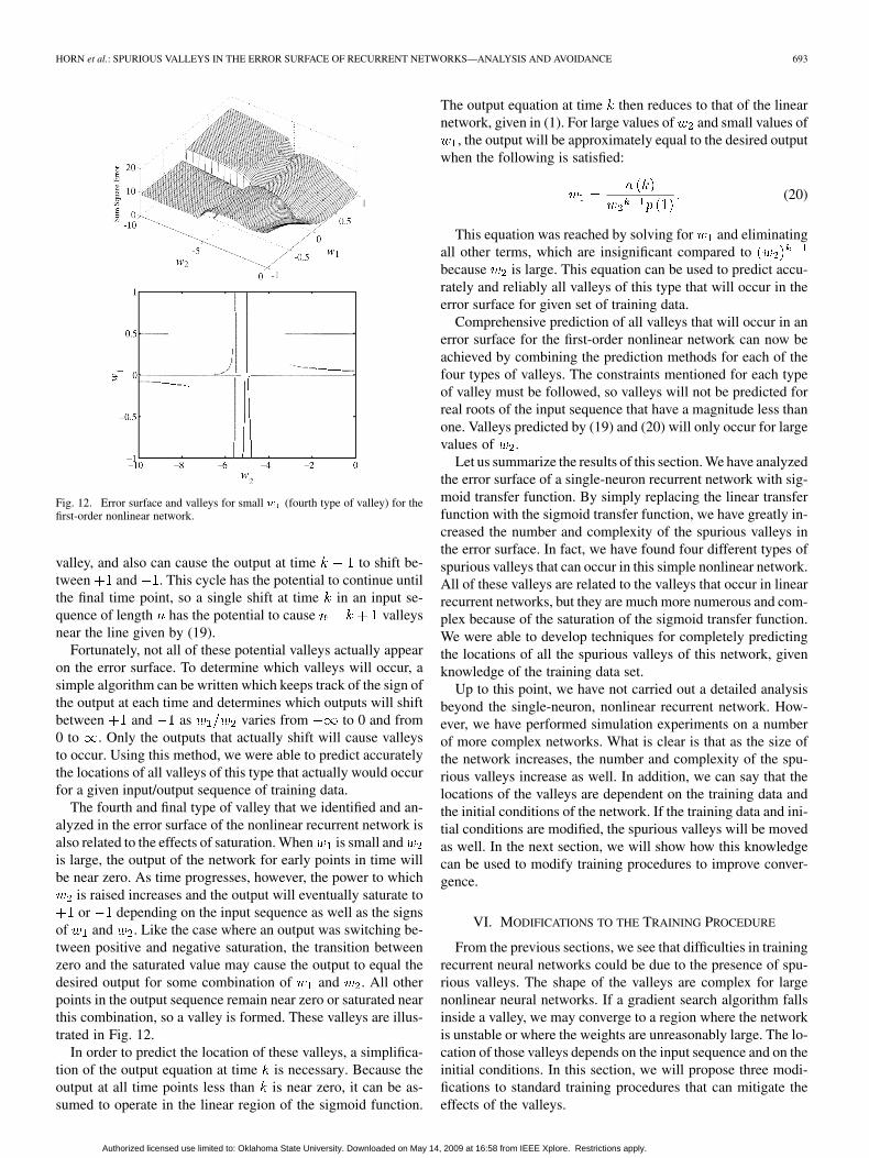
The fourth and final type of valley that we identified and an-alyzed in the error surface of the nonlinear recurrent network isalso related to the effects of saturation. When is small andis large, the output of the network for early points in time willbe near zero. As time progresses, however, the power to which

is raised increases and the output will eventually saturate toor depending on the input sequence as well as the signs

of and . Like the case where an output was switching be-tween positive and negative saturation, the transition betweenzero and the saturated value may cause the output to equal thedesired output for some combination of and . All otherpoints in the output sequence remain near zero or saturated nearthis combination, so a valley is formed. These valleys are illus-trated in Fig. 12.

In order to predict the location of these valleys, a simplifica-tion of the output equation at time is necessary. Because theoutput at all time points less than is near zero, it can be as-sumed to operate in the linear region of the sigmoid function.

The output equation at time then reduces to that of the linearnetwork, given in (1). For large values of and small values of

, the output will be approximately equal to the desired outputwhen the following is satisfied:

(20)

This equation was reached by solving for and eliminatingall other terms, which are insignificant compared tobecause is large. This equation can be used to predict accu-rately and reliably all valleys of this type that will occur in theerror surface for given set of training data.

Comprehensive prediction of all valleys that will occur in anerror surface for the first-order nonlinear network can now beachieved by combining the prediction methods for each of thefour types of valleys. The constraints mentioned for each typeof valley must be followed, so valleys will not be predicted forreal roots of the input sequence that have a magnitude less thanone. Valleys predicted by (19) and (20) will only occur for largevalues of .

Let us summarize the results of this section. We have analyzedthe error surface of a single-neuron recurrent network with sig-moid transfer function. By simply replacing the linear transferfunction with the sigmoid transfer function, we have greatly in-creased the number and complexity of the spurious valleys inthe error surface. In fact, we have found four different types ofspurious valleys that can occur in this simple nonlinear network.All of these valleys are related to the valleys that occur in linearrecurrent networks, but they are much more numerous and com-plex because of the saturation of the sigmoid transfer function.We were able to develop techniques for completely predictingthe locations of all the spurious valleys of this network, givenknowledge of the training data set.

Up to this point, we have not carried out a detailed analysisbeyond the single-neuron, nonlinear recurrent network. How-ever, we have performed simulation experiments on a numberof more complex networks. What is clear is that as the size ofthe network increases, the number and complexity of the spu-rious valleys increase as well. In addition, we can say that thelocations of the valleys are dependent on the training data andthe initial conditions of the network. If the training data and ini-tial conditions are modified, the spurious valleys will be movedas well. In the next section, we will show how this knowledgecan be used to modify training procedures to improve conver-gence.

VI. MODIFICATIONS TO THE TRAINING PROCEDURE

From the previous sections, we see that difficulties in trainingrecurrent neural networks could be due to the presence of spu-rious valleys. The shape of the valleys are complex for largenonlinear neural networks. If a gradient search algorithm fallsinside a valley, we may converge to a region where the networkis unstable or where the weights are unreasonably large. The lo-cation of those valleys depends on the input sequence and on theinitial conditions. In this section, we will propose three modi-fications to standard training procedures that can mitigate theeffects of the valleys.



Fig. 13. Error surface for first-order nonlinear network for different input se-quence.

A. Proposed Solutions

In this section, we will propose three variations to the stan-dard batch training algorithms for recurrent networks. Thesevariations include regularization, switching training sequences,and randomly setting initial conditions.

If we compare the linear and nonlinear cases from Sections IIIand V, we notice that the linear case has a natural way of al-lowing convergence to the optimal weights, because largerweights generate large outputs. The farther we move fromthe stable region, the larger the gradient will become. A gra-dient-descent algorithm would generally move the weightstoward the stable region. This effect does not occur in thenonlinear networks. However, we can obtain a similar effect ifwe combine regularization [30] with our mean square error per-formance function. In other words, we can use the performancefunction

(21)

where SSE is the sum squared errors and SSW is the sumsquared weights. This performance function would help toforce the weights back into the stable region, because it wouldoverwhelm the spurious valleys for large values of the weights.We can decrease the regularization factor during training toensure that we do not bias the final trained weights.

Fig. 14. Error surface using sequence averaging.

Another technique for improved training involves using morethan one training sequence. Fig. 13 presents the error surfacefor the nonlinear network of Fig. 9, using a different trainingsequence. The valley that appeared in Fig. 10 has moved to adifferent region of . For any two random input sequences,the valleys will appear in different locations.

This suggests another technique for improved training. Wecould use multiple training sequences. Because valleys are se-quence dependent, we can use one sequence for a given numberof epochs and then alternate to a new sequence. If we becometrapped in a spurious valley, that valley will disappear when thenew sequence is presented.

Another implementation of multiple sequences could be se-quence averaging. We could compute the gradients for multiplesequences and then move in the direction of the average. Fig. 14presents an average error surface for five sequences. This figuredemonstrates how the spurious valleys are reduced in amplitude.

Another method to move the valleys is to use random initialconditions. Fig. 15 shows how the error surface is changed whenwe set the initial condition to . The valley at ,which we discussed earlier, is missing. In later experiments withlarger networks, we found that the valleys do not always disap-pear when nonzero initial conditions are used. They are oftenonly moved to new locations. A better approach would be touse different small random initial conditions at different stagesof training. We could switch the initial conditions in combina-tion with the switching of sequences.



Fig. 15. Error surface using �� .

In all, we have four proposed training modifications. For easeof reference, we will label them as follows: switching sequences(SS), averaging sequences (AS), regularization (REG), nonzeroinitial conditions (IC).

VII. TEST RESULTS

In this section, we will test the training modifications thatwere proposed in the previous section. For these tests, we willtrain the nonlinear network shown in Section V (and a morecomplex, second-order network) using the standard gradient-de-scent algorithm with a golden section line search. We will notworry about using the most sophisticated training algorithm.Rather, the objective will be to verify the ability of the newprocedures to improve training performance. The results ob-tained with the basic gradient-descent algorithm will be ourbaseline. Other tests will be performed for each one of the pro-posed modifications. For the REG test, we divided by 1.2 ateach epoch. For the IC method, we set all layer initial condi-tions to 0.2. One test was performed using all three methods.We called this training procedure the “multiple” method. Forall tests, the gradient is computed using the real-time recurrentlearning method described in [7], [8], [19], and [34]–[36]. Abatch gradient is used, which encompasses the full length of thetraining sequence.

TABLE ICONVERGENCE PERCENTAGES FOR SINGLE-NEURON

RECURRENT NETWORK TRAINING

TABLE IICONVERGENCE PERCENTAGES FOR TWO-NEURON

RECURRENT NETWORK TRAINING

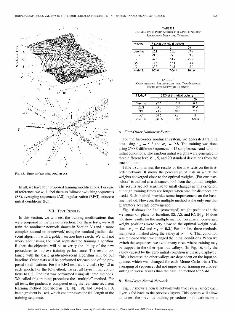
A. First-Order Nonlinear System

For the first-order nonlinear system, we generated trainingdata using and . The training was doneusing 25 000 different sequences of 15 samples each and randominitial conditions. The random initial weights were generated inthree different levels: 1, 5, and 20 standard deviations from thetrue solution.

Table I summarizes the results of the first tests on the first-order network. It shows the percentage of tests in which theweights converged close to the optimal weights. (For our tests,“close” is defined as a distance of 0.5 from the optimal weights.The results are not sensitive to small changes in this criterion,although training times are longer when smaller distances areused.) Each method provides some improvement on the base-line method. However, the multiple method is the only one thatguarantees accurate convergence.

Fig. 16 shows the final (converged) weight positions in theversus plane for baseline, SS, AS, and IC. (Fig. 16 does

not show results for the multiple method, because all convergedweight positions were very close to the optimal weight posi-tion— and .) For the first three methods,many tests finished along the valley at . That conditionwas removed when we changed the initial conditions. When weswitch the sequences, we avoid many cases where training maybe trapped in the other spurious valleys. (In Fig. 16, only thevalley caused by the zero initial condition is clearly displayed.This is because the other valleys are dependent on the input se-quence, which was changed for each Monte Carlo trial.) Theaveraging of sequences did not improve our training results, re-sulting in worse results than the baseline method for 5 std.

B. Two-Layer Neural Network

Fig. 17 shows a neural network with two layers, where eachlayer is fed back to the previous layers. This system will allowus to test the previous training procedure modifications on a



Fig. 16. Final weight positions in the � versus � plane for 5 std.

more complex system. For these tests, we generated trainingdata using the following weights:

Table II shows the percentage of weights close to the finalweights (within a distance of 0.5) after the training process.For this neural network architecture, regularization resulted ina success rate of over 90%. However, it is again the multiplemethod that guarantees the best convergence.

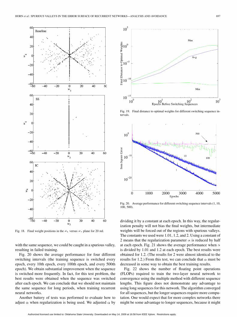
Fig. 18 presents the final weight positions in the versusplane for the baseline, SS, and IC training methods. For

the baseline training method, we notice the presence of threevalleys (due to zero initial conditions) where the training con-verged. The SS method can eliminate the diagonal valleys dueto the initial conditions, as well as the valleys due to the inputsequence. However, the valley along remains. When weset the initial layer conditions to 0.2, we can see from the lastfigure that although the valley at is removed, two newvalleys appear. This demonstrates that setting the initial condi-tions to nonzero values does not necessarily remove spurious

Fig. 17. Two-layer nonlinear model.

valleys. It may just move them to new locations. This suggeststhat we should vary the initial conditions whenever we switchthe training sequence.

Fig. 19 shows how the final distance to the optimal weightsis affected by the switching sequence interval. While trainingfor 10 000 epochs, we switched the training sequence every 1,10, 100, 500, and 1000 epochs. Frequent changes consistentlyresulted in more accurate final weights. If training continues



Fig. 18. Final weight positions in the � versus � plane for 20 std.

with the same sequence, we could be caught in a spurious valley,resulting in failed training.

Fig. 20 shows the average performance for four differentswitching intervals (the training sequence is switched everyepoch, every 10th epoch, every 100th epoch, and every 500thepoch). We obtain substantial improvement when the sequenceis switched more frequently. In fact, for this test problem, thebest results were obtained when the sequence was switchedafter each epoch. We can conclude that we should not maintainthe same sequence for long periods, when training recurrentneural networks.

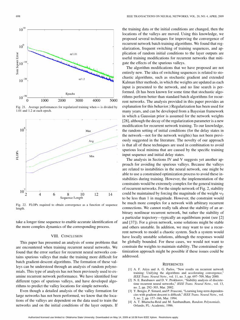
Another battery of tests was performed to evaluate how toadjust when regularization is being used. We adjusted by

Fig. 19. Final distance to optimal weights for different switching sequence in-tervals.

Fig. 20. Average performance for different switching sequence intervals (1, 10,100, 500).

dividing it by a constant at each epoch. In this way, the regular-ization penalty will not bias the final weights, but intermediateweights will be forced out of the regions with spurious valleys.The constants we used were 1.01, 1.2, and 2. Using a constant of2 means that the regularization parameter is reduced by halfat each epoch. Fig. 21 shows the average performance whenis divided by 1.01 and 1.2 at each epoch. The best results wereobtained for 1.2. (The results for 2 were almost identical to theresults for 1.2.) From this test, we can conclude that must bedecreased in some way to obtain the best training results.

Fig. 22 shows the number of floating point operations(FLOPs) required to train the two-layer neural network toconvergence using the multiple method with different sequencelengths. This figure does not demonstrate any advantage tousing long sequences for this network. The algorithm convergedfor all sequences, but the longer sequences require more compu-tation. One would expect that for more complex networks theremight be some advantage to longer sequences, because it might



Fig. 21. Average performances for regularized training when � is divided by1.01 and 1.2 at each epoch.

Fig. 22. FLOPs required to obtain convergence as a function of sequencelength.

take a longer time sequence to enable accurate identification ofthe more complex dynamics of the corresponding process.

VIII. CONCLUSION

This paper has presented an analysis of some problems thatare encountered when training recurrent neural networks. Wefound that the error surface for recurrent neural networks con-tains spurious valleys that make the training more difficult forbatch gradient-descent algorithms. The formation of these val-leys can be understood through an analysis of random polyno-mials. This type of analysis has not been previously used to ex-amine recurrent network performance. We have identified fourdifferent types of spurious valleys, and have developed algo-rithms to predict the valley locations for simple networks.

Even though a detailed analysis of the valley formation forlarge networks has not been performed, we know that the loca-tions of the valleys are dependent on the data used to train thenetworks and on the initial conditions of the layer outputs. If

the training data or the initial conditions are changed, then thelocations of the valleys are moved. Using this knowledge, weproposed several techniques for improving the convergence ofrecurrent network batch training algorithms. We found that reg-ularization, frequent switching of training sequences, and ap-plication of random initial conditions to the layer outputs areuseful training modifications for recurrent networks that miti-gate the effects of the spurious valleys.

The algorithm modifications that we have proposed are notentirely new. The idea of switching sequences is related to sto-chastic algorithms, such as stochastic gradient and extendedKalman filter methods, in which the weights are updated as eachinput is presented to the network, and no line search is per-formed. (It has been known for some time that stochastic algo-rithms perform better than standard batch algorithms for recur-rent networks. The analysis provided in this paper provides anexplanation for this behavior.) Regularization has been used formany years, and can be developed from a Bayesian frameworkin which a Gaussian prior is assumed for the network weights[28], although the decay of the regularization parameter is a newmodification for recurrent network training. To our knowledge,the random setting of initial conditions (for the delay states inthe network—not for the network weights) has not been previ-ously suggested in the literature. The novelty of our approachis that all of these techniques are used in combination to avoidspurious local minima that are caused by the specific traininginput sequence and initial delay states.

The analysis in Sections IV and V suggests yet another ap-proach for avoiding the spurious valleys. Because the valleysare related to instabilities in the neural network, one might beable to use a constrained optimization process to avoid these in-stabilities during training. However, the implementation of theconstraints would be extremely complex for the general trainingof recurrent networks. For the simple network of Fig. 2, stabilitycould be maintained by forcing the magnitude of the weightto be less than 1 in magnitude. However, the constraint wouldbe much more complex for a network with arbitrary recurrentconnections. We cannot really talk about the stability of an ar-bitrary nonlinear recurrent network, but rather the stability ofa particular trajectory—typically an equilibrium point (see [2]and [37]). For a given network, some solutions might be stableand others unstable. In addition, we may want to use a recur-rent network to model a chaotic system. Such a system wouldhave locally unstable solutions, although the responses wouldbe globally bounded. For these cases, we would not want toconstrain the weights to maintain stability. The constrained op-timization approach might be possible if these issues could beaddressed.

REFERENCES

[1] A. F. Atiya and A. G. Parlos, “New results on recurrent networktraining: Unifying the algorithms and accelerating convergence,”IEEE Trans. Neural Netw., vol. 11, no. 3, pp. 697–709, May 2000.

[2] N. E. Barabanov and D. V. Prokhorov, “Stability analysis of discrete-time recurrent neural networks,” IEEE Trans. Neural Netw., vol. 13,no. 2, pp. 292–303, Mar. 2002.

[3] Y. Bengio, P. Simard, and P. Frasconi, “Learning long-term dependen-cies with gradient descent is difficult,” IEEE Trans. Neural Netw., vol.5, no. 2, pp. 157–166, Mar. 1994.

[4] A. T. Bharucha-Reid and M. Sambandham, Random Polynomials.Orlando, FL: Academic, 1986.



[5] M. Bianchini, M. Gori, and M. Maggini, “On the problem of localminima in recurrent neural networks,” IEEE Trans. Neural Netw., vol.5, no. 2, pp. 167–177, Mar. 1994.

[6] G. Chengyu and K. Danai, “Fault diagnosis of the IFAC benchmarkproblem with a model-based recurrent neural network,” in Proc. IEEEInt. Conf. Control Appl., 1999, vol. 2, pp. 1755–1760.

[7] O. De Jesús, “Training general dynamic neural networks,” Ph.D. dis-sertation, Schl. Electr. Comput. Eng., Oklahoma State Univ., Stillwater,OK, 2002.

[8] O. De Jesús and M. T. Hagan, “Backpropagation algorithms for a broadclass of dynamic networks,” IEEE Trans. Neural Netw., vol. 18, no. 1,pp. 14–27, Jan. 2007.

[9] O. De Jesús, J. M. Horn, and M. T. Hagan, “Analysis of recurrent net-work training and suggestions for improvements,” in Proc. INNS-IEEEInt. Joint Conf. Neural Netw., Washington, DC, Jul. 2001, vol. 4, pp.2632–2637.

[10] O. De Jesús, A. Pukrittayakamee, and M. T. Hagan, “A comparisonof neural network control algorithms,” in Proc. INNS-IEEE Int. JointConf. Neural Netw., Washington, DC, Jul. 2001, vol. 1, pp. 521–526.

[11] R. T. Farouki and V. T. Rajan, “On the numerical condition of polyno-mials in Bernstein form,” Comput.-Aided Geometric Des., vol. 4, pp.191–216, 1987.

[12] J. Feng, C. K. Tse, and F. C. M. Lau, “A neural-network-basedchannel-equalization strategy for chaos-based communication sys-tems,” IEEE Trans. Circuits Syst. I: Fundam. Theory Appl., vol. 50,no. 7, pp. 954–957, Jul. 2003.

[13] S. Fernández, A. Graves, and J. Schmidhuber, “Sequence labellingin structured domains with hierarchical recurrent neural networks,” inProc. 20th Int. Joint Conf. Artif. Intell., Hyderabad, India, 2007, pp.774–779.

[14] P. Gianluca, D. Przybylski, B. Rost, and P. Baldi, “Improving the pre-diction of protein secondary structure in three and eight classes usingrecurrent neural networks and profiles,” Proteins: Structure, Function,Genetics, vol. 47, no. 2, pp. 228–235, 2002.

[15] M. Gori and A. Sperduti, “The loading problem for recursive neuralnetworks,” Neural Netw., vol. 18, pp. 1064–1079, 2005.

[16] A. Graves, S. Fernández, F. Gomez, and J. Schmidhuber, “Connec-tionist temporal classification: Labelling unsegmented sequence datawith recurrent neural nets,” in Proc. 23rd Int. Conf. Mach. Learn., Pitts-burgh, PA, 2006, pp. 369–376.

[17] A. Graves, S. Fernández, M. Liwicki, H. Bunke, and J. Schmidhuber,“Unconstrained on-line handwriting recognition with recurrent neuralnetworks,” Advances in Neural Information Processing Systems, vol.20, pp. 577–584, 2008.

[18] M. T. Hagan and H. B. Demuth, “Neural networks for control,” in Proc.Amer. Control Conf., San Diego, CA, 1999, pp. 1642–1656.

[19] M. T. Hagan, O. De Jesús, and R. Schultz, “Training recurrent networksfor filtering and control,” in Recurrent Neural Networks: Design andApplications, L. Medsker and L. C. Jain, Eds. Boca Raton, FL: CRCPress, 1999, ch. 12, pp. 311–340.

[20] S. Hochreiter, “Untersuchungen Zudynamischen Neuronalen Netzen,”Diploma, Technische Universitat Munchen, Institut fur Informatik,Munich, Germany, 1991.

[21] S. Hochreiter and J. Schmidhuber, “Long short-term memory,” NeuralComput., vol. 9, no. 8, pp. 1735–1780, 1997.

[22] J. Horn and M. Hagan, “Analysis of the error surface of simple recurrentneural networks,” in Intelligent Engineering Systems Through ArtificialNeural Networks (ANNIE2004). New York: ASME Press, 2004, vol.14.

[23] T.-Y. Huang, C. J. Li, and T.-W. Hsu, “Structure and parameterlearning algorithm of Jordan type recurrent neural networks,” in Proc.Int. Joint Conf. Neural Netw., Orlando, FL, Aug. 12–17, 2007, pp.1819–1824.

[24] Jayadeva and S. A. Rahman, “A neural network with O(N) neurons forranking N numbers in O(1/N) time,” IEEE Trans. Circuits Syst. I: Reg.Papers, vol. 51, no. 10, pp. 2044–2051, Oct. 2004.

[25] M. Kac, “On the average number of real roots of a random algebraicequation,” Bull. Amer. Math. Soc., vol. 49, pp. 314–320, 1943.

[26] M. Kac, Probability and Related Topics in the Physical Sciences, 1sted. New York: Interscience, 1960.

[27] I. Kamwa, R. Grondin, V. K. Sood, C. Gagnon, V. T. Nguyen, and J.Mereb, “Recurrent neural networks for phasor detection and adaptiveidentification in power system control and protection,” IEEE Trans.Instrum. Meas., vol. 45, no. 2, pp. 657–664, Apr. 1996.

[28] D. J. C. MacKay, “Bayesian interpolation,” Neural Comput., vol. 4, pp.415–447, 1992.

[29] L. R. Medsker and L. C. Jain, Recurrent Neural Networks: Design andApplications. Boca Raton, FL: CRC Press, 2000.

[30] T. Poggio and F. Girosi, “Networks for approximation and learning,”Proc. IEEE, vol. 78, no. 9, pp. 1481–1497, Sep. 1990.

[31] A. J. Robinson, “An application of recurrent nets to phone probabilityestimation,” IEEE Trans. Neural Netw., vol. 5, no. 2, pp. 298–305, Mar.1994.

[32] J. Roman and A. Jameel, “Backpropagation and recurrent neural net-works in financial analysis of multiple stock market returns,” in Proc.29th Hawaii Int. Conf. Syst. Sci., 1996, vol. 2, pp. 454–460.

[33] E. D. Sontag and H. J. Sussmann, “Backpropagation can give rise tospurious local minima even for networks without hidden layers,” Com-plex Syst., vol. 3, pp. 91–106, 1989.

[34] R. Williams and D. Zipser, “A learning algorithm for continually run-ning fully recurrent neural networks,” Neural Comput., vol. 1, no. 2,pp. 270–280, 1989.

[35] W. Yang, “Neurocontrol using dynamic learning,” Ph.D. dissertation,Schl. Electr. Comput. Eng., Oklahoma State Univ., Stillwater, OK,1994.

[36] W. Yang and M. T. Hagan, “Training recurrent networks,” in Proc. 7thOklahoma Symp. Artif. Intell., Stillwater, OK, 1993, pp. 226–233.

[37] L. Wang and Z. Xu, “Sufficient and necessary conditions for globalexponential stability of discrete-time recurrent neural networks,” IEEETrans. Circuits Syst. I, Reg. Papers, vol. 53, no. 6, pp. 1373–1380, Jun.2006.

[38] J.-S. Wang and Y.-P. Chen, “A fully automated recurrent neural net-work for unknown dynamic system identification and control,” IEEETrans. Circuits Syst. I, Reg. Papers, vol. 53, no. 6, pp. 1373–1380, Jun.2006.

[39] P. Xiao, G. K. Venayagamoorthy, and K. A. Corzine, “Combinedtraining of recurrent neural networks with particle swarm optimizationand backpropagation algorithms for impedance identification,” inProc. IEEE Swarm Intell. Symp., 2007, pp. 9–15.

Jason Horn (M’04) received dual B.S. degrees inelectrical engineering and computer science fromOklahoma State University, Stillwater, in 2005 andthe M.S. degree in electrical engineering from theUniversity of Texas at Austin, in 2007.

He began working at Agilent Technologies HighFrequency Technology Center, Santa Clara, CA, asan intern in 2004, and accepted a full time position asan R&D Engineer in 2007. His primary areas of in-terest are high-frequency nonlinear measurement andbehavioral modeling.

Mr. Horn is a member of the Microwave Theory and Techniques Society(MTT-S).

Orlando De Jesús (M’00) received the degrees ofEngineer in electronics and Project ManagementSpecialist from Universidad Simón Bolívar, Caracas,Venezuela, in 1985 and 1992, respectively, and theM.S. and Ph.D. degrees in electrical engineeringfrom Oklahoma State University, Stillwater, in 1998and 2002, respectively.

He held engineering and management positions atAETI C.A., Caracas, Venezuela, from 1985 to 1996,developing data acquisition and control systems forthe oil industry in Venezuela. He later developed the

control system blocks and the dynamic neural networks training algorithmsfor the Matlab Neural Network toolbox. He is currently a Technical Advisorin the Research Department, Halliburton Energy Services, Dallas, TX His re-search interests include computational fluid dynamics, control systems, signalprocessing, software modeling, neural networks, robotics, automation, and in-strumentation applications. He has coauthored 13 technical publications andholds ten U.S. patents.

Dr. De Jesús is a member of the Society of Petroleum Engineers (SPE).



Martin T. Hagan (M’78) received the B.S. degreein electrical engineering from the University of NotreDame, Notre Dame, IN, in 1972, the M.S. degree ininformation and computer science from Georgia In-stitute of Technology, Atlanta, in 1973, and the Ph.D.degree in electrical engineering from the Universityof Kansas, Lawrence, in 1977.

Currently, he is Professor of Electrical and Com-puter Engineering at Oklahoma State University,Stillwater, where he has taught and conductedresearch in the areas of statistical modeling and

control systems since 1986. He was previously with the faculty of ElectricalEngineering at the University of Tulsa from 1978 to 1986. He was also aVisiting Scholar with Department of Electrical and Electronic Engineering,University of Canterbury, Christchurch, New Zealand, during the 1994 aca-demic year and with the Laboratoire d’Analyse et d’Architecture des Systèms,Centre National de la Recherche Scientifique, Toulouse, France, during the2005–2006 academic year. He is the author, with H. Demuth and M. Beale, ofthe textbook Neural Network Design (Boston, MA: PWS, 1994). He is also acoauthor of the Neural Network Toolbox for MATLAB.


Documents

686 IEEE TRANSACTIONS ON NEURAL NETWORKS, VOL. 20, NO. …