ID , Ricardo Colom-Palero and Vicente Herrero-Bosch

sensors

Article

Optimization of Deep Neural Networks Using SoCswith OpenCL

Rafael Gadea-Gironés * ID , Ricardo Colom-Palero and Vicente Herrero-Bosch

Department of Electronic Engineering, Universitat Politècnica de València, Camino de Vera, s/n, 46022 València,Spain; [email protected] (R.C.-P.); [email protected] (V.H.-B.)* Correspondence: [email protected]; Tel.: +34-963-877-007

Received: 8 March 2018; Accepted: 27 April 2018; Published: 30 April 2018��

Abstract: In the optimization of deep neural networks (DNNs) via evolutionary algorithms (EAs) andthe implementation of the training necessary for the creation of the objective function, there is often atrade-off between efficiency and flexibility. Pure software solutions implemented on general-purposeprocessors tend to be slow because they do not take advantage of the inherent parallelism ofthese devices, whereas hardware realizations based on heterogeneous platforms (combining centralprocessing units (CPUs), graphics processing units (GPUs) and/or field-programmable gate arrays(FPGAs)) are designed based on different solutions using methodologies supported by differentlanguages and using very different implementation criteria. This paper first presents a studythat demonstrates the need for a heterogeneous (CPU-GPU-FPGA) platform to accelerate theoptimization of artificial neural networks (ANNs) using genetic algorithms. Second, the paperpresents implementations of the calculations related to the individuals evaluated in such an algorithmon different (CPU- and FPGA-based) platforms, but with the same source files written in OpenCL.The implementation of individuals on remote, low-cost FPGA systems on a chip (SoCs) is found toenable the achievement of good efficiency in terms of performance per watt.

Keywords: evolutionary computation; embedded system; FPGA; deep neural networks;OpenCL; SoC

1. Introduction

Artificial neural networks (ANNs) are widely used in many areas of research and have producedvery promising results.

However, the topological design of an ANN determines its usefulness, because it significantlyinfluences the network’s performance [1]. When applying an ANN to a concrete problem, it is observedthat a network that is too large tends to over-fit the training data, affecting its generalizability, whereas anetwork that is too small tends to encounter problems in learning from the training samples becauseof its limited representation capability. Furthermore, when good results are achieved, it is not clearwhether those results are optimal among all network structures.

This uncertainty may be deemed acceptable by researchers if the other ANN conditions(for example, the numbers of training samples and input variables) are fixed; however, when allof these parameters must be evaluated as part of the same research, a long period of experimentationis required to determine the optimal topology. Curteanu and Cartwright [2] listed the main methodsfor obtaining the optimal topology: trial and error, empirical or statistical methods, hybrid methods,constructive and destructive algorithms and evolutionary strategies.

In structure design, evolutionary algorithms (EAs) may be employed in one of two ways: to evolveonly the structure [3] or to simultaneously evolve both the structure and the connection weights [4].

Sensors 2018, 18, 1384; doi:10.3390/s18051384 www.mdpi.com/journal/sensors

http://www.mdpi.com/journal/sensors

http://www.mdpi.com

https://orcid.org/0000-0003-2857-8667

http://dx.doi.org/10.3390/s18051384

http://www.mdpi.com/journal/sensors

http://www.mdpi.com/1424-8220/18/5/1384?type=check_update&version=3

Sensors 2018, 18, 1384 2 of 23

Many researchers have focused on the simultaneous optimization of the network structure andthe connection weights: Leung et al. [5] presented an improved genetic algorithm to simultaneouslytune both the structure and the parameters, whereas Tsai et al. [6] used a hybrid Taguchi-geneticalgorithm to tune both the network structure and the parameters. Ludermir et al. [7] presentedan approach combining simulated annealing with tabu search for the simultaneous optimizationof multilayer perceptron (MLP) network weights and architectures. Palmes et al. [8] used amutation-based genetic neural network (MGNN) to replace backpropagation (BP) with a mutationstrategy based on local adaptation of evolutionary programming (EP) to achieve weight learning.Niu et al. [9] applied improved particle swarm optimization using optimal foraging theory (PSOOFT)to train the free parameters (weights and bias) of an ANN and used a binary PSO algorithm toevolve the network architecture. Lu et al. [10] proposed a quantum-bit representation with which tocodify a network, indicating not the actual links, but the probability of existence of the connections,thereby alleviating mapping problems and reducing the risk of discarding a potential candidate.Garro et al. [11] presented a methodology for automatically designing an ANN using three variantsof particle swarm optimization algorithms (PSO, second generation PSO (SGPSO) and Nelder–MeadPSO (NMPSO)) to evolve the three principal components of an ANN: the set of synaptic weights,the connections or architecture and the transfer functions for each neuron. Young et al. [12] used agenetic algorithm in order to optimize the filter sizes and the number of filters in the convolutionallayers. Their architectures consisted of three convolutional layers and one fully-connected layer.

With regard to the optimization of neural network architectures specifically needed fordepth learning, the following works should be highlighted: Miikkulainen et al. [13] proposeda CoDeepNEAT-based Neuron Evolution of Augmenting Topologies (NEAT) to determine thetype of each layer and its hyperparameters. Real et al. [14] used a genetic algorithm to designa complex CNN architecture through mutation operations and managing problems in filter sizesthrough zeroth order interpolation. Reinforcement learning, based on Q-learning [15], was used byBaker et al. to automatically generate high- performing CNN architectures for a given learning task.However, these promising results were only achieved with significant computational resources and along execution time.

However, the use of EAs poses a major difficulty: the ability of an ANN to evolve into a superiorANN relies on the survival of the correct topology. To obtain this correct topology, it is necessary toensure that individuals with the best topologies are the best ranked and that these individuals areretained as the best breeding individuals for the next generation. In the case of the simultaneousevolution of the structure and the connection weights, a good fitness value is not necessarily anaccurate representation of the quality of the structure. In the event that a suitable fitness function isobtained, the most efficient way to perform the crossover of these individuals must be determined.

The other approach is to evolve only the structure and not the connection weights. The connectionweights must then be learned after a near-optimal architecture is found. One major disadvantageof evolving the architecture without the connection weights is noisy fitness evaluations [16,17].Different random initial weights may produce different training results. Therefore, structures with thesame representation (genotype) may show quite different levels of fitness. This one-to-many mappingfrom the genotypes to the actual networks (phenotypes) may induce noisy fitness evaluations andresult in misleading evolution. To reduce such noise, an architecture should usually be trained manytimes using different random initial weights. The average result is then used to estimate the genotype’smean fitness. However, this method significantly increases the computation time required for fitnessevaluation, which is one of the major drawbacks of using EAs. Therefore, the main motivation for ourstudy is to demonstrate that our implementation permits the distribution of the computation across aheterogeneous network, efficiently decreasing the computational load.

The second objective of our study is to show that a neural network can be optimized to achievegood approximation performance not only on the training data, but also on unseen data for the sameproblem (generalization).

Sensors 2018, 18, 1384 3 of 23

This paper is organized as follows: Section 2 describes the evolutionary optimization method.Section 3 describes the implemented platform. Experimental results are presented in Section 4.Conclusions are presented in Section 5.

2. Evolutionary Optimization Method

The objective of our evolutionary optimization method is to obtain the best-trained neural networkto generate a solution to a problem with no apparent algorithmic solution.

The given conditions for which we seek to fulfill this objective are the following:

• We have a set of samples, and a number of clear targets for, the problem that we wish to solve(in general, classification, regression or pattern matching)

• For each sample, we have several inputs. There is no clear evidence indicating whether each ofthese inputs is necessary or important.

• Finally, we do not know whether all of the available samples are suitable for the training,validation or testing of our neural network.

Our method consists of the following phases:

Phase 1: Selection of the best inputs via evolutionary computation based on the delta test.When performing feature selection, it is important to avoid intervention from the neuralnetwork to ensure that the selection of the variables is independent of the network topology.Before conducting the current study, we investigated delta test optimization using geneticalgorithms for regression problems with only one output [18]; however, this approach canalso be extended to classification problems with multiple outputs. Because of the particularfocus of this study, this phase of the methodology was not considered here. We are certainthat different, more efficient methods could be used; however, in this experiment, our aimwas to devise an orderly and efficient partitioning method for independent optimizationand implementation.

Phase 2: Filtering of the samples through replicator neural networks [19].Phase 3: Optimization of the neural network topology via heterogeneous evolutionary computation

(this experimentation platform will be implemented and evaluated in this article 4.2).Phase 4: Optimization of the initial neural network weights via evolutionary computation

(this experimentation platform was implemented and evaluated in [20]).Phase 5: Final training of a neural network with the topology obtained in Phase 3 and the initial

weights obtained in Phase 4.

When using this method, it is very important to be able to ensure (and evaluate) the generalizationcapability of the optimal neural network obtained. To achieve this objective, we applied thefollowing constraints:

• The set of samples after Phase 2 (filtering) was divided into four subsets: training, validation,optimization and testing. The training subset was used to train MLPs based on the fitnessfunction of the evolutionary algorithm in Phases 3 and 4. The validation subset was used forearly termination of the MLP training in Phases 3 and 4. The purpose of the optimization subsetwas to obtain the objective value(s) (for a single objective or multiple objectives) of the fitnessfunction for each individual of the population. Finally, the test subset was used to evaluate thefinal optimized neural network. We followed the recommendation that the test subset should notbe used for the identification of the best-performing trained neural network [21].

• In Phases 3 and 4, many MLP training runs were necessary. In our experiments developed forPhase 4 in [20], we used the resilient backpropagation algorithm. Now, in the essays proposedfor Phase 3 that are presented in Section 4.2, the RMSpropalgorithm was selected for this purposebased on two considerations: the speed of the algorithm and, more importantly, the ease of

Sensors 2018, 18, 1384 4 of 23

hardware implementation for all technologies used in the heterogeneous platform. RMSprop is avery effective, but currently unpublished, adaptive learning rate method; however, it shares withmany other algorithms (e.g., Adam [22] and Adadelta [23]) the same characteristics of the forwardand backward phases that are of interest to us for acceleration through OpenCL. To improvethe generalization properties of the RMSprop algorithm, we performed early termination on thevalidation subset.

• The final training run was performed using the Bayesian regularization algorithm [24] on theunion of the training, validation and optimization subsets.

• In Phase 3 (topology optimization), we performed a multi-objective optimization in which thesecond objective of the evolutionary computation was to minimize the number of connections.This technique improved the generalizability of the resulting neural network [25].

2.1. Optimization of the Topology

Phase 3 represents the key feature of our method: the separation of the feature selection process(Phase 1) and the identification of the initial weights (Phase 4) from the topology optimization. It isvery common to address all three of these goals simultaneously in optimization via evolutionarycomputation [26]; however, this choice impairs the topology optimization performance.

As noted in the Introduction, the separation of the optimization of the network topology and theinitialization of the weights is challenging.

In our first attempt to separate the optimization problem, we performed several initializations ofthe weights for each individual in the population (each with a different topology) and calculated thefitness function for the genetic algorithm based on the average performance among these initializations.

The three main problems with this approach are as follows:

• Enormous computational effort is required. Our work and further details on the computationaleffort are presented in Section 3.

• Control of random number generation, which is necessary for the initialization of the weightsduring training, is difficult. Without such control, the best individuals in the population may belost because a good individual can suffer decreases in their fitness function value in subsequentgenerations of the evolutionary algorithm (see Section 2.1.1).

• It is difficult to determine the best method for extracting the best individuals when differentinitializations are averaged (see Section 2.1.2).

2.1.1. Control of Random Number Generation

The second problem was easily identified because the best individual varied from generation togeneration; this behavior was observed independent of the method used to extract the best individual(third problem).

In our method, it is important to obtain the fitness function values of the best individuals,which may decrease during evolution in the genetic algorithm. To achieve this objective, the randomgenerator streams of the individuals must be controlled, without affecting the random generationproperties of the main genetic algorithm, while preventing the same random number generator frombeing used for different individuals. All of these properties were achieved by applying the followingprocedures in the fitness function:

• Definition of a random generator stream with a unique seed for each individual:Therefore, three variables were necessary for the evolutionary computations related to the neuralnetwork topology: the number of neurons in the first hidden layer, the number of neurons in thesecond hidden layer and the seed of the random generator stream.

• Resetting the number generator streams to reproduce the results for the best individuals.• Utilization of different sub-streams with different weight initializations for each individual.

Sensors 2018, 18, 1384 5 of 23

2.1.2. Weight Initialization

To address the third problem, three alternative approaches were tested:

• A fitness function with the goal of minimizing the mean squared error (MSE) or the mean of theMSE when training the same topology with a given number of executions of the RMSpropalgorithm, each beginning with a different weight initialization. This alternative is calledGATOPOMINor GATOPOMEAN.

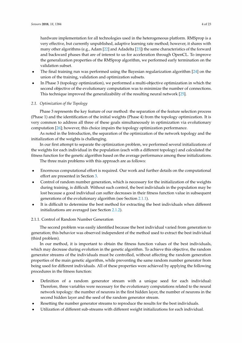
• A fitness function with the goal of obtaining the best fitness function value for the evolutionarycomputation of the initial weights (as in Phase 4); in other words, the execution of a subordinateevolutionary computation for each individual as part of the main evolutionary computation.This alternative is called GATOPOGA or GATOPODE, depending on the evolutionary algorithmused in the second-level evolutionary computation: a genetic algorithm (GA) or differentialevolution (DE) (see Figure 1). This scheme is obtained based on the studies carried out by [27].

• A fitness function with the goal of minimizing the MSE of resilient BP when the initialweights have been established using auto-encoders [28]. This technique is very commonlyused for the non-supervised training of deep neural networks (DNNs). This alternative iscalled GATOPODNN.

A detailed assessment of these three alternatives is outside the scope of this study. However,the computational effort required for each alternative is obvious, as is the need for high flexibility inthe implementation of the individuals for the genetic algorithm.

If we suppose that a population of 100 individuals is considered in the main genetic algorithm,we can assess the number of RMSprop training runs needed in one generation as follows:

• With 50 different initializations, we would need 5000 RMSprop training runs in each generation.• With 500 individuals considered in the second-level evolutionary computation (GA or DE),

we would need 50,000 RMSprop training runs in each generation of the main genetic algorithm.• With an MLP with three layers of weights, we would need 300 RMSprop training runs for two

layers of MLP weights in each generation and 100 RMSprop training runs for three layers of MLPweights in each generation.

GA

DE

RMSPRMSPRMSP

DE

RMSPRMSP RMSP RMSPRMSPRMSP

DE

Topology 2

Host

IW12IW 11 IW 1M IW22IW 21 IW 2M IWN2IWN1 IWNM

Topology 1 Topology N

Figure 1. Structure of Phase 3 for GATOPODE. DE, differential evolution.

3. Heterogeneous Computational Platform

In our implementation, the neural network optimization method introduced in Section 2(specifically, Phase 3 of the method) requires a host processor responsible for the main genetic algorithm,which manages the derivation of the ANN topology.

Sensors 2018, 18, 1384 6 of 23

The number of variables to be handled is only three, and therefore, the size of the population to bemanaged is rather limited. For each individual, a neural network must be trained that consists of twohidden layers with one set of initial weights, in the case of the non-supervised method (GATOPODNN);various random weight initializations (GATOPOMEAN and GATOPOMIN); or initial weights obtainedvia a nested genetic algorithm, in the most complex case (GATOPOGAand GATOPODE).

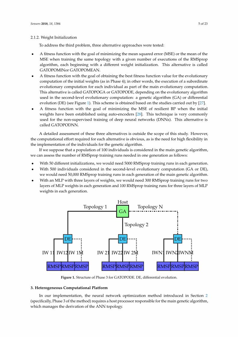
To implement the host processor, we opted for a generalist solution based on a multicore CPUusing Python, enabling us to easily adapt the solution to other platforms to generate experimentalsamples, perform quick implementation comparisons with existing toolboxes for global optimizationmethods and neural network implementations and obtain a straightforward representation of theresults. This generalist host platform had access to a GPU via a graphics board connected to the mainboard. Our study does not focus on this host processor, as it is a very common platform, but theminimum requirements are described. The structure can be seen at the top of Figure 2.

Host CPU Multicore

ARM

FPGA

Nios

NewALU.

ARM

FPGA

Nios

Coproc.

Bus PCIGPU 1

TCP/IP

GPU 2

Bus PCI

FPGA1 FPGASoC4CPU + GPU

FPGA3

Figure 2. Heterogeneous computational platform.

Our main modification to this platform was to add the ability for the host processor toconnect (via simple socket clients) to a set of embedded processors (soft or hard) using FPGAtechnology, thereby providing us with many different system-on-a-chip (SoC) solutions (Figure 2).This modification enabled us to adopt the following alternative implementations of the individuals forthe main genetic algorithm:

• local individuals

– CPU cores– GPU processors

• remote individuals on FPGAs

– FPGA0 soft embedded processor

Sensors 2018, 18, 1384 7 of 23

– FPGA1 soft embedded processor + soft embedded processor with neural instructions– FPGA2 soft embedded processor + programmable coprocessor in software (technological

solution provided in [20])– FPGA3 soft embedded processor + reconfigurable coprocessor

• remote individuals on FPGA-SoCs

– FPGA-SoC0 hard embedded processor– FPGA-SoC1 hard embedded processor + soft embedded processor with neural instructions– FPGA-SoC2 hard embedded processor + programmable coprocessor in software– FPGA-SoC3 hard embedded processor + reconfigurable coprocessor (technological solution

provided in this paper work)

• remote individuals with OpenCL solutions

– FPGA-SoC4 hard embedded processor + reconfigurable kernel– FPGA4 soft embedded processor + reconfigurable kernel– CPU1 + PCI Express GPU kernel– CPU2 + PCI Express FPGA kernel

We started with solutions [20] that were technologically possible based on devices using theAltera Cyclone IV family (remote individuals on FPGAs of type FPGA2) in which the soft processor isALTERA’s NIOS2 microprocessor. It was found that the FPGA-technology-enabled solutions (remoteindividuals on FPGA-SoCs) required the ability to draw on the features provided by devices in theIntel FPGA Cyclone V family, which are common in new devices from other FPGA vendors and thatare essential for understanding the main differences from our previous work from an implementationtechnology point of view:

– Embedded hard cores (Integrated ARM Cortex-A9 MPCore Processor System)– Runtime reconfiguration– Partial reconfiguration– Use of OpenCL solutions and, therefore, quasi-compatible solutions, with others technologies

(CPU-GPU)

There are several precedents for the implementation of neural networks on FPGAs. The workin [29] developed a coprocessor for convolutional neural networks (CNNs) and investigated theacceleration it achieved when applied before other technologies (CPU). The work in [30] presenteda training platform for a reconfigurable topology. The drawback to this application is that it mustre-synthesize the topology each time it is changed and then implement the new topology on theFPGA. Another previous application involved the implementation of a fixed-topology ANN anda BP algorithm for training [31]. The work in [32] proposed a BP algorithm implementation on asoftware-reconfigurable FPGA. Pinjare et al. [33] developed an FPGA accelerator for online training.The work in [34] evaluated their methodology using an FPGA. They were also able to extract the bestperformance density from the FPGA, although they were the only researchers to date to employfloating-point numeric representations in their computations, and the soft embedded processorwas used only to assist with CNN accelerator startup, communication with the host CPU andtime measurement. Their accelerator achieved a 4.79× performance gain over a 16-threaded CNNimplementation on a baseline CPU, with 5.1× less power consumption and a 24.6× energy reduction.

In the majority of these studies, the implementations of ANNs on FPGAs (with online training)have relied on very complex and efficient PEs; however, these implementations present great difficultiesin terms of communication, flexibility and, above all, their adaptability to technological changes.New work such as [35] may represent a change in this sense, in which this lack of flexibility can beovercome; but in general terms, few works are capable of delivering better performance results than

Sensors 2018, 18, 1384 8 of 23

GPUs, unless we move on to those recognizable as binarized neural networks that have a drasticreduction in the resolution of computations performed [36] or by comparison with SoC GPU [37].

The first step in the implementation of individuals on our platform was to resolve the issue ofcommunication with the host for the particular type of algorithm running on the host. Resolving thisissue requires that a portion of the platform that is handling the individuals is used to implement aprocessor for managing a socket server. Therefore, in each of our FPGA-based solutions, there is onemain processor (soft or hard macro) responsible for this task, usually requiring an operating system toassist in socket management.

To address the issue of platform flexibility, we first focused on implementations that allowthe implementation of neural networks with different topologies using an architecture acting as acoprocessor that acquires instructions from the main processor. Therefore, a new task was assigned tothe main processor: compilation of the instructions for the coprocessor. However, we are certain thatin the future, accelerators with finer granularity will be realized on FPGAs (called kernels), which willallow direct compilation based on OpenCL and will be able to be reused in various parts of theexecution of the original algorithm while permitting run-time reconfiguration.

Finally, the issue of ensuring both flexibility and adaptability was resolved by using a designflow based on an OpenCL language that allowed us to reconfigure and compare different technologiesfor enhancing lossless application efficiency in the implementation methodology. The use of theselanguages prepared for a multi-platform compilation currently constitutes one of the lines of greatestproduction in the implementation of deep neural networks associated with CNN networks [38–40].

3.1. Implementation of the Individuals

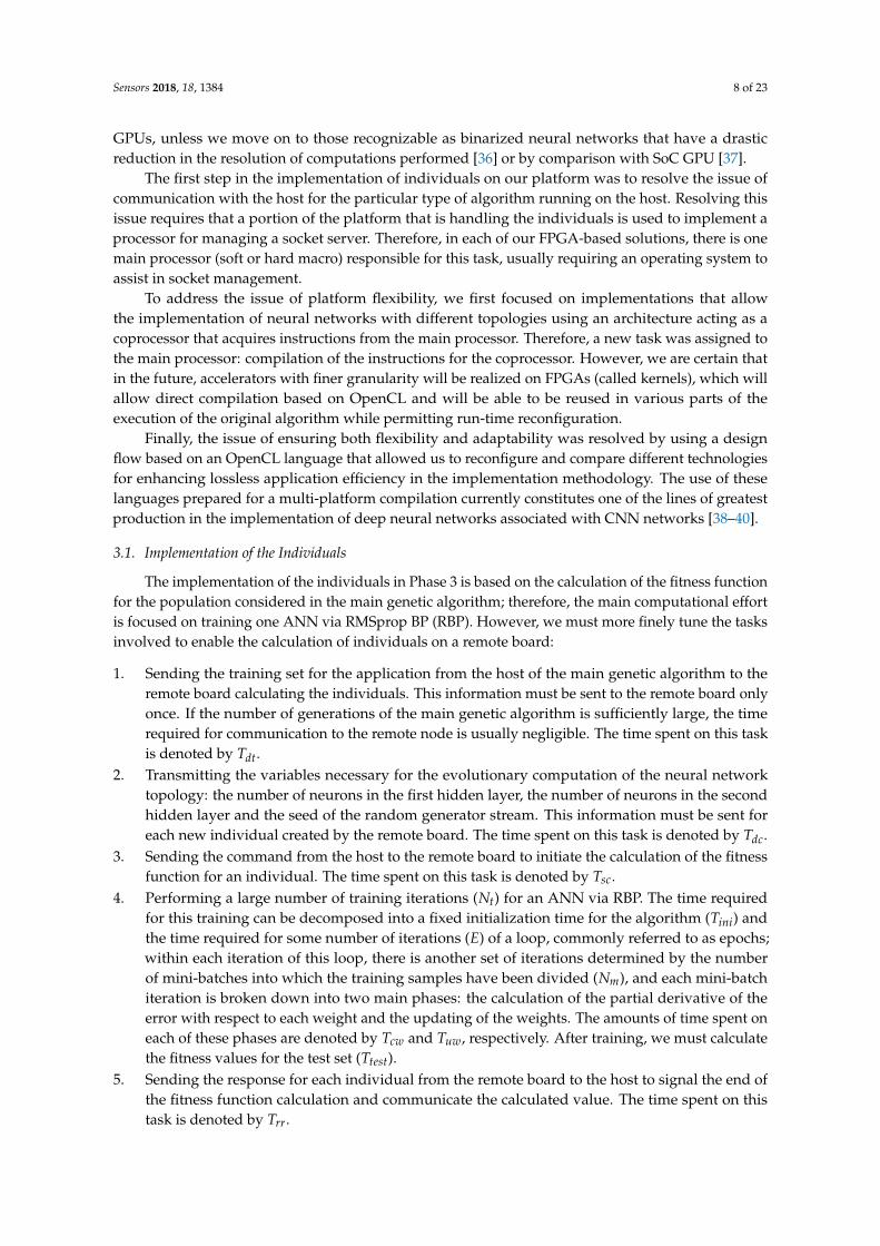
The implementation of the individuals in Phase 3 is based on the calculation of the fitness functionfor the population considered in the main genetic algorithm; therefore, the main computational effortis focused on training one ANN via RMSprop BP (RBP). However, we must more finely tune the tasksinvolved to enable the calculation of individuals on a remote board:

1. Sending the training set for the application from the host of the main genetic algorithm to theremote board calculating the individuals. This information must be sent to the remote board onlyonce. If the number of generations of the main genetic algorithm is sufficiently large, the timerequired for communication to the remote node is usually negligible. The time spent on this taskis denoted by Tdt.

2. Transmitting the variables necessary for the evolutionary computation of the neural networktopology: the number of neurons in the first hidden layer, the number of neurons in the secondhidden layer and the seed of the random generator stream. This information must be sent foreach new individual created by the remote board. The time spent on this task is denoted by Tdc.

3. Sending the command from the host to the remote board to initiate the calculation of the fitnessfunction for an individual. The time spent on this task is denoted by Tsc.

4. Performing a large number of training iterations (Nt) for an ANN via RBP. The time requiredfor this training can be decomposed into a fixed initialization time for the algorithm (Tini) andthe time required for some number of iterations (E) of a loop, commonly referred to as epochs;within each iteration of this loop, there is another set of iterations determined by the numberof mini-batches into which the training samples have been divided (Nm), and each mini-batchiteration is broken down into two main phases: the calculation of the partial derivative of theerror with respect to each weight and the updating of the weights. The amounts of time spent oneach of these phases are denoted by Tcw and Tuw, respectively. After training, we must calculatethe fitness values for the test set (Ttest).

5. Sending the response for each individual from the remote board to the host to signal the end ofthe fitness function calculation and communicate the calculated value. The time spent on thistask is denoted by Trr.

Sensors 2018, 18, 1384 9 of 23

Finally, we have the following time for the execution of G generations of the main geneticalgorithm with a population of P individuals when we use one board for the implementation ofthe individuals:

Tdt + G · P · (Tdc + Nt · (RBP) + Trr) (1)

being:RBP = Tini + E · Nm · (Tcw + Tuw) + Ttest (2)

The remaining time required for optimization via the genetic algorithm is the computation timefor the main processor in our platform (Tmain), which is independent of the type of implementation(local or remote) that is used for the individuals.

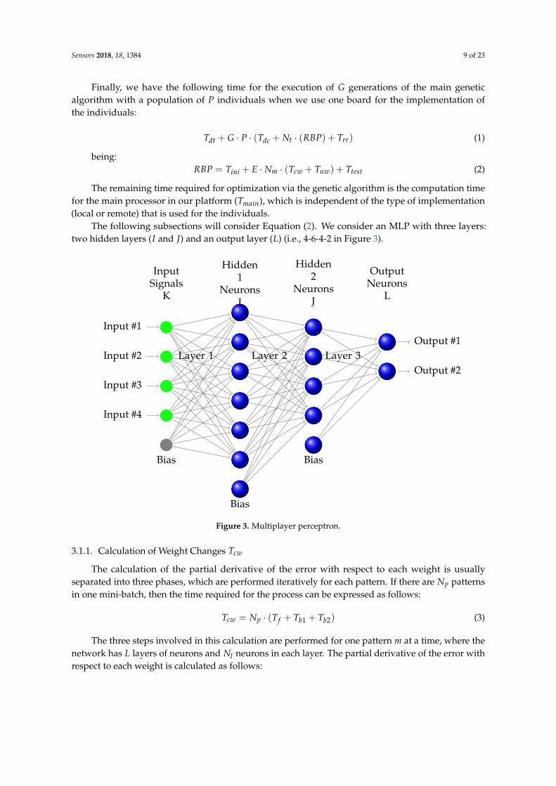
The following subsections will consider Equation (2). We consider an MLP with three layers:two hidden layers (I and J) and an output layer (L) (i.e., 4-6-4-2 in Figure 3).

Input #1

Input #2

Input #3

Input #4

Output #1

Output #2

Hidden1

NeuronsI

Hidden2

NeuronsJ

InputSignals

K

OutputNeurons

L

Bias

Bias

Bias

Layer 1 Layer 2 Layer 3

Figure 3. Multiplayer perceptron.

3.1.1. Calculation of Weight Changes Tcw

The calculation of the partial derivative of the error with respect to each weight is usuallyseparated into three phases, which are performed iteratively for each pattern. If there are Np patternsin one mini-batch, then the time required for the process can be expressed as follows:

Tcw = Np · (Tf + Tb1 + Tb2) (3)

The three steps involved in this calculation are performed for one pattern m at a time, where thenetwork has L layers of neurons and Nl neurons in each layer. The partial derivative of the error withrespect to each weight is calculated as follows:

Sensors 2018, 18, 1384 10 of 23

– Tf : Forward step. Apply the pattern yKi to the input layer and propagate the signal forward

through the network until the final outputs yLi have been calculated for each i (the neuron index)

and l (the layer index).

uli =

Nl−1

∑j=0

wlijy

l−1j (4)

yli = f (ul

i) (5)

y′li = f ′(uli) (6)

1 ≤ i ≤ Nl , 1 ≤ l ≤ L

where y is an activation, w is a weight and f is a non-linear function.

– Tb1: Backward Step 1. Compute the δ values for the output layer L and for the preceding layersby propagating the errors backwards using:

δLj = f ′(uL

j )(ti − yi) (7)

θl−1i =

Nl∑i=1

wijδli (8)

δl−1j = f ′(ul−1

j )θl−1i (9)

1 ≤ i ≤ Nl , 2 ≤ l ≤ L

where δ is the error term, t is the target and f ′ is the derivative of the function f .

– Tb2: Backward Step 2. When we obtain the delta errors in Backward Step 1, we can simultaneouslyobtain the accumulated partial derivative of the error with respect to each weight as follows:

e = 1/2Nl∑i=1

(ti − yLi )

2(10)

m ∂e∂wl

ij= δl

i yl−1j (11)

mcwlij =

m−1cwlij +

m ∂e∂wl

ij(12)

1 ≤ i ≤ Nl , 1 ≤ l ≤ L

where cw is the accumulated direction of the error gradient. Once we have finished processing allof the patterns, the accumulated result will be:

cwlij =

∂E∂wl

ij(13)

E =1

2Np

Np

∑m=1

Nl∑i=1

(ti − yLi )

2(14)

1 ≤ l ≤ L

All of the elements needed in Backward Step 2 are provided at the same time as the elementsnecessary for Backward Step 1. Therefore, it is possible to perform these two final steps simultaneouslyduring the execution of each layer. This action reduces the number of steps to two: a forward step and

Sensors 2018, 18, 1384 11 of 23

a backward step. However, in the OpenCL implementation, it is necessary to clearly differentiate thesesteps and only begin Backward Step 2 when Backward Step 1 has completely finished.

3.1.2. Update of Weights Tuw

The updating of the ANN weights requires the realization of all of the weights of the ANN wheneach epoch has finished.

wij(t+1) = wji

(t) + ∆wij(t) (15)

∆wij(t)=

(∂E

∂wij

)(t)

·∆(t)

ij√r(t)ij

(16)

r(t)ij = (1− γ) ·

( ∂E∂wij

)2(t)

+ γ · r(t−1)ij (17)

∆ij(t)=

(1 + η+)·∆ij(t−1), if

(∂E

∂wij

)(t−1)∗(

∂E∂wij

)(t)> 0

(1− η−)·∆ij(t−1), if

(∂E

∂wij

)(t−1)∗(

∂E∂wij

)(t)< 0

∆ij(t−1), else

where 0 < η− < 1 < η+

(18)

Once the equations necessary for the execution of a neuronal network training in an individual(what we have called RBP) have been broken down, it is necessary to look at the following Algorithm 1.

In this algorithm, we place in each execution line:

– to the right, the equations involved as listed above and– to the left, an identification that allows us to understand which of these operations are

implemented by our OpenCL kernel in the three main versions developed and that now wewill detail.

As we advance in the three versions, we will observe how our kernel will assume more lines ofexecution of our algorithm, which will result in a greater complexity of the OpenCL developed inexchange for a clear decrease in the data communications between the main microprocessor (ARM)and the kernel (FPGA) in each individual.

3.2. Version 1: Algorithm with Kernel of Type Matrix Multiplication

To implement Algorithm 1 in OpenCL, our main candidates for the kernels are Lines 1, 2, 3, 4, 5,6, 7 and 8 of Algorithm 1. Each of these kernels would have a similar structure based on matrix-matrixmultiplication and on the path dependence that exists between them. Therefore, a better solutionwould be to implement a single kernel and reuse it eight times in each iteration. With this approach,we would use the same kernel 8 · E times in our algorithm.

Equation (19) shows the matrix-matrix multiplications necessary for the forward phase.Equation (20) shows the matrix-matrix multiplications necessary for Backward Phase 1. Equation (21)shows the matrix-matrix multiplications necessary for Backward Phase 2. In each matrix-matrixmultiplication, the size of the matrices must be modified, and thus, our OpenCL implementation mustpermit the modification of these parameters. Note that it is necessary to transfer new input matricesand read new matrix output via memory buffers every time the kernel is reused.

Sensors 2018, 18, 1384 12 of 23

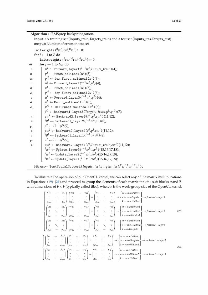
Algorithm 1: RMSprop backpropagation.input :A training set (Inputs_train,Targets_train) and a test set (Inputs_tets,Targets_test)output :Number of errors in test set

Initweights (0wI ,0wJ ,0wL)← 0;for i← 1 to E do

Initcweights (0cwI ,0cwJ ,0cwL)← 0;Mb for j← 1 to Nm do

1 uI ← Forward_layer1(i−1wI ,Inputs_train)(4);th yI ← Funct_nolineal(uI)(5);dt y′I ← der_Funct_nolineal(uI)(6);2 uJ ← Forward_layer2(i−1wJ ,yI)(4);

th yJ ← Funct_nolineal(uJ)(5);dt y′J ← der_Funct_nolineal(uJ)(6);3 uL ← Forward_layer3(i−1wL,yJ)(4);

th yL ← Funct_nolineal(uL)(5);dt y′L ← der_Funct_nolineal(uL)(6);

δL ← Backward1_layer3(Targets_train,yL,y′L)(7);4 cwL ← Backward2_layer3(δL,yJ ,cwL)(11,12);5 jθ J ← Backward1_layer2(i−1wL,δL)(8);

pr δJ ← jθ J · y′J(9);6 cwJ ← Backward2_layer2(δJ ,yI ,cwJ)(11,12);7 jθ I ← Backward1_layer1(i−1wJ ,δJ)(8);

pr δI ← jθ I · y′I(9);8 cwI ← Backward2_layer1(δI ,Inputs_train,cwI)(11,12);

iwL ← Update_layer3(i−1wL,cwL)(15,16,17,18);iwJ ← Update_layer2(i−1wJ ,cwJ)(15,16,17,18);iwI ← Update_layer1(i−1wI ,cwI)(15,16,17,18);

Fitness← TestNeuralNetwork(Inputs_test,Targets_test,EwI ,EwJ ,EwL);

To illustrate the operation of our OpenCL kernel, we can select any of the matrix multiplicationsin Equations (19)–(21) and proceed to group the elements of each matrix into the sub-blocks Aand Bwith dimensions of b× b (typically called tiles), where b is the work-group size of the OpenCL kernel.

I11 . . . I1n

.... . .

...Im1 · · · Imn

w11 . . . wk1

.... . .

...w1n · · · wkn

=

u11 . . . u1k

.... . .

...um1 · · · umk

→

m = numPattern

n = numInputs

k = numHidden1

→ f orward− layer1

y11 . . . y1n

.... . .

...ym1 · · · ymn

w11 . . . wk1

.... . .

...w1n · · · wkn

=

u11 . . . u1k

.... . .

...um1 · · · umk

→

m = numPattern

n = numHidden1

k = numHidden2


y11 . . . y1n

.... . .

...ym1 · · · ymn

w11 . . . wk1

.... . .

...w1n · · · wkn

=

u11 . . . u1k

.... . .

...um1 · · · umk

→

m = numPattern

n = numHidden2

k = nuOutputs


(19)

δ11 . . . δ1n

.... . .

...δm1 · · · δmn

w11 . . . w1k

.... . .

...wn1 · · · wnk

=

θ11 . . . θ1k

.... . .

...θm1 · · · θmk

→

m = numPattern

n = numOutputs

k = numHidden2

→ backward1− layer2

δ11 . . . δ1n

.... . .

...δm1 · · · δmn

w11 . . . w1k

.... . .

...wn1 · · · wnk

=

θ11 . . . θ1k

.... . .

...θm1 · · · θmk

→

m = numPattern

n = numHidden2

k = numHidden1


(20)

Sensors 2018, 18, 1384 13 of 23

δ11 . . . δ1n

.... . .

...δm1 · · · δmn

y11 . . . y1k

.... . .

...yn1 · · · ynk

=

cw11 . . . cw1k

.... . .

...cwm1 · · · cwmk

→

m = numOutputs

n = numPattern

k = numHidden2


δ11 . . . δ1n

.... . .

...δm1 · · · δmn

y11 . . . y1k

.... . .

...yn1 · · · ynk

=

cw11 . . . cw1k

.... . .

...cwm1 · · · cwmk

→

m = numHidden2

n = numPattern

k = numHidden1


δ11 . . . δ1n

.... . .

...δm1 · · · δmn

y11 . . . y1k

.... . .

...yn1 · · · ynk

=

cw11 . . . cw1k

.... . .

...cwm1 · · · cwmk

→

m = numHidden1

n = numPattern

k = numInputs


(21)

OpenCL requires that the number of work-groups is chosen such that the size of theNDRangeindex space is evenly divided in each dimension. Therefore, it is necessary for our BPalgorithm to guarantee this property of the matrix dimensions in Equations (19)–(21).

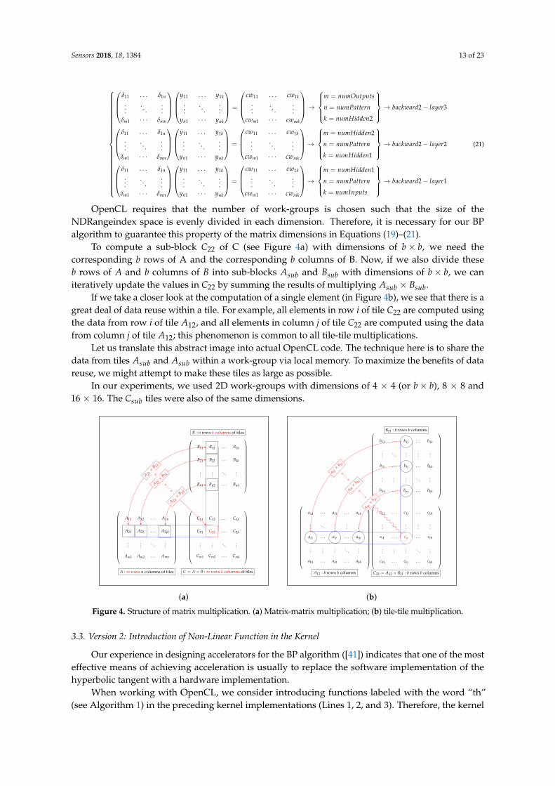
To compute a sub-block C22 of C (see Figure 4a) with dimensions of b× b, we need thecorresponding b rows of A and the corresponding b columns of B. Now, if we also divide theseb rows of A and b columns of B into sub-blocks Asub and Bsub with dimensions of b× b, we caniteratively update the values in C22 by summing the results of multiplying Asub × Bsub.

If we take a closer look at the computation of a single element (in Figure 4b), we see that there is agreat deal of data reuse within a tile. For example, all elements in row i of tile C22 are computed usingthe data from row i of tile A12, and all elements in column j of tile C22 are computed using the datafrom column j of tile A12; this phenomenon is common to all tile-tile multiplications.

Let us translate this abstract image into actual OpenCL code. The technique here is to share thedata from tiles Asub and Asub within a work-group via local memory. To maximize the benefits of datareuse, we might attempt to make these tiles as large as possible.

In our experiments, we used 2D work-groups with dimensions of 4 × 4 (or b× b), 8 × 8 and16 × 16. The Csub tiles were also of the same dimensions.

A11 A12 . . . A1n

A21 A22 . . . A2p;

......

. . ....

Am1 Am2 . . . Amn

A : m rows n columns of tiles

B11 B12 . . . B1k

B21 B22 . . . B2k

......

. . ....

Bn1 Bp2 . . . Bnk

B : n rows k columns of tiles

C11 C12 . . . C1k

C21 C22 . . . C2k

......

. . ....

Cm1 Cm2 . . . Cmk

A 21×

B 12

A 22×

B 22

A 2p×

B p2

+

+ . . .+

C = A× B : m rows k columns of tiles

(a)

a11 . . . a1t . . . a1b

.... . .

......

...

ai1 . . . ait . . . aib

......

.... . .

...

ab1 . . . abt . . . abb

A12 : b rows b columns

b11 . . . b1j . . . b1b

.... . .

......

...

bt1 . . . btj . . . bkb

......

.... . .

...

bb1 . . . bnj . . . bbb

B21 : b rows b columns

c11 . . . c1j . . . c1b

.... . .

......

...

ci1 . . . cij . . . cib

......

.... . .

...

cb1 . . . cbj . . . cbb

C22 = A12 × B21 : b rows b columns

a i1×

b 1j

a ik×

b kj

a ip×

b pj

+ . . .+

+ . . .+

(b)

Figure 4. Structure of matrix multiplication. (a) Matrix-matrix multiplication; (b) tile-tile multiplication.

3.3. Version 2: Introduction of Non-Linear Function in the Kernel

Our experience in designing accelerators for the BP algorithm ([41]) indicates that one of the mosteffective means of achieving acceleration is usually to replace the software implementation of thehyperbolic tangent with a hardware implementation.

When working with OpenCL, we consider introducing functions labeled with the word “th”(see Algorithm 1) in the preceding kernel implementations (Lines 1, 2, and 3). Therefore, the kernel

Sensors 2018, 18, 1384 14 of 23

must support non-linear hyperbolic tangent operations in calls to the kernel belonging to the “forward”phase of the BP algorithm.

If we introduce the hyperbolic tangent in our OpenCL file, the definition of tanh(x) is sinh(x)/cosh(x),which is equivalent to the three formulae given in Equation (22) below.

(ex − e−x)/(ex + e−x)

(1− (2/(e2x + 1))

(e2x − 1)/(e2x + 1)

(22)

The results for this type of solution show that the cost of FPGA hardware resources is high,and the benefits achieved are not decisive (see the results for raw tanh OpenCL in Table 1).

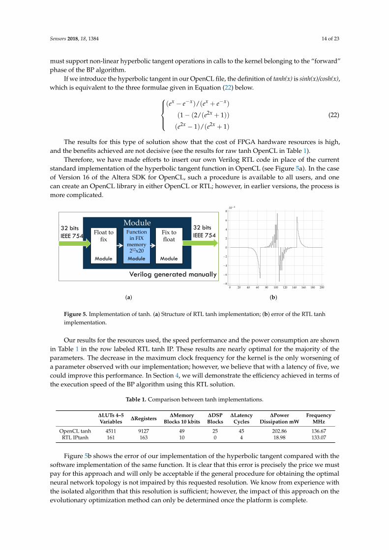
Therefore, we have made efforts to insert our own Verilog RTL code in place of the currentstandard implementation of the hyperbolic tangent function in OpenCL (see Figure 5a). In the caseof Version 16 of the Altera SDK for OpenCL, such a procedure is available to all users, and onecan create an OpenCL library in either OpenCL or RTL; however, in earlier versions, the process ismore complicated.

Module32 bits

IEEE 754Float to

fix

Functionin FIX

memory212x20

Fix to float

32 bits

IEEE 754

Verilog generated manually

Module ModuleModule

(a)

0 20 40 60 80 100 120 140 160 180 200−8

−6

−4

−2

0

2

4

6

8·10−4

(b)

Figure 5. Implementation of tanh. (a) Structure of RTL tanh implementation; (b) error of the RTL tanhimplementation.

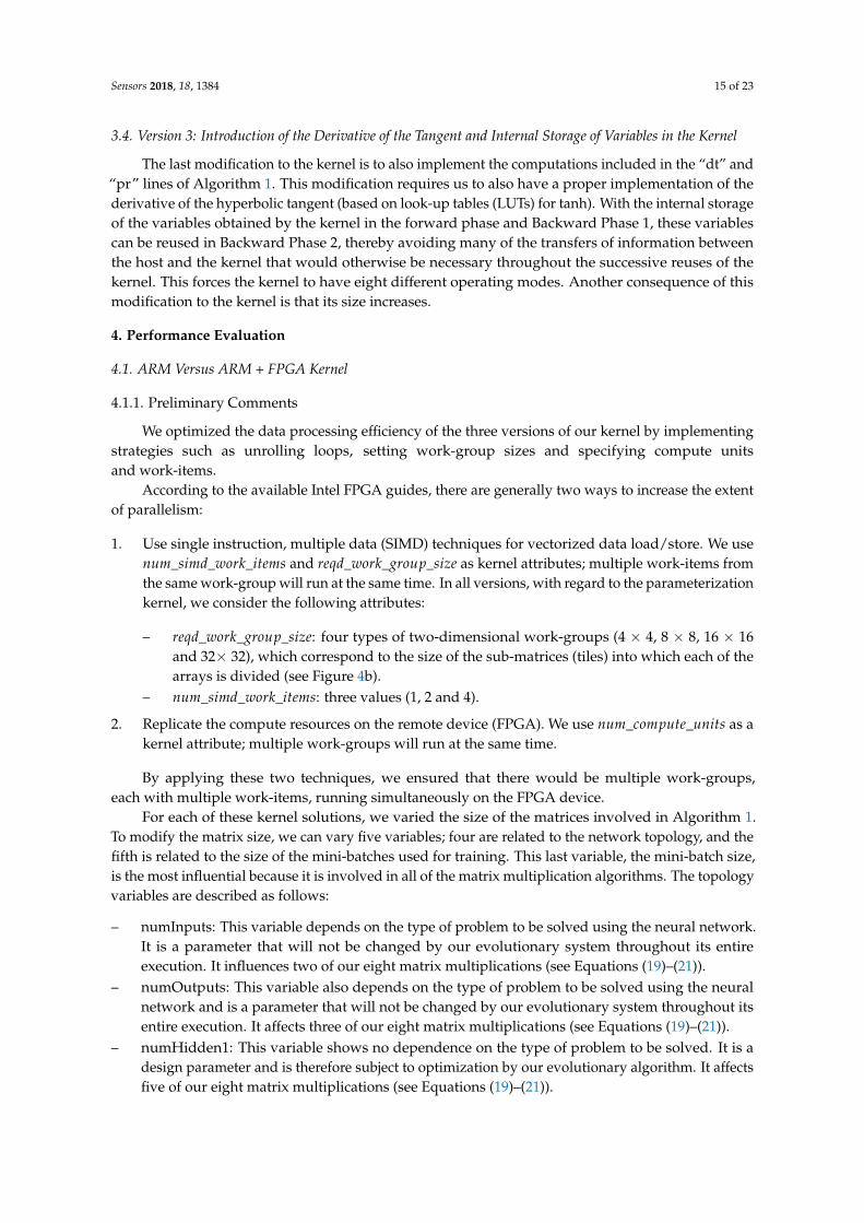
Our results for the resources used, the speed performance and the power consumption are shownin Table 1 in the row labeled RTL tanh IP. These results are nearly optimal for the majority of theparameters. The decrease in the maximum clock frequency for the kernel is the only worsening ofa parameter observed with our implementation; however, we believe that with a latency of five, wecould improve this performance. In Section 4, we will demonstrate the efficiency achieved in terms ofthe execution speed of the BP algorithm using this RTL solution.

Table 1. Comparison between tanh implementations.

∆LUTs 4–5∆Registers ∆Memory ∆DSP ∆Latency ∆Power Frequency

Variables Blocks 10 kbits Blocks Cycles Dissipation mW MHz

OpenCL tanh 4511 9127 49 25 45 202.86 136.67RTL IPtanh 161 163 10 0 4 18.98 133.07

Figure 5b shows the error of our implementation of the hyperbolic tangent compared with thesoftware implementation of the same function. It is clear that this error is precisely the price we mustpay for this approach and will only be acceptable if the general procedure for obtaining the optimalneural network topology is not impaired by this requested resolution. We know from experience withthe isolated algorithm that this resolution is sufficient; however, the impact of this approach on theevolutionary optimization method can only be determined once the platform is complete.

Sensors 2018, 18, 1384 15 of 23

3.4. Version 3: Introduction of the Derivative of the Tangent and Internal Storage of Variables in the Kernel

The last modification to the kernel is to also implement the computations included in the “dt” and“pr” lines of Algorithm 1. This modification requires us to also have a proper implementation of thederivative of the hyperbolic tangent (based on look-up tables (LUTs) for tanh). With the internal storageof the variables obtained by the kernel in the forward phase and Backward Phase 1, these variablescan be reused in Backward Phase 2, thereby avoiding many of the transfers of information betweenthe host and the kernel that would otherwise be necessary throughout the successive reuses of thekernel. This forces the kernel to have eight different operating modes. Another consequence of thismodification to the kernel is that its size increases.

4. Performance Evaluation

4.1. ARM Versus ARM + FPGA Kernel

4.1.1. Preliminary Comments

We optimized the data processing efficiency of the three versions of our kernel by implementingstrategies such as unrolling loops, setting work-group sizes and specifying compute unitsand work-items.

According to the available Intel FPGA guides, there are generally two ways to increase the extentof parallelism:

1. Use single instruction, multiple data (SIMD) techniques for vectorized data load/store. We usenum_simd_work_items and reqd_work_group_size as kernel attributes; multiple work-items fromthe same work-group will run at the same time. In all versions, with regard to the parameterizationkernel, we consider the following attributes:

– reqd_work_group_size: four types of two-dimensional work-groups (4 × 4, 8 × 8, 16 × 16and 32× 32), which correspond to the size of the sub-matrices (tiles) into which each of thearrays is divided (see Figure 4b).

– num_simd_work_items: three values (1, 2 and 4).

2. Replicate the compute resources on the remote device (FPGA). We use num_compute_units as akernel attribute; multiple work-groups will run at the same time.

By applying these two techniques, we ensured that there would be multiple work-groups,each with multiple work-items, running simultaneously on the FPGA device.

For each of these kernel solutions, we varied the size of the matrices involved in Algorithm 1.To modify the matrix size, we can vary five variables; four are related to the network topology, and thefifth is related to the size of the mini-batches used for training. This last variable, the mini-batch size,is the most influential because it is involved in all of the matrix multiplication algorithms. The topologyvariables are described as follows:

– numInputs: This variable depends on the type of problem to be solved using the neural network.It is a parameter that will not be changed by our evolutionary system throughout its entireexecution. It influences two of our eight matrix multiplications (see Equations (19)–(21)).

– numOutputs: This variable also depends on the type of problem to be solved using the neuralnetwork and is a parameter that will not be changed by our evolutionary system throughout itsentire execution. It affects three of our eight matrix multiplications (see Equations (19)–(21)).

– numHidden1: This variable shows no dependence on the type of problem to be solved. It is adesign parameter and is therefore subject to optimization by our evolutionary algorithm. It affectsfive of our eight matrix multiplications (see Equations (19)–(21)).

Sensors 2018, 18, 1384 16 of 23

– numHidden2: This variable also shows no dependence on the type of problem to be solved; itis also a design parameter and therefore subject to optimization by our evolutionary algorithm.It affects six of our eight matrix multiplications (see Equations (19)–(21)).

Based on this analysis, we opted to maintain our study settings for four of the five variablesin each test, and we individually varied our hardware solutions (mentioned above), the number ofneurons in the first hidden layer, the number of neurons in the second hidden layer and the number ofpatterns per mini-batch.

In each test, only one variable was changed, and the remaining values were set as follows:numPatterns: 65,536 numInputs: 78 numHidden1: 256 numHidden2: 256 numOutputs: 10.

4.1.2. Analysis of Hardware Results

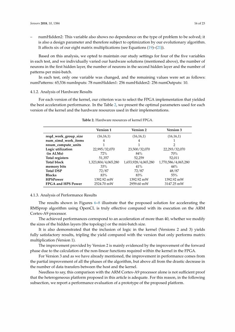
For each version of the kernel, our criterion was to select the FPGA implementation that yieldedthe best acceleration performance. In the Table 2, we present the optimal parameters used for eachversion of the kernel and the hardware resources used in their implementations.

Table 2. Hardware resources of kernel FPGA.

Version 1 Version 2 Version 3

reqd_work_group_size (16,16,1) (16,16,1) (16,16,1)num_simd_work_items 4 4 1nnum_compute_units 1 1 2Logic utilization 22,995/32,070 23,500/32,070 22,293/32,070(in ALMs) 72% 84% 70%Total registers 51,357 52,259 52,011Total block 1,323,804/4,065,280 1,653,928/4,065,280 1,770,586/4,065,280memory bits 33% 41% 44%Total DSP 72/87 72/87 48/87Blocks 83% 83% 55%HPSPower 1392.92 mW 1392.92 mW 1392.92 mWFPGA and HPS Power 2524.70 mW 2959.60 mW 3147.25 mW

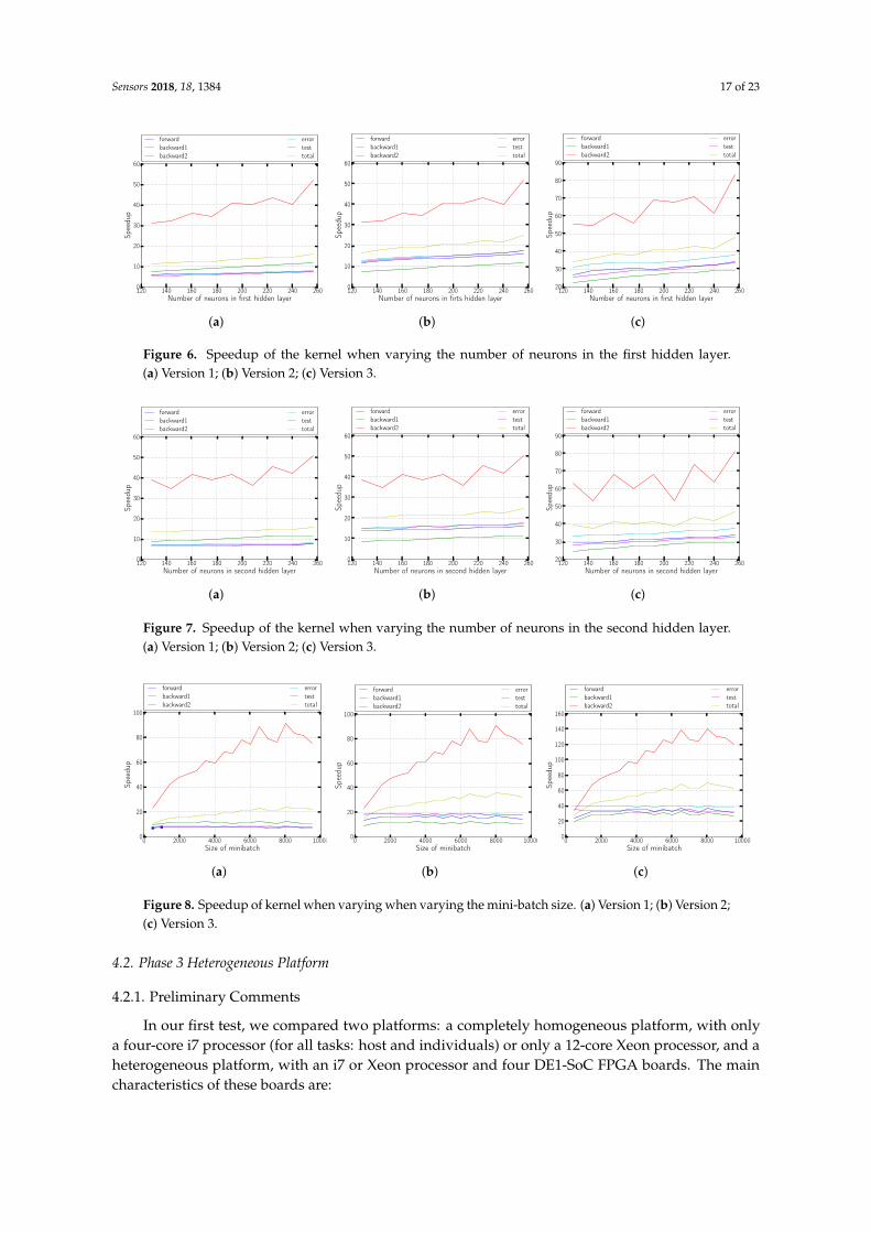
4.1.3. Analysis of Performance Results

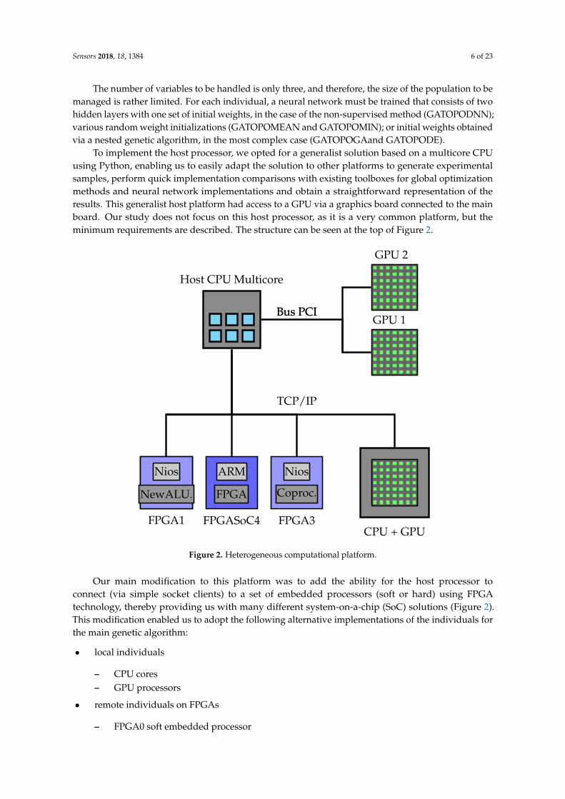
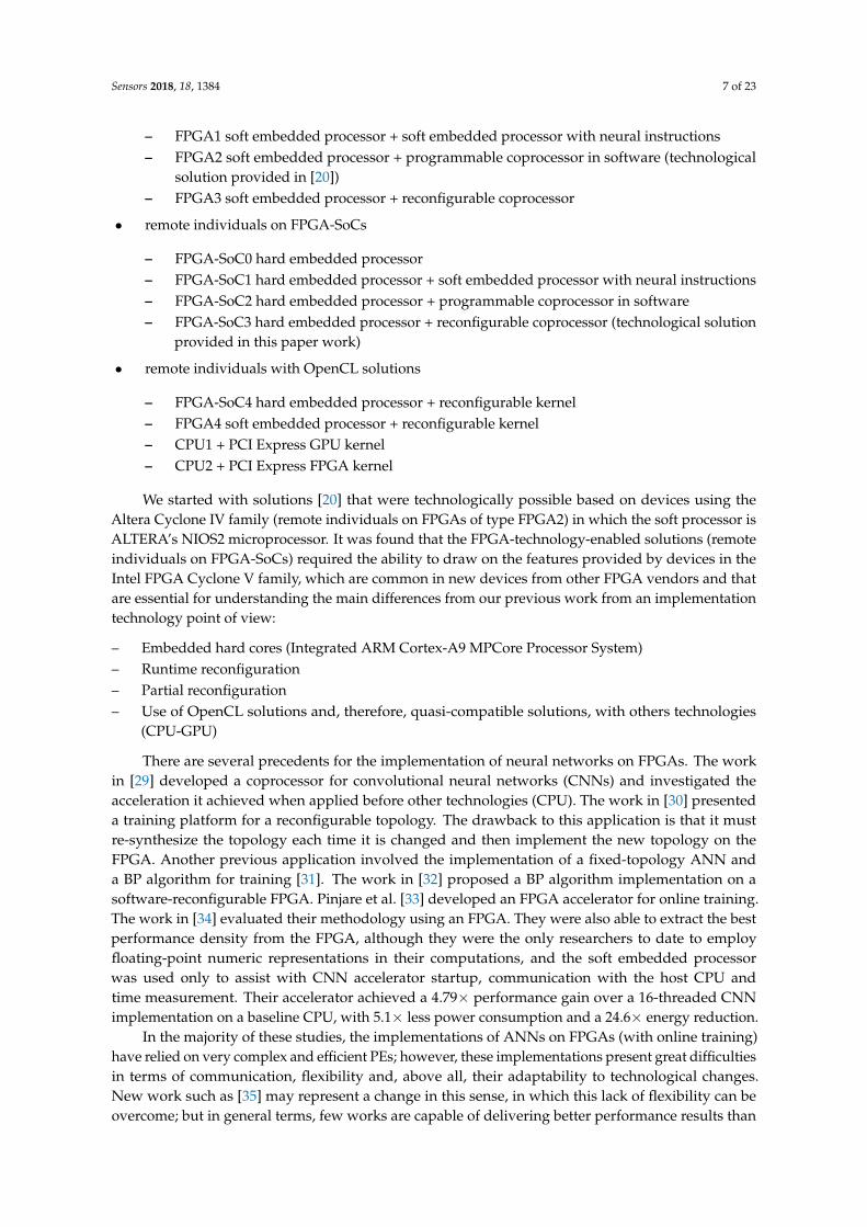
The results shown in Figures 6–8 illustrate that the proposed solution for accelerating theRMSprop algorithm using OpenCL is truly effective compared with its execution on the ARMCortex-A9 processor.

The achieved performances correspond to an acceleration of more than 40, whether we modifythe sizes of the hidden layers (the topology) or the mini-batch size.

It is also demonstrated that the inclusion of logic in the kernel (Versions 2 and 3) yieldsfully satisfactory results, tripling the yield compared with the version that only performs matrixmultiplication (Version 1).

The improvement provided by Version 2 is mainly evidenced by the improvement of the forwardphase due to the calculation of the non-linear functions required within the kernel in the FPGA.

For Version 3 and as we have already mentioned, the improvement in performance comes fromthe partial improvement of all the phases of the algorithm, but above all from the drastic decrease inthe number of data transfers between the host and the kernel.

Needless to say, this comparison with the ARM Cortex-A9 processor alone is not sufficient proofthat the heterogeneous platform proposed in this article is adequate. For this reason, in the followingsubsection, we report a performance evaluation of a prototype of the proposed platform.

Sensors 2018, 18, 1384 17 of 23Sensors 2018, 18, x 17 of 23

120 140 160 180 200 220 240 260Number of neurons in first hidden layer

0

10

20

30

40

50

60

Speedu

p

forwardbackward1backward2

errortesttotal

(a)

120 140 160 180 200 220 240 260Number of neurons in firts hidden layer

0

10

20

30

40

50

60

Speedu

p


errortesttotal

(b)


20

30

40

50

60

70

80

90

Speedu

p


errortesttotal

(c)

Figure 6. Speedup of kernel when varying the number of neurons in the first hidden layer. (a) version 1;(b) version 2; (c) version 3.

120 140 160 180 200 220 240 260Number of neurons in second hidden layer

0

10

20

30

40

50

60

Speedu

p


errortesttotal

(a)


0

10

20

30

40

50

60

Speedu

p


errortesttotal

(b)


20

30

40

50

60

70

80

90

Speedu

p


errortesttotal

(c)

Figure 7. Speedup of kernel when varying the number of neurons in the second hidden layer.(a) version 1; (b) version 2; (c) version 3.

0 2000 4000 6000 8000 10000Size of minibatch

0

20

40

60

80

100

Speedu

p


errortesttotal

(a)


0

20

40

60

80

100

Speedu

p


errortesttotal

(b)


0

20

40

60

80

100

120

140

160

Speedu

p


errortesttotal

(c)

Figure 8. Speedup of kernel when varying when varying the minibatch size. (a) version 1; (b version 2;(c) version 3.

4.2. Phase 3 Heterogeneous Platform


In our first test, we compared two platforms: a completely homogeneous platform, with onlya 4-core i7 processor (for all tasks: host and individuals) or only a 12-core Xeon processor, and aheterogeneous platform, with an i7 or Xeon processor and 4 DE1-SoC FPGA boards. The maincharacteristics of these boards are:

Figure 6. Speedup of the kernel when varying the number of neurons in the first hidden layer.(a) Version 1; (b) Version 2; (c) Version 3.

Sensors 2018, 18, x 17 of 23


0

10

20

30

40

50

60

Speedu

pforwardbackward1backward2

errortesttotal

(a)


0

10

20

30

40

50

60

Speedu

p


errortesttotal

(b)


20

30

40

50

60

70

80

90

Speedu

p


errortesttotal

(c)



0

10

20

30

40

50

60

Speedu

p


errortesttotal

(a)


0

10

20

30

40

50

60

Speedu

p


errortesttotal

(b)


20

30

40

50

60

70

80

90

Speedu

p


errortesttotal

(c)



0

20

40

60

80

100

Speedu

p


errortesttotal

(a)


0

20

40

60

80

100

Speedu

p


errortesttotal

(b)


0

20

40

60

80

100

120

140

160

Speedu

p


errortesttotal

(c)





Figure 7. Speedup of the kernel when varying the number of neurons in the second hidden layer.(a) Version 1; (b) Version 2; (c) Version 3.

Sensors 2018, 18, x 17 of 23


0

10

20

30

40

50

60Sp

eedu

p


errortesttotal

(a)


0

10

20

30

40

50

60

Speedu

p


errortesttotal

(b)


20

30

40

50

60

70

80

90

Speedu

p


errortesttotal

(c)



0

10

20

30

40

50

60

Speedu

p


errortesttotal

(a)


0

10

20

30

40

50

60

Speedu

p


errortesttotal

(b)


20

30

40

50

60

70

80

90

Speedu

p


errortesttotal

(c)



0

20

40

60

80

100

Speedu

p


errortesttotal

(a)


0

20

40

60

80

100

Speedu

p


errortesttotal

(b)


0

20

40

60

80

100

120

140

160

Speedu

p


errortesttotal

(c)





Figure 8. Speedup of kernel when varying when varying the mini-batch size. (a) Version 1; (b) Version 2;(c) Version 3.



In our first test, we compared two platforms: a completely homogeneous platform, with onlya four-core i7 processor (for all tasks: host and individuals) or only a 12-core Xeon processor, and aheterogeneous platform, with an i7 or Xeon processor and four DE1-SoC FPGA boards. The maincharacteristics of these boards are:

Sensors 2018, 18, 1384 18 of 23

– FPGA device:

– Cyclone V SoC 5CSEMA5F31C6 Device– Dual-core ARM Cortex-A9 (HPS)– 85 K programmable logic elements– 4450 Kbits embedded memory– 6 fractional PLLs– 2 hard memory controllers.

– Memory device:

– 64-MB (32 M × 16) SDRAM on FPGA– 1-GB (2 × 256 M × 16) DDR3 SDRAM on HPS and shared with FPGA. OpenCL kernels

access this shared physical memory through direct connection to the HPS DDR hardmemory controller.

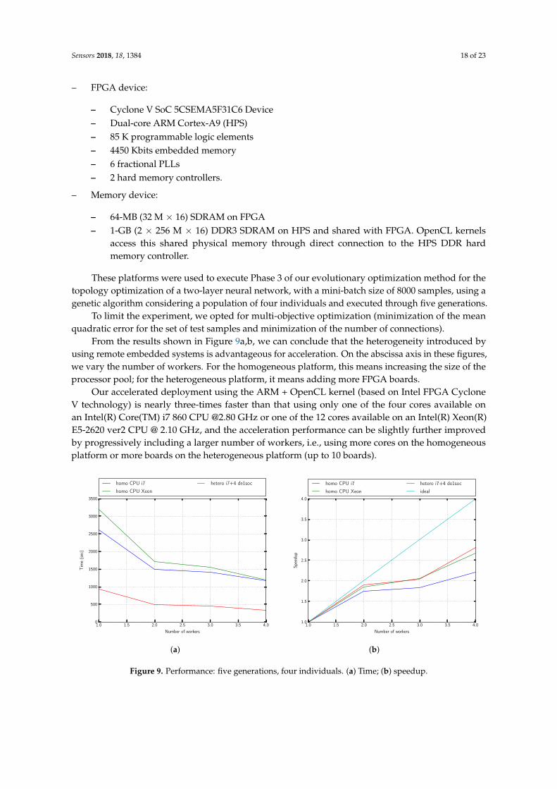
These platforms were used to execute Phase 3 of our evolutionary optimization method for thetopology optimization of a two-layer neural network, with a mini-batch size of 8000 samples, using agenetic algorithm considering a population of four individuals and executed through five generations.

To limit the experiment, we opted for multi-objective optimization (minimization of the meanquadratic error for the set of test samples and minimization of the number of connections).

From the results shown in Figure 9a,b, we can conclude that the heterogeneity introduced byusing remote embedded systems is advantageous for acceleration. On the abscissa axis in these figures,we vary the number of workers. For the homogeneous platform, this means increasing the size of theprocessor pool; for the heterogeneous platform, it means adding more FPGA boards.

Our accelerated deployment using the ARM + OpenCL kernel (based on Intel FPGA CycloneV technology) is nearly three-times faster than that using only one of the four cores available onan Intel(R) Core(TM) i7 860 CPU @2.80 GHz or one of the 12 cores available on an Intel(R) Xeon(R)E5-2620 ver2 CPU @ 2.10 GHz, and the acceleration performance can be slightly further improvedby progressively including a larger number of workers, i.e., using more cores on the homogeneousplatform or more boards on the heterogeneous platform (up to 10 boards).

Sensors 2018, 18, x 18 of 23

– FPGA Device:

– Cyclone V SoC 5CSEMA5F31C6 Device– Dual-core ARM Cortex-A9 (HPS)– 85K Programmable Logic Elements– 4,450 Kbits embedded memory– 6 Fractional PLLs– 2 Hard Memory Controllers.

– Memory Device:

– 64MB (32Mx16) SDRAM on FPGA– 1GB (2x256Mx16) DDR3 SDRAM on HPS and shared with FPGA. OpenCL kernels access this

shared physical memory through direct connection to the HPS DDR hard memory controller.

These platforms were used to execute phase 3 of our evolutionary optimization method for thetopology optimization of a 2-layer neural network, with a minibatch size of 8000 samples, using agenetic algorithm considering a population of 4 individuals and executed through 5 generations.

To limit the experiment, we opted for multi-objective optimization (minimization of the meanquadratic error for the set of test samples and minimization of the number of connections).

From the results shown in Figure 9a,b, we can conclude that the heterogeneity introduced byusing remote embedded systems is advantageous for acceleration. On the abscissa axis in these figures,we vary the number of workers. For the homogeneous platform, this means increasing the size of theprocessor pool; for the heterogeneous platform, it means adding more FPGA boards.

Our accelerated deployment using the ARM+OpenCL kernel (based on Intel FPGA Cyclone Vtechnology) is nearly 3 times faster than that using only one of the 4 cores available on an Intel(R)Core(TM) i7 860 CPU @ 2.80 GHz or one of the 12 cores available on an Intel(R) Xeon(R) E5-2620 ver2CPU @ 2.10 GHz, and the acceleration performance can be slightly further improved by progressivelyincluding a larger number of workers, i.e., using more cores on the homogeneous platform or moreboards on the heterogeneous platform (up to 10 boards).

1.0 1.5 2.0 2.5 3.0 3.5 4.0Number of workers

0

500

1000

1500

2000

2500

3000

3500

Tim

e(s

ec)

homo CPU i7homo CPU Xeon

hetero i7+4 de1soc

(a)

1.0 1.5 2.0 2.5 3.0 3.5 4.0Number of workers

1.0

1.5

2.0

2.5

3.0

3.5

4.0

Spee

dup

homo CPU i7homo CPU Xeon

hetero i7+4 de1socideal

(b)

Figure 9. Performance: 5 generations, 4 individuals. (a) Time; (b) Speedup.Figure 9. Performance: five generations, four individuals. (a) Time; (b) speedup.

Sensors 2018, 18, 1384 19 of 23

4.2.2. Performance Efficiency

In our second test, we extended the utilization of the heterogeneity of the platform to theimplementation of individuals, for which one also can use exclusively the cores of the host machine orcan include the use of remote FPGA boards.

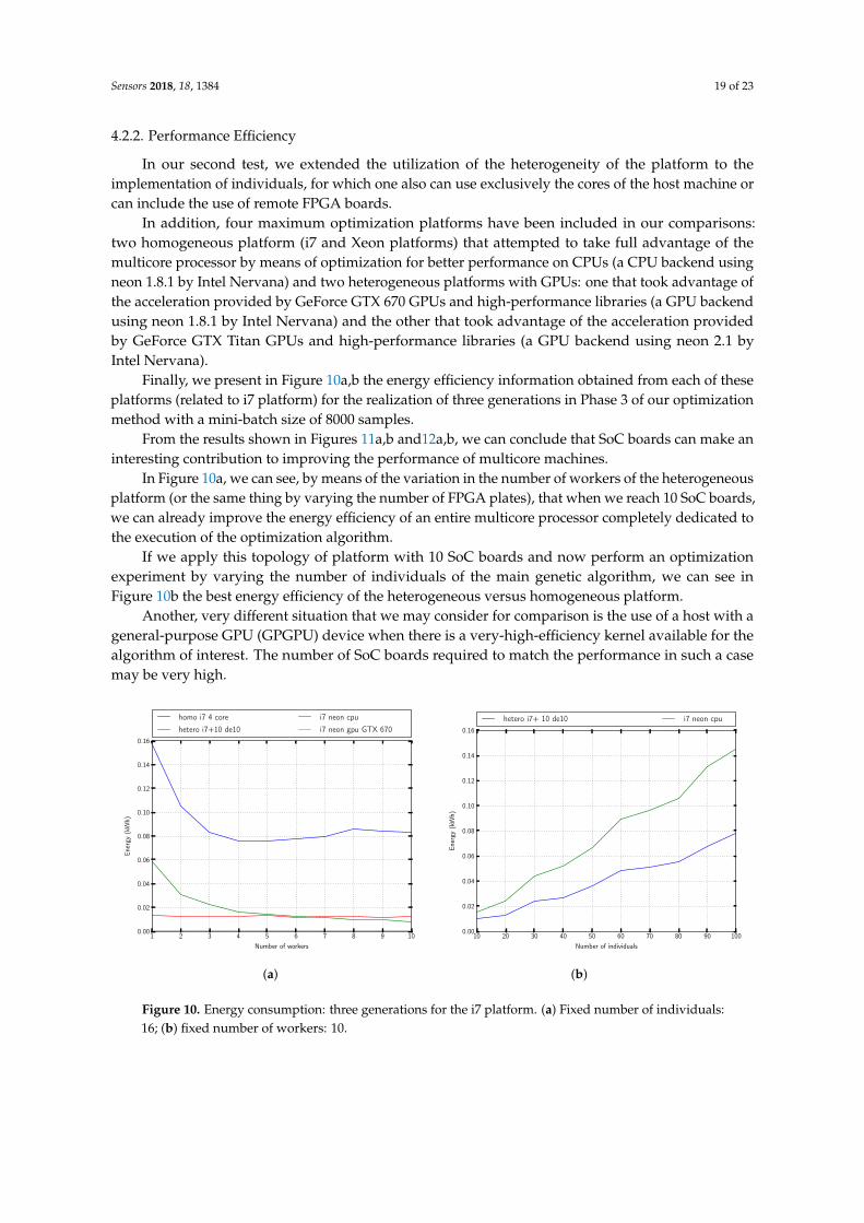
In addition, four maximum optimization platforms have been included in our comparisons:two homogeneous platform (i7 and Xeon platforms) that attempted to take full advantage of themulticore processor by means of optimization for better performance on CPUs (a CPU backend usingneon 1.8.1 by Intel Nervana) and two heterogeneous platforms with GPUs: one that took advantage ofthe acceleration provided by GeForce GTX 670 GPUs and high-performance libraries (a GPU backendusing neon 1.8.1 by Intel Nervana) and the other that took advantage of the acceleration providedby GeForce GTX Titan GPUs and high-performance libraries (a GPU backend using neon 2.1 byIntel Nervana).

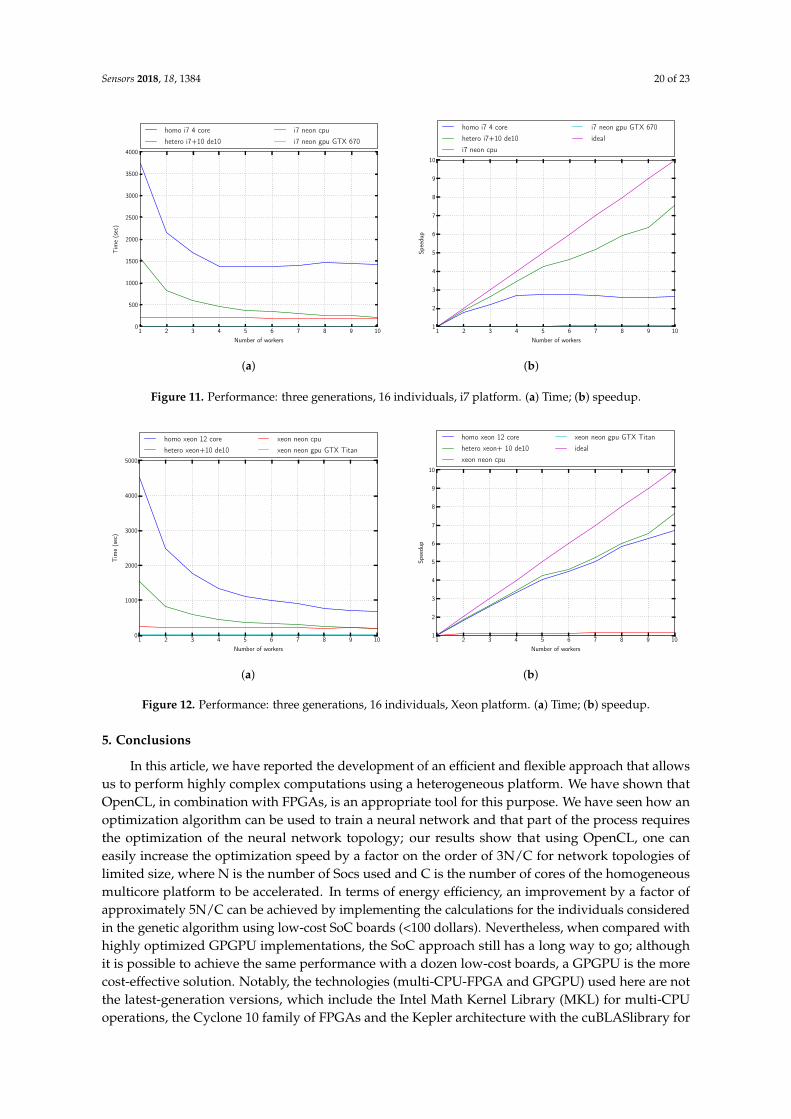
Finally, we present in Figure 10a,b the energy efficiency information obtained from each of theseplatforms (related to i7 platform) for the realization of three generations in Phase 3 of our optimizationmethod with a mini-batch size of 8000 samples.

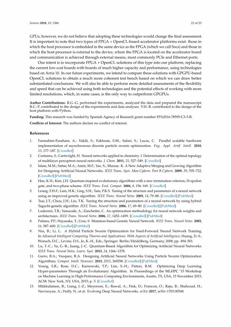
From the results shown in Figures 11a,b and12a,b, we can conclude that SoC boards can make aninteresting contribution to improving the performance of multicore machines.

In Figure 10a, we can see, by means of the variation in the number of workers of the heterogeneousplatform (or the same thing by varying the number of FPGA plates), that when we reach 10 SoC boards,we can already improve the energy efficiency of an entire multicore processor completely dedicated tothe execution of the optimization algorithm.

If we apply this topology of platform with 10 SoC boards and now perform an optimizationexperiment by varying the number of individuals of the main genetic algorithm, we can see inFigure 10b the best energy efficiency of the heterogeneous versus homogeneous platform.

Another, very different situation that we may consider for comparison is the use of a host with ageneral-purpose GPU (GPGPU) device when there is a very-high-efficiency kernel available for thealgorithm of interest. The number of SoC boards required to match the performance in such a casemay be very high.

Sensors 2018, 18, x 19 of 23

4.2.2. Performance Efficiency

In our second test, we extended the utilization of the heterogeneity of the platform to theimplementation of individuals, for which one also can use exclusively the cores of the host machine orcan include the use of remote FPGA boards.

In addition, four maximum optimization platforms have been included in our comparisons:two homogeneous platform (i7 and Xeon platforms) that attempted to take full advantage of themulticore processor by means of optimization for better performance on CPUs (a CPU backend usingneon 1.8.1 by Intel Nervana) and two heterogeneous platform with GPUs: one that took advantage ofthe acceleration provided by GeForce GTX 670 GPUs and high-performance libraries (a GPU backendusing neon 1.8.1 by Intel Nervana) and the other took advantage of the acceleration provided by GeforceGTX Titan GPUs and high-performance libraries (a GPU backend using neon 2.1 by Intel Nervana).

Finally, we present in Figure 10a,b the energy efficiency information obtained from each of theseplatforms (related to i7 platform) for the realization of 3 generations in phase 3 of our optimizationmethod with a minibatch size of 8000 samples.

From the results shown in Figures 11a,b and12a,b, we can conclude that SoC boards can make aninteresting contribution to improving the performance of multicore machines.

In Figure 10a we can see, by means of the variation in the number of workers of the heterogeneousplatform (or the same thing by varying the number of FPGA plates), that when we reach 10 Soc boards,we can already improve the energy efficiency of an entire multicore processor completely dedicated tothe execution of the optimization algorithm.

If we apply this topology of platform with 10 Soc boards and now perform an optimizationexperiment by varying the number of individuals of the main genetic algorithm, we can see inFigure 10b the best energy efficiency of the heterogeneous versus homogeneous platform.

Another, very different situation that we may consider for comparison is the use of a host with ageneral-purpose GPU (GPGPU) device when there is a very-high-efficiency kernel available for thealgorithm of interest. The number of SoC boards required to match the performance in such a casemay be very high.

1 2 3 4 5 6 7 8 9 10Number of workers

0.00

0.02

0.04

0.06

0.08

0.10

0.12

0.14

0.16

Ener

gy(k

Wh)

homo i7 4 corehetero i7+10 de10

i7 neon cpui7 neon gpu GTX 670

(a)

10 20 30 40 50 60 70 80 90 100Number of individuals

0.00

0.02

0.04

0.06

0.08

0.10

0.12

0.14

0.16

Ener

gy(k

Wh)

hetero i7+ 10 de10 i7 neon cpu

(b)

Figure 10. Energy consumption: 3 generations i7 platform. (a) Fixed number of individuals:16;(b) Fixed number of workers:10.Figure 10. Energy consumption: three generations for the i7 platform. (a) Fixed number of individuals:16; (b) fixed number of workers: 10.

Sensors 2018, 18, 1384 20 of 23Sensors 2018, 18, x 20 of 23


0

500

1000

1500

2000

2500

3000

3500

4000

Tim

e(s

ec)



(a)


1

2

3

4

5

6

7

8

9

10

Spee

dup

homo i7 4 corehetero i7+10 de10i7 neon cpu

i7 neon gpu GTX 670ideal

(b)

Figure 11. Performance: 3 generations, 16 individuals, i7 platform. (a) Time; (b) Speedup.


0

1000

2000

3000

4000

5000

Tim

e(s

ec)

homo xeon 12 corehetero xeon+10 de10

xeon neon cpuxeon neon gpu GTX Titan

(a)


1

2

3

4

5

6

7

8

9

10

Spee

dup

homo xeon 12 corehetero xeon+ 10 de10xeon neon cpu

xeon neon gpu GTX Titanideal

(b)

Figure 12. Performance: 3 generations, 16 individuals, Xeon platform. (a) Time; (b) Speedup.

5. Conclusions

In this article, we have reported the development of an efficient and flexible approach that allowsus to perform highly complex computations using a heterogeneous platform. We have shown thatOpenCL, in combination with FPGAs, is an appropriate tool for this purpose. We have seen how anoptimization algorithm can be used to train a neural network and that part of the process requiresthe optimization of the neural network topology; our results show that using OpenCL, one caneasily increase the optimization speed by a factor on the order of 3N/C for network topologies oflimited size, where N is the number of Socs used and C is the number of cores of the homogeneousmulticore platform to be accelerated. In terms of energy efficiency, an improvement by a factor ofapproximately 5N/C can be achieved by implementing the calculations for the individuals consideredin the genetic algorithm using low-cost Soc boards (<100 dollars). Nevertheless, when compared withhighly optimized GPGPU implementations, the Soc approach still has a long way to go; althoughit is possible to achieve the same performance with a dozen low-cost boards, a GPGPU is the morecost-effective solution. Notably, the technologies (multi-CPU-FPGA and GPGPU) used here are notthe latest-generation versions, which include the Intel Math Kernel Library (MKL) for multi-CPUoperations, the Cyclone 10 family of FPGAs and the Kepler architecture with the cuBLAS library for

Figure 11. Performance: three generations, 16 individuals, i7 platform. (a) Time; (b) speedup.

Sensors 2018, 18, x 20 of 23


0

500

1000

1500

2000

2500

3000

3500

4000

Tim

e(s

ec)



(a)


1

2

3

4

5

6

7

8

9

10

Spee

dup

homo i7 4 corehetero i7+10 de10i7 neon cpu

i7 neon gpu GTX 670ideal

(b)

Figure 11. Performance: 3 generations, 16 individuals, i7 platform. (a) Time; (b) Speedup.


0

1000

2000

3000

4000

5000

Tim

e(s

ec)

homo xeon 12 corehetero xeon+10 de10

xeon neon cpuxeon neon gpu GTX Titan

(a)


1

2

3

4

5

6

7

8

9

10

Spee

dup

homo xeon 12 corehetero xeon+ 10 de10xeon neon cpu

xeon neon gpu GTX Titanideal

(b)

Figure 12. Performance: 3 generations, 16 individuals, Xeon platform. (a) Time; (b) Speedup.

5. Conclusions

In this article, we have reported the development of an efficient and flexible approach that allowsus to perform highly complex computations using a heterogeneous platform. We have shown thatOpenCL, in combination with FPGAs, is an appropriate tool for this purpose. We have seen how anoptimization algorithm can be used to train a neural network and that part of the process requiresthe optimization of the neural network topology; our results show that using OpenCL, one caneasily increase the optimization speed by a factor on the order of 3N/C for network topologies oflimited size, where N is the number of Socs used and C is the number of cores of the homogeneousmulticore platform to be accelerated. In terms of energy efficiency, an improvement by a factor ofapproximately 5N/C can be achieved by implementing the calculations for the individuals consideredin the genetic algorithm using low-cost Soc boards (<100 dollars). Nevertheless, when compared withhighly optimized GPGPU implementations, the Soc approach still has a long way to go; althoughit is possible to achieve the same performance with a dozen low-cost boards, a GPGPU is the morecost-effective solution. Notably, the technologies (multi-CPU-FPGA and GPGPU) used here are notthe latest-generation versions, which include the Intel Math Kernel Library (MKL) for multi-CPUoperations, the Cyclone 10 family of FPGAs and the Kepler architecture with the cuBLAS library for

Figure 12. Performance: three generations, 16 individuals, Xeon platform. (a) Time; (b) speedup.

5. Conclusions

In this article, we have reported the development of an efficient and flexible approach that allowsus to perform highly complex computations using a heterogeneous platform. We have shown thatOpenCL, in combination with FPGAs, is an appropriate tool for this purpose. We have seen how anoptimization algorithm can be used to train a neural network and that part of the process requiresthe optimization of the neural network topology; our results show that using OpenCL, one caneasily increase the optimization speed by a factor on the order of 3N/C for network topologies oflimited size, where N is the number of Socs used and C is the number of cores of the homogeneousmulticore platform to be accelerated. In terms of energy efficiency, an improvement by a factor ofapproximately 5N/C can be achieved by implementing the calculations for the individuals consideredin the genetic algorithm using low-cost SoC boards (<100 dollars). Nevertheless, when compared withhighly optimized GPGPU implementations, the SoC approach still has a long way to go; althoughit is possible to achieve the same performance with a dozen low-cost boards, a GPGPU is the morecost-effective solution. Notably, the technologies (multi-CPU-FPGA and GPGPU) used here are notthe latest-generation versions, which include the Intel Math Kernel Library (MKL) for multi-CPUoperations, the Cyclone 10 family of FPGAs and the Kepler architecture with the cuBLASlibrary for

Sensors 2018, 18, 1384 21 of 23

GPUs; however, we do not believe that adopting these technologies would change the final assessment.It is important to note that two types of FPGA + OpenCL-based accelerator platforms exist: those inwhich the host processor is embedded in the same device as the FPGA (which we call Socs) and those inwhich the host processor is external to the device, where the FPGA is located on the accelerator boardand communication is achieved through external means, most commonly PCIe and Ethernet ports.

Our intent is to incorporate FPGA + OpenCL solutions of this type into our platform, replacingthe current low-cost boards with boards of much higher capacity and performance, using technologiesbased on Arria 10. In our future experiments, we intend to compare these solutions with GPGPU-basedOpenCL solutions to obtain a much more coherent test bench based on which we can draw bettersubstantiated conclusions. We will also be able to perform more detailed assessments of the flexibilityand speed that can be achieved using both technologies and the potential effects of working with morelimited resolutions, which, in some cases, is the only way to outperform GPGPUs.

Author Contributions: R.G.-G. performed the experiments, analyzed the data and prepared the manuscript.R.C.-P. contributed to the design of the experiments and data analyses. V.H.-B. contributed to the design of thehost platform with Python.

Funding: This research was funded by Spanish Agency of Research grant number FPA2016-78595-C3-3-R.

Conflicts of Interest: The authors declare no conflict of interest.

References

1. Farmahini-Farahani, A.; Vakili, S.; Fakhraie, S.M.; Safari, S.; Lucas, C. Parallel scalable hardwareimplementation of asynchronous discrete particle swarm optimization. Eng. Appl. Artif. Intell. 2010,23, 177–187. [CrossRef]

2. Curteanu, S.; Cartwright, H. Neural networks applied in chemistry. I. Determination of the optimal topologyof multilayer perceptron neural networks. J. Chem. 2011, 25, 527–549. [CrossRef]

3. Islam, M.M.; Sattar, M.A.; Amin, M.F.; Yao, X.; Murase. K. A New Adaptive Merging and Growing Algorithmfor Designing Artificial Neural Networks. IEEE Trans. Syst. Man Cybern. Part B Cybern. 2009, 39, 705–722.[CrossRef] [PubMed]

4. Han, K.H.; Kim, J.H. Quantum-inspired evolutionary algorithms with a new termination criterion, H-epsilongate, and two-phase scheme. IEEE Trans. Evol. Comput. 2004, 8, 156–169. [CrossRef]

5. Leung, F.H.F.; Lam, H.K.; Ling, S.H.; Tam, P.K.S. Tuning of the structure and parameters of a neural networkusing an improved genetic algorithm. IEEE Trans. Neural Netw. 2003, 14, 79–88. [CrossRef] [PubMed]

6. Tsai, J.T.; Chou, J.H.; Liu, T.K. Tuning the structure and parameters of a neural network by using hybridTaguchi-genetic algorithm. IEEE Trans. Neural Netw. 2006, 17, 69–80. [CrossRef] [PubMed]

7. Ludermir, T.B.; Yamazaki, A.; Zanchettin, C. An optimization methodology for neural network weights andarchitectures. IEEE Trans. Neural Netw. 2006, 17, 1452–1459. [CrossRef] [PubMed]

8. Palmes, P.P.; Hayasaka, T.; Usui, S. Mutation-based Genetic Neural Network. IEEE Trans. Neural Netw. 2005,16, 587–600. [CrossRef] [PubMed]

9. Niu, B.; Li, L. A Hybrid Particle Swarm Optimization for Feed-Forward Neural Network Training.In Advanced Intelligent Computing Theories and Applications: With Aspects of Artificial Intelligence; Huang, D.-S.,Wunsch, D.C., Levine, D.S., Jo, K.-H., Eds.; Springer: Berlin/Heidelberg, Germany, 2008; pp. 494–501.

10. Lu, T.-C.; Yu, G.-R.; Juang, J.-C. Quantum-Based Algorithm for Optimizing Artificial Neural Networks.IEEE Trans. Neural Netw. Learn. Syst. 2013, 24, 1266–1278.

11. Garro, B.A.; Vazquez, R.A. Designing Artificial Neural Networks Using Particle Swarm OptimizationAlgorithms. Comput. Intell. Neurosci. 2015, 2015, 369298. [CrossRef] [PubMed]

12. Young, S.R.; Rose, D.C.; Karnowski, T.P.; Lim, S.-H.; Patton, R.M. Optimizing Deep LearningHyper-parameters Through an Evolutionary Algorithm. In Proceedings of the MLHPC ’15 Workshopon Machine Learning in High-Performance Computing Environments, Austin, TX, USA, 15 November 2015;ACM: New York, NY, USA, 2015; p. 5. [CrossRef]

13. Miikkulainen, R.; Liang, J.-Z.; Meyerson, E.; Rawal, A.; Fink, D.; Francon, O.; Raju, B.; Shahrzad, H.;Navruzyan, A.; Duffy, N.; et al. Evolving Deep Neural Networks. arXiv 2017, arXiv:1703.00548.

http://dx.doi.org/10.1016/j.engappai.2009.12.001

http://dx.doi.org/10.1002/cem.1401

http://dx.doi.org/10.1109/TSMCB.2008.2008724

http://www.ncbi.nlm.nih.gov/pubmed/19203888

http://dx.doi.org/10.1109/TEVC.2004.823467

http://dx.doi.org/10.1109/TNN.2002.804317








http://dx.doi.org/10.1155/2015/369298


http://dx.doi.org/10.1145/2834892

Sensors 2018, 18, 1384 22 of 23

14. Real, E.; Moore, S.; Selle, A.; Saxena, S.; Suematsu, Y.L.; Le, Q.V.; Kurakin, A. Large-Scale Evolution of ImageClassifiers. arXiv 2017, arXiv:1703.01041.

15. Baker, B.; Gupta, O.; Naik, N.; Raskar, R. Designing Neural Network Architectures Using ReinforcementLearning. arXiv 2016, arXiv:1611.02167.

16. Yao, X. Evolving artificial neural networks. Proc. IEEE 1999, 87, 1423–1447.17. Yao, X.; Liu, Y. A new evolutionary system for evolving artificial neural networks. IEEE Trans. Neural Netw.

1997, 8, 694–713. [CrossRef] [PubMed]18. Mateo, F.; Sovilj, D.; Gadea-Gironés, R. Approximate k-NN delta test minimization method using genetic

algorithms: Application to time series. Neurocomputing 2010, 73, 2017–2029. [CrossRef]19. Hawkins, S.; He, H.; Williams, G.; Baxter, R. Outlier Detection Using Replicator Neural Networks.

In Proceedings of the Fifth International Conference on Data Warehousing and Knowledge Discovery(DaWaK02), Toulouse, France, 2 September 2002; pp. 170–180.

20. Fe, J.D.; Aliaga, R.J. Gadea-Gironés, R. Evolutionary Optimization of Neural Networks with HeterogeneousComputation: Study and Implementation. J. Supercomput. 2015, 71, 2944–2962. [CrossRef]

21. Prechelt, L. PROBEN1—A Set of Neural Network Benchmark Problems and Benchmarking Rules; Technical Report;The University of Karlsruhe: Karlsruhe, Germany, 1994.

22. Kingma, D.P.; Jimmy, B. Adam: A Method for Stochastic Optimization. arXiv 2014, arXiv:1412.6980.23. Zeiler, M.D. ADADELTA: An Adaptive Learning Rate Method. arXiv 2012, arXiv:1212.5701.24. MacKay, D.J.C. Bayesian Interpolation. Neural Comput. 1991, 4, 415–447. [CrossRef]25. Abbass, H.A. An Evolutionary Artificial Neural Networks Approach for Breast Cancer Diagnosis.

Artif. Intell. Med. 2002, 25, 265–281. [CrossRef]26. Ahmad, F.; Isa, N.A.M.; Hussain, Z.; Sulaiman, S.N. A genetic algorithm-based multi-objective optimization

of an artificial neural network classifier for breast cancer diagnosis. Neural Comput. Appl. 2013, 23, 1427–1435.[CrossRef]

27. Sarangi, P.P.; Sahu, A.; Panda, M. Article: A Hybrid Differential Evolution and Back-Propagation Algorithmfor Feedforward Neural Network Training. Int. J. Comput. Appl. 2013, 84, 1–9.

28. Bengio, Y.; Lamblin, P.; Popovici, D.; Larochelle, H. Greedy layer-wise training of deep networks. Adv. NeuralInf. Process. Syst. 2007, 19, 153.

29. Sankaradas, M.; Jakkula, V.; Cadambi, S.; Chakradhar, S.; Durdanovic, I.; Cosatto, E.; Graf, H.P. A MassivelyParallel Coprocessor for Convolutional Neural Networks. In Proceedings of the ASAP 2009 20th IEEEInternational Conference on Application-Specific Systems, Architectures and Processors, Boston, MA, USA,7–9 July 2009; pp. 53–60. [CrossRef]

30. Prado, R.N.A.; Melo, J.D.; Oliveira, J.A.N.; Neto, A.D.D. FPGA based implementation of a Fuzzy NeuralNetwork modular architecture for embedded systems. In Proceedings of the 2012 International JointConference on Neural Networks (IJCNN), Brisbane, Australia, 10–15 June 2012; pp. 1–7. [CrossRef]

31. Çavuslu, M.; Karakuzu, C.; Sahin, S.; Yakut, M. Neural network training based on FPGA with floating pointnumber format and it’s performance. Neural Comput. Appl. 2011, 20, 195–202. [CrossRef]

32. Wu, G.-D.; Zhu, Z.-W.; Lin, B.-W. Reconfigurable back propagation based neural network architecture.In Proceedings of the 2011 13th International Symposium on Integrated Circuits (ISIC), Singapore,12–14 December 2011; pp. 67 –70. [CrossRef]

33. Pinjare, S.L.; Arun Kumar, M. Implementation of Neural Network Back Propagation Training Algorithm onFPGA. Int. J. Comput. Appl. 2012, 52, 1–7.

34. Zhang, C.; Li, P.; Sun, G.; Guan, Y.; Xiao, B.; Cong, J. Optimizing FPGA-based Accelerator Design forDeep Convolutional Neural Networks. In Proceedings of the FPGA ’15 2015 ACM/SIGDA InternationalSymposium on Field-Programmable Gate Arrays, Monterey, CA, USA, 22–24 February 2015; ACM:New York, NY, USA, 2015; pp. 161–170. [CrossRef]

35. Wang, C.; Gong, L.; Yu, Q.; Li, X.; Xie, Y.; Zhou, X. DLAU: A Scalable Deep Learning Accelerator Unit onFPGA. IEEE Trans. Comput. Aided Des. Integr. Circuits Syst. 2017, 36, 513–517. [CrossRef]

36. Zhao, R.; Song, W.; Zhang, W.; Xing, T.; Lin, J.-H.; Srivastava, M.; Gupta, R.; Zhang, Z. Accelerating BinarizedConvolutional Neural Networks with Software-Programmable FPGAs. In Proceedings of the FPGA ’172017 ACM/SIGDA International Symposium on Field-Programmable Gate Arrays, Monterey, CA, USA,22–24 February 2017; ACM: New York, NY, USA, 2017; pp. 15–24. [CrossRef]

http://dx.doi.org/10.1109/72.572107


http://dx.doi.org/10.1016/j.neucom.2009.11.032

http://dx.doi.org/10.1007/s11227-015-1419-7

http://dx.doi.org/10.1162/neco.1992.4.3.415

http://dx.doi.org/10.1016/S0933-3657(02)00028-3

http://dx.doi.org/10.1007/s00521-012-1092-1

http://dx.doi.org/10.1109/ASAP.2009.25

http://dx.doi.org/10.1109/IJCNN.2012.6252447

http://dx.doi.org/10.1007/s00521-010-0423-3

http://dx.doi.org/10.1109/ISICir.2011.6131881

http://dx.doi.org/10.1145/2684746.2689060

http://dx.doi.org/10.1109/TCAD.2016.2587683

http://dx.doi.org/10.1145/3020078.3021741

Sensors 2018, 18, 1384 23 of 23

37. Bettoni, M.; Urgese, G.; Kobayashi, Y.; Macii, E.; Acquaviva, A. A Convolutional Neural Network FullyImplemented on FPGA for Embedded Platforms. In 2017 New Generation of CAS (NGCAS); IEEE: Piscataway,NJ, USA, 2017; pp. 49–52. [CrossRef]

38. Qiao, Y.; Shen, J.; Huang, D.; Yang, Q.; Wen, M.; Zhang, C. Optimizing OpenCL Implementation of DeepConvolutional Neural Network on FPGA. In Network and Parallel Computing; Shi, X., An, H., Wang, C.,Kandemir, M., Jin, H., Eds.; Springer International Publishing: Cham, Switzerland, 2017; pp. 100–111.

39. Suda, N.; Chandra, V.; Dasika, G.; Mohanty, A.; Ma, Y.; Vrudhula, S.; Seo, J.-S.; Cao, Y. Throughput-OptimizedOpenCL-based FPGA Accelerator for Large-Scale Convolutional Neural Networks. In Proceedingsof the FPGA ’16 2016 ACM/SIGDA International Symposium on Field-Programmable Gate Arrays,Monterey, CA, USA, 21–23 February 2016. [CrossRef]

40. Zhu, M.; Liu, L.; Wang, C.; Xie, Y. CNNLab: A Novel Parallel Framework for Neural Networks using GPUand FPGA-a Practical Study with Trade-off Analysis. arXiv 2016, arxiv:1606.06234.

41. Gadea-Giron, R.; Herrero, V.; Sebastia, A.; Salcedo, A.-M. The Role of the Embedded Memories in theImplementation of Artificial Neural Networks. In Proceedings of the FPL ’00 The Roadmap to ReconfigurableComputing, 10th International Workshop on Field-Programmable Logic and Applications, Villach, Austria,27–30 August 2000; Springer: London, UK, 2000; pp. 785–788.

c© 2018 by the authors. Licensee MDPI, Basel, Switzerland. This article is an open accessarticle distributed under the terms and conditions of the Creative Commons Attribution(CC BY) license (http://creativecommons.org/licenses/by/4.0/).

http://dx.doi.org/10.1109/NGCAS.2017.16

http://dx.doi.org/10.1145/2847263.2847276

http://creativecommons.org/

http://creativecommons.org/licenses/by/4.0/.

Documents

ID , Ricardo Colom-Palero and Vicente Herrero-Bosch