IP

AFIT/GAE/ENY/93D-29

AD-A273 984

A NUMERICAL DETERMINATION OF BIFURCATION

POINTS FOR LOW REYNOLDS NUMBER

CONICAL FLOWS DT 1CTHESIS

Larry K. Waters DEG 17 1993Captain, USAF

AFIT/GAE/ENY/93D-29

93-30639I 111 1li! 11111 III 11 11111Il11

Approved for public release; distribution unlimited

193 12 17037

"AFIT/GAE/ENY/93D-29

A NUMERICAL DETERMINATION OF BIFURCATION POINTS FOR LOW

REYNOLDS NUMBER CONICAL FLOWS

THESIS

Presented to the Faculty of the Graduate School of Engineering

of the Air Force Institute of Technology

Air University

In Partial Fulfillment of the

Requirements for the Degree of

Master of Science in Aeronautical Engineering

Accesion For

NTIS CRA&I

Larry K. Waters, B.S. DTIC TABUnannounced 0

Captain, USAF JL:stificationl .......................

ByDist ib,. ti.•, I

Av:aiiabfiity Codes

December, 1993 Av,:!i d / orDis C ial

Approved for public release; distribution unlimited

Acknowledgements

I would like to first thank my advisor, Dr. Beran, for his patience and understanding.

I would also like to thank the other members of my committee, Maj Buter and Dr. King,

for their support. Capt Morton deserves a special thank you. He was always willing to

make time in his busy schedule to give the advise and encouragement I needed to keep

going through some frustrating times. I would also like to thank my friends Doug Blake,

Paul Schubert, and Bernie Frank, who were always willing to sit and listen.

The people who deserve the most gratitude are my wife Charlotte and my son Mike.

As an ICU nurse, Charlotte has a job that is vastly more important than anything I do,

yet she always has time to listen patiently to my problems, and give me all the support

anyone could ever ask for. Mike had to endure endless excuses for why I had to spend

time with my school work instead of him. Any success I have had at AFIT is directly

attributable to Charlotte and Mike, my two best friends.

Larry K. Waters

Table of Contents

Page

Acknowledgements ........... .................................. ii

List of Figures ............. .................................... vii

List of Tables ........... ..................................... ix

Abstract ............ ........................................ x

I. Introduction ........... .................................. 1-1

1.1 Historical Background .............................. 1-2

1.1.1 Mach number effects ......................... 1-4

1.1.2 Geometric effects ............................ 1-4

1.2 Research Objective ................................ 1-6

11. Analysis ........ .................................... 2-1

2.1 Model Assumptions ........ ....................... 2-1

2.2 Linearization of Sutherland's Law ..................... 2-3

2.3 Governing Equations .............................. 2-6

2.4 73oundary Conditions ........ ...................... 2-8

2.5 Coordinate Transformation .......................... 2-9

2.6 Discretization of the Governing Equations and Boundary Con-

ditions ........................................ 2-13

2.7 Implementation of Continuity at the Freestream Boundary 2-14

2.8 Grid Generation and Discretization .................... 2-15

2.9 Added Numerical Dissipation ......................... 2-17

III. Solution Algorithm ......... .............................. 3-1

3.1 Newton's Method ......... ........................ 3-1

3.2 Continuation Method ..................... 3-2

iii

Page

IV. Navier-Stokes Solutions ......... ........................... 4-1

4.1 Supersonic Results ................................ 4-2

4.2 Subsonic Results ......... ......................... 4-4

V. Conclusions and Recommendations ............................ 5-1

Bibliography .......... ..................................... BIB-1

Appendix A. Derivation of Governing Equations ..................... A-1

Appendix B. Derivation of Analytical Jacobian Elements ............... B-i

Vita ........... .......................................... VITA-I

iv

"List of Symbols

Symbol Definition

F System of nonlinear equations

TF Jacobian matrix

I Number of nodes in the 0 direction

J Number of nodes in the 0 direction

M Freestream Mach number

P Pressure

Pr Prandtl number

R Gas constant

Re Reynolds number

T Temperature

U.o Freestream velocity

V Velocity vector

cl, c2 Coefficients from Sutherland's law

61, a2 Non-dimensional coefficients from linear p - e relationship

a,, Freestream speed of sound

dmin Initial wall spacing for packed grid

e Internal energy

f An arbitrary variable

u Velocity component in the radial direction

v Velocity component in the 0 direction

w Velocity component in the 0 direction

7 Solution to the system of nonlinear equations

K Coefficient of thermal conductivity

0, Cone half-angle

9.a: Angle at freestream boundary

a Angle of attack

aG, Angle of attack where symmetric vortices appear

v

Angle of attack where asymmetric vortices appear

QUV Angle of attack where unsteady vortices appear

A Coefficient of viscosity

p Density

^ Ratio of specific heats

A Second coefficient of viscosity

cV Specific heat at constant volume

CP Specific heat at constant pressure

vi

List of Figures

Figure Page

1.1. Mach number effects on a., (12) ........ ..................... 1-5

1.2. Possible Solution Spaces ......... .......................... 1-6

2.1. Comparison of Sutherland's law and linearized formula .............. 2-4

2.2. Spherical coordinate system and 2-D "plane" of constant r ....... .... 2-5

2.3. Physical and Computational Domains ....... .................. 2-10

2.4. Nine-point Stencil for interior nodes ........................... 2-13

2.5. Stencil for one-sided boundary derivatives ...... ................ 2-14

2.6. Stencil for Continuity equation at freestream boundary ............. 2-15

2.7. Node numbering in computational domain ...................... 2-17

2.8. Stencil for fourth-order dissipation ........ .................... 2-18

2.9. Uniform Grid .......... ................................ 2-19

2.10. Packed Grid .......... ................................. 2-20

3.1. Illustration of continuation procedure, Beran (4) .................. 3-5

4.1. Supersonic Flow over Cone at a = 0 ....... ................... 4-7

4.2. Non-dimensional density ......... .......................... 4-8

4.3. Non-dimensional u velocity component ....... .................. 4-9

4.4. Non-dimensional v velocity component ....... .................. 4-9

4.5. 30x81, Re = 500, M = .3,a = 5 deg ........................... 4-10

4.6. 30x81, Re = 500, M = .3,a = 8 deg ........................... 4-11

4.7. 30x81,Re=500,M= .3,a= 11 deg ....... ................... 4-12

4.8. 30x81, Re = 500, M = .3,a = 15 deg ....... ................... 4-13

4.9. 50x81, Re = 500, M = .3, a = 5 deg ........................... 4-14

4.10. 50x81, Re = 500, M = .3, a = 8 deg ........................... 4-15

vii

Figure Page

4.11. 50x81, Re = 500, M = .3,a = 11 deg ........................ 4-16

4.12. 50x81, Re = 500, M = .3, a = 15 deg ................... 4-17

4.13. 60x81, Re = 500, M = .3,a = 11 deg ................... 4-18

4.14. 60x81, Re = 500, M = .3, a = 15 deg ................... 4-19

B.1. Nine-point Stencil for interior nodes .................... B-2

viii

List of Tables

Table Page

2.1. Boundary conditions for supersonic flow ....... ................. 2-9

2.2. Boundary conditions for subsonic, inviscid flow ..... ............. 2-10

2.3. Boundary conditions for subsonic, viscous flow .................... 2-10

2.4. Node relationships for nine-point stencil ...... ................. 2-16

4.1. Initial boundary conditions for viscous subsonic flow ............... 4-2

4.2. Initial boundary conditions for inviscid subsonic flow ............... 4-2

4.3. Boundary conditions for subsonic, inviscid flow ...... ............. 4-7

4.4. Boundary conditions for subsonic, viscous flow .................... 4-7

4.5. Shock angle results ......... ............................. 4-8

4.6. Run Conditions for Point Solutions ........ .................... 4-8

ix

AFIT/GAE/ENY/93D-29

Abstract

It has long been established that supersonic flow over axisymmetric conical bodies

at high angles of attack tend to develop a side force due to vortical asymmetry. One

of the proposed reasons for the asymmetry is a bifurcation point in the solution of the

Navier-Stokes equations. This study investigated the possible existence of a bifurcation

point in the Navier-Stokes equations for subsonic laminar flow. Newton's method, with

gauss elimination, was used to solve the steady-state, viscous, compressible Navier-Stokes

equations in spherical cooordinates assuming conical similarity.

X

A NUMERICAL DETERMINATION OF BIFURCATION POINTS FOR LOW

REYNOLDS NUMBER CONICAL FLOWS

I. Introduction

Asymmetric vortices on the leeward side of slender conical bodies, such as missiles

or fighter aircraft flying at high angles of attack, can result in large side forces on the

body, even at zero yaw. These large side forces can have significance in vehicle directional

control. The development of symmetric and asymmetric vortices on the leeward side of

slender conical bodies has been observed for laminar and turbulent flows, subsonic through

hypersonic speeds, and various cross-sectional shapes (13).

Experimental studies of several researchers, including (29), (30), and (38), have identified

four distinct flow patterns about slender bodies at angle of attack and zero-degree sideslip.

Using 0, to denote the cone half-angle, a,, the angle of attack at which symmetric vortices

appear, a., the angle of attack at which asymmetric vortices appear, and a., the angle

of attack at which unsteady vortc shedding begins, the flow about a slender cone can be

characterized by:

1) At low angle of attack (0 < a < a,), axial flow dominates and the flow is attached.

2) At intermediate angles of attack (a,, < a < aa.), a symmetric vortex pair appears

on the leeward side of the body.

3) At higher angles of attack (a, _< •a < av), crossflow dominates and the vortices

become asymmetric. This results in rapidly increasing side forces, even at zero yaw.

4) At very high angles of attack (a,,, < a < 900), the crossflow dominates completely,

resulting in an unsteady vortex shedding similar to the Karman vortex shedding typical of

cylinders.

Ericsson and Reding (13), and Lowson and Ponton (23), report that for laminar flow,

a... 0 Oc, aa, ; 20c, and a,,, ; 600, whereas for turbulent flow a8,, z 1.30,.

1-1

1.1 Historical Background

In the late 1940's, lateral instability caused by asymmetric vortices was discovered

in flight tests. A great deal of experimental work followed, including Mudi et al. (25),

Peake et al. (29), Stahl et al. (30), Yanta and Wardlaw (38), and Zilliac et al. (39). One

of the original computational efforts was performed by Dyer et al. (11), who showed that

asymmetric vortices on the leeward side of a slender cone could be predicted by standard

line vortex models using symmetric boundary conditions. This study was followed up by

a more detailed study by Fiddes and Smith (15), and Fiddes (14), where vortex sheets

modeled by vortex filaments confirmed the earlier results. Assuming conical flow, Marconi

(24) used an algorithm based on the Euler equations to further demonstrate the existence

of the asymmetry in the vortex pair. In fact, Marconi found that at a critical angle of

attack, a•?, the symmetric solution was unsteady. He observed that the only way to achieve

a symmetric solution was to impose a symmetric condition.

In the late 1980's and early 1990's, more powerful computational tools brought a

virtual explosion to the area of calculating asymmetric vortical flow. Researchers such

as Marconi and Siclari (33), Siclari (32), Degani and Levy (9), Degani and Schiff (10),

Degani (7), Kandil et al. (19), Batina (3), and Vanden and Belk (36) are but a few of the

many computational efforts in this area. These studies range from subsonic to supersonic,

laminar and turbulent. Complementing the computational efforts were many experimental

studies, including Degani (8), Zilliac et al. (39), Modi et al. (25), Yanta and Wardlaw

(38), Lowson and Ponton (23), Peake et al. (29), and Stahl et al. (34). Many of these

efforts dealt with either the study of asymmetric vortices on different cross-sectional shapes,

including delta wings, or the suppression of the asymmetry using fins or strakes, which

impose a symmetry in the flow.

Several of the numerical solutions utilized the conical flow assumption: Batina (3),

Kandil et al. (19), Siclari (32), and Siclari and Marconi (33). With the conical flow as-

sumption, changes in the flow variables in the radial direction are neglected, so that the

governing equations may be solved in two dimensions. The advantage of using this assump-

tion is that a much more detailed numerical analysis can be performed. The disadvantage

is that only inviscid, supersonic flow is truly conical, where the length scale has disap-

1-2

peared from the problem. Ericsson (12) investigated experimental results for supersonic

and subsonic viscous flow and concluded that "conical flow asymmetry does indeed exist,

but only up to moderate angles of attack, a < 30 deg, where the axial flow component still

has a strong influence on the crossflow-separation characteristics."

All of the results from the studies that incorporated the conical flow assumption

show that asymmetric vortices develop around the critical angle a., z 20,. In the study

performed by Siclari and Marconi (33), when starting from a symmetric initial condition

the residual (difference between the exact and approximate solutions) declined by ten

orders of magnitude, and at this point the solution was essentially symmetric (Category

2 above). As the iterative scheme progressed, the residual increased to almost its original

value and then declined monotonically to machine zero where asymmetric vortices were

observed. Monotonic convergence to an asymmetric solution could be achieved, if a small

asymmetry was introduced into the initial condition. The same convergence behavior was

also seen in the study by Kandil et al. (19), who used a similar algorithm. These studies

utilized a time integration approach.

Other researchers, (7), (10), and (36), computed the unrestricted, three-dimensional

flow, over a slender ogive-cylinder body at angle of attack. Vanden and Belk (36) computed

both supersonic and subsonic flow. In both cases, a localized perturbation to the body

shape was needed for the asymmetric solution (Category 3) to be stable. They report that

this observation shows that vortex asymmetry at high angles of attack on slender bodies is

due to a convective instability resulting from an asymmetric upstream disturbance. Degani

(7) computed the subsonic laminar flow about a slender ogive-cylinder body. Solutions were

obtained for angles of attack ranging from a = 200 to a = 800 and a Reynolds number

(based on freestream conditions and cylinder diameter) of ReD = 200,000. Results at

a Mach number, M, of 0.2 and a = 200 showed the flow to be steady and symmetric.

The introduction of a space-invariant, time-invariant perturbation placed near the tip

only made a small change to the flow structure. At a = 400 the flow was steady and

symmetric, but became asymmetric with the introduction of the perturbation. The level

of the asymmetry depended on the size and location of the perturbation. When the

1-3

perturbation was removed, the flow returned to the symmetric case. These studies also

used a time integration approach.

There have been several speculations as to the discrepancy between the results ob-

tained with the conical flow assumption and those without the restriction. In regards to

the results obtained by Degani and Schiff (10), where asymmetric vortices only appeared

when a perturbation was introduced into the flow, Kandil et al. (19) report that the rea-

son for this is the result of "the smallest scale of the grid at the solid boundary and the

damping effect of the numerical dissipation in the axial direction, in addition to the grid-

fineness distribution." Vanden and Belk (36) claim that the approximate factorization in

the numerical scheme used by Siclari (32) introduced an error into the transient solution.

Complicating the comparitive analysis is the inability to achieve a perfectly symmet-

ric test in experimental work. If the asymmetry is caused by arbitrarily small perturbations

present near the nose tip of the model, then the asymmetry will be observed experimen-

tally, especially since machining processes used to construct the test models are not perfect,

and small surface imperfections will always exist. It is these imperfections, which can be

large compared to the model radius near the model tip, that could be responsible for flow

asymmetry.

1.1.1 Mach number effects. Several researchers, including (19), (12), (20), and

(13) have investigated the effect of Mach number on the angle of attack at which the

asymmetry appears and the relative strength of the vortices. Their conclusion is that as

Mach number increases, a., increases, while a,, is not affected. This trend can be seen in

Figure 1.1, from (12). Also, the relative strength of the side forces is greater at subsonic

speeds.

1.1.2 Geometric effects. Again, several researchers, (23), (38), (20), (32), and

(13), have studied the effect of different cross-sectional shapes, blunt versus sharp noses,

and different fineness ratios of bodies. The cumulative results indicate that as the body

becomes thinner (more elliptic), it becomes more resistant to the onset of the asymmetry.

1-4

aAV/8=4

3 -

2 -

0 5' >5.8S o5 >0.8

S7.5* >0.3S100 >0.3

0 2 3

M.

Figure 1.1 Mach number effects on a.,, (12)

1-5

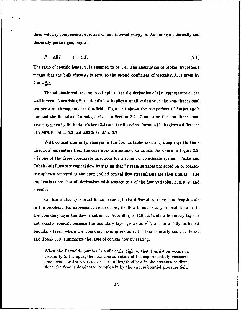
Figure 1.2 Possible Solution Spaces

Siclari found that asymmetric vortices develop for cross-sectional shapes other than circular

cones. His study included elliptic, biparabolic, and biwedge cross-sections.

Much lower side forces have been noted for blunt versus sharp nosed bodies. This

is possibly due to the fact that a bump near the nose, caused by surface roughness, has

greater impact on the sharp nose.

, Research Objective

The main objective of this study is to evaluate the solution space available to the

Navier-Stokes equations, assuming conical similarity, for flows around a slender, circular

cones at angle of attack. A direct numerical procedure is used to compute bifurcation

points in the solution space. At such points, symmetric vortex structures become unsta-

ble, while stable asymmetric vortex structures become admissable. Most of the previous

investigations in this area have dealt with the supersonic flow regime. This study provides

additional results for subsonic flow.

1-6

Figure 1.2 shows three possible solution spaces available for the Navier-Stokes equa-

tions. The first picture (a) represents the most likely solution space, and the one presented

by Siclari and Marconi (33). In these figures, the ordinate label is A, which represents a

free parameter in the solution. For this analysis, the free parameter is A = a/ec. The ab-

sicca represents a measureable quantity that changes after the bifurcation point is passed.

For this analysis, the side force coefficient is an applicable parameter. The trivial path is

designated as the path where the side force coefficient is zero. The point B represents the

the bifurcation point. To the left of B, the trivial path is the only solution available, and is

considered stable (s). To the right of B, the trivial path becomes an unstable solution (u),

and the pitchfork path represents the stable solution. There are two acceptable solution

paths, one above the ordinate and one below. These solutions are identical, mirror images

of each other. For this analysis, the two solutions represent which side of the cone the

asymmetry occurs on. The reason Newton's method with gauss elimination was chosen as

the solution technique for this study is because this combination, coupled with the continu-

ation method, allows for the systematic computation of the entire solution space, including

the unstable branches. Time integration techniques, used by other researchers, can not be

efficiently coupled with a continuation method. Also, considering the convergence behavior

experienced by Siclari and Marconi (33), time integration routines could result in different

solutions of the computed flowfield, depending on the convergence criteria used.

1-7

II. Analysis

In this Chapter, a model problem is formulated for the investigation of low-speed,

conical flows, including equations of motion, boundary conditions, and discretization. The

implications and validity of the assumptions of the model formulation are covered in Sec-

tion 2.1. Sutherland's law, used to model the coefficient of viscosity, is simplified through

linearization, described in Section 2.2. The non-dimensional governing equations, derived

in Appendix A, are presented in Section 2.3, while boundary conditions axe described in

Section 2.4. The coordinate transformation from physical to computational space is out-

lined in Section 2.5. Spatial discretization of the physical domain is covered in Section 2.6.

The approximation of the derivative terms in the governing equations and the boundary

conditions is shown in Section 2.7. The methodology for adding fourth-order numerical

dissipation is presented in Section 2.8.

2.1 Model Assumptions

The assumptions used in the analysis are:

"* Steady flow

"• Laminar flow

* Conical flow

* Thermally and calorically perfect gas

* Constant ratio of specific heats

* Linearized form of Sutherland's law

* Constant Prandtl number

"* Stokes' hypothesis

"* Adiabatic wall

* Normal pressure gradient at wall is zero

Steady flow implies _L = 0. In this context, and throughout the remainder of thisat

chapter, f represents any one of the five unknown variables in the problem: density, p, the

2-1

three velocity components, u, v, and w, and internal energy, e. Assuming a calorically and

thermally perfect gas, implies

P = pRT e = c,,T. (2.1)

The ratio of specific heats, -j, is assumed to be 1.4. The assumption of Stokes' hypothesis

means that the bulk viscosity is zero, so the second coefficient of viscosity, A, is given by

A = -

The adiabatic wall assumption implies that the derivative of the temperature at the

wall is zero. Linearizing Sutherland's law implies a small variation in the non-dimensional

temperature throughout the flowfield. Figure 2.1 shows the comparison of Sutherland's

law and the linearized formula, derived in Section 2.2. Comparing the non-dimensional

viscosity given by Sutherland's law (2.3) and the linearized formula (2.10) gives a difference

of 2.99% for M = 0.3 and 2.93% for M = 0.7.

With conical similarity, changes in the flow variables occuring along rays (in the r

direction) emanating from the cone apex are assumed to vanish. As shown in Figure 2.2,

r is one of the three coordinate directions for a spherical coordinate system. Peake and

Tobak (30) illustrate conical flow by stating that "stream surfaces projected on to concen-

tric spheres centered at the apex (called conical flow streamlines) are then similar." The

implications are that all derivatives with respect to r of the flow variables, p, u, v, w, and

e vanish.

Conical similarity is exact for supersonic, inviscid flow since there is no length scale

in the problem. For supersonic, viscous flow, the flow is not exactly conical, because in

the boundary layer the flow is subsonic. According to (30), a laminar boundary layer is

not exactly conical, because the boundary layer grows as r°5, and in a fully turbulent

boundary layer, where the boundary layer grows as r, the flow is nearly conical. Peake

and Tobak (30) summarize the issue of conical flow by stating:

When the Reynolds number is sufficiently high so that transistion occurs inproximity to the apex, the near-conical nature of the experimentally measuredflow demonstrates a virtual absence of length effects in the streamwise direc-tion: the flow is dominated completely by the circumferential pressure field.

2-2

Thus, the characteristics of these flow fields can be determined through mea-surement or by computation at essentially one streamwise station. In fullyturbulent and fully laminar subsonic freestream flow, even though base andthickness effects become measureable, the circumferential pressure gradientsstill dominate, to the extent that virtual conicity of the separation lines andshear-stress directions are still maintained.

The applicability of the conical flow assumption for subsonic flows is the subject of a

paper by Ericsson (12). In this paper Ericsson reviewed experimental results and concluded

that "conical flow asymmetry does exist on very slender cones because of the still-present

strong axial flow component at 20c < a < 30°." On cones where the asymmetry does not

develop until a > 30*, the flow is nonconical. For this reason, the cone half-angle used in

this study is 0, = 5 degrees.

The assumptions of a thermally and calorically perfect gas, along with constant

ratio of specific heats, is valid for the subsonic and low supersonic flows investigated in

this study (2). Reference (37) supports the assumption of constant Pr and zero pressure

gradient normal to the wall in the boundary layer. Symmetric and asymmetric vortices

have been shown to exist in flows over circular cones for steady, laminar flow (References

(13), (19), (33), (7)). No attempt was made to model turbulent flows.

2.2 Linearization of Sutherland's Law

Since viscosity is not assumed to be a constant, a relationship is desired that expresses

viscosity in terms of one or more of the unknown variables. Sutherland's law (1) provides

this relationship:

1u(T) = cf+T ' (2.2)

C2 + TV

where c2 = 110.4*K and cl will be eliminated through non-dimensionalization. Using

(2.1), M• can be expressed as a function of the internal energy, e. However, with this

expression, the complexity of the derivation of analytical Jacobian elements is greatly

increased. (examples of the derivation of Jacobian elements appear in Appendix B). To

avoid such complexity, (2.2) is first placed in non-dimensional form and then linearized to

provide a simpler expression for t.

2-3

2.00

1.50

S1. 0 00U

0.500.50Sutherland's formula

Linearized formula

0.00 ...... .......0.00 0.50 1.00 1.50 2.00 2.50

Temperature

Figure 2.1 Comparison of Sutherland's law and linearized formula

The freestream viscosity is found by evaluating (2.2) at the freestream temperature,

Too. The appropriate non-dimensional scale factors for p and T are then the freestream

values, t,,. and Too (all of the non-dimensional scale factors are given in Appendix A).

Using the superscript (*) to denote a non-dimensional value, equation (2.2) is written in

non-dimensional form as

= p(T) cT'12 (c2 +T.) (T' 3 12 c2/Too + 1A (T.) (c•2 + T) c1Tgi 2

T .PT') c2/To + T/T. (2.3)

Using T" = T/Too and c2 = c2/Too, (2.3) is rewritten as

A*(T*) = (To)3 1 2 C + 1 (2.4)(c,. + To)"

Equation (2.4) is linearized by expanding it in a first-order Taylor series expansion aboutTý•:

A= pA(T) + AT- + O(AT) 2 . (2.5)

2-4

Srr

U..

Figure 2.2 Spherical coordinate system and 2-D "plane" of constant r

Differentiating equation (2.4) with respect to T° gives

aT - (c +T)2 [(T*) 12(c; + T*) - (T*)312 (2.6)

2 ( + T'.)2

OP-J 2- (c2+1)" (:'.7)

Substituting (2.7) into (2.5), along with AT* = T° - T;, T* - 1, gives

3= [_ + ] (T -1) +1. (2.8)

Now, T" is replaced with e', one of the unknown non-dimensional variables, using

e = c ,,T = - )

2_5

where e and T are non-dimensionalized using the scale factors provided in Appendix A,

resulting in

U2 e = RTT- )" = T* = y(7 - 1)M2e*. (2.9)

Substituting (2.9) into (2.8) results in a linear, non-dimensional form of U in terms of the

internal energy:

U* = 61e* + c2, (2.10)

where Z1 and e 2 are given by:

e = [ _ -1 ] Y(-_1)M2, 2=1- (2.11)

The thermal conductivity, r, is related to jA through the assumption of a constant Prandtl

number, Pr, where

Pr - %# (2.12)K

Non-dimensionalization of (2.12) yields

Pr-= %KA*Aoo Pr = A*Pr. (2.13)

When Pr = constant, (2.13) provides

= K*. (2.14)

Equation (2.10) is used to replace the non-dimensional thermal conductivity, K*, which

appears in the energy equation (derived in Appendix A) For the remainder of the analysis,

the superscript (*), representing a non-dimensional variable, is dropped for convenience.

2.3 Governing Equations

Following the assumptions outlined in Sections 2.1 and 2.2, the non-dimensional

governing equations are developed in Appendix A. A schematic of the spherical coordinate

system is given in Figure 2.2. With the subscripts 0 and 4 denoting differentiation, the

2-6

non-dimensional governing equations in spherical coordinates are:

Continuity equation

2pu sine + pv cos0 + vpo sine + pvo sine + pwO + wpo = 0 (2.15)

r-momentum equation

pr sine I Ree We sine sin-2 0

+le + ý2 [8u 7v coto 7ve 7wo u__ 1o+ Re 3 3 3 3sin si 2 0 -U8 Cot j0 (2.16)R---3- + _3 + -3- +! 3sin0 s sin 00

8-momentum equation

pr vv0+ s + UV- W2cot +r(7-1) Le,+ep,]

4e9e 2v cot6 2wo 4vo 2u 1 jee nvcoso We vO+ ke 3 3 sine 3 3+ Re I sin20 sine sin 2

0o

+ _e + 62 2 7wo cosO 2 4vas v9Re 12v+ 3sin 20 + 2vcot80 sin 20

WOO 8uo 4vg coto 2v2 (2.17)3sine 3 3 3•sin 0(

0-momentum equation

pr vwowo o+ wu + VWcot + r(7--1) [ ep

sin [ + pe9]

w1e F v~ot 1+ 1e 4wo + 2u +4v cosG 2v. 1Rie n-sien Re 3 sin 20 3 sine 3Tsin 2T 3 sineJ

61 e + 62 [ 4w +o v+o + 8u + 7vo cosORe [3 sin20 + 3 sine 3 sine + -sin 2-

- 2w + sin2- +wocotG-2wcot 2 ] =0 (2.18)

Energy equation

pr ves + s-i~nO] + (y - 1)rep u + vcoto + Vo + yp e+sine sine

2-7

-y(ýIe + c2) ea Coto + eop + 1~ Yle2+ 06

PrRe ISin 29 PrRe 0sin 2 0

ele + e 2 f4v,2 4uve 4 U2 +4WO 4 V2 Cot 2 1Re 3 3 3 sin2G + 3

+4u,+ 8vw, cot 4uv coto v2+ 4sn+ 3 sine + + 2 + w + W 2 cot 20

2 wevo 2wv, coto 2 o + u2 2wu,+ O sCo + 0 sin20 sine

W,2 +V2 +U2 4vow, 4vv# oto(+w +u - 2vu- 3sinO 3 0 (2.19)

2.4 Boundary Conditions

The governing equations are solved at all the internal nodes, therefore only two

physical surfaces require boundary conditions. These surfaces are shown in Figure 2.2,

where the inner circle represents the wall boundary, and the outer circle represents the

freestream boundary. For the wall, the pressure derivative normal to the wall is set equal

to zero, and an adiabatic wall condition is used for all the runs. This implies,

aPOn 0 (2.20)

OT-5-n = 0 (2.21)

These boundary conditions are used in all the other computational efforts in this area (7),

(10), (19), (32), (33), and (36). The normal pressure derivative can be considered a first

step approximation, where a more accurate boundary condition would be setting normal

momentum equal to zero. Using equation (A.12), which relates pressure to density and

internal energy using the perfect gas assumptions, along with equation (2.9), which relates

temperature to internal energy, equations (2.20 - 2.21) can be expressed as

Op_O'n = 0 (2.22)

O9e_On = 0 (2.23)

2-8

Wall Freestream Boundary°-e=Op=l

SOnR 0 U -- Ups

V=0 V--Vf,

W=0 W=0Baeo

Table 2.1 Boundary conditions for supersonic flow

For the viscous flow cases, no slip at the wall is enforced: u = v = w = 0. For the inviscid

flow cases, slip flow and impermeability give 2u = 0, =0, and v =0.

On the freestream boundary (denoted by the subscript fs), a general set of equations

is used to determine the values for the flow velocities in terms of the angle of attack, a,

and the coordinate angles, 0 and q¶:

U1 = cosacos0 u2 = sinasin0coso u, = (u 2 + u•)'f 2 (2.24)

v' = - cosasin0 v2 = sinacos0cos 0 vf = (Viv• 2 (2.25)

W1 = 0 t = -sinasin wp = (w• +w- (2.26)

Equations (2.24 - 2.26) are also used to initialize the flow velocities.

An expression for non-dimensional internal energy at the freestream boundary, e,,

is obtained by evaluating equation (2.9) at T;, = 1. Therefore (dropping the (*) for

convenience),

e1 o = _(- 1)M2' (2.27)

The boundary conditions for each case are summarized in Tables (2.1 - 2.3). For sub-

sonic flow, the continuity equation is used as a freestream boundary condition. Section 2.6

outlines the use of the continuity as a boundary condition.

2.5 Coordinate Transformation

In computational fluid dynamics, the governing equations and boundary conditions

are solved at a finite number of discrete points which represent the solution domain. In

2-9

Wall Freestream Boundary-0 continuityIn Ul V2 W2=1

V 0 + =v=O p=l

O" =0 W "- Wf,

= 0 e = ef,

Table 2.2 Boundary conditions for subsonic, inviscid flow

Wall Freestream Boundary'a =continuityu=0 U2 + V2 +w 2 =l

v=0 p=1W 0 W =Wf,

ke = 0 e = efs

Table 2.3 Boundary conditions for subsonic, viscous flow

I~i

Figure 2.3 Physical and Computational Domains

2-10

the physical (0, 8) space, grid points need to be clustered near the wall so the boundary

layer can be properly resolved. This can be achieved by either uneven spacing between

grid points in the radial direction, or by placing many mor2 evenly spaced points along

each radial line. Clearly the first approach is more efficient computationally. However,

the standard second-order-accurate difference approximations used in the discretization

of the governing equations require a uniform spacing between nodes. Even spacing is

obtained, with node clustering in the physical domain, through a coordinate transformation

of the physical domain to a computational domain. In this problem, the physical space

is designated by the coordinate pair (0, 8), and the computational space is designated by

the coordinate pair (ý, 17), where Figure 2.3 shows the mapping between the two domains.

For this study, the physical domain could be separated anywhere, but the windward side

of the cone was selected because the gradients in the dependent variables are smaller in

this region. Using subscripts to denote differentiation, the transformation, from (16), is

expressed in general terms as

0 = 0(ý, 7), 0 = (V, 77), (2.28)

which, from the chain rule of partial differentiation, leads to

do = Ocdý + 0,7,d7, dO = Ofdý + 0j,. (2.29)

Similarly, the reverse transformation yields

ý -- ,($, 09), 77 = 77(0, 0), (2.30)

dý = ý.ddO + ýOdO, d77 = 77odk + qiodO. (2.31)

When expressed in matrix form, the transformation is

O f On 1 174[z ]J[ FL I71 77o OC =J -OC Ot

where the Jacobian is defined as

J = Oc,, - 0,70C.

2-11

The metrics of the transformation are

O9 9• O _•'=•- °=- •- 7 70- -

The metrics and the Jacobian are evaluated numerically at all node points in the domain

using the difference approximations provided in Section 2.7.

The spatial derivatives are transformed from physical to computational space with

the following formulas, from (16) and (35),

fo = fc + "n-•ff, fe = GAf( + 'ief", (2.32)

f#0= 2ff + 2tO,71ff + 72fqI7

- (•0• + 2ýi7OOf + %,7o1)(ýeff + ,jefj)

- (•bk + 20 + ) + 710f7), (2.33)

fe 02ff + ýjef + i~2f,

- ,90f + 2tie~, + i7q2i,),))(ýefC + iief,,)

- �•� 2 ý9oi90on + 2o702qn)(ýOf + 7o/fn), (2.34)

=e Wof + (7#ý + f*7)f, + 7777A

+ (iOeo + Woon - WoJt - 719GJq) A

- (eo0t + IbOt + 77o7joJn + 64Jt), (2.35)

-4 -= G, + Io0e + •4t + o0t, (2.36)

J- = Wtn + 77o0,7n + 740,777 + GOO" (2.37)J

2-12

knw kn kne

kw k ke

ksw ks kse

Figure 2.4 Nine-point Stencil for interior nodes

2.6 Discretization of the Governing Equations and Boundary Condi4 is

Following the transformation of the governing equations to the (ý, YI) computational

space, the spatial derivatives are approximated to second-order-accuracy with discrete

central-difference formulas. First and second derivatives of ý and q/, as well as cross-

derivative terms, appear in the transformed equations. Application of central-difference

formulas at a given node, k, requires information from adjacent node points. For the

central-difference formulas required in this study, the influential neighbors of an interior

node point are contained within a nine-point computational stencil, shown in Figure 2.4.

The difference approximations, from (1), used for the interior nodes, are

fkI - fi. (2.38)

f7Ik = ,- A (2.39)

Iflk "- , - 2 fk + . (2.40)

fnk = An - 2fk + Ik, (2.41)A77

,Ik= 1 (fke -[e 2n )" (2.42)

2-13

knn

kn

"Sw . k 1- ke

Figure 2.5 Stencil for one-sided boundary derivatives

For the wall boundary nodes, normal derivatives are replaced directly with rl deriva-

tive terms. One-sided, second-order-accurate difference approximations are used to ap-

proximate the Yj derivatives:

-34 + 4fkn - fn(S= ' (2.43)

where Figure 2.5 shows the stencil used for the one-sided differences needed for the bound-

ary derivatives. A square node arrangement is used for all cases, so Af = A77= 1.

2.7 Implementation of Continuity at the Freestream Boundary

For subsonic flow, the continuity equation (2.15) is used as a freestream boundary

condition. This equation is written as

2pu sinO + (pv sinO)e + (pw), = 0 (2.44)

The equation is rewritten in this form so that the first and second terms can be

evaluated at the midpoint between the boundary node and the next node in from the

boundary, shown in Figure 2.6. The difference approximation (2.36) is used to represent

the f derivative term. The first term is represented by averaging the values at the midpoint.

2-14

kw k ke-

Iks

-

Figure 2.6 Stencil for Continuity equation at freestream boundary

A second-order-accurate difference about the midpoint is used to represent the q derivative

term, so only two node points are required. The approximation equation is

A -fA. (2.45)

All of the grids used in the study have evenly spaced radial lines around the cone, covered

more extensively in section 2.7. This results in the metrics, te and 1, being zero. Therefore

the continuity equation used for the freestream boundary equation is

(pu sinO)k + (pu sinO)k, + '/e [(pv sinO)k - (pv sinO)h,]

+ -- [(pw)ke - (PW)k.] = 0. (2.46)

2.8 Grid Generation and Discretization

Two different grids are used in the analysis. The first is used for the inviscid cases,

both supersonic and subsonic. For these cases, there is no boundary layer to resolve so

there is no need to cluster the points near the cone surface. Therefore, the radial lines

are evenly spaced around the cone, and the points are evenly spaced along each radial

line. When the flow is viscous and subsonic, node points must be clustered near the cone

surface to accurately resolve the boundary layer. The radial lines are still spaced evenly

around the cone, but the nodes along each radial line are distributed using a geometric

progression, outlined in (6). Figures (2.9) and (2.10) show examples of the different grids.

The nodes in the computational domain are numbered using a row-by-row convention,

as shown in Figure 2.7. The advantage of numbering the nodes this way, as compared to

2-15

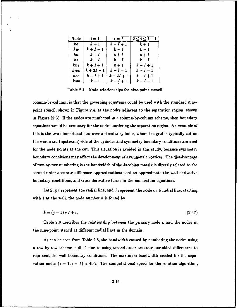
Node i= 1 i = I 2 < i < I- 1ke k+1 k-I+1 k+1kw, k+l-1 k-i k-1kn k+I k+I k+Iks k-I k-I k-I

kne k+I+1 k+i k+I+1knw k+21- 1 k + I-1 k + I-1kse k- I + 1 k-21+1 k- I + iksw k-1 k-I+i k-I-1

Table 2.4 Node relationships for nine-point stencil

column-by-column, is that the governing equations could be used with the standard nine-

point stencil, shown in Figure 2.4, at the nodes adjacent to the separation region, shown

in Figure (2.3). If the nodes are numbered in a column-by-column scheme, then boundary

equations would be necessary for the nodes bordering the separation region. An example of

this is the two-dimensional flow over a circular cylinder, where the grid is typically cut on

the windward (upstream) side of the cylinder and symmetry boundary conditions are used

for the node points at the cut. This situation is avoided in this study, because symmetry

boundary conditions may affect the development of asymmetric vortices. The disadvantage

of row-by-row numbering is the bandwidth of the Jacobian matrix is directly related to the

second-order-accurate difference approximations used to approximate the wall derivative

boundary conditions, and cross-derivative terms in the momentum equations.

Letting i represent the radial line, and j represent the node on a radial line, starting

with 1 at the wall, the node number k is found by

k= (j- 1)*I+i. (2.47)

Table 2.8 describes the relationship between the primary node k and the nodes in

the nine-point stencil at different radial lines in the domain.

As can be seen from Table 2.8, the bandwidth caused by numbering the nodes using

a row-by-row scheme is 41+1 due to using second-order accurate one-sided differences to

represent the wall boundary conditions. The maximum bandwidth needed for the sepa-

ration nodes (i = 1, i = I) is 41-1. The computational speed for the solution algorithm,

2-16

k=J1)1+l11 r•I

k=21+1 , 0 31

k=I+l - -21

k=1 2 3 4 ... I-i I

Figure 2.7 Node numbering in computational domain

outlined in Chapter III, is largely determined by the bandwidth of the Jacobian matrix.

As the bandwidth is increased, the time required for convergence increases exponentially.

2.9 Added Numerical Dissipation

For the subsonic, viscous flow cases, fourth-order numerical dissipation is added to

provide numerical smoothing. This smoothing diminishes the very small oscillations in

the computed flow variables present in the solutions near the freestream boundary, caused

by a lack of grid resolution. The added dissipation also affects the numerical results

near the body, so care must be taken when determining the amount of extra dissipation

added. Figure 2.8 shows the stencil needed for the added dissipation. The difference

approximations, from (1), for fourth-order spatial derivatives are

84f = w. (fkee 4fte + 6fk 4w+fk• w 7) (2.48)-8

84 770 We-74 - (fk- 4fk. + 6fk - 4fk + fko) (2.49)

077 8

where we is an adjustable parameter.

2-17

knn

kn

kww kw k ke kee

ks

kss

Figure 2.8 Stencil for fourth-order dissipation

2-18

10 Uniform Spacing 40X81

5

0

-5

-10-10 -5 0 5 10

Figure 2.9 Uniform Grid

2-19

60x81 Packed Grid7.5

5.0

25

0.0

-2.5

-5.0

-7. -

-5 0 5 10

FiEgre 2.10 Packed Grid

2-20

III. Solution Algorithm

3.1 Newton's Method

Newton's method is an iterative scheme that solves the nonlinear system of equations of

the form

S= 0, (3.1)

where X is a vector of N unknowns, and F is a set of N equations. The Newton iteration

formula is

-(VI+I _V) = _7(v), (3.2)

where T.- is the Jacobian matrix, whose elements are given by

OF. OF& ... OF.0:1 0:2 oz.

OFa OF . OF2

T7= 1 OI O2 ax. (3.3)

aF aF ... afF-OF.. OF. OF..ax0, 8:3 ax.~

V" represents a known solution state that is improved with the solution of (3.2), AT =

7'+' - V". Using central differences and a nine-point stencil to represent the derivatives

in the governing equations, (3.2) results in a banded system that is solved using Gauss

elimination. The solution of the system is AY = Y'+' - 7". After each iteration, the

approximate solution is updated by 7'+' = AY + 7". Successive iterations are computed

until the largest absolute A- is less than some small value c, or reaches machine zero.

Newton's method is guaranteed to converge quadratically if the Jacobian matrix is non-

singular and the initial guess is sufficiently close to the exact solution (18).

The analytical Jacobian elements are determined by differentiating each of the equa-

tions with respect to the unknown variables. An example of how these elements are derived

is shown in Appendix B. For the discrete equations in this study, the Jacobian elements are

3-1

relatively complicated. There is always the chance that there are errors in the derivation

and implementation of the elements. There are two methods of checking the accuracy of

these elements. The first is if the scheme is quadratically convergent, then the Jacobian

matrix is considered to be correct. The second method is to compare the analytical Ja-

cobian elements with elements developed numerically. Using a method implemented by

Morton (27), the elements of the two matrices are compared numerically, and when they

are equal the analytical elements are considered correct. This numerical scheme consists

of solving the function evaluation (right-hand side) for a given solution vector, i, at each

node, and then perturbing the solution vector by a small amount, Y + c, and then solving

the function evaluation with the perturbed solution vector. Subtracting the two results

for each unknown at each node in the nine-point stencil results in the numerical Jacobian

elements. Since a finite perturbation is used (c = 0.000001), the accuracy of the numerical

elements is taken to be oae order less than the c used. Use of this method allows for a

systematic way of checking each of the Jacobian elements, since any differences in the two

Jacobian matrices leads directly to the probable incorrect element. This allows the analyt-

ical Jacobian matrix to be verified with confidence in a short period of time. Without this

type of comparison, there is always the possibility that incorrect development or imple-

mentation of the analytical Jacobian elements is the cause of any difficulties in obtaining

a correct solution.

3.2 Continuation Method

It has been proven that if a solution Y* is known and T- is nonsingular, then for

some range of A about \* there exists a unique solution path through (Y*, A•). The proof

is outlined in (21). Pseudo-arclength continuation (PAC) is Keller's method of computing

solutions along the solution path by using information at (Y*, A*). to compute the next

solution point.

Figure 3.1 is representative of a solution path found by plotting the norm of the

solution vector versus the free parameter A. The PAC process is to compute a tangent

vector T at a known solution V, designated by P. Then at a distance d away, search along

a line perpendicular to T for the next solution point. This is done by first using arclength

3-2

to parameterize the solution path (X = Y(s),A = A(s), and F = T(s) = 0). Then the

tangent vector is computed by

d -(Y(s); A(s)) = 0. (3.4)

Using the chain rule, equation 3.5 becomes

TF1(s)y(S) + T-\(S),(S) = 0, (3.5)

where

(S) = •-•(S), (3.6)

and

= dA (3.7)

The definition of arclength is

I11112 + =2(S) = 1. (3.8)

Equations 3.5 and 3.8 can then be solved as a system for the tangent vector:

T(s) = (i(s)), (3.9)

providing the Jacobian matrix is not singular. Now define 4 such that

¢ = FrjF(s). (3.10)

Then equations 3.5 and 3.8 give the following relationships

-- = 1 (3.11)

and

X(s) = -A(s)q. (3.12)

The sign of equation 3.11 represents the direction of the tangent vector and is therefore

indeterminate. At the startup of the continuation process this sign is set depending on

which part of the solution path is to be computed.

3-3

From the solution P, the tangent vector T, and the distance d, the initial solution

vector Qo can be computed:

T (( ) +d ). (3.13)

solution Q lies on a line perpendicular to T passing through Qo. This condition can

be stated mathematically as

D =- i(YQ - Yp) + (AQ - Ap)Ap = d (3.14)

and can be added to the system of nonlinear equations 3.1. This new system is then solved

by Newton's method with Q0 as the initial guess. Q0 becomes a better and better first

approximation as d gets smaller. The solution XQ is obtained when F = 0 and D = d.

Another F 'ion can be computed by repeating the process.

The entire section on the continuation method was taken directly from Morton (26).

3-4

QQ

P Qd

Figure 3.1 Mustration of continuation procedure, Beran (4)

3-5

IV. Navier-Stokes Solutions

Initially, the boundary conditions in Table 4.1 were used to solve the subsonic flow

over a slender cone at zero angle of attack. These boundary conditions are the same as

those used by Degani and Schiff (10) in their three-dimensional analysis. However, when

these boundary conditions are used, oscillations (odd-even decoupling) developed in the

computed flow variables p, u, v, w, and e. A significant amount of effort was spent trying

to find an error in the code that would account for an error of this type. The derivation of

the governing equ .ions was checked by two independent methods, outlined in Appendix

A. The derivation of the analytical Jacobian elements and their implementation in the

code was checked using the numerical procedure outlined in Chapter III. The placement

of the Jacobian elements into the matrix was checked extensively, especially in the grid

separation region. Finally, a comparison was made with a 1-D inviscid code at a = 0, using

the boundary conditions in Table 4.2. These boundary conditions represent slip flow and

impermeability at the wall boundary. The two methods gave the same numerical result,

both having oscillations in the computed solution. The addition of fourth-order numerical

dissipation, outlined in Chapter 2.9, did not reduce the oscillations. Next, the boundary

conditions in Table 4.2 were used for a supersonic inviscid model at a = 0, and the solution

matched that of exact methods, both in shock angle and velocity components. The results

of this analysis is presented in Section 4.1. This analysis helped to verify the correctness

of some of the computer code, especially the implementation of the Jacobian elements in

the separation region. At this stage, the freestream boundary conditions were suspected

as the cause of the oscillatory behavior in the solution.

Several attempts were made to develop freestream boundary conditions for which

the solution would be free of oscillations. Several variations were attempted, and the

boundary conditions outlined in Table 4.3 and Table 4.4 were found to give good results.

The key to the problem is how the continuity equation is implemented at the discrete node

points. Initially, the continuity equation was used as a freestream boundary condition, as

well as one of the governing equations for the interior nodes. This method still resulted in

oscillatory behavior. Then, the continuity equation was evaluated at the midpoint between

the node in question, k, and the next node closer to the wall, ks (see Figure 2.6), for both

4-1

boundary and interior continuity equations. This allows the use of second-order-accurate

difference approximations for the freestream boundary derivatives while only using two

nodes instead of three. Good results were obtained depending on the number of grid

points along each radial line relative to the difference between the cone halfangle, 6,, and

the angle of the freestream boundary, 0 maz. If enough points were placed along each radial

line, then the solution was free of oscillations. This appeared to be only a partial fix to the

problem, as this method was very dependent on how many nodes were placed along each

radial line. The method that gave the best results was to evaluate the continuity equation

at node k for the interior node points, and at the midpoint of node k and node ks for the

freestream boundary condition. A more detailed explanation of this method is outlined in

Chapter 2.7.

Wall FreestreamE- = 0 p= 1

u=O U = u1 ,V =0 V= VfsW'=O W = Wvs

Le = 0 e=ef.

Table 4.1 Initial boundary conditions for viscous subsonic flow

Wall Freestream" ==0 p=lFn 0 U = UP

V=0 V = VISW =0 W/ = IDfs

aeED = e = efs

Table 4.2 Initial boundary conditions for inviscid subsonic flow

4.1 Supersonic Results

These results were obtained as part of a validation procedure for the analysis. This

investigation provided assurance that the Jacobian elements were being placed correctly

in the Jacobian matrix, and the basic logic of the computer code was correct. Figure 4.1,

4-2

from (2), shows the pertinent parameters for this problem. All of the results in this section

were obtained for a = 0.

For supersonic, inviscid, axisymmetric flow, the governing equations (2.15 - 2.19)

reduce to:

2pu sinO + (pv sinO). = O, (4.1)

p [vu, - v2] = 0, (4.2)

2 ( ) 0 + li] + Of~ - 1)( 0 8) = 0, (4 .3)

w = 0, (4.4)

p[vee] + (-t - 1)ep[2u + vcot0 + ve] = 0. (4.5)

Compared to the governing equations in Chapter 2.3, some of the terms in the equa-

tions are cast in a more conservative form to better resolve the shock position. Several

runs were made at varying Mach numbers and the resulting shock positions are compared

to published data (28) in Table 4.1. These runs were made with six radial lines around the

cone and either 201 or 401 node points equally spaced along each radial line. A cone angle,

0,, of five degrees was selected; the outer radius of the domain was specified to be 50 degrees

(0,._, = 50). For all cases examined, the shock angles agree very well, especially when 401

nodes are used. The shock angle is determined by examining the non-dimensional density

between the cone and the freestream boundary. As shown in Figure 4.2, the density varies

from a value greater than one near the cone, to a value that is nearly one at the shock.

The shock angle is determined to be located at the first node (starting from the cone)

where the density becomes one (equal to the freestream non-dimensional density). For

the example detailed in Figure 4.2, the Mach number is 1.321, and the estimated shock

angle is 49.375 deg. With 401 nodes used in the radial direction, and a difference in 0, and

O.._, of 50 degrees, the angular change between nodes is 0.125 deg. Therefore, the next

computational node closer to the cone is located at 49.25 deg. From (22), the exact shock

angle is 49.262 deg, which lies in between the two computational nodes outlined above. If

needed, further refinement of the computational domain will give better resolution.

4-3

Figures 4.3 and 4.4 show the computed values of the non-dimensional velocity com-

ponents u, v as compared to the exact values, computed using the Taylor-Maccoil equations

and tabulated in (22). These results agree extremely well over the entire region between

the shock and the wall. These results are for a Mach number of 1.321, chosen to match

one of the tables in (22).

4.2 Subsonic Results

Several point solutions were attempted in the development of the solution algorithm.

The effect of the bandwidth on the size of the Jacobian matrix has been outlined in

Chapter II. As the bandwidth increased, the computational speed decreased. In addition,

increasing the bandwidth also increased the memory requirements. These two constraints

imposed a limit on the size of the grid that could be used in the analysis. This in turn

limits the parameters used in a point solution. Point solutions at varying angles of attack

were computed for the flow parameters outlined in Table 4.6. The number of nodes around

the cone was varied between 30, 50, and 81, and the number of nodes between the wall

and the body kept at 81. The results, presented as contour plots of non-dimensional

pressure, are shown in Figures (4.5 - 4.14). These plots are correct qualitatively, although

no comparison with published data could be accomplished due to the low Reynolds number

being used at this time. Figure 4.15 shows the coefficient of pressure at the cone surface

for the three different grids. There is virtually no change in the pressure coefficient as the

grid is changed, indicating that at least for this case the boundary layer is being resolved

correctly and the solution very close to the body is independent of the grid. The values of

the pressure coefficient as a function of 4 are consistent with published data, though no

direct comparison could be made at this run condition.

At first, the computer used for this project was only capable of handling a 30x81

grid. For this grid, attempts were made to vary the amount of artificial dissipation added

to the model. It was expected that the added dissipation would help smooth the pressure

contours away from the body, where the grid coarseness is evident. However, as more

dissipation was added, the convergence behavior became worse. This indicates an error in

the implementation of the artificial dissipation, which has not been discovered at this time.

4-4

Solutions at higher Reynolds numbers (Re = 5000) were attempted, but the convergence

behavior was poor. As the Reynolds number is increased, the boundary layer becomes

thinner. This requires greater resolution near the wall, which means there will be less

resolution away from the wall, assuming the same number of nodes are being used. Because

of the constraint on the number of nodes due to the memory requirements, increasing the

Reynolds number makes it harder and harder for the solution to converge.

At this point a different computer platform became available. This new platform

had a significant increase in the amount of available memory, as well as computational

speed. The code was implemented on this machine, and grids of 50x81 and 60x81 were

now possible. Several point solutions were calculated, using the parameters outlined in

Table 4.6. As can be seen from the pressure contour plots, the additional nodes around the

body helped to smooth the contours near the body, but there is still evidence of spurious

results away from the body. At these grids, a point solution required several hours to

complete. Therefore, the main effort of the project shifted to finding ways to speed up the

code. With the implementation of a block structure gauss elimination routine, the speed

of the code was eventually increased by a factor of four or five. Efforts were also made

in implementing methods that would decrease the memory requirements of the program,

allowing for larger grids being used. These modifications were only recently made, and the

memory savings they provide could not be taken advantage of for this study.

Addition of the continuation method to the algorithm was accomplished. With this

method, a point solution is computed at zero angle of attack to determine the sign of the

determinate of the Jacobian matrix. Then continuation occurs in an attempt to locate

the bifurcation point, if one exists. This point is located when the sign of the determinate

changes. Once the bifurcation point is located, the solution method is perturbed by a

small value so the nontrivial solution path can be explored (see Figure 1.2a). Only manual

continuation was attempted in this study. No evidence of a bifurcation point was discov-

ered, but without a grid sensitivity study, there is no way to determine if this or any other

result is accurate. Also, the Reynolds number used in this study (Re = 500), may be to

small for this type of analysis.

4-5

It should be noted that while all of the original goals of this project were not com-

pleted, a significant amount of work was accomplished. All of the tools required for the

completion of the analysis have been developed. The computer program has been debugged

and validated. The continuation method was implemented, and several efforts were made

to increase the speed of the code, as well as decrease the memory requirements.

4-6

Wall Freestream Boundary- 0 continuity= 0 U+v 2 +o 2 = 1

t,=0 p=1V 0-- 0 W = Wf,

- -- 0 e --- el,

Table 4.3 Boundary conditions for subsonic, inviscid flow

Wall Freestrearn BoundaryR- = 0 continuityU= 0 tU2 +,U2 + W2

v=0 p=IW-0 W = 0oyýLe =0 e = ef,

Table 4.4 Boundary conditions for subsonic, viscous flow

Figure 4.1 Supersonic Flow over Cone at a = 0

4-7

6x401 6x201

0" M 0.1 Ot 0,eaL10 2.0 30.3 315 1.2 56.8 56.6 57.155 1.4 45.95 45.6 45.955 1.6 38.95 38.8 39.35 1.8 34.05 34.9 34.45 2.0 30.38 30.2 30.555 2.2 27.4 27.2 27.755 2.4 25.13 24.9 25.35 2.6 23.03 24.9 23.2

Table 4.5 Shock angle results

60-

50.

40

0

Q) 30

20.20 M - 1.321

1 Shock angle 49.375 dog

101

611..............'61............ ... 3 ...... ....0.99 1.00 1.01 1.02 1.03 1.04,

Non-dimensional density

Figure 4.2 Non-dimensional density

M =0.3,= 5 deg

0m..= 50 degRe = 500Pr = 0.71

dmin = 0.001T,, = 300 K

P,, = 7.936508

Table 4.6 Run Conditions for Point Solutions

4-8

50

40

- Computed0 *444 Exact

30

M , 1.32120 Cone holfangle - 5 dog

Shock angie - 49.262 dog

10.

o0....... 6.. 6... ..... I 6............ o

0.,6 0.70.0910u velocity

Figure 4.3 Non-dimensional u velocity component

50-.

40,

S - Computedaa0-Gct

30

cq)r-

20

M= 1.32110 Cone hoifongle -. 5 deg

0O Shock angle - 49.262 dog

-0.8 -0.6 -0.4 -0.2 -0.0v velocity

Figure 4.4 Non-dimensional v velocity component

4-9

10 aoa =5 deg

Level p

E 7.976055D 7.97338

C 7.970728 7.96805A 7.96539

9 7.962728 7.96006

07 7.95746 7.954735 7.952074 7.94943 7.94674

2 7.94407"1 7.94141

-10 ----

-5 0 5 10 15

Figure 4.5 30x81, Re = 500, M = .3, a = 5 deg

4-10

10 aoa= 8 deg

Level p

5 D 7.98956C 7.98593B 7.98229A 7.978659 7.975028 7.97138

0 7 7.967746 7.96415 7.960474 7.956833 7.953192 7.94956

51 7.94228

-10 1-5 0 5 10 15

Figure 4.6 30x81, Re = 500, M = .3, a = 8 deg

4-11

10 aoa =11 deg

Level p

F 8.004165 E 7.9988

D 7.99343

C 7.988078 7.9827A 7.977339 7.97197

0 8 7.9666

7 7.96123

6 7.955875 7.95054 7.945143 7.93977

52 7.9344

1 7.92904

-5 0 5 10 15

Figure 4.7 30x81, Re = 500, M = .3, a = 11 deg

4-12

10 aoa 15 deg

Level p

F 1102585

5 E 8.01774D 8.00964

6 7.952915 7.94484 7.96772

3 7.92859

2 7.920491 7.91238

"-10-5 0 5 10 15

Figure 4.8 30x81, Re = 500, M = .3.a = 15 deg

4-13

50X81 aoa=5 deg

7.5

Level p5.0 F 7.97172

E 7.96937

D 7.96701

2.5 C 7.96M45B 7.9623A 7.95994

9 7.95758

0.0 8 7.955227 7.95287

6 7.950515 7.94815

-2.5 4 7.94583 7.94344

2 7.941081 7.93873

-5.0

-7.5

-5 0 5 10

Figure 4.9 50x81, Re = 500,M = .3,a = 5 deg

4-14

50x81 aoa= 8 deg

7.5

5.0 Level pE 7.98429

0 7.98088

C 7.9TW'O

2.5 8 7.97401A 7.970679 7.96727

8 7.963860.07 7.968 7.957065 7.95365

-2.5 4 7.950253 7.946852 7.94344

41 7.94004

-5.0

-7.5

-5 0 5 10

Figure 4.10 50x81, Re = 500,M = .3,a = 8 deg

4-15

50x81 aoa = 11 deg7.5

Leve p5.0 F 7.99808

E 7.99305

D 7.98804

2.5 C 7.98302B 7.97801A 7.97299

9 7.96798

0.0 8 7.962967 7.957946 7.95293

5 7.94792

-2.5 4 7.942943 7.93789

2 7.932871 7.92788

-5.0

-7.5

-5 0 5 10

Figure 4.11 50x81, Re = 500, M= .3,a= 11 deg

4-16

50x81 aoa =157.5

Level p

5.0 F 8.01858E 8.01103D 8.00348

C 7.995932.5 • 7.9883

A 7.98M

9 7.97328

"8 7.965730.0 7 7.95818

6 7.950635 7.94308

-2.5 4 7.935533 7.927982 7.920431 7.91288

-5.0

-7.5

-5 0 5 10

Figure 4.12 50x81, Re = 500, M = .3,a = 15 deg

4-17

60x81 aoa 11 deg

7.5

L"~ p

5.0 F 8.018sE 8.0111D 8.00355C 7.99601

2.5 8 79668"A 7.909I19 7.973368 7.98581

0.0 7 7.95826o 7.=5715 7.94316

-2.5 3 7.92807

2 7.920621 7.91297

-7.5-5 0 5 10

Figure 4.13 60x81. Re = 500,M = .3,a = 11 deg

4-18

60x81 aoa 15 deg

7.5

tL"s p

5.0 F 8.01865E 8.0111D 8.00355

2.5C 7.99=12.5 8 7.986846

A 7.960W19 7.97:336

0.0 8 7.965817 7.95828 7.95071

A 5 7.94316

-2.5 4 7.363 7.928072 7.92052

_7 1 7.91297-5.0

-7.5

-5 0 5 10

Figure 4.14 60x8l. Re=-500,M =.3,a =15 deg

4-19

0.15

0.10 50x81• - ~* 60x81

£A&30x81

a1)

S0.05

Q)

U)

U -0.00

-0.0

0.00 2.00 4.00 6.00

Phi

Figure 4.15 Pressure Coefficients

4-20

V. Conclusions and Recommendations

The compressible, laminar, viscous Navier-Stokes equations were solved for subsonic

flow over a slender circular cone at angle of attack. A supersonic, inviscid study was

performed at zero angle of attack as a validation of the solution implementation. Ex-

cellent result were obtained for the supersonic cases, where the shock angle and velocity

components were calculated and compared to tabulated results.

Several point solutions were calculated for varying angles of attack, and for different

grid sizes. A continuation method was implemented, which is used to locate the bifurcation

point, if one exists. For this investigation, only manual continuation was used.

The most obvious problem that needs to be analyzed is the bandwidth influence on

computational speed and memory requirements. With the row-by-row numbering scheme,

the driving requirement is the use of second-order-accurate approximations for the bound-

ary derivatives at the wall. First-order-accurate approximations could be used, but the

loss of accuracy makes this undesirable. An alternative solution is to modify the computer

code so that the analytical Jacobian elements are stored in single precision. When any

computations are made with these elements, double precision would be used. This effec-

tively cuts the memory requirements of the computer code in half. There is some loss of

accuracy and convergence rate, but these disadvantages should be tolerable.

Recent analysis has dealt with speeding up the code by modifying the structure of

the matrix so that the system of equations could be solved using a blocked method. This

has been implemented and the result is a significant speed up of the code. Unfortunately,

this does nothing for the memory issue.

Much more effort is required to complete all the analysis necessary to determine

if asymmetric vortices are a real solution of the Navier-Stokes equations. An extensive

study of the grid, and its effect on the solution needs to be performed. Areas of interest

include, but are not limited to, grid refinement in both the 0 and 0 directions, choosing

an amount of artificial dissipation that allows for a smooth solution without destroying

the accuracy of the results near the body, examining the effect of the boundary conditions

on the results, and examining the boundary layer resolution by investigating solutions

5-1

at different Reynolds numbers. Analysis of this type will help to characterize the length

scales in the problem, and determine whether a particular grid will resolve all of these

length scales. Once a set of parameters is determined that will result in a grid independent

solution, continuation can be used, either manual or implemented in the program, to vary

the angle of attack in an attempt to locate a bifurcation point. If this step is reached, the

solution method implemented in this computer model can be used to describe all branches

in the solution space. whether stable or unstable.

5-2

Bibliography

1. Anderson, D.A., Tannehill, J.C., and Pletcher, R.H. 1984 Computational Fluid Me-chanics and Heat Transfer. Hemisphere, New York.

2. Anderson, J.D. 1982 Modern Compressible Flow. McGraw-Hill, New York.

3. Batina, J.T. 1989 Vortex-Dominated Conical-Flow Computations Using UnstructuredAdaptively-Refined Meshes. AIAA Paper 89-1816.

4. Beran, P.S. 1989, An investigation of the Bursting of Trailing Vortices Using NumericalSimulation. Ph.D. Thesis, California Institute of Technology.

5. Burden, R.L. and Faires, D. 1993 Numerical Analysis. PWS-KENT, Boston.

6. Buter, T.A. Class handout, AERO 752, Computational Aerodynamics. School of En-gineering, Air Force Institute of Technology, Wright-Patterson AFB OH, March 1993.

7. Degani, D. 1990 Numerical Investigation of the Origin of Vortex Asymmetry. AIAAPaper 90-0593.

8. Degani, D. 1992 Instabilities of Flows over Bodies at Large Incidence. AIAA Journal,30 (1), 94.

9. Degani, D., and Levy, Y. 1992 Asymmetric Turbulent Vortical Flows over SlenderBodies. AIAA Journal, 30 (9), 2267.

10. Degani, D. and Schiff, L.B. 1989 Numerical Simulation of the Effect of Spatial Dis-turbances on Vortex Asymmetry. AIAA Paper 89-340.

11. Dyer, D.E., Fiddes, S.P., and Smith, J.H.B. 1982 Asymmetric Separation from Conesat Incidence - A Simple Inviscid Model. Aeronautical Journal, 33, 293.

12. Ericsson, L.E. 1993 Thoughts on Conical Flow Asymmetry. AIAA Journal, 31 (9),1563.

13. Ericsson, L.E., and Reding, J.P. 1980 Vortex-Induced Asymmetric Loads in 2-D and3-D Flows. AIAA Paper 80-0181.

14. Fiddes, S.P. "Separated Flow About Cones at Incidence - Theory and Experi-ment," Studies of Vortex Dominated Flows. edited by M.Y. Hussaini and M.D. Salas,Springer-Verlag, New York, 1985.

15. Fiddes, S.P., and Smith, J.H.B. 1982 Calculation af Asymmetric Separated Flow PastCircular Cones at Large Angles of Incidence. AGARD Report CP-336.

16. Hoffmann, K.A. 1989 Computational Fluid Dynamics for Engineers. Engineering Ed-ucation System, Austin.

17. Hughes, W.F. and Gaylord, E.W. 1964 Basic Equations of Engineering Science.Mcgraw-Hill, Inc., New York.

18. Isaacson, E., and Keller, H.B. 1966 Analysis of Numerical Methods. John Wiley &Sons, New York.

19. Kandil, O.A., Wong, T., and Liu, C.H. 1991 Prediction of Steady and Unsteady FlowsAround Circular Cones. AIAA Journal, 29 (12), 2169.

BIB-1

20. Keener, E.R., and Chapman, G.T. 1977 Similarity in Vortex Asymmetries over SlenderBodies and Wings. AIAA Journal, 15 (9), 1370.

21. Keller, H.B. 1982 Continuation Methods in Computational Fluid Dynamics. Numeri-cal and Physical Aspects of Aerodynamic Flows, (ed. T. Cebici). Springer-Verlag, NewYork.

22. Kopal, Z. Tables of Supersonic Flow around Cones. MIT TR No. 1, 1947.

23. Lowson, M.V., and Ponton, A.J.C. 1992 Symmetry Breaking in Vortex Flows onConical Bodies. AIAA Journal, 30 (6), 1576.

24. Marconi, F. "Asymmetric Separated Flows about Sharp Cones in a SupersonicStream," 11th International Conference on Numerical Methods in Fluid Dynamics,edited by D.L. Dwoyer, M.Y. Hussaini, and R.G. Voigt, Springer-Verlag, Berlin, 1988.

25. Modi, V.J., Cheng, C.W., and Mak, A. 1992 Reduction of the Side Force on PointedForebodies Through Add-On Tip Devices. AIAA Journal, 30 (10), 2462.

26. Morton, S.A. 1989 Numerical Simulation of Compressible Vortices. MS Thesis, AirForce Institue of Technology.

27. Morton, S.A. Private communication concerning determination of Jacobian elementsby numerical scheme, August 1993.

28. National Advisory Committee for Aeronautics. Equations, Tables, and Charts forCompressible Flow. Report 1135. Ames Research Staff.

29. Peake, D.J., Fischer, D.F., and McRae, D.S. 1982 Flight, Wind Tunnel, and NumericalExperiments with a Slender Cone at Incidence. AIAA Journal, 20 (10), 1338.

30. Peake, D.J., and Tobak, M. 1982 Three-Dimensional Flows About Simple Componentsat Angle of Attack. AGARD Report LS-121, No. 2.

31. Peyret, R. and Taylor, T.D. 1983 Computationa! Methods for Fluid Flow. Springer-Verlag, New York.

32. Siclari, M.J. 1992 Asymmetric Separated Flows at Supersonic Speeds. AIAA Journal,30 (1), 124.

33. Siclari, M.J., and Marconi, F. 1991 Computation of Navier-Stokes Solutions Exhibit-ing Asymmetric Vortices. AIAA Journal, 29 (1), 32.

34. Stahl, W.H., Mahmood, M., and Asghar, A. 1992 Experimental Investigations of theVortex Flow on Delta Wings at High Incidence. AIAA Journal, 30 (4), 1027.

35. Thompson, J.F. 1985 Numerical Grid Generation. North-Holland, New York.

36. Vanden, K., and Belk, D. 1991 Numerical Investigation of Subsonic and SupersonicAsymmetric Vortical Flow. AIAA Paper 91-2869.

37. White, F.M. 1991 Viscous Fluid Flow. McGraw-Hill, New York.

38. Yanta, W.J., and Wardlaw, A.B. 1982 The Secondary Separation Region on a Bodyat High Angles of Attack. AIAA Paper 82-0343.

39. Zilliac, G.G., Degani, D., and Tobak, M. 1991 Asymmetric Vortices on a Slender Bodyof Revolution. AIAA Journal, 29 (5), 667.

BIB-2

Appendix A. Derivation of Governing Equations

The derivation of the non-dimensional governing equations begins with the dimen-

sional Navier-Stokes equations of motion for a compressible fluid in spherical coordinates,

as found in reference (17). The five governing equations consist of conservation of mass,

momentum (three equations), and internal energy:

Continuity equation

ap 10 a 0 1 a A1p+ 1 -(r 2 pu) + 1- (pv sinG) + - p9Ogt r2_. r sin809-p r sin604at r2a ¢soT(pw) = 0 (A. 1)

r momentum equation

D u v2 +w 2 F OP 2 +AVV + a 1 a(v) +I uIDt r I O rTrrTO ii r _rO

10 ar[r f1u a (wy~j] p [4 au 20v 4u+ ; sin 0 TO r sin0 ± + r )j ] + -r Tr-- _r To r

2 ow 2vcot rCOt0 + Cotu (A.2)rsinO0 T¢ r Tr M TOj

6-momentum equation

+[Dv uv W2 Coto] = 1P + [a+ +

P n r¢ rr8 'O j 90 'r +i U) / \ J- 0

1 a [O a1 1 (w )o + 1 ov a [ti r a(v) + u1 arsin60To [ý7. 2 1 Ir- - To_0 6 r Ti n0 r sinO ¢ Or \r- rOJ

19V 1 09w v Coto a lv 1 auI+sinG[2 ( coto +3 ~rff +- (A.3)

b-momentum equation

rDw wu vwCoto] FO 1 OPr r r sin6 490

+ 1 [ (1 uvcot )+AVVr 6sinnO- 5

sinO a w 1 va+T•r # r sinO o + -- r r r-0 [ r a0 s +rsinO49A

A-1

rsin-0( +r*t +2ct i001O+ rnr ' [9 + I }I (A.4)

r r sinO O j 7 r TO fr sin0OT

Energy equation

D~e + V O L 1 20 r 2 rV

pDt PVV 49t + -r -r Tr

1 0/ T 0 /T1ss in ) + rsin8T8K - V .q, (A.5)+ ;a -sin0 TO( 0 r2 sin20 To( €

where q% is the radiation heat flux vector and is assumed to be zero. Q represents internal

heat generation and is also assumed to be zero. The body forces F,, Fg, F, are assumed

negligible and so are discarded. 4 is the viscous dissipation function:

4. [ 2 (Ou\ 2 + I w 8W U VCot"O\ 2,• # \r] + - -57 + -+

r sinO 0 r r

(O + U2+ sinne9V sr0 s-ta O

{rsinO~ +�()} + -To + lo}

r r sin 0 a n0 r )I±A[OU~ 2u 1 Ow __ 21.6

The material derivative in spherical coordinates is defined as

D .0 0 1 O w2 0D 0T + O-Tr + - ++ (A.7)

r r r sin0 ao I'

and the divergence operation in spherical coordinates is10 2 1 01 Ow

(r2u) + 1 s (vsin0)+ 1 O (A.8)V-V-r2 Tr r sin0 700 r sin0 ao

where V is the velocity vector. Two of the major assumptions in this study are steady-

state flow and conical similarity. Steady state implies 2L = 0 and conical similarity implies

r= 0, where f is one of the dependent variables. The pressure, P, is written in terms

of the density, p, and the internal energy, e, assuming a thermally and calorically perfect

gas, by

P = pRT e = cT. (A.9)

A-2

Elimination of T from (A.9) yields

p = eRp (A.10)

ctv

Using

R _cp - c= - 7- - I, (A.11)

C, C,•

pressure is written as

P = (-f - 1)pe. (A.12)

The temperature, T, is written in terms of e using equation (A.10). Stokes' hypothesis

is also used, A = -2p. The equations, after all terms are expanded and the above re-

lationships implemented, are then non-dimensionalized. The dependent and independent

variables are non-dimensionalized as follows:

p*= - r = r

poo pW LU

u v IDU* U * V *U - V =- =

U.o U.o U.

_ T *e* U 2 T* = T /

T.•#Poo

The coordinate directions 0 and 0 are already non-dimensional angles, so they are

not affected in this process. The non-dimensional viscosity is replaced with the linear

relationship M = ýle + c2, developed in Chapter 2, providing the final form of the non-

dimensional equations (after dropping the (*) for convenience):

Continuity equation

2pu sine + pv cos0 + vpe sine + pvo sin0 + pwo + wp, = 0 (A.13)

r-momentum equation

. UO+WU _V _W2 1ee tve _ us , + 1jo W -UI sinO I R e Re I•sinO sinI

+ je + 6 r8u 7vcotO 7ve 7w _ u0 _ ucot 0 (A. 14)

Re 1 -3 3 3 3 sin0 us9 sin 2o 01

A-3

9-momentum equation

pr vv# + !ýVO + uv - W2cot + r(y - 1) peo + epo]

ýe31 9 2vcot9 2wo 4ve 2u 1 je# FCS wo9 We vo+ -Re - + 3 sine 3 3+ •Re I sin2 6 sine s

+ _e + c2 [ 7w, cos+ 2 4v99 v_Re v+ 3 sin2 2vcot 3 sin2

wOO 8uo 4vo coto 2v] =0 (A.15)3 sinO 3 3 3sin'J

46-momentum equation

pr vwo + o + wu + vw cot + r(y-1)I [ep, + pe,]

1el ep vo, 1 4eo 4wo 2u +4v cos6 2v*e W - w Cot in Re L3 sin 2 0 3 sine 3 sinJ 3 snG

cze + c2 [ 4w€€ vs 8u# 7v¢ cosGRle + 3 si204o + woo + vo+ l,+ I, o

-Re 3 .n2 + e 3 sine 3 sine 3 sin 2e

-2+-w 1ot-2w+ s2 + we cot - 2cot 2 0 = 0 (A.16)

Energy equation

pr vee+ sie- ++(,y -1)rep [2u+vcote+ve+s-nO

"-y(ele + 62 ) eFCoto +ego + 1 y 2 +e

PrRe I sin2 0J PrRe [ sin29j

ele + c2 [4v+ 4 uve 4u 2 4w2 4v 2 Cot 29

Re 3 3 + 3 + 3 sin 20+ 3

_23+si+ 3 sine 3 sin +2o a ~~~

2wev, 2wv, coto 2ww0 cote + 2 2wuO+ sine sine sin20 sine

A-4

+w2 + V2 + u2 - 2vus - 4vsw 4vv cot-" =0 (A.17)2 3 sinO

To check to accuracy of the preceeding derivation, the continuity and momentum

equations were re-derived using the non-dimensional Navier-Stokes equations found in

Reference (31). The continuity equation is

49p 1 a (h__h 2h 3 PUj) = 0. (A.18)at - hjh2h3ax hij

The momentum equations for the x1 , X2, and X3 coordinate directions are, respectively,

0 0 hhhhaj) 1 ,Ohl _ Oh2\(pul) + h _a a 3 Tjl) + 1 (A.19h 1h2h3 (_x h hj h 2 ).+ h1h " 2 _ Oha\

1 r a3'-x1 - o3 2 ) (A.20)

a u 1 h \ 1/ h_ h+ ahh hhh 2 h3 rj) + - T 3 1 - T31 1-3)

ajhh3 a h2T_ ~ 3 aX X1 / Oha_ r h2

+ 5 (T321 jjah) = 0. (A.21)

The components of the tensor T, T,, are given by

1-( PU3u) + PT-t - t, (A.22)

where

=ii A •(V-V)6 + 21 4defV),3 (A.23)

+ 1 49r_2 h lh2h 0 (A.24)

1h2h, aXo u h u

(defV)T i = -~~ + ( 4-•9• + h i+ ha ) (A.25)

A-5

l U 1O 2 + u3 Oh2 u+ Oh 2 (A.26)(defV)22 = K-• 0.z2 h. 0., h, 0.l, (.6

S(9U3 ul Oh3 u2 ,Oh3 (A.27)

T3= [XlOU + Ox , + hO-)

(defV)l(=I[1uj 21 uh_ 1 h uh ( ht + hj (A.28)

and 6,j is the Kronecker delta. For a spherical coordinate system,

h, = 1 Xl=r U-=u

h 2 = r X2 = 0 U2 = V

h3 = r sin0 Z3 = 4 U3 = w.

When equations (A.19 - A.22) are expanded and the continuity equation (A.19)

subtracted out of the momentum equations, the results are the same as the previous

derivation for (A.15 - A.17). The energy equation was not checked through an alternate

derivation.

A-6

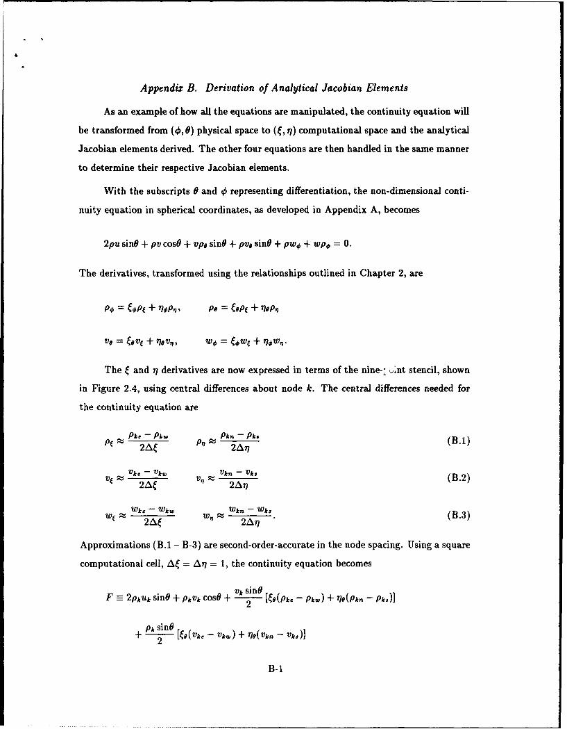
Appendix B. Derivation of Analytical Jacobian Elements

As an example of how all the equations are manipulated, the continuity equation will

be transformed from (4,, 6) physical space to (t, q) computational space and the analytical

Jacobian elements derived. The other four equations are then handled in the same manner

to determine their respective Jacobian elements.

With the subscripts 0 and 4, representing differentiation, the non-dimensional conti-

nuity equation in spherical coordinates, as developed in Appendix A, becomes

2pu sin0 + pv cos0 + vp. sin0 + pve sine + pw, + wpo = 0.

The derivatives, transformed using the relationships outlined in Chapter 2, are

PO = toP + '10P,7, Pe = GNPc + 77Pnp

ve = G•ov + 17OeV,, wO = Gw + 17,w,-

The ý and q derivatives are now expressed in terms of the nine-: '.nt stencil, shown

in Figure 2.4, using central differences about node k. The central differences needed for

the continuity equation are

PC cPk - Pkw " Pkn - Pk, (B.1)2AP 2Aq

vite - Vk, A Vkn - Vk, (B.2)• 2AC 2A?)

Wt;z e - wkw w n - Wks (B.3)

Approximations (B.1 - B-3) are second-order-accurate in the node spacing. Using a square

computational cell, Aý = A77= 1, the continuity equation becomes

F = 2pku sin + PVk coO+ V sin [G,(Pke - Pkw) + 770(Pkn - pk,)]

+ Pk sin2 [&I(vk- Vkw) + i7*(vk. - vk,)]2

B-1

"knw kn kne

kw k- ke

ksw "ks kse

Figure B.1 Nine-point Stencil for interior nodes

+kýw- [ - Wk,) + ,l#(Wkn - Wks)]

+ 'k- [ý#(Pk, - Pk.) + 77,(Pk. - Pk.)] = 0. (B.4)

The analytical Jacobian elements are now determined by taking partial derivatives

of (BA) with respect to each of the dicrete flow variables in the nine-point stencil, shown

in Figure B. 1. The Jacobian elements for the continuity equation are found to be

OF _ sinOOF = 2 uk sinG + Vk cosO + j [G(Vke- vk.) + 779(Vk. - Vk.)]ON 2

1+ 1 [C(#k(e - Wk.) + #,(Wkn - Wk,)],

OF _ Vh•G sinO WkCO OF OF

Ope = 2 + OPhN OPke'

OF vk 770 sinO Wk 70 OF OF-pn 2 -+ -2 ' p-k Opkna

OFS= 2pk sin&,OF _

OF = Pk cosO + sinO

OF PkGu sinO OF OF

Ovk• 2 OVk,, OVke

B-2

OF phn# sinf OF _OF

iiv-b - 2 ' 8vk. iiv-h

OF 1 [t (P.Ph + 17# (Pkn - Phe]

OF _Pkf# OF _OF

OýWk. 2 Tu'k. - Olki'

O F -phi?# OF _OF

Ow~ 2' jWe, - Wknj

B-3

Vita

Captain Larry K. Waters . He

graduated from Gull Lake High School in Richland, Michigan in 1978 and enlisted in

the United States Air Force on 4 May 1979. After serving as a computer operator and

programmer for six years, he was selected for the Airman Educational Commissioning

Program (AECP). He attended the University of Missouri-Rolla, where he graduated with

a Bachelor of Science in Aerospace Engineering in May 1988. He then attended Officer

Training School at Lackland AFB, Texas, where he was selected as First Honor Graduate

for class 88-12, for which he was awarded a regular commission. He then served four years

at the Phillips Laboratory, Kirtland AFB, New Mexico, where he worked on a variety of

high energy laser projects, until entering the School of Engineering, Air Force Institute of

Technology, in May 1992.

VITA- I

REPOT DCUMNTATON AGEForm ApprovedREPO T D CUME TATON P GE0MB No. 0704-0188

Pubitc rebo.crtin ourdenfa this' ý oiectton 'it fotmat'oh % estimlated to i''q - owrQ lesip~orw. mcttudirt the time to, e.-e.mg instructo~ns, searcn-ng ex-stng data soures~.gathering n mainta~tining the data needed. &no comoieting iri fen evvng t¶'e -. iC('ton ot n$orfnation Send commnents readn this burden estimate or Inv other aspect of thiscofiect,ao ot ntoynat~on. nclucmg s uggestions to( redu q -i ns orcen ic -V n "lnqro' ieadquarters Servces, O~renotrate f, nfrato Operations anla Reports, 12 1$ jetersonOaaisHihway, suite 1204. ArlingtOn,'JA 22202-4302. n Ir0 -e Otfceof Manaemnent and Suage. Paper~iiork Peoa lon P~cect ý074-0188). ~Vaihmtn9on, DX 20S03

1. AGENCY USE ONLY (Leave bln) 2REPORT DATE 3REPORT TYPE AND DATES COVERED

4. TITLE AND SUBTITLE 5. FUNDING NUMBERS

A NIHRICAL DEMO~1NTIEN (F B1RJUAT1K FOMNS RE LOW4 RE'ULDS04BER 0ICAL FUM

6. AUTHOR(S)

larry K. Wa~ters, Captain, LEAF

7. PERF^RMING ORGANIZATION NAME(S) AND ADDRESS(ES) B. PERFORMING ORGANIZATIONREPORT NUMBER

Air Force Institute of Technology, WPAFB Cif 45433-6583 AF]T/GAFV94Y/9¶)-29

9. SPONSORING/iMONITORING AGENCY NAME(S) AND ADORESS(ES) 10. SPONSORING/IMONITORINGAGENCY REPORT NUMBER

Dr D. BelkWright Laboratory, Armneit DirectorateEglin AFB, Florida 32542

11. SUPPLEMENTARY NOTES

:12a. DISTRIBUTION / AVAILABILITY STATEMENT 12b. DISTRIBUTION CODE

Approved for public release; distribuotion unlimited

113. A1BSTRACT (Meaximumn 200 words)It has long been established that supersonic flow over axisynnatric conical bodes at higangles of attack tend to develop a side force due to vortical asynuetry. (ne of the proposed

Ireasons for the aspmhtry is a bifurcation point in the solution of the Navier-Stokes equations.This study investigated the possible existence of a bifurcation. point :in the Navier-Stckesequations for subsonic laminar flow. Newton's method, with gaus elenination, uss usecL~to solvethe steady--state, viscous, canpressible Navier-Stioes equations :in spherical coordinatesasslining conical simiarty.

14. SUBJECT TERMS 15. NUMBER OF PAGES75

Navier-Stjkies, Viscous, Vortical Flow, Bifurcation, Newton's Method 16. PRICE CODE

17. SECURITY CLASSIFICATION 18. SECURITY CLASSIFICATION 19. SECURITY CLASSIFICATION 20. LIMITATION OF ABSTRACTOF REPORT OF THIS PAGE OF ABSTRACT

Unclassified Unclassified IUnclassified tILNSN 7540-01-280-5500 Standard Form 298 (Rev 2-89)

Prescribed by ANSI Stil Z39-18299- t02