Guyot et al 2013 - engit.monash.eduGuyot et al

© The Author 2013. Published by Oxford University Press. All rights reserved. For Permissions, please email: [email protected]

Tree Physiology 33, 187–194doi:10.1093/treephys/tps128

Using electrical resistivity tomography to differentiate sapwood from heartwood: application to conifers

Adrien Guyot1,2,3, Kasper T. Ostergaard2, Mothei Lenkopane1,2, Junliang Fan1,2 and David A. Lockington1,2

1National Centre for Groundwater Research and Training, Australia; 2School of Civil Engineering, The University of Queensland, St. Lucia 4072, Brisbane, Queensland, Australia; 3Corresponding author ([email protected])

Received May 24, 2012; accepted December 5, 2012; published online January 17, 2013; handling Editor David Whitehead

Estimating sapwood area is one of the main sources of error when upscaling point scale sap flow measurements to whole-tree water use. In this study, the potential use of electrical resistivity tomography (ERT) to determine the sapwood–heart-wood (SW–HW) boundary is investigated for Pinus elliottii Engelm var. elliottii × Pinus caribaea Morelet var. hondurensis growing in a subtropical climate. Specifically, this study investigates: (i) how electrical resistivity is correlated to either wood moisture content, or electrolyte concentration, or both, and (ii) how the SW–HW boundary is defined in terms of electrical resistivity. Tree cross-sections at breast height are analysed using ERT before being felled and the cross-section surface sampled for analysis of major electrolyte concentrations, wood moisture content and density. Electrical resistivity tomogra-phy results show patterns with high resistivities occurring in the inner part of the cross-section, with much lower values towards the outside. The high-resistivity areas were generally smaller than the low-resistivity areas. A comparison between ERT and actual SW area measured after felling shows a slope of the linear regression close to unity (=0.96) with a large spread of values (R2 = 0.56) mostly due to uncertainties in ERT. Electrolyte concentrations along sampled radial transects (cardinal directions) generally showed no trend from the centre of the tree to the bark. Wood moisture content and density show comparable trends that could explain the resistivity patterns. While this study indicates the potential for application of ERT for estimating SW area, it shows that there remains a need for refinement in locating the SW–HW boundary (e.g., by improvement of the inversion method, or perhaps electrode density) in order to increase the robustness of the method.

Keywords: conifers, electrolytes, electrical resistivity tomography, heartwood, sapwood, transpiration, wood moisture content.

Introduction

Tree water use estimates (Wullschleger et al. 1998) are not only significant to scientists but also to plantation managers and policy makers (Vanclay 2009). In Australia, the impact of pine tree plantations on catchment water balances has been recently noted (Zhang et al. 2011). Brown et al. (2007) have put for-ward a case for the need to improve our knowledge of planta-tion water use, which necessitates improving the accuracy of our estimation methods (Vanclay 2009). Furthermore, very few

studies (e.g., Dye et al. 1991, Bubb and Croton 2002) have investigated tropical pine tree water use and/or physiology, even though substantial variability in physiology (including larger sapwood (SW) width) has been observed for the species (Dye et al. 1991). While a number of methods exist for estimat-ing transpiration (at different scales), the use of direct measure-ments of sap flow using heat-based sensors is popular compared with the eddy-covariance technique and less demanding in terms of expertise. Estimating SW area is one of

Technical note

at UQ

Library on June 3, 2013http://treephys.oxfordjournals.org/

Dow

nloaded from

Tree Physiology Volume 33, 2013

the main sources of error when upscaling point sapflow mea-surements to tree transpiration (Hatton et al. 1995, Koestner et al. 1998, Clearwater et al. 1999). The SW–HW ratio is also of interest for commercial purposes, as SW will be used for paper production while heartwood (HW) volume is considered a wood productivity variable (Pereira et al. 2003). Several meth-ods have been proposed to determine the SW area, the most commonly used being coring the selected tree from a surface point towards the centre (Rust 1999), and determining the SW–HW boundary using an appropriate dye (Cermak et al. 1992). The radial thickness is converted to an area by rotation, assum-ing cross-sectional uniformity. Some authors have proposed a less invasive method where sap flow sensors with multiple thermistors along the needle are used to map the spatial vari-ability of sap flow across the stem (Cermak and Nadezhdina 1998). This method, however, is relatively time consuming and expensive for obtaining similar information to the coring method, but does additionally yield sap flow information. These methods provide very limited information about the cross-sectional area of the SW. The latter can be directly measured by injecting dye at the trunk base of a selective representative tree before felling and sampling the tree sections for the presence of dye (Umebayashi et al. 2010). However, it is clearly severely con-strained if estimates of SW area are required for a stand of trees. A fast, reliable and non- destructive method for measuring actual SW area for a number of trees in a stand would be extremely valuable for improving estimates of stand transpiration.

Recently, Hagrey (2006, 2007) demonstrated that electrical resistivity tomography (ERT) could be used to construct a spa-tial estimate of tree resistivity across the entire tree stem cross-section. Only a coarse resolution in the tomograph (~1–10 cm) was achieved in these studies. However, application of ERT is relatively fast and effectively non-destructive so poten-tially of value in estimating cross-sectional structure. While resistivity patterns can be due to the relative wetness of wood, they will also reflect patterns in electrolyte concentrations.

Wu et al. (2009) showed the potential use of ERT to map changes in stem moisture content over time in Populus trees. The ERT method has the advantage of being non-destructive, and relatively fast at a low cost. Recently, Bieker and Rust (2010a, 2010b), Bieker et al. (2010) and Brazee et al. (2010) experimented with ERT to determine fungal decay in tree stems, while Bieker and Rust (2010b) introduced the use of ERT to estimate SW and HW width in Pinus sylvestris L. They demonstrated the potential of this method, but highlighted some issues, namely: (i) low resistivity along the pith of P. syl-vestris and/or other conifers and (ii) the species’ specific inter-pretation of ERT signals (Bieker and Rust 2010a). Unfortunately, in their SW study, they did not conduct wood moisture content and density analyses and/or electrolyte concentrations as they did in their fungal decay study (Bieker and Rust 2010a). These

characteristics are potentially responsible for changes in resis-tivity across the stem (i.e., higher resistivities will be associ-ated with lower electrolytes concentration). Indeed, the SW–HW boundary could be mis-estimated if a strong gradient of elec-trolyte concentration occurs at the same boundary.

While potential for the method is indicated, there remains a lack of knowledge about: (i) how electrical resistivity is corre-lated to either wood moisture content, or electrolyte concen-tration, or both; and (ii) how well the SW–HW boundary can be defined in terms of electrical resistivity.

Thus, this study investigates: (i) how the measured electrical resistivity is related to wood moisture content or/and electro-lyte concentration, and subsequently (ii) the potential use of ERT to distinguish SW and HW. Our study is based on tropical pine tree species used widely in forestry in Southeast Queensland, Australia.

Materials and methods

Site description

The study was carried out in a pine plantation situated 60 km north of Brisbane in Queensland, Australia (26°57′13″S, 152°58′55″E). Trees in the plantation were 15-year-old Pinus elliottii Engelm var. elliottii × Pinus caribaea Morelet var. hondu-rensis with a mean canopy height of 16 m. The plantation stand density at the time of the study was ~450 trees per hectare.

In this study 10 trees from the same stand were randomly selected with circumferences ranging from 0.77 to 0.95 m (Table 1). Following the electrical resistivity measurements, the selected trees were felled in September 2011 and sampled for SW and moisture content analysis, as well as electrolyte analy-ses (aluminium (Al), calcium (Ca), iron (Fe), potassium (K), magnesium (Mg), sodium (Na), phosphorus (P) and sulphur (S)). Soil water content measurements were taken using time domain frequency probes on the day of the experiment in order to document its spatial variability and are shown in Table 1.

Electrical resistivity tomography

A multichannel, multielectrode resistivity system (Picus TreeTronic, Argus Electronic GmbH, Rostock, Germany) was used to perform the ERT using a dipole–dipole configuration (Daily and Ramirez 1995) at a low-frequency current of 8.3 Hz. For each of the measurements, several voltages (from 2 to 12 V) were applied to test the associated tomograph sensitiv-ity. Very slight (order of <0.5 % change) or no changes were observed when increasing the voltage, although low voltages led to insufficient electrical inputs.

Electrical resistivity tomography was performed on the selected trees on a clear, sunny and dry day following 2 weeks without any rainfall. As breast height (BH) is the common height used for sap flow measurements, ERT measurements were conducted at 1.5 m

188 Guyot et al.

at UQ


Dow

nloaded from

Tree Physiology Online at http://www.treephys.oxfordjournals.org

above the ground. For each tree, depending on the tree diameter, either 18 or 20 stainless-steel electrodes of 2 mm diameter and 30 mm length (Table 1) were inserted into the stemwood, evenly around the circumference with a 40–50 mm spacing. The stem-wood was identified by a change in resistance to electrode pene-tration, with penetration only being to a maximum depth of around a few millimetres. The ERT only requires that the electrodes are in contact with the moist wood. Bark was removed prior to insertion of the electrodes to improve electrical conductivity and prevent any interference in stem resistivity assessment that might be caused by extremely moist or dry bark. A digital calliper was used to measure the distance between the electrodes, and combined with the Picus Software to reconstruct a 2D spatial shape of the stem at that height.

Inversions were based on the acquired 2D shapes and the Picus Software (Picus TreeTronic, Argus Electronics GmbH), using a default smoothness of 20 and a maximal mesh fine-ness of 8. The inversion is based on algorithms by Guenther et al. (2006). Software outputs were processed using ArcGIS (ESRI 2011) and Scilab (Consortium Scilab 2011).

To check day-to-day variation, measurements were taken the day before and on the day of the experiment. In both cases, all 10 measurements were conducted within a 3-h timeframe.

Electrolyte concentration, wood moisture content and wood density

Trees were felled just after the electrical resistivity measure-ments were completed. Stem cross-sections in the plane of the tomography were photographed. The SW–HW boundary was determined based on the distinct colour change between the two (Prior et al. 2012). Additional microscopic analyses were carried out to confirm the SW–HW boundary. This SW depth is hereafter defined as the actual SW depth.

Sections of the trees at 1.5 m above the ground were taken to a field laboratory for sampling. Sap samples were taken following the same procedure as Isik and Li (2003). For the analysis of electrolyte concentration, sap was sampled for each

tree along an axis from the cambium to the HW, for each of the cardinal directions, at 10, 30, 50, 70 mm and at the centre of the tree stem (total of 170 samples).

Because of the rapid drying of the tree section after being cut, only trees 1, 2 and 4 were sampled for wood moisture content and wood density estimates. Vertical cores from the cross-sections were obtained as for the sap flow samples, using a 15 mm corer attached to a drill, and cored up to a depth of 30 mm. Samples were taken along the cambium to HW axis at 10, 30, 50, 70, 90 mm from the cambium, and at the centre of the stems for all cardinal directions for each of the three trees. These cylinders were sealed in the field, kept in ice and brought back to the laboratory where they were frozen and stored. For the analysis of electrolyte concentration, 50–150 mg of sap was digested with nitric acid in the laboratory, and ana-lysed by inductively coupled plasma-optical emission spectros-copy for Al, Ca, Fe, K, Mg, Na, P and S.

Samples were weighed (Wf) and then dried in an oven at 60 °C until there was no detectable change in their mass (after 16 days). Samples were weighed again (Wd). Wood moisture content (mc (g g−1)) was then determined as (Eq. (1))

m

W WWc

f d

d= −

(1)

Wood dry density ρd (g cm−3) was calculated as ρd = Wd/Vd, where Vd is the dry volume. Dry volume was determined fol-lowing the procedure described in Vandegehuchte and Steppe (2012).

Surface soil water content

Soil water content in the top 0.3 m was measured the day before the study using a portable time domain frequency probe (ICT international MP406, Armidale, Australia). Measurements consisted of three measurements of soil water content at 0.3, 0.6 and 0.9 m from the tree trunk taken at the four cardinal directions of each tree.

Tomographic differentiation of sapwood from heartwood 189

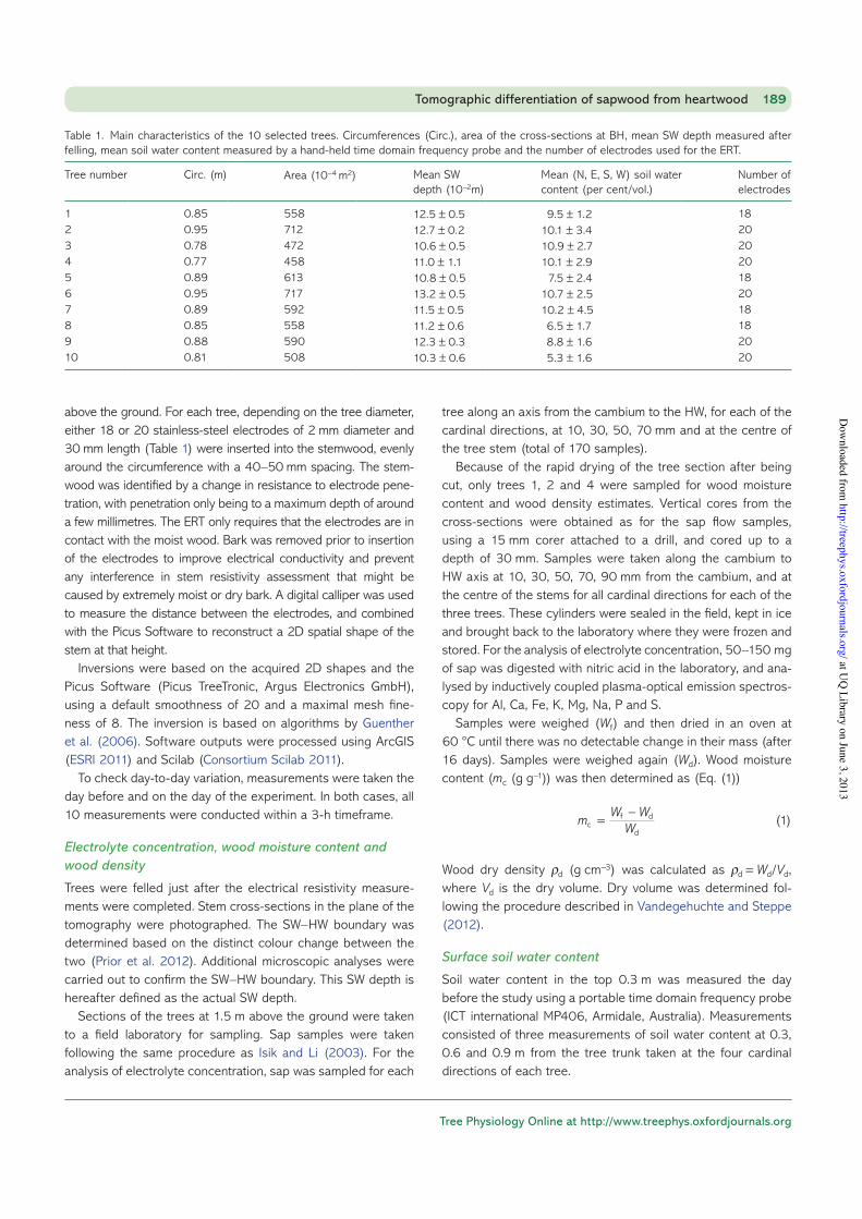
Table 1. Main characteristics of the 10 selected trees. Circumferences (Circ.), area of the cross-sections at BH, mean SW depth measured after felling, mean soil water content measured by a hand-held time domain frequency probe and the number of electrodes used for the ERT.

Tree number Circ. (m) Area (10−4 m2) Mean SW depth (10−2m)

Mean (N, E, S, W) soil water content (per cent/vol.)

Number of electrodes

1 0.85 558 12.5 ± 0.5 9.5 ± 1.2 182 0.95 712 12.7 ± 0.2 10.1 ± 3.4 203 0.78 472 10.6 ± 0.5 10.9 ± 2.7 204 0.77 458 11.0 ± 1.1 10.1 ± 2.9 205 0.89 613 10.8 ± 0.5 7.5 ± 2.4 186 0.95 717 13.2 ± 0.5 10.7 ± 2.5 207 0.89 592 11.5 ± 0.5 10.2 ± 4.5 188 0.85 558 11.2 ± 0.6 6.5 ± 1.7 189 0.88 590 12.3 ± 0.3 8.8 ± 1.6 2010 0.81 508 10.3 ± 0.6 5.3 ± 1.6 20

at UQ


Dow

nloaded from


Results

Electrical resistivity tomography

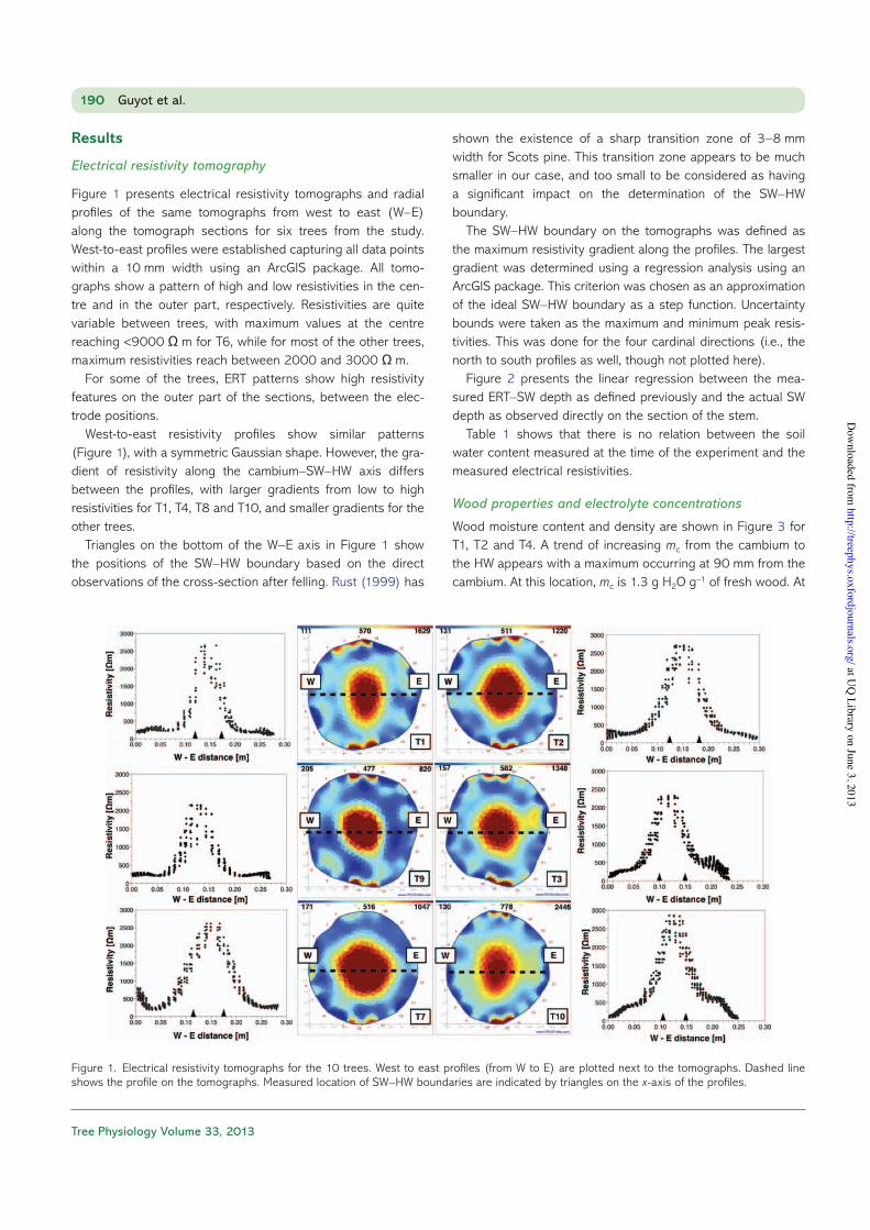
Figure 1 presents electrical resistivity tomographs and radial profiles of the same tomographs from west to east (W–E) along the tomograph sections for six trees from the study.West-to-east profiles were established capturing all data points within a 10 mm width using an ArcGIS package. All tomo-graphs show a pattern of high and low resistivities in the cen-tre and in the outer part, respectively. Resistivities are quite variable between trees, with maximum values at the centre reaching <9000 Ω m for T6, while for most of the other trees, maximum resistivities reach between 2000 and 3000 Ω m.

For some of the trees, ERT patterns show high resistivity features on the outer part of the sections, between the elec-trode positions.

West-to-east resistivity profiles show similar patterns (Figure 1), with a symmetric Gaussian shape. However, the gra-dient of resistivity along the cambium–SW–HW axis differs between the profiles, with larger gradients from low to high resistivities for T1, T4, T8 and T10, and smaller gradients for the other trees.

Triangles on the bottom of the W–E axis in Figure 1 show the positions of the SW–HW boundary based on the direct observations of the cross-section after felling. Rust (1999) has

shown the existence of a sharp transition zone of 3–8 mm width for Scots pine. This transition zone appears to be much smaller in our case, and too small to be considered as having a significant impact on the determination of the SW–HW boundary.

The SW–HW boundary on the tomographs was defined as the maximum resistivity gradient along the profiles. The largest gradient was determined using a regression analysis using an ArcGIS package. This criterion was chosen as an approximation of the ideal SW–HW boundary as a step function. Uncertainty bounds were taken as the maximum and minimum peak resis-tivities. This was done for the four cardinal directions (i.e., the north to south profiles as well, though not plotted here).

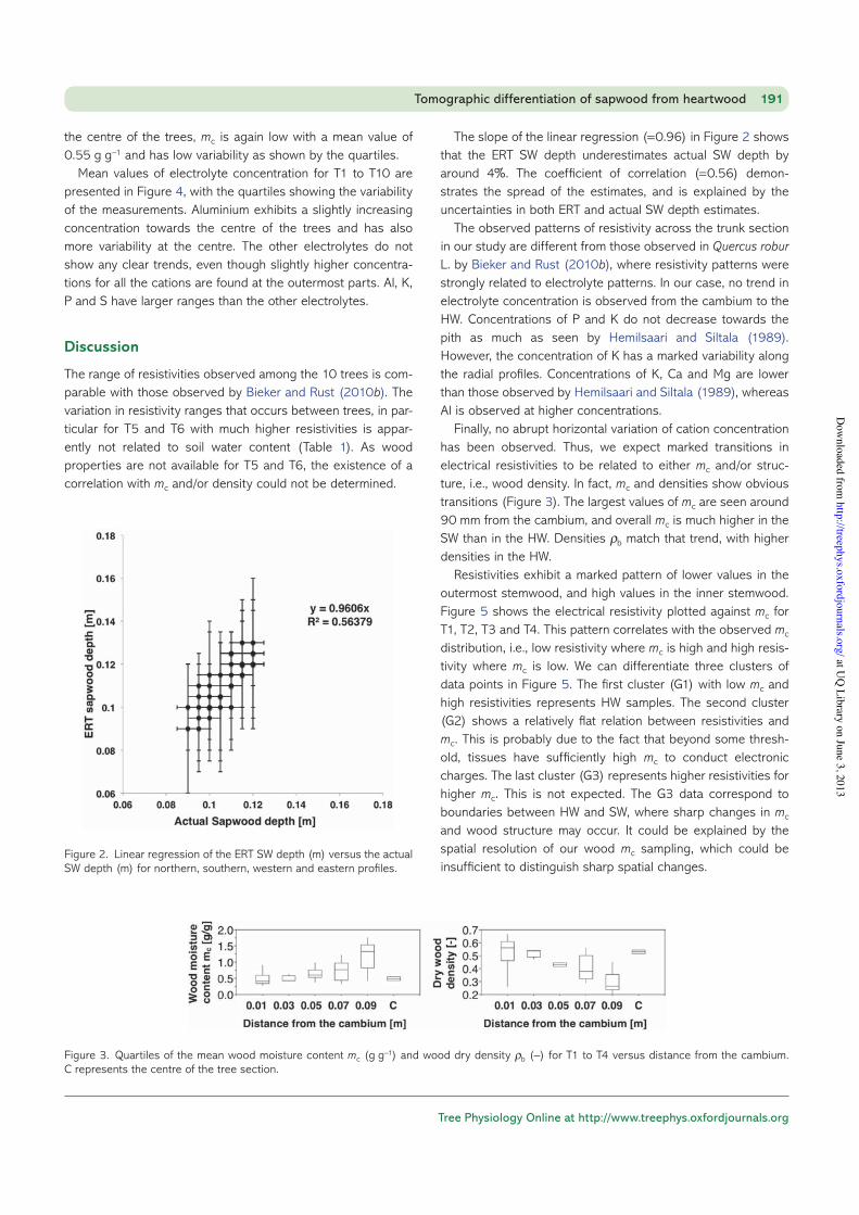
Figure 2 presents the linear regression between the mea-sured ERT–SW depth as defined previously and the actual SW depth as observed directly on the section of the stem.

Table 1 shows that there is no relation between the soil water content measured at the time of the experiment and the measured electrical resistivities.

Wood properties and electrolyte concentrations

Wood moisture content and density are shown in Figure 3 for T1, T2 and T4. A trend of increasing mc from the cambium to the HW appears with a maximum occurring at 90 mm from the cambium. At this location, mc is 1.3 g H2O g−1 of fresh wood. At

190 Guyot et al.

Figure 1. Electrical resistivity tomographs for the 10 trees. West to east profiles (from W to E) are plotted next to the tomographs. Dashed line shows the profile on the tomographs. Measured location of SW–HW boundaries are indicated by triangles on the x-axis of the profiles.

at UQ


Dow

nloaded from


the centre of the trees, mc is again low with a mean value of 0.55 g g−1 and has low variability as shown by the quartiles.

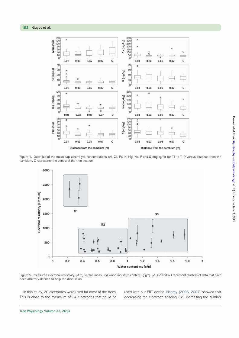
Mean values of electrolyte concentration for T1 to T10 are presented in Figure 4, with the quartiles showing the variability of the measurements. Aluminium exhibits a slightly increasing concentration towards the centre of the trees and has also more variability at the centre. The other electrolytes do not show any clear trends, even though slightly higher concentra-tions for all the cations are found at the outermost parts. Al, K, P and S have larger ranges than the other electrolytes.

Discussion

The range of resistivities observed among the 10 trees is com-parable with those observed by Bieker and Rust (2010b). The variation in resistivity ranges that occurs between trees, in par-ticular for T5 and T6 with much higher resistivities is appar-ently not related to soil water content (Table 1). As wood properties are not available for T5 and T6, the existence of a correlation with mc and/or density could not be determined.

The slope of the linear regression (=0.96) in Figure 2 shows that the ERT SW depth underestimates actual SW depth by around 4%. The coefficient of correlation (=0.56) demon-strates the spread of the estimates, and is explained by the uncertainties in both ERT and actual SW depth estimates.

The observed patterns of resistivity across the trunk section in our study are different from those observed in Quercus robur L. by Bieker and Rust (2010b), where resistivity patterns were strongly related to electrolyte patterns. In our case, no trend in electrolyte concentration is observed from the cambium to the HW. Concentrations of P and K do not decrease towards the pith as much as seen by Hemilsaari and Siltala (1989). However, the concentration of K has a marked variability along the radial profiles. Concentrations of K, Ca and Mg are lower than those observed by Hemilsaari and Siltala (1989), whereas Al is observed at higher concentrations.

Finally, no abrupt horizontal variation of cation concentration has been observed. Thus, we expect marked transitions in electrical resistivities to be related to either mc and/or struc-ture, i.e., wood density. In fact, mc and densities show obvious transitions (Figure 3). The largest values of mc are seen around 90 mm from the cambium, and overall mc is much higher in the SW than in the HW. Densities ρ b match that trend, with higher densities in the HW.

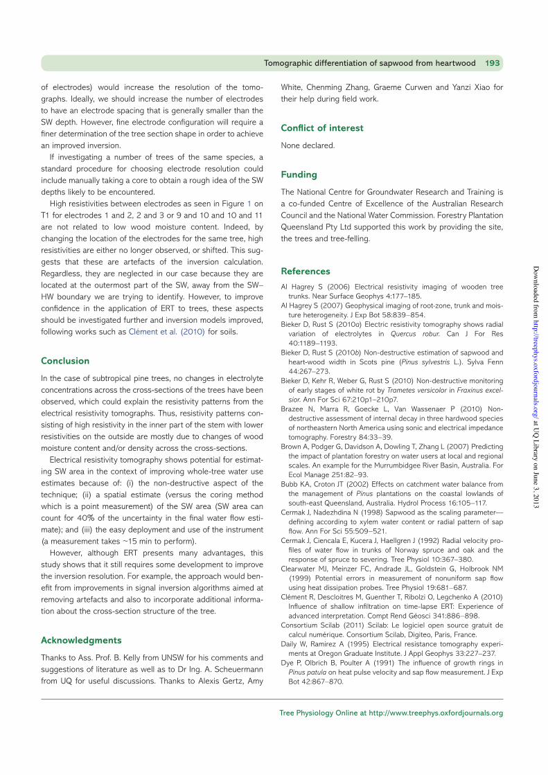
Resistivities exhibit a marked pattern of lower values in the outermost stemwood, and high values in the inner stemwood. Figure 5 shows the electrical resistivity plotted against mc for T1, T2, T3 and T4. This pattern correlates with the observed mc distribution, i.e., low resistivity where mc is high and high resis-tivity where mc is low. We can differentiate three clusters of data points in Figure 5. The first cluster (G1) with low mc and high resistivities represents HW samples. The second cluster (G2) shows a relatively flat relation between resistivities and mc. This is probably due to the fact that beyond some thresh-old, tissues have sufficiently high mc to conduct electronic charges. The last cluster (G3) represents higher resistivities for higher mc. This is not expected. The G3 data correspond to boundaries between HW and SW, where sharp changes in mc and wood structure may occur. It could be explained by the spatial resolution of our wood mc sampling, which could be insufficient to distinguish sharp spatial changes.


Figure 2. Linear regression of the ERT SW depth (m) versus the actual SW depth (m) for northern, southern, western and eastern profiles.

Figure 3. Quartiles of the mean wood moisture content mc (g g−1) and wood dry density ρ b (−) for T1 to T4 versus distance from the cambium. C represents the centre of the tree section.

at UQ


Dow

nloaded from


In this study, 20 electrodes were used for most of the trees. This is close to the maximum of 24 electrodes that could be

used with our ERT device. Hagrey (2006, 2007) showed that decreasing the electrode spacing (i.e., increasing the number

192 Guyot et al.

Figure 5. Measured electrical resistivity (Ω m) versus measured wood moisture content (g g−1). G1, G2 and G3 represent clusters of data that have been arbitrary defined to help the discussion.

Figure 4. Quartiles of the mean sap electrolyte concentrations (Al, Ca, Fe, K, Mg, Na, P and S (mg kg−1)) for T1 to T10 versus distance from the cambium. C represents the centre of the tree section.

at UQ


Dow

nloaded from


of electrodes) would increase the resolution of the tomo-graphs. Ideally, we should increase the number of electrodes to have an electrode spacing that is generally smaller than the SW depth. However, fine electrode configuration will require a finer determination of the tree section shape in order to achieve an improved inversion.

If investigating a number of trees of the same species, a standard procedure for choosing electrode resolution could include manually taking a core to obtain a rough idea of the SW depths likely to be encountered.

High resistivities between electrodes as seen in Figure 1 on T1 for electrodes 1 and 2, 2 and 3 or 9 and 10 and 10 and 11 are not related to low wood moisture content. Indeed, by changing the location of the electrodes for the same tree, high resistivities are either no longer observed, or shifted. This sug-gests that these are artefacts of the inversion calculation. Regardless, they are neglected in our case because they are located at the outermost part of the SW, away from the SW–HW boundary we are trying to identify. However, to improve confidence in the application of ERT to trees, these aspects should be investigated further and inversion models improved, following works such as Clément et al. (2010) for soils.

Conclusion

In the case of subtropical pine trees, no changes in electrolyte concentrations across the cross-sections of the trees have been observed, which could explain the resistivity patterns from the electrical resistivity tomographs. Thus, resistivity patterns con-sisting of high resistivity in the inner part of the stem with lower resistivities on the outside are mostly due to changes of wood moisture content and/or density across the cross-sections.

Electrical resistivity tomography shows potential for estimat-ing SW area in the context of improving whole-tree water use estimates because of: (i) the non-destructive aspect of the technique; (ii) a spatial estimate (versus the coring method which is a point measurement) of the SW area (SW area can count for 40% of the uncertainty in the final water flow esti-mate); and (iii) the easy deployment and use of the instrument (a measurement takes ~15 min to perform).

However, although ERT presents many advantages, this study shows that it still requires some development to improve the inversion resolution. For example, the approach would ben-efit from improvements in signal inversion algorithms aimed at removing artefacts and also to incorporate additional informa-tion about the cross-section structure of the tree.

Acknowledgments

Thanks to Ass. Prof. B. Kelly from UNSW for his comments and suggestions of literature as well as to Dr Ing. A. Scheuermann from UQ for useful discussions. Thanks to Alexis Gertz, Amy

White, Chenming Zhang, Graeme Curwen and Yanzi Xiao for their help during field work.

Conflict of interest

None declared.

Funding

The National Centre for Groundwater Research and Training is a co-funded Centre of Excellence of the Australian Research Council and the National Water Commission. Forestry Plantation Queensland Pty Ltd supported this work by providing the site, the trees and tree-felling.

References

Al Hagrey S (2006) Electrical resistivity imaging of wooden tree trunks. Near Surface Geophys 4:177–185.

Al Hagrey S (2007) Geophysical imaging of root-zone, trunk and mois-ture heterogeneity. J Exp Bot 58:839–854.

Bieker D, Rust S (2010a) Electric resistivity tomography shows radial variation of electrolytes in Quercus robur. Can J For Res 40:1189–1193.

Bieker D, Rust S (2010b) Non-destructive estimation of sapwood and heart-wood width in Scots pine (Pinus sylvestris L.). Sylva Fenn 44:267–273.

Bieker D, Kehr R, Weber G, Rust S (2010) Non-destructive monitoring of early stages of white rot by Trametes versicolor in Fraxinus excel-sior. Ann For Sci 67:210p1–210p7.

Brazee N, Marra R, Goecke L, Van Wassenaer P (2010) Non-destructive assessment of internal decay in three hardwood species of northeastern North America using sonic and electrical impedance tomography. Forestry 84:33–39.

Brown A, Podger G, Davidson A, Dowling T, Zhang L (2007) Predicting the impact of plantation forestry on water users at local and regional scales. An example for the Murrumbidgee River Basin, Australia. For Ecol Manage 251:82–93.

Bubb KA, Croton JT (2002) Effects on catchment water balance from the management of Pinus plantations on the coastal lowlands of south-east Queensland, Australia. Hydrol Process 16:105–117.

Cermak J, Nadezhdina N (1998) Sapwood as the scaling parameter—defining according to xylem water content or radial pattern of sap flow. Ann For Sci 55:509–521.

Cermak J, Ciencala E, Kucera J, Haellgren J (1992) Radial velocity pro-files of water flow in trunks of Norway spruce and oak and the response of spruce to severing. Tree Physiol 10:367–380.

Clearwater MJ, Meinzer FC, Andrade JL, Goldstein G, Holbrook NM (1999) Potential errors in measurement of nonuniform sap flow using heat dissipation probes. Tree Physiol 19:681–687.

Clément R, Descloitres M, Guenther T, Ribolzi O, Legchenko A (2010) Influence of shallow infiltration on time-lapse ERT: Experience of advanced interpretation. Compt Rend Géosci 341:886–898.

Consortium Scilab (2011) Scilab: Le logiciel open source gratuit de calcul numérique. Consortium Scilab, Digiteo, Paris, France.

Daily W, Ramirez A (1995) Electrical resistance tomography experi-ments at Oregon Graduate Institute. J Appl Geophys 33:227–237.

Dye P, Olbrich B, Poulter A (1991) The influence of growth rings in Pinus patula on heat pulse velocity and sap flow measurement. J Exp Bot 42:867–870.


at UQ


Dow

nloaded from


ESRI (2011) ArcGIS desktop: Release 10. Environmental Systems Research Institute, Redlands, CA.

Guenther T, Ruecker C, Spitzer K (2006) Three-dimensional modelling and inversion of DC resistivity data incorporating topography—II. Inversion. Geophys J Int 166:506–517.

Hatton TJ, Moore SJ, Reece PH (1995) Estimating stand transpiration in Eucalyptus populnea woodland with the heat pulse method: measure-ments errors and sampling strategies. Tree Physiol 14:219–227.

Hemilsaari HS, Siltala T (1989) Variations in nutrient concentrations of Pinus sylvestris stems. Scand J For Res 4:1–4, 443–451.

Isik F, Li B (2003) Rapid assessment of wood density of live trees using the Resistograph for selection in tree improvement programs. Can J For Res 33:2426–2435.

Koestner B, Granier A, Cermak J (1998) Sapflow measurements in for-est stands: methods and uncertainties. Ann For Sci 55:13–27.

Pereira H, Graca J, Rodrigues JC (2003) Wood chemistry in relation to quality. In: Barnett JR, Jeronimidis G (eds) Wood quality and its biologi-cal basis. CRC Press and Blackwell Publishing, Oxford, UK, pp 53–83.

Prior L, Brodribb TJ, Tng DYP, Bowman MJS (2012) From desert to rainforest, sapwood width is similar in the widespread

conifer Callitris columellaris. Trees Struct Funct doi:10.1007/s00468-012-0779-3.

Rust S (1999) Comparison of three methods for determining the conduc-tive xylem area of Scots pine (Pinus sylvestris). Forestry 72:103–108.

Umebayashi T, Utsumi Y, Koga S, Inoue S et al. (2010) Xylem water-con-ducting patterns of 34 broadleaved evergreen trees in southern Japan. Trees 24:571–583.

Vanclay KJ (2009) Managing water use from forest plantations. For Ecol Manage 257:385–389.

Vandegehuchte MW, Steppe K (2012) Improving sap flux density mea-surements by correctly determining thermal diffusivity, differentiat-ing between bound and unbound water. Tree Physiol 32:930–942.

Wu H, Zhou Q, Liu H, Tang M (2009) Application of electrical resistiv-ity tomography in studying water uptake process in tree trunk. Chin J Ecol 28:350–356.

Wullschleger S, Meinzer F, Vertessy R (1998) A review of whole plant water use studies in trees. Tree Physiol 18:499–512.

Zhang L, Zhao F, Chen Y, Dixon RNM (2011) Estimating effects of plantation expansion and climate variability on streamflow for catch-ments in Australia. Water Resour Res 47:W12539.

194 Guyot et al.

at UQ


Dow

nloaded from

Documents

Guyot et al 2013 - engit.monash.eduGuyot et al