Embed Size (px)
Citation preview
,~L COPY APu. .9o- o hII,,j"
cv3 DYNAMIC FRACTURE OF CONCRETE
00 PART I
l ~~~~~~~Jiaji Du <: .. ",-, ,,Department of Mechanical Engineering ,+ . .
A.S. Kobayashi :+ ,.Department of Mechanical Engineering
DTIC + ,E LE CTIE Neil M. Hawkins .,"Department of CM il EngineeringIE.ET Onei . Hawki+ns"FEB 2 3 1990DeatetoCIEniergI') University of Washington
Seattle, WA 98195
.. . ......... ,,: -
'3
z
Prepared for
Air Force Office of Scientific ResearchBoiling Air Force BaseWashington, DC 20332-6448
Final Report on AFOSR Contract 86-0204
February 14, 1990
I Distribution Unlimited: I
90 02 23 081
Unclassified-- SECURITY CLASIFICATION OF THIS PAGE
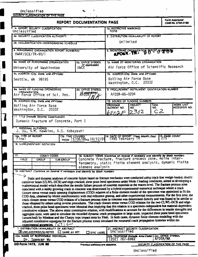
" Form ApprovedUIasREPORT DOCUMENTATION PAGE OMUNO.0704-088
'a. REPORT SECURITY CLASSIFICATION lb RESTRICTIVE MARKINGSUnclassified None2a. SECURITY CLASSIFICATION AUTHORITY 3. DISTRIBUTION/AVAILABILITY OF REPORT
2b. DECLASSIFICATION / DOWNGRADING SCHEDULE Un li mi ted
PERFORMING ORGANIZATION REPORT NUMBER(S) S. MONITORING OR I TIO RUWAF/DCE/TR-90/I o rwt -IyulK,
6a. NAME OF PERFORMING ORGANIZATION 6b. OFFICE SYMBOL 7a. NAME OF MONITORING ORGANIZATION
University of Washinaton UW i appl cab e) Air Force Office of Scientific Research
6c. ADDRESS (City, State, and ZIP Code) 7b. ADDRESS (City, State, and ZIP Code)
Seattle, WA 98195 Bolling Air Force BaseWashington, D.C. 20332
Ba. NAME OF FUNDING/SPONSORING 8b. OFFICE SYMBOL 9. PROCUREMENT INSTRUMENT IDENTIFICATION NUMBERORGANIZATION AFOSR-(86-t2
Air Force Office of Sci. Res. AFOSR-86-0204
87c. ADDRESS (City, State, and ZIPCode) 10. SOURCE OF FUNDING NUMBERS
Bolling Air Force Base PROGRAM PROJECT TASK IWORK UNITWashington, D.C. 20332 ELEMENT NO. NO NO. IACCESSION NO.
11. TITLE (Include Securty Classification)
Dynamic Fracture of Concrete, Part I
" PERSONAL AUTHOR(S)J. Du, N.M. Hawkins, A.S. Kobayashi
13a. TYPE OF REPORT 1b. TIME COVERED 4/2814. DATE OF REPORT (Yef4, Month, Day)CONFinal I FROM 15/0 6/8 6rO 4/12/8 1990 February IU
16. SUPPLEMENTARY NOTATION
17. COSATI CODES 18. SUBJECT TERMS (Continue on reverse if necessary and identify by block number)FIELD GROUP SUB-GROUP Concrete fracture, fracture process zone, moire inter-
ferometry, static finite element analysis, dynamic finiteelement analysis
19. ABSTRACT (Continue on reverie if necessary and identify by block number)
Static and dynamic analyses of concrete failure based on fracture mechanics were conducted using crack-line wedge-load , doublecantilever beam (CLWL-DCB) and edge-cracked, three point bend specimens under Mode I loading conditions, aimed at developing amathematical model which describes the tensile failure process of concrete materials at the macro-level. The fractm process zoneassociated with a stably growing crack in concrete was determined by a hybrid experimental-numerical technique where a crackclosure stress versus crack opening displacement (COD) relation of a finite element model of the specimen was optimized to fit theCOD data, obtained by Moire interferometry with real reference grating, and other experimental measurements. For the first time, thecrack closure stres versus COD relation of a fracture process zone in concrete was determined directly and was fomd to be similar tothose obtained by others using inverse procedures. The crack closure stres versus COD relation for the two CLWL-DCB and edge-cracked, three point bend specimens were identical thus implying that this relation is a specimen-independent but material-dependentconstitutive relation. The above static constitutive relation, with modifications to account for the differences in tensile strengths andaggregate sizes, were used to simulate the recorded dynamic crack propagaton in large scale, impacted three point bend specimens(unnotched) by Mindess and the Charpy type impact tests by Shah. In both cases, dynamic finite element modeling with theadjusted constitutive equavm for the fracture process zones simulated the measured crack propagation histories within the
I. DISTRIBUTION /AVAILABILITY OF ABSTRACT 21. AB)TRACT SECURITY CLASSIFICATION13UNCLASSIFIEDUNLIMITED C SAME AS RPT. Q TIC USERS, Uncassified
22&. NAME OF RESPONSIBLE INDIVIDUAL 2t b. TEL EPHONIE (kincude AWga Code) 22c. OFFICE SYMBOL
Dr. Spencer Wu (202) 767-6962 AFOSR/NADD Form 1473, JUN 86 Pre vious e ons are obsolete. SECURITY CLASSIFICATION OF THIS PAGE
Unclassified

ft)
Research sponsored by the Air Force Office of ScientificResearch, Air Force Systems Command, USAF, under grantor cooperative agreement number, AFOSR XX-XXXX. The USGovernment is authorized to reproduce and distributereprints for Governmental purposes notwithstanding anycopyright notation thereon.
This manuscript is submitted for publication with theunderstanding that the US Government is authorized toreproduce and distribute reprints for Governmentalpurposes.
Abstract
Static and dynamic analyses of concrete failure
based on fracture mechanics were conducted using
crack-line wedge-loaded, double cantilever beam
(CLWL-DCB) and edge-cracked, three point bend
specimens under Mode I loading conditions, aimed at
developing a mathematical model which describes the
tensile failure process of concrete materials at the
macro-level.
The fracture process zone associated with a
stably growing crack in concrete was determined by a
hybrid experimental-numerical technique where a
crack closure stress versus crack opening
displacement (COD) relation of a finite element
model of the specimen was optimized to fit the COD
data, obtained by Moire interferometry with real
reference grating, and other experimental
measurements.
For the first time, the crack closure stress
versus COD relation of a fracture process zone in
concrete was determined directly and was found to be
similar to those obtained by others using inverse
procedures. The crack closure stress versus COD
relation for the two CLWL-DCB and edge-cracked,
three point bend specimens were identical thus
implying that this relation is a specimen-
independent but material-dependent constitutive
relation.
The above static constitutive relation, with
modifications to account for the differences in
tensile strengths and aggregate sizes, were used to
simulate the recorded dynamic crack propagation in
large scale, impacted three point bend specimens
(unnotched) by Mindess and the Charpy type impact
tests by Shah. In both cases, dynamic finite
element modeling with the adjusted constitutive
equations for the fracture process zones simulated
the measured crack propagation histories within the
experimental accuracies.
JS,:'_ CF.A&l
L..C ... ..
. . .. ... ,..
, - -- :I 0D., I .
~iL~.]
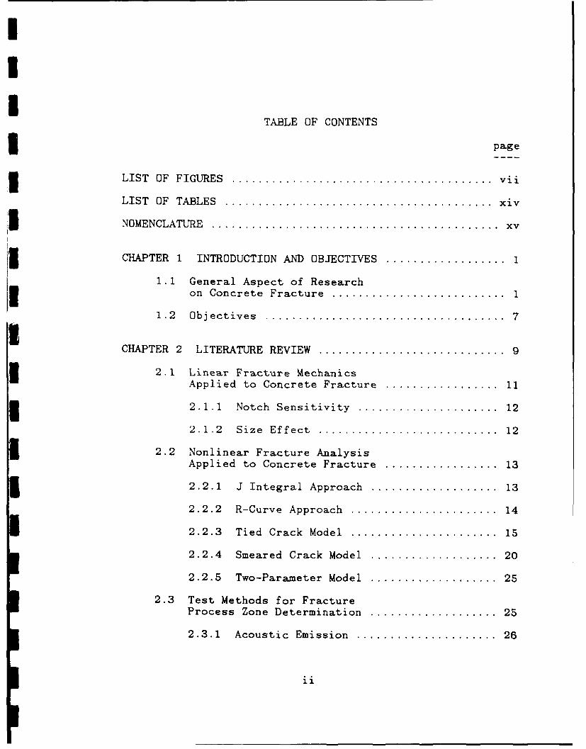
TABLE OF CONTENTS
page
LIST OF FIGURES ....................................... vii
LIST OF TABLES ........................................ xiv
NOMENCLATURE ........................................... xv
CHAPTER 1 INTRODUCTION AND OBJECTIVES .................... 1
1.1 General Aspect of Researchon Concrete Fracture ............................ 1
1 .2 Objectives .................................... 7
CHAPTER 2 LITERATURE REVIEW ............................ 9
2.1 Linear Fracture MechanicsApplied to Concrete Fracture .................. 11
2.1.1 Notch Sensitivity ....................... 12
2.1.2 Size Effect ........................... 12
2.2 Nonlinear Fracture AnalysisApplied to Concrete Fracture .................. 13
2.2.1 J Integral Approach ..................... 13
2.2.2 R-Curve Approach ........................ 14
2.2.3 Tied Crack Model ........................ 15
2.2.4 Smeared Crack Model .................... 20
2.2.5 Two-Parameter Model ..................... 25
2.3 Test Methods for FractureProcess Zone Determination ..................... 25
2.3.1 Acoustic Emission ....................... 26
ii
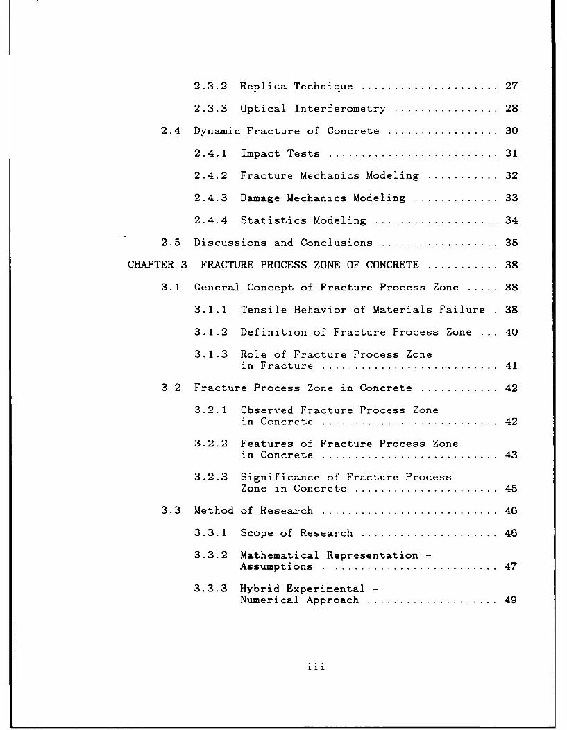
2.3.2 Replica Technique ..................... 27
2.3.3 Optical Interferometry ................. 28
2.4 Dynamic Fracture of Concrete ................... 30
2.4.1 Impact Tests .......................... 31
2.4.2 Fracture Mechanics Modeling ............ 32
2.4.3 Damage Mechanics Modeling .............. 33
2.4.4 Statistics Modeling ..................... 34
2.5 Discussions and Conclusions .................... 35
CHAPTER 3 FRACTURE PROCESS ZONE OF CONCRETE ............ 38
3.1 General Concept of Fracture Process Zone ..... 38
3.1.1 Tensile Behavior of Materials Failure . 38
3.1.2 Definition of Fracture Process Zone ... 40
3.1.3 Role of Fracture Process Zonein Fracture ........................... 41
3.2 Fracture Process Zone in Concrete ............. 42
3.2.1 Observed Fracture Process Zonein Concrete ........................... 42
3.2.2 Features of Fracture Process Zonein Concrete ........................... 43
3.2.3 Significance of Fracture ProcessZone in Concrete ...................... 45
3.3 Method of Research ........................... 46
3.3.1 Scope of Research ..................... 46
3.3.2 Mathematical Representation -Assumptions ........................... 47
3.3.3 Hybrid Experimental -Numerical Approach .................... 49
iii
CHAPTER 4 EXPERIMENTAL APPROACH ....................... 51
4.1 Test Program ................................. 51
4.1.1 Objectives of the Experiments ......... 51
4.1.2 Test Groups and Test Variables ........ 52
4.1.3 Loading and Data Recording Devices .... 56
4.2 Specimen Preparation ......................... 58
4.2.1 Fabrication of Specimens ............... 58
4.2.2 Material Properties Determination ..... 60
4.2.3 Specimen Surface Treatmentfor Moire Testing ....................... 62
4.3 Moire Interferometry Test Method .............. 63
4.3.1 Introduction to MoireInterferometry Method ................... 63
4.3.2 Moire Interferometrywith Real Reference Grating ............ 68
4.3.3 Moire Interferometrywith White Light ...................... 71
4.4 Optical Instrumentationand Test Procedures .......................... 73
4.4.1 White Light Moire Set-Up ............... 73
4.4.2 Laser Moire Set-Up ...................... 74
4.4.3 Test Procedures ....................... 77
CHAPTER 5 NUMERICAL PROCEDURES .......................... 81
5.1 Finite Element Analysis ...................... 81
5.1.1 Special Featuresin Finite Element Analysis ............. 81
5.1.2 Superposition Principleand Fundamental Solutions .............. 85
iv
5.1.3 FormulationUsing Fundamental Solutions ............ 86
5.2 Indirect Method .............................. 89
5.2.1 Three - Line Model .................... 89
5.2.2 Iteration Simulation Scheme ............ 92
5.2.3 Trial and Error Procedure .............. 93
5.3 Direct Method ................................ 93
5.3.1 Motivations ........................... 93
5.3.2 One - Curve Model ..................... 96
5.3.3 Optimization Procedure .................. 99
5.4 Discussion on Numerical Procedure ............ 101
5.4.1 Prediction of Crack Propagation ...... 101
5.4.2 Relation between Indirect andDirect Methods ....................... 102
5.4.3 Finite Element Size .................... 103
CHAPTER 6 STATIC FRACTURE OF CONCRETE SPECIMENS ...... 104
6.1 Small Three Point Bend Specimens ............. 104
6.1.1 Experimental Results ................... 104
6.1.2 Numerical Results .................... 113
6.2 Large Double Cantilever Beam Specimens ...... 116
6.2.1 Experimental Results ................... 118
6.2.2 Numerical Results .................... 127
6.3 Specimens of Adequate Size .................... 127
6.3.1 Experimental Results ................... 131
6.3.2 Numerical Results .................... 145
v
6.3.3 Discussions .......................... 155
CHAPTER 7 DYNAMIC FRACTURE OF CONCRETE SPECIMENS ..... 163
7.1 Dynamic Fracture Process Zone Model ......... 163
7.1.1 General . .............................. 162
7.1.2 Formulation Considerations ........... 164
7.2 Preliminary Results ......................... 165
7.2.1 Simulation of Mindess' Impact Tests .. 165
7.3 Refined Results ............................. 187
7.3.1 Simulation of Shah' Impact Tests ..... 187
CHAPTER 8 SUMMARY . .................................... 211
CHAPTER 9 CONCLUSIONS ................................ 218
CHAPTER 10 RECOMMENDATIONS ........................... 220
REFERENCES . ............................................ 223
APPENDIX A DETAILS OF SPECIMEN PREPARATION ........... 236
APPENDIX B FABRICATION AND TRANSFERDIFFRACTION GRATING ....................... 239
APPENDIX C SOLUTION OF OVERDETERMINISTICEQUATIONS ................................. 243
APPENDIX D SOME DYNAMIC FINITE ELEMENTCOMPUTATION DETAILS ....................... 245
APPENDIX E A MODEL FOR FATIGUE OF
A SIMILAR MATERIAL ........................ 251
APPENDIX F KR CURVE RE-EVALUATION
BASED ON TEST RESULTS ..................... 267
I vi
II
LIST OF FIGURES Ipage
Figure 3.1 Comparison of Tensile Behavior ofMetal and Concrete ........................... 39
Figure 3.2 Normal Stress Distribution AroundFracture Process Zone ....................... 44
Figure 3.3 Published Direct Tension Test Results ...... 48 5Figure 4.1 Small Beam and Large CLWL-DCB Specimens
(a) Group 1, (b) Group 2,3 .................. 54
Figure 4.2 Specimens of Appropriate Sizes(a) Group 4, (b) Group 5 .................... 55 1
Figure 4.3 Wedge Load and Specimen Holding Assemblyfor CLWL-DCB Specimen Tests Group 2,3,4 .... 57 3
Figure 4.4 Principle of Moire Interferometry .......... 65
Figure 4.5 Generation of Virtual Grating withReal Reference Grating ...................... 70
Figure 4.6 Optical Set-Up for White Light MoireInterferometry (f=1200 lines/mm) ........... 72
Figure 4.7 Optical Set-UP for Laser MoireInterferometry (f=1200 lines/mm) ........... 75 I
Figure 4.8 Staging for Real Reference Grating ......... 78
Figure 5.1 Boundary Conditions and Loading Systems .... 83
Figure 5.2 Fracture Process Zone Modelwith Three Line Segments .................... 91
Figure 5.3 Assumed Functional Form for CrackClosure Stress Versus COD Relation ......... 98
Figure 6.1 Experimental Set-Up for Test Group 1 ....... 105
Figure 6.2 Moire Interferometric Pattern at Crack Tip
Three Point Bend Specimen No. SB-iat Load 624 N ................................ 107 5
vii i
I
Figure 6.3 Moire Interferometric Pattern at Crack TipThree Point Bend Specimen No. SB-4at Load 557 N ............................... 108
Figure 6.4 COD Variations along Fracture Process ZoneSpecimen No. SB-1 ........................... 109
Figure 6.5 COD Variations along Fracture Process ZoneSpecimen No. SB-4 ........................... 110
Figure 6.6 COD at Prenotch End Versus Microcrack ExtensionSmall Three Point Bend Specimen ........... 112
Figure 6.7 Finite Element Model of the ConcreteSmall Three Point Bend Specimen ........... 114
Figure 6.8 Crack Closure Stress Versus COD Relationfor Concrete Fracture Process ZoneGroup 1. Small Beams ...................... 115
Figure 6.9 Load Vesus Crack Mouth Opening Displacementfor Small Three Point Bend Specimens ...... 117
Figure 6.10 Experimental Set-Up for Test Group 2,3. .. 119
Figure 6.11 Wedge Load Versus 2V 1 for Large CLWL-DCB
Specimens No. LD-1 and No. LD-2 ........... 120
Figure 6.12 Wedge Load Versus 2V1 for Large CLWL-DCB
Specimens No. LD-3 and No. LD-4 .......... 121
Figure 6.13 2V 2 Versus 2V I for Large CLWL-DCB
U Specimens No. LD-1 and No. LD-2 .......... 122
Figure 6.14 2V 2 Versus 2V 1 for Large CLWL-DCB
Specimens No. LD-3 and No. LD-4 ........... 123
Figure 6.15 COD Variations along Fracture Process ZoneSpecimen No. LD-1 .......................... 125
Figure 6.16 COD Variations along Fracture Process ZoneSpecimen No. LD-3 .......................... 126
Figure 6.17 Finite Element Mesh for Group 2,3.Large CLWL-DCB Specimens .................. 128
viii
Figure 6.18 Crack Closure Stress Versus COD Relationfor Group 2 Specimens ...................... 129
Figure 6.19 Crack Closure Stress Versus COD Relationfor Group 3 Specimens ...................... 130
Figure 6.20 Experimental Set-Up for Test Group 4...... 132
Figure 6.21 Optical Set-Up for Laser Beam ............. 133
Figure 6.22 Experimental Set-Up for Test Group 5...... 134
Figure 6.23 Wedge Load Versus 2V1 for Small
CLWL-DCB Specimens, Group 4 ............... 135
Figure 6.24 2V 2 Versus 2V1 for Small
CLWL-DCB Specimens, Group 4 ............... 136
Figure 6.25 Load Versus Deflection Curves forThree Point Bend Specimens, Group 5 ....... 137
Figure 6.26 Sequential Moire Fringe Patterns ofCLWL-DCB Specimen, Specimen No. SD-2 ..... 139
Figure 6.27 Sequential Moire Fringe Patterns of ThreePoint Bend Specimen, Specimen No. LB-i ... 140
Figure 6.28 COD Variations along Fracture Process ZoneCLWL-DCB Specimen No. SD-2 ................ 141
Figure 6.29 COD Variations along Fracture Process ZoneCLW L-DCB Specimen No. SD-4 ................ 142
Figure 6.30 COD Variations along Fracture Process ZoneThree Point Bend Specimen No. LB-4 ....... 143
Figure 6.31 COD Variations along Fracture Process ZoneThree Point Bend Specimen No. LB-i ....... 144
Figure 6.32 Finite Element Mesh for Group 4Small CLWL-DCB Specimens ................... 146
Figure 6.33 Finite Element Mesh for Group 5Large Three Point Bend Specimens .......... 147
Figure 6.34 Crack Closure Stress Versus COD Relationfor One Continuous Curve Model ............ 149
ix
Figure 6.35 Comparison of Crack Closure Stress VersusCOD Relationship with Published DirectTension Test Results ..................... 150
Figure 6.36 Comparison of Three - Line Model withOne - Curve Model for Group 4,5 specimens 151
Figure 6.37 Comparison of Test and NumericallyGenerated Moire Fringe Patterns.CLWL-DCB Specimen No. SD-4 ................. 153
Figure 6.38 Comparison of Test and NumericallyGenerated Moire Fringe Patterns.Three Point Bend Specimen No. LB-I ....... 154
Figure 6.39 Computed Sequential Normal StressDistributions along the Crack Pathin Group 4 CLWL-DCB Specimens ............. 156
Figure 6.40 Computed Sequential Normal StressDistributions along the Crack Pathin Group 5 Three Point Bend Specimens .... 157
Figure 6.41 Energy Partition for Small CLWL-DCBSpecimen, Group 4 ........................ 158
Figure 6.42 Energy Partition for Large Three Point BendSpecimen, Group 5 ........................ 159
Figure 6.43 Crack closure stress, Crack OpeningDisplacement Distributions alongFracture Process Zone and AsociatedComputed Moire Fringe Pattern forCLWL-DCB Specimen No. SD-4 ................. 162
Figure 7.1 Fracture Process Zone of Concretefor Dynamic Fracture Modelling ............. 166
Figure 7.2 Crack Closure Stress Versus COD for ModelingFracture Process Zone in Impacted Beams.Simulation of Mindess' Impact Tests ....... 167
Figure 7.3 Crack Tip Nodal Force Released MechanismDynamic Finite Element Simulation .......... 169
Figure 7.4 Mindess' Impacted Concrete Beam TestSpecimen No. 1, Ref. [881. ................. 172
x
Figure 7.5 Prescribed Load-Histroy for Concrete BeamSpecimen No. 1, Ref. [88]. ................. 173
Figure 7.6 Finite Element Model for Impacted BeamSpecimen No. 1, Ref. [88]. ................. 174
Figure 7.7 Computed Crack Length Versus TimeSpecimen No. 1, Ref. [88]Assumed Crack Velocity 1847 mps ............ 175
Figure 7.8 Computed Crack Length Versus TimeSpecimen No. 1, Ref. [88]Assumed Crack Velocity 319 mps ............. 176
Figure 7.9 Deflection Velocity Versus Time Curvesat 75 mm from Beam CenterSpecimen No. 1, Ref. [88] . ................. 178
Figure 7.10 Deflection Velocity Versus Time Curvesat 250 mm from Beam CenterSpecimen No. 1, Ref. [88] . ................ 179
Figure 7.11 Load Point Deflection Versus TimeSpecimen No. 1, Ref. [88] . ................ 180
Figure 7.12 Mindess' Impacted Concrete Beam TestSpecimen No. 2, Ref. [89]. ................ 182
Figure 7.13 Prescribed Load-Histroy for Concrete BeamSpecimen No. 2, Ref. [89] . ................ 183
Figure 7.14 Finite Element Model for Impacted BeamSpecimen No. 2, Ref. [89] . ................ 184
Figure 7.15 Computed Crack Length Versus TimeSpecimen No. 2, Ref. [89]Assumed Crack Velocity 1847 mps ........... 185
Figure 7.16 Computed Crack Length Versus TimeSpecimen No. 2, Ref. [89]Assumed Crack Velocity 319 mps ............ 186
Figure 7.17 Energy Partition for Impacted BeamSpecimen No. 1, Ref. [88]Assumed Crack Velocity 1847 mps ........... 188
Figure 7.18 Energy Partition for Impacted BeamSpecimen No. 1, Ref. [88]Assumed Crack Velocity 319 mps ............ 189
xi
Figure 7.19 Fracture Process Zone Used in ModelingShah's Charpy Impact Tests ................ 190
Figure 7.20 Specimen Configuration and Finite ElementModel for Concrete and Mortar BeamImpact Tests, Ref. [91]................... 193
Figure 7.21 Applied Load and Reaction Force HistoryConcrete Specimen No. 1, Ref. [91] ....... 194
Figure 7.22 Applied Load and Reaction Force History5 Mortar Specimen, Ref. [92] ................ 195
Figure 7.23 Crack Closure Stress Versus COD for ModelingFracture Process Zone in Impacted Beams.Simulation of Shah's Impact Tests ........ 196
Figure 7.24 Crack Extension History for Concrete BeamSpecimen No. 1, Ref. [91] . ................ 198
Figure 7.25 Crack Extension History for Mortar BeamRef . 792] ................................ 199
Figure 7.26 Strain History at Prenotch Tip of ImpactedConcrete Beam, Specimen No. 1, Ref. [91] . 201
Figure 7.27 Strain History at Quarter-Span of ImpactedMortar Beam, Ref. [92] .................... 202
Figure 7.28 Load-Point Deflection History of ConcreteSpecimens, Ref. [91] .. ..................... 203
Figure 7.29 Load-Point Deflection History of MortarSpecimen, Ref. [92] .. ...................... 204
Figure 7.30 Energy Partition for Concrete Impact Test
Specimen No. 1, Ref. [91] . ................ 206
Figure 7.31 Energy Partition for Mortar Impact TestRef . [92] ................................ 207
Figure 7.32 Fracture Resistance Curves for ConcreteSpecimens, Ref. [91] . ..................... 208
Figure 7.33 Crack Velocity Versus Fracture EnergyDissipation Rate for Concrete SpecimensRef . [9 1] ................................ 209
Figure E.1 Fracture Process Zone in Ceramic Composite 253
xii
Figure E.2 Crack Closure Stress Versus COD Relation
SiC/Mullite Composite Flexural Specimen ... 254
Figure E.3 SiC/Mullite Composite Flexural Specimen ... 255
Figure E.4 Finite Element Model for Ceramic CompositeFlexural Specimen ......................... 256
Figure E.5 Reaction Force Versus Applied DisplacementSiC/Mullite Composite Flexural Specimen ... 257
Figure E.6 Failure Process Under Cyclic LoadingA Model for Ceramic Composite .............. 260
Figure E.7 Generation of Cyclic Loading CurvesA Model for Ceramic Composite .............. 261
Figure E.8 Cyclic Flexural Load - Deflection CurvesSiC/Mullite Composite Flexural Specimen ... 263
Figure E.9 Reaction Force Versus Applied Displacementof Cracked Ceramic Composite Beams ........ 265
Figure E.1O Crack Profile at Maximum Load for EachLoading Cycle in Flexural Specimens ofCeramic Composite, Finite Element Results 266
Figure F.1 Crack Growth Resistance Curve ForCLWL-DCB Specimen, Group 1, Ref. [91 ...... 269
Figure F.2 Crack Growth Resistance Curve ForCLWL-DCB Specimen, Group 2, Ref. [9] ...... 270
Figure F.3 Crack Growth Resistance Curve ForCLWL-DCB Specimen, Group 3, Ref. [9] ...... 271
Figure F.4 Crack ;rowth Resistance Curve ForCLWL-IYB Specimen, Group 4, Ref. [9]......272
Figure F.5 Crack Growth Resistance Curve ForCLWL-DCB Specimen, Group 5, Ref. [9] ...... 273
xiii
LIST OF TABLES
page
Table 4.1 Aggregate Gradation (Cumulative
Percent Retained) ............................. 58
Table 4.2 Concrete Mix Proportion by Weight ............ 59
Table 4.3 Test Groups ................................. 60
Table 4.4 Tensile Strength and Elastic Modulus ........ 62
Table 6.1 Measured Peak Load ListSmall Beam Specimens ......................... 113
Table 6.2 Estimated Average Values ofFracture Process Zone Width ................. 145
Table 6.3 Material Properties for ComputationSpecimens of Adequate Size .................. 161
Table 7.1 Material Properties of Concretefor Simulation of Mindess' Test ............ 170
Table 7.2 Estimated Average Crack Velocitiesfor Mindess' Impact Tests ................... 181
Table 7.3 Material Properties of Shah's Specimens .... 191
xiv
NOMENCLATURE
A laser beam
B laser beam, empirical constant in size effect law
C laser beam
CLWL crack-line-wedge-loaded double cantilever beam-DCB
COD crack opening displacement
CTOD crack tip opening displacement
CTOD critical crack tip opening displacementc
D load point displacement
D D due to unit P load at its node
DF D due to unit F load at its node
D. D due to unit R. load at node j
E modulus of elasticity
F frequency of the optical grating, external load
F frequency of compensatorc
FCM fictitious crack model
G critical strain energy release ratec
GC mode I critical strain energy release rate
GF work of fracture or fracture energy
J Rice's path independent contour integral
K stress intensity factor
KR crack growth resistance
xv
KIC mode I fracture toughness
LEFM linear elastic fracture mechanics
N fringe order, number of node along crack path
P failure load, unknown external load
3 R fracture resistance
R. equivalent load at node j
I U displacement component
Vp 1 2V I due to unit P load at its node
VIF 2V1 due to unit F load at its node
V V~i 2V I due to unit R. load at node jV2P 2V2 due to unit P load at its nodeV V2F 2V2 due to unit F load at its node
3 V2 j 2V2 due to unit R load at node j
a size of element along fracture process zone
5 b thickness
d characteristic dimension of the specimen
Sda maximum size of the inhomogeneities
d 0 empirical constant in size effect law
f frequency of interferency fringes
f frequency of moire fringes
fs frequency of specimen grating7
f t tensile strength of concrete
fv frequency of virtual grating
Ich characteristic length
s E brittleness number
xvi
w crack opening displacement
w 1 the first critical COD
w 2 the second critical COD
w 3 the third critical COD
w critical CODc
w. COD at node j
wk COD at node k
wkP COD at node k due to unit P load at its node
wkF COD at node k due to unit F load at its node
Wkj COD at node k due to unit R. load at node j
a parameter for COD scaling
parameter for the shape of the curve
angle of incident beam
e angle of the diffraction beam of order mm
X wavelengthof the light
half mutual angle of two beams
V Poisson's ratio
strain component
0 normal stress componemt, crack closure stress
aN nominal stress at failure
aTP stress at crack tip due to unit P load at its node
aTF stress at crack tip due to unit F load at its node
a Tj stress at crack tip due to unit R. load at node j
2V1 crack tip opening displacement
2V 2 crack mouth opening displacement
I
CHAPTER ONE
INTRODUCTION AND OBJECTIVES
1.1 General Aspect of Research on Concrete Fracture
Concrete is a building material consisting of a
mixture in which a paste of portland cement and water molds
inserted aggregates into a rock-like mass as the paste
hardens through the chemical reaction of cement with water.
Thus concrete is a composite material, that is,
heterogeneous, at both microscopic and macroscopic levels.
There is no doubt that concrete is by far the most
widely used structural material. In addition to its
tolerance, the versatility of concrete has contributed to
this popularity. Concrete can be molded readily to any
size or shape. If the composition and method of
construction are selected appropriately, concrete can be
used for dams, foundations, highway and airport pavements,
water and sewer pipes, shielding harmful radiations, heat
insulation of buildings. Lightweight concrete is used for
blocks and panels, and architectural concrete is used for
decorative purposes. In combination with reinforcing
steel, it can be used for bridges, building constructions,
water reservoirs, maritime structures, highly impact
resistant military installations, precast and prestressed
elements, rocket launching pads, thin shells, ships, and

2
other purposes. The other factor contributing to the
general acceptance of concrete is its low cost. This is so
partly because the ingredients of concrete are inexpensive
and in most cases they are locally available.
Concrete has been used for more than two thousand
-years [1]. Ancient concrete stuctures can still be found
in various sites of the Roman Empire in Europe, Middle
East, and elsewhere. This fact underlines not only the
utility but also the durability of concrete.
Portland cement concrete is a relatively brittle
material. Cracks are commonly observed on the surface of
concrete members. Earliest tests of plain concrete
cylinders at Cornell University L2], in 1928, indicated
that the various mechanical behaviors are related to the
development of microcracks within concrete. Using
sensitive microphones, Jone [3] detected cracking noises
begining at 25% to 50% of the ultimate load. It is now
well known that the failure mechanism of concrete is
cracking, while that of metals is yielding. Consequently,
the mechanical behavior of concrete, conventionally
reinforced concrete and prestressed concrete is critically
influenced by crack propagation. It is not surprising that
many attempts are being made to apply the concepts of
fracture mechanics to quantify the resistance to cracking
in cementitious composites.
3
Although Griffith's original work [4] on fracture
mechanics, in 1920, was for the fracture of brittle
materials such as glass, its most significant application,
has been for controlling brittle fracture and fatigue
failure of metallic structures such as pressure vessels,
airplanes, ships and pipelines. During the last twenty
years, considerable advances have been made in modifying
Griffith's idea or in proposing new concepts to account for
the ductility typical of metals. As a result of these
efforts, standard testing techniques are now available for
obtaining fracture parameters for metals and design based
on these parameters are routinely incorporated in relevant
design specifications.
In contrast to metals, which are relatively uniform
and isotropic, concrete is more complicated due to its
nonhomogeneity and nonisotropy. Obviously, the fracture
process in concrete is more complicated than that in
metals. Since the pioneer experimental work by Kaplan in
1961 [5], many efforts have been made to apply the fracture
mechanics concepts to cement, mortar, concrete and
reinforced concrete. So far, these attempts have not led
to a unique set of material parameters which can quantify
the resistance of these cementitious composites to
fracture. No standard testing methods nor a generally
accepted theoretical analysis similar to those for metals
4
have been established for concrete. Indeed, this is a
challenging task which confronted researchers in the field
of civil engineering, material science, and applied
mechanics.
One of the primary reason for this lack of success is
that most past work is based on the application of fracture
mechanics developed for other materials to concrete.
Because of the large-scale heterogeneity inherent in the
microstructure of concrete, as well as the strain
softening, microcracking and large scale process zone, the
classical linear elastic (or the classical elastic-plastic)
fracture mechanics concepts must be significantly modified
in order to predict crack propagation in concrete. More
recently, research in many countries are exploring,
theoretically, numerically and experimentally these
unexplored aspects of nonlinearity associated with crack
growth in cementitious composites as well as in ceramics
and rocks.
The recent increased understanding and awareness of
the unusual aspects of crack growth in concrete has
resulted, for example, by: optically observing crack growth
in double torsion and double cantilever beam specimens; use
of infrared spectroscopy and optical interference
microscopy to study process zone; development of finite
element programs which incorporate the nonlinear process
5
zone in the structural modeling; theoretical analysis which
includes the tensile strain softening in the process zone
in front of the crack tip; application and extension of
continuum damage theory; analysis of stochastic aspects of
crack growth; and a better understanding of the mixed mode
fracture criteria.
In March 1982, an investigation of the diagonal
tension fracture strength of concrete was initiated at the
University of Washington under a National Science
Foundation funding. That investigation [6-10] involved a
systematic series of experiments on crack-line wedge-loaded
double cantilever beam specimens (CLWL-DCB specimens)
subjected to both mode I and mixed mode I and II loadings.
rhose experiments were backed by an analytical program
aimed at developing a two-dimensional finite element code
capable of predicting the CLWL-DCB results and therefore
capable of predicting discrete crack propagation in
concrete members.
This prior investigation [6-8] showed that a
consistent nonlinear fracture mechanics concept can be
developed for both mode I and mixed mode loadings of
concrete. However, the analysis and subsequent
interpretation of the test data also raised questions, both
as to the limitations inherent in the data base used to
develop the fracture parameters [9-10], and in the factors
6
that must be represented in the numerical model. In
particular, the effects of the overall stress state in a
specimen, its geometry, and its size were identified as
topics for further studies in mode I loading of concrete.
The existence or non-existence of a mode II crack
propagation was identified as a topic for further studies
in mixed mode loadings. In numerical modeling the issues
which were identified for further studies are the
appropriate distribution of crack closure forces in the
process zone along the crack path for increasing crack
widths, the existence or non-existence of a stress
singularity at the crack tip, the factors affecting shear
transfer across the process zone and the interrelation
between the crack width, crack closure forces and aggregate
interlocking forces, and the factors determining the
direction of crack propagation under mixed mode loading.
The need for information on those topical problems has also
been identified by other investigators 11-16].
The common practice for evaluating the resistance of
concrete structure to dynamic loading is to: a) estimate
the transient state of stress due to elasto-dynamic
analysis; and to b) evaluate the material resistance using
strength properties which are enhanced by strain rate
dependent factors. For those modes of concrete failure
controlled by yielding of the reinforcement or crushing of

7
the concrete, common practice provides reliable design
information. However, for those failure modes controlled
by crack propagation, such as concrete fracture, diagonal
tension failure, and splitting failure, and where
resistance to fracture is of fundamental importance for
computations of energy absorption and energy dissipation,
common practice does not yield reliable information. This
inadequacy of common practice is due primarily to the fact
that dynamic failure of concrete structures involves not
instantaneous fracture but a continuous dynamic crack
propagation history under dynamic loading. Therefore,
reliable dynamic fracture analyses of concrete structures
require knowledge of the dynamic fracture properties of the
material.
1.2 Objectives
The main goal of this thesis is to advance the
understanding of the mathematical modeling of the fracture
process zone in concrete and to develop appropriate
experimental and numerical procedures to study fracture
process zone in concrete.
There are four objectives:
1) Develop a moire interferometry test procedure to
observe the fracture process zone in concrete and measure
8
crack opening displacement along this zone.
2) Develop a finite element numerical procedure to
establish an analytical model which characterizes the
material behavior inside the fracture process zone and to
extract the fracture parameters for the model from test
data.
3) Using the procedures developed in 1) and 2),
identify specimen geometry effect, overall stress state
effect, and strain rate effect on the fracture process zone
model.
4) Using the knowledge gained in 1), 2), and 3),
develop finite element programs which predict static and
dynamic crack propagation in concrete structures.
A literature survey on previous fracture mechanics
studies of concrete is presented in Chapter 2. Chapter 3
proposes a new concept of fracture mechanics for concrete
and similar materials. Chapter 4 and 5 describe the
developed experimental techniques and numerical methods,
respectively. Chapter 6 reports the results on static
fracture of concrete specimens and Chapter 7 reports the
results on dynamic fracture of concrete specimens. Chapter
8 is a summary of the work. Chapter 9 gives conclusions.
Finally, recommendations for future study are presented in
Chapter 10.
CHAPTER TWO
LITERATURE REVIEW ON
FRACTURE MECHANICS OF CONCRETE
The Griffith's theory [4] states that unstable crack
growth occurs if the energy delivered by the system exceeds
the energy necessary to form an additional new crack
surface in brittle material. Irwin [16,17] and Orowan [18]
modified, independently, Griffith's criterion by
incorporating the energy dissipated within the plastic
process zone due to plastic deformation during crack
propagation in metals. Concrete, like a brittle material,
is neither homogeneous nor elastic and thus Griffith's
theory may not be applicable to concrete. Whether a
possible modification, similar to Irwin's modification to
Griffith's theory, for concrete can be made has attracted
attentions of many researchers [5,19-28].
Kaplan [5] conducted the first experimental study on
the applicability of fracture mechanics to concrete.
Flexural beams notched on the tension face and subjected to
either three or four point loading were used to determine
the crack extension force, G c With the assumption of no
crack growth before fracture, Kaplan found that Gc wasc
somewhat related to the specimen configuration anddimension and G was 12 times as large as that estimated
cfrom the surface energy. Kaplan attributed the variance of
10
G to slow crack growth before fracture, and then heC
concluded that the Griffith's concept of a critical strain
energy release rate as a condition for rapid crack
propagation was applicable to concrete.
Following Kaplan's work, Glucklich L19] developed the
"Griffith's theory for concrete in much greater detail. He
reasoned that G was much larger than the surface energyc
because fracture of concrete was not limited to the
propagation of a single crack. Instead, a multitude of
microcracks formed in the highly stressed zone and
therefore the true fracture surface area was much greater
than the apparent one. He also showed that "high strength"
areas in concrete, such as aggregates, act as crack
arrestors because they increased the energy demand or
diverted the crack under higher energy. Glucklich found
that, in tension, the slope of the curve representing the
relationship of fracture energy versus crack length
increased with crack extension until a critical crack
length was reached. At that point, the slope of the energy
requirement curve ceased to increase and the crack grew
spontaneously. This phenomenon suggests that the
microcracking process zone has to be fully developed before
unstable crack propagation occurs. For concrete, the final
slope may be regarded as a material constant with respect
to a specific kind and size of aggregates, mixture
II
proportion, age and curing conditions.
2.1 Lineai Elastic Fracture Mechanics Applied to Concrete
Many attempts have been made to apply linear elastic
fracture mechanics (LEFM) to the fracture of concrete in
spite of its nonhomogeneity and nonlinearity. However,
when the dimensions of the structure exceed the largest
irregularities in the material by several orders of
magnitude, common practice is to treat this material as
homogeneous and isotropic with bulk constants, such as the
modulus of elasticity.
The basic concept of LEFM is that the state of stress
at crack tip is highly concentrated so that a small crack
would greatly reduce the loading capacity of the body, The
LEFM derived fracture toughness or critical stress
intensity factor, which is assumed to be a material
property, is independent of the dimension of the specimen.
For concrete, this is not guaranteed to be true because
there are many pre-existing defects in concrete before load
is applied, and the aggregate bridging effect in fracture
process zone violates the postulate that the crack surfaces
are traction free. These observations led to the results
[20-28] on notch sensitivity or critical length for
concrete and specimen size effect for concrete.
12
2.1.1 Notch Sensitivity
Based on the previous work by Huang [20], Naus and
Lott 121], Imbert [22] and Kaplan [5], and their own work,
Shah and McGarry [23] concluded that cement paste was a
notch sensitive material while both mortar and concrete
were relatively notch insensitive at least for notch depth
of 25.4 mm (1 inch) for specimen dimension of
304.8 x 76.2 x 12.7 mm (12 x 3 x 0.5 inches). And they
also found that the toughness of the concrete increased
with increasing aggregate size, and was independent of the
size of the cracked body.
The same conclusion was obtained by Gjorve, Sorensen
and Arensen "241 who found that the failure loads for their
specimens were not consistent with a modulus of rupture
based on the net cross section and only be explained by
nonlinear effects of the microcracks ahead of the
macrocrack. Thus, the crack in a concrete specimen can not
be adequately simulated by a saw cut, no matter how sharp
it is, due to the lack of aggregate bridging force which
acts on the natural crack surfaces.
2.1.2 Size Effect
Another important effect is the specimen size effect.
Walsh [25-27] concluded, through his tests, that LEFM is
U
13Iapplicable for large pre-cracked concrete specimens. The
minimum depth used for fracture tests of concrete should be
5 228.6 mm (9 inches) and that a depth of 914.4 mm
(36 inches), was needed for LEFM to be applicable. Walsh's
3 findings were also confirmed by later studies [23-24,28].
It has been widely accepted that fracture of plain concrete
in tension (or in flexure) is preceded by slow crack
3 growth. Unless the size of the specimen is such that the
length of the uncracked ligament is substantially larger
3 than the size of the highly stressed fracture process zone,
the specimens are sensitive to the effects of nonlinear
deformation in the process zone. However, much of the
5 fracture test specimens reported in the early literature
were too small to be valid according to Walsh's criterion.
3 It might be concluded here that LEFM is almost
inapplicable to concrete because of the large specimen size
requirement and low notch sensitivity. Hence, nonlinear
3 fracture analysis is necessary.
*l 2.2 Nonlinear Fracture Analysis
3I 2.2.1 J Integral Approach
3I In response to the above difficulties in applying
LEFM, a number of nonlinear fracture criteria have been
3 tried. Mindess et al [29] and Halvorsen [30-31] suggested
I
14
that the J integral [32] might be a appropriate fracture
criterion for concrete. Carrato [33] showed that the J
integral was independent of the notch geometry and that in
notched beam tests the notch depth became important only
when the maximum aggregate size approached the size of the
uncracked ligament. However, all investigators pointed out
that the large variability of the J integral values did not
justify the adoption of the J integral as a fracture
criterion.
Hillerborg [34] indicated that if the crack tip was
well defined, it was possible to determine J by the change
in the load-deflection curve with crack growth. However,
reliable J integral values could not be obtained since the
crack tip was never well defined for concrete. He thus
concluded that the J integral approach did not offer any
advantages with regard to the practical application of
fracture mechanics to concrete structures.
2.2.2 R-curve Approach
In a review of the application of fracture mechanics
to cement and concrete, Shah [35] suggested that an R-curve
[36] analysis might provide a unique fracture mechanics
parameter for such systems. Wecharatana and Shah [37]
studied the crack growth resistance in mortar, concrete and
fiber reinforced concrete. They modified the definition of

15
G , energy release rate, to include both the elastic and
the inelastic strain energy absorbed during crack
extension. After testing, they concluded that the R-curve
could be useful in characterizing the resistance of3 cementitious materials during slow crack growth provided
that the ordinate of the R-curve was modified to include
the effect of the process zone on specimen size. In the
3 author's point of view, this statement is very doubtful
because the effect of the fracture process zone is of
3 strongly geometrical dependence.
2.2.3 Tied Crack Models
3 A method for modeling discrete concrete cracking is to
represent the large microcracking region or fracture
3 process zone preceding the advancing crack tip by a
Dugdale-Barenblatt [38-39] model so that the otherwise
nonlinear problem is reduced to a linear elastic problem.
3 The models proposed by Hillerborg [40] and modified by
Modeer [41] and Petersson '42], by Wecharatana and Shah
3 [11], by Visalvanich and Naanman [43], by Ingraffea and
Gerstle [141, and by Reinhardt [12], are all variations of
the Dugdale-Barenblatt model. For the resultant
3 equilibrum-type cracks, Griffith's criterion is no longer
applicable. Therefore, these models differ in three wa)s:
3I 1) in the postulated fracture criterion which replaces the
I
16
Griffith's criterion; 2) in their assumptions for
determining the crack length and the prescribed crack
opening resistance for the fracture process zone; and 3) in
the experimental procedures used to determine the crack
lengths perceived in concrete fracture specimens.
Hillerborg and his students, Modeer and Petersson,
proposed a tied crack model, which was associated with a
two dimensional finite element analysis, for fracture of
concrete. In that model, it is assumed that the stress
does not fall to zero at once as the crack opens, but
decreases with increasing crack width. That region of
decreasing stress corresponds to a fracture process zone
with some remaining ligaments for load transfer. Thus
those ligaments absorb energy as the crack grows. Since
the fracture zone is still capable of carrying some load,
the model is called fictitious crack model (FCM). It is
assumed that the constitutive equations of linear
elasticity are still valid in the region outside the
fracture process zone. Inside the process zone, another
constitutive relation, which governs the deformation of the
material associated with crack bridging stress, exists.
That is the relation between, the closure stress, a, and
the crack opening displacement, w, along the fracture
process zone:
17
= f (w). (2-1)
3 When a very stiff tensile testing machine and small
specimens were used, Hillerborg et al. found it was
3 possible to determine the complete tensile stress-strain
curve of concrete. Using this curve and through some
manipulation, the crack closure stress versus crack opening
3 displacement curve was determined. It is easy to see that
the rea under the curve of Equation (2-1) is the amount of
3 energy necessary to create a unit area of a traction free
crack. It is defined as:
003 F JfT(w) dw (2-2)
3 and a standard testing procedure for the determination of
this energy value was recommended and discussed [44-47].
Modeer implemented the FCM in a finite element
3 analysis of a three point bend problem. Crack extension
was modeled by node separations and a maximum tensile
3 stress criteron was used as a fracture criterion. In order
to characterize the brittleness of the materials, a
Ucharacteristic length, L h' was defined. That is
Lch = GFE/f t (2-3)
in which E is the elastic modulus and f is the tensile
It
18
strength of the concrete.
It was further found that the ratio of beam depth to
characteristic length had to be greater than ten before
LEFM was applicable. Petersson analyzed the development of
the fracture process zone of concrete using FCM. He
concluded that FCM described the crack propagation
properties if the nodal distaLce between the two adjacent
nodes along the crack propagation path was less than 0.2
Lch. Recently, Gustafsson and Hillerborg [481 reported on
the application of FCM to the design of concrete pipes and
beams.
The models proposed by Visalvanich and Naanman [43],
by Ingraffea and Gerstle [14] are essentially the same as
FCM except that the former used the model for fiber
reinforced concrete while the latter for mixed mode
fracture problems. Wecharatana and Shah's [11] approach is
slightly different from FCM. They replaced the maximum
tensile stress criterion by fitting computational results
to the measured crack mouth opening displacement (CMOD),
which is not a material constant, at each loading stage.
In Reinhardt's model, the crack closure stress is described
by a assumed power function without relating the closure
stress to opening displacement in the fracture process
zone.
19
Similar work was done by Kobayashi, Hawkins and their
colleagues [6-10,49] on Crack-Line Wedge-Loaded
Double-Cantilever beam specimens at the University of
Washington. Both mode I and mixed mode fracture were
investigated. The fracture process zone model developed
had three straight line segments and the finite element
procedure involved an iteration and a trial and error
scheme. For mixed mode study, diagonal compressive load
was applied with the wedge load. The test variables
3I included specimen size, aggregate size, concrete strength,
and loading history for mode I cracking and concrete
strength, aggregate size, diagonal loading force and the
ratio of the diagonal force to the wedge force for mixed
mode I and II cracking.
Carpinteri and his co-workers [50] numerically
analyzed the effect of the parameters involved in FCM.
They explored, over a wide range, the influence of elastic
modulus, tensile strength, fracture energy, specimen depth
and initial crack length. Based on this analysis, they
defined a dimensionless number to describe the brittleness
of the system in which a straight line a - w relation was
assumed and finite element method was employed. This
number is
S E = GF/(ftd) . (2-4)
20
in which d is the depth of the beam specimen. According to
this analysis, Capinteri et al. [51] determined an upper
bound of the finite element size of 625 times w C the
critical crack opening displacement or the maximum crack
opening displacement at which stress can be transferred
between the two crack faces.
This kind of model was also used by Victor Li and his
co-workers at the M.I.T. [52-54] and an indirect crack
closure stress versus crack opening displacement
determination procedure seems to have been developed. This
procedure utilized the crack closure stress and the J
integral relation, which was given by Rice [32], and the
energy release rate based J integral determination method.
Although the former is valid for concrete the latter is
still uncertain. Besides this theoretical difficulties,
this method is not suitable for concrete because of the
inherent material property variation of concrete. Perhaps,
this is why only mortar specimens were tested in developing
this procedure.
2.2.4 Smeared Crack Band Model
A some what different modeling procedure for discrete
cracking, which is based on finite element methods, is that
developed by Bazant and his co-workers [55-61]. Their
approach utilizes a smeared crack concept. Fracture is
21
related to propagation of a crack band which has a cell
width determined by the aggregate size at its front. That
band causes a zone of stress relief in the surrounding
concrete, which was first recognized by Hawkins et al.
[62], as well as at the crack front. To date, this theory
is restricted to mode I problems.
Bazant stated that the crack band theory was a
fracture theory for a heterogeneous aggregate material,
which exhibits a gradual strain softening due to
microcracking, and contains aggregate pieces that are not
necessarily small compared to the structural dimensions.
The crack is modeled as a blunt smeared crack band, which
is justified by random cracking in the microstructure.
Simple triaxial stress-strain relations, which model the
strain-softening effect and describe the gradual
microcracking in the crack band, were derived. The
stress-strain relation of uniaxial tension had a linear
ascending portion as well as a post peak-load descending
portion. The shear resistance was assumed to be zero after
peak-load, and energy balance was used as a fracture
criterion.
Crack initiation in a body without pre-existing cracks
and stress concentration, can be prescribed by the tensile
strength criterion. Bazant claimed that this criterion
cannot be used in the presence of a sharp crack. The
22
elastic analysis yields an infinite stress at the crack
front and the tensile strength criterion will incorrectly
predict crack extension at an infinitely small load. When
a finite element mesh is refined, the load needed to reach
the tensile strength strongly depends on the choice of the
element size and incorrectly converges to zero. Thus, the
elastic finite element analysis of cracking based on the
strength criterion, as currrently used in the computer
code, is unobjective in that it strongly depends on the
analyst's choice of mesh if the specimen has a sharp
pre-notch. This difficulty was overcome by fracture
mechanics, in which the basic criterion is that of the
energy release needed to create the crack surface.
In the finite element programing, it was shown by
Bazant and Oh [60] that the compliance matrix is easier to
use than the stiffness matrix because it is sufficient to
adjust a single diagonal term in the compliance matrix to
reduce the stiffness of the material in the fracture
process zone. The limiting case of this matrix for
complete (continuous) cracking is shown to be identical to
the inverse of the well-known stiffness matrix for a
perfectly cracked material. Since a straight line was
assumed for the descending part of stress-strain curve, the
material properties were characterized by only three
parameters i.e. the fracture energy, the uniaxial strength
23
limit and the width of the crack band. The
strain-softening modulus was a function of these
parameters. A method for determining the fracture energy
from the measured complete stress-strain relations was also
given and triaxial stress effects on fracture had been
accounted for.
This theory was verified by analyzing the numerous
experimental data in literature. Satisfactory fits of the
maximum load data as well as the resistance curve were
achieved and values of the three material parameters
involved, namely, the fracture energy, the strength, and
the width of crack band front, were determined from test
data. The optimum value of the latter width was found to
be three aggregate size, which is also justified as the
minimum acceptable width for a homogeneous continuum
modeling. Finally, a simple formula was derived to
predict, from the tensile strength and the aggregate size,
the fracture energy as well as the strain softening
modulus. A statistical analysis of the errors reveals a
drastic improvement compared to the LEFM as well as the
strain theory. Bazant then concluded that the
applicability of fracture mechanics to concrete is thus
solidly established.
24
In conjunction with the crack band theory, Bazant [63]
proposed a size effect law which provided a smooth
transition from the tensile strength criterion for small
specimens to LEFM criterion for large specimens. This law
says:
Bf' (1 + d/d-1/2 (2-5)aN =B t 01+dd)
in which oN = P/bd is the nominal stress at failure; P is
the failure load; b is the thickness; d is the
characteristic dimension of the specimen or structure; B
and d are empirical constants, d being a certain multiple0 0
of the maximum size of the inhomogeneities in the material,
d . B and the ratio of d to d depend only on thea o a
geometrical shape of the structure, and not on its size.
This law was also used to evaluate parameters in the
R-curve approach [61].
Essentially the same models to the Bazant's crack band
approach were presented recently by Riot et al. [64,65] and
by Borst [66], respectively. The difference is that their
models are more general and incorporated allow dissipative
bulk behavior and triaxial effects.
Although crack band models have been successfully used
to fit some global responses of certain concrete specimens,
they lack theoretical foundation. For instance, the
equilibrum and compatible conditions can only be satisfied
25
on average bases, and convergency is still an open
question.
2.2.5 Two-Parameter Model
A two-parameter model was proposed by Jenq and Shah
[67,68], The first parameter is the critical stress
intensity factor and the second parameter is the critical
crack tip opening displacement. This model postulates that
the maximum load is reached when the crack opening at the
initial crack tip reaches its critical value and the crack
starts to extend when the critical stress intensity factor
is reached at an effective crack tip. The effective crack
is defined as an elastically equivalent crack length
according to the initial crack opening displacement. This
model seems can only be used for bend specimens due to the
geometry dependency in determining the parameters.
2.3 Test Methods for Fracture Process Zone Determination
In resent years, a number of experimental studies have
been carried out, using a variety of experimental
techniques, to measure the extent of the fracture process
zone. Although there is a general agreement by now that
such a zone exists, there is still no agreement on the
extent of this zone: estimates range from several
26
millimeters to more than half meter. As with other
fracture mechanics measurements in cementitious materials,
the values obtained seem to depend upon specimen size and
geometry and on the technique used to identify the process
zone.
2.3.1 Acoustic Emission
Acoustic emission measurements have inc.reasingly been
used to detect and monitor the formation and propagation of
cracks in concrete. An early review on this topic has been
given by Diederichs et al. '69]. The measured extent of
fracture process zone appear to depend on the specimen
geometry, the type of instrumentation used and the method
of analysis.
Maji and Shah conducted a very extensive series of
tests to study the formation and propagation of cracks in
concrete using this technique [70,71]. They found [71]
that, in the initial stages of loading, acoustic signals
were emitted at various parts of the specimen. However,
most of the signals came from the crack area when the peak
load was approached and thereafter. They also found that
some acoustic emission events occurred ahead of the crack
tip, while others continued to occur behind the crack tip.
A 25 mm fracture process zone extending ahead of the
visible crack tip was observed in their tests.
27
Izumi et al. [72], Chhuy et al. [73], and Berthelot [74]
have also used acoustic emission to study the fracture
process zone and the evolution of damage in concrete. They
found that the fracture process zone in concrete was about
100 mm long. However, in earlier work, Chhuy et al. [75]
estimated a 500 mm long damage zone ahead of the crack tip.
2.3.2 Replica Technique
Kobayashi et al. [6-9] used a replica technique to
estimate the size of the fracture process zone. A replica
of the surface of the specimen obtained for determining the
extent of cracking by forming a small puddle of methyl
acetate on the specimen surface in which a thin sheet of
acetycellulose replicating film placed. Methyl acetate is
a solvent of acetycellulose. As the solvent slowly
evaporates, a replica of the specimen surface is created.
The solvent evaporates along the entire crack-line a little
faster than where there is no cracking. Any cracking is
immediately visible with the naked eye by carefully viewing
the reflection of the surface of the smooth replicating
film. This technique reveals cracks that are very
difficult to almost impossible to see even with the aid of
a lOX magnifying glass.
28
Because this method can only detect surface cracking,
the consistency of the cracking through the thickness of
the specimen must be checked to validate that the replica
measurement is a representation of cracking in the concrete
specimens. Sectioned specimens have been found to have the
same crack lengths inside and outside the specimen.
2.3.3 Optical Interferometry
The most sensitive and accurate techniques for
determining the fracture process zone in concrete are
optical interferometry techniques, i.e. holographic
interferometry, moire interferometry and speckle
interferometry. With speckle interferometry, a sensitive
of 1-5 Am can be achieved. With holographic
interferometry, the theoretical sensitivity is about
0.5 Am, the wavelength of the light used. And the maximum
sensitivity of moire interferometry is about 0.25 Am, one
half of the wavelength of the light used.
Maji and Shah [70] used holographic interferometry to
study the whole field deformation pattern in real time.
They found cracks could be detected as discontinuities in
the fringe pattern corresponding to the discontinuities in
the displacement field and the progress of the cracking
between two stages of loading could be determined by
double-exposure holographic interferometry. They also used
29
speckle interferometry to quantitatively measure the
displacement discontinuities at bond cracks at various
stages of loading.
Iori et al. [76] used moire interferometry techniques
to measure strains and displacements in concrete, with a
sensitivity of about 1 pm. Later, Cedolin et al. [77,78]
carried out several fracture tests on concrete direct
tension specimens aimed at determining the fracture process
zone. With this technique, a virtual reference grating of
1000 lines/mm is generated on the surface of the specimen
by interference of two laser beams. The same grating is
also recorded on a layer of photoresist placed on the
specimen surface, so that it will follow the deformation of
the specimen, while the virtual reference grating remains
undeformed. The light emerging from the deformed grating
produces a moire fringe pattern, from which the strain
components in the direction normal to the grating lines can
be determined.
With their small tension specimens they found that the
extent of the fracture zone is large with respect to the
dimensions of the concrete specimens and the stress-strain
curves obtained with strain gage readings of the
deformation represent only an average behavior.
30
In their later work [78], they found that concrete in
tension could reach high level of strain, up to 700
microstrains, before a localized fracture. However, this
strain measurement is difficult to define, because the
"gage length", which must be smaller than the width of the
strain concentration area, is far smaller than the
representative length of the heterogenous material, such as
concrete.
One drawback of the test technique is that the high
density of an optical grating can be obtained only by
isolating the testing apparatus from vibrations. This
limits the weight and the type of loading device which can
be used. Variations of the same technique are less
sensitive to these effects, and may be used for specimen of
larger dimensions. Another drawback is that the fringe
image they photographed is only formed by the scattered
light rather than the diffraction beams, which could be
used by other arrangements, so that hazy fringe patterns
were obtained which was not good for detailed analysis.
2.4 Concrete Members Subjected to Impact Loading
In the area of dynamic fracture of concrete, there is
increasing interest in studying the effects of the strain
or loading rate on the strength and fracture of concrete.
31
jMost of these studies have been reviewed by Mindess [79],
Wittmann [80], Suaris and Shah [81], and Reinhardt [82].
Those studies are in general qualitative agreement in that
almost all results show that the apparent strengths of
cement, mortar and concrete increase as the rate of loading
increases. It is clear that strain rate effects are
associated with the phenomenon of subcritical crack growth,
and this has led to many attempts to interpret the strain
rate effects by fracture mechanics. However, a
satisfactory theoretical model for these effects has not
been formulated.
2.4.1 Impact Tests
Through direct tension tests under impact loading
[83-87], the stress-deformation curves obtained exhibited
considerable large strain softening effect and strain rate
dependency. Three point bend tests of concrete and mortar
beams have also been carried out by Mindess at el. [88,89]
and Shah at el. [90-92] using a drop weight machine and a
Charpy impact machine, respectively. There were also many
compression impact test reported in the literature. The
available results indicate that the rate sensitivity of the
tensile strength is higher than the compressive strength
and that the rate sensitivity of flexural strength is in
between that of the tensile strength and the compressive
32
strength [93,94].
One topic, which commanded a lot of attention, was the
inertial effect involved in an impact test [95]. Many
efforts have been devoted to reduce this effect such that
dynamic test data can be used to evaluate the dynamic
strength of concrete by static analysis. Inertial effect,
however, is inherent in a dynamic event of material
deformation or fracture consisting of major differences
between static and dynamic analyses. In reality, the
inertial effect of a large mass of concrete considerably
increases the impact resistance of the structure. This is
due to the fact that a portion of the input energy must
transform to kinetic energy, which is directly proportional
to the mass, for moving the material, which is necessary
for crack formation and propagation. Therefore, the
developed theory must incorporate inertial effect rather
than avoiding it. In fact, dynamic finite element analysis
can handle this problem very easily.
2.4.2 Fracture Mechanics Modeling
The two-parameter approach developed by Jenq and Shah
was later extended to model the dynamic flexural tests with
modification [96]. One of the parameters, KIc, was assumed
to be straii, rate invariant while the other parameter,
CTOD , was assumed to decrease exponentially with the
I
33
logarithm of the relative strain rate. They claimed that
their model predicted values correlated well with the
experimentally observed trends in the strain rate effects
on mode I fracture of concrete.
Although the Dugdale type model has been successfully
applied to static fracture of concrete by many
investigators, its dynamic extension was developed for the
first time by the author and is one of the subjects of this
study.
2.4.3 Damage Mechanics Modeling
Fracture mechanics deals with only a single crack or
separated discrete cracks. For concrete fracture,
especially under dynamic loading conditions, distributed
multiple cracks are also commonly observed, thus leading to
the use of damage mechanics [97] in concrete fracture
research. Damage mechanics describes the continuous
distributed and progressive damage in the material by
"internal variables." These internal variables can be
scalar, vector or tensor depending on the materials and the
loading configurations. The corresponding kinetic
equations or evolution equations for these variables are
determined from experimental data and the principles of the
thermodynamics.
34
Damage mechanics was first developed by Kachanov [98]
for modeling creep rupture of metallic materials. During
the last two decades, the basic principles were formulated
and some special problems were solved. The simplest damage
mechanics model for concrete, as an example, is the scalar
damage model developed by Mazars [99], in which only one
scalar internal variable is introduced to characterize the
stiffness degradation. Chen [100] as well as Surris and
Shah [93,94] explicitly included the strain rate effect in
their damage mechanics models for studying impact damage of
concrete. Although various complicated damage models have
been developed, no accepted damage mechanics theory has
been established for dynamic fracture of concrete due to
the great difficulties involved in both the mathematical
formulation and the numerical implementation.
2.4.4 Statistics Modeling
Lacking a physical understanding of damage in
concrete, a stochastic model of damage was developed by
Mihashi and Izumi [101]. In this theory, it was assumed
that the distribution of the local tensile stress depended
on the microstructure and was governed by the probability
density function of a Gamma distribution. Transition from
one state to another was modeled as a Markovian process.
The stochastic model seems to be able to explain the
35
variance of the fracture strength, which is dependent on
several factors such as the kind of stress, stress
concentration by heterogenity, loading rate, temprature,
and the scaling effects. However, it is a purely
stochastic theory that does not attempt to describe the
fracture mechanism.
Zech and Wittmann [102] found that this theory could
provide a reasonable prediction of the ultimate strength of
their impacted mortar beams.
2.5 Discussion and Conclusion
Earlier work has indicated that LEFM is not a
appropriate tool for investigating cracking in practical
concrete members. In the area of nonlinear analysis, J
integral and R-curve approaches are basically used for
fracture problems in the presence of a small fracture
process zone. One-parameter approaches are generally
invalid for concrete due to the large fracture process zone
involved.
Also as an nonlinear analysis, the concept of fracture
process zone associated with the Dugdale type constitutive
modeling has proved most reasonable and most successful.
In such modeling, two crack representations, i.e. the tied
crack and the smeared crack, and two criteria for crack

36
propagation, i.e. the tensile strength and the energy
release rate, have been introduced. Any combination of
these is possible to construct a model.
Finite element methods have played a very important
role in putting the above ideas to practice. The
computational efficiency is a dominant factor in evaluating
these models. For the tied crack model, the crack
propagation path must be known prior to the computation.
Otherwise, the finite element mesh must be changed as crack
tip advances. A change in the mesh requires re-computation
of the stiffness matrix and some times another minimization
of the matrix band-width. For the smeared crack model, no
such computations are needed. The tied crack model can be
used in combined opening and shearing mode cracking [9].
Mixed mode cracking, for the smeared crack model is,
however, still to be resolved.
An advantage of FCM is that it can be used for both
notched and unnotched specimens. For a sharply notched
specimen, the tensile strength criterion of FCM makes the
finite element computation result prior to the crack
extension, unobjective due to the existence of the stress
singularity at crack tip. However, once the first pair of
nodes are released associated with crack tip advancing,
crack closure stress is applied on these nodes so that the
singular stress created by the external loads can be
I

37
cancelled by the negative singular stress created by the
crack closure stress. Therefore, as long as the first
element ahead of the notch tip is small enough, the effect
of the unobjectivity problem can be reduced to any desired
level.
Due to the difficulties [103-107] in conducting direct
tension tests, using other specimens may be necessary in
certain circumstances. Using the test data from such
specimens, a numerically more convenient procedure, which
replaces the trial and error inverse routine developed at
the University of Washington, must be developed to
determine the crack closure stress versus COD relation. A
better test procedure must also be developed for studying
the fracture process zone in concrete. As mentioned
previously, optical interferometric methods are most
accurate and accessible. Among the various optical
interferometric methods, holograhic interferometry requires
strict vibration control and in-plane deformation is not
easily measured; and speckle interferometry can be used
only for small deformation measurement because of a
decoding problem involved in this method. Moire
interferometry technique has been proved to be the best
candidate for this purpose. Finally, the basic theory as
well as the related experimental-numerical techniques for
dynamic fracture of concrete need also to be developed.
CHAPTER THREE
FRACTURE PROCESS ZONE OF CONCRETE
The major goal of this study is to investigate the
effect of fracture process zone on concrete fracture. The
fracture process zone is being modeled at a macroscopic
level. No attempt will be made to study the micro-
structure of the fracture process zone. In the following,
a physical and a mathematical explanations of the fracture
process zone in terms of fracture mechanics is presented.
3.1 General Concept of Fracture Process Zone
3.1.1 Tensile Behaviour of Material Failure
For the most useful engineering material, metal,
tensile behavior seems to be a classical and well studied
topic since a tension curve can be found in any strength of
material text book. In fact, the tension curve is never
completed since the tension force (or stress) versus
elongation (or strain) relation always terminated at so
called "fracture point", as shown in Figure 3.1. The
tensile behavior of the material beyond the fracture point
is seldom studied. This lack of knowledge is not only due
to the difficulties involved in the tension test but also
the ignorance of an important fact any material must
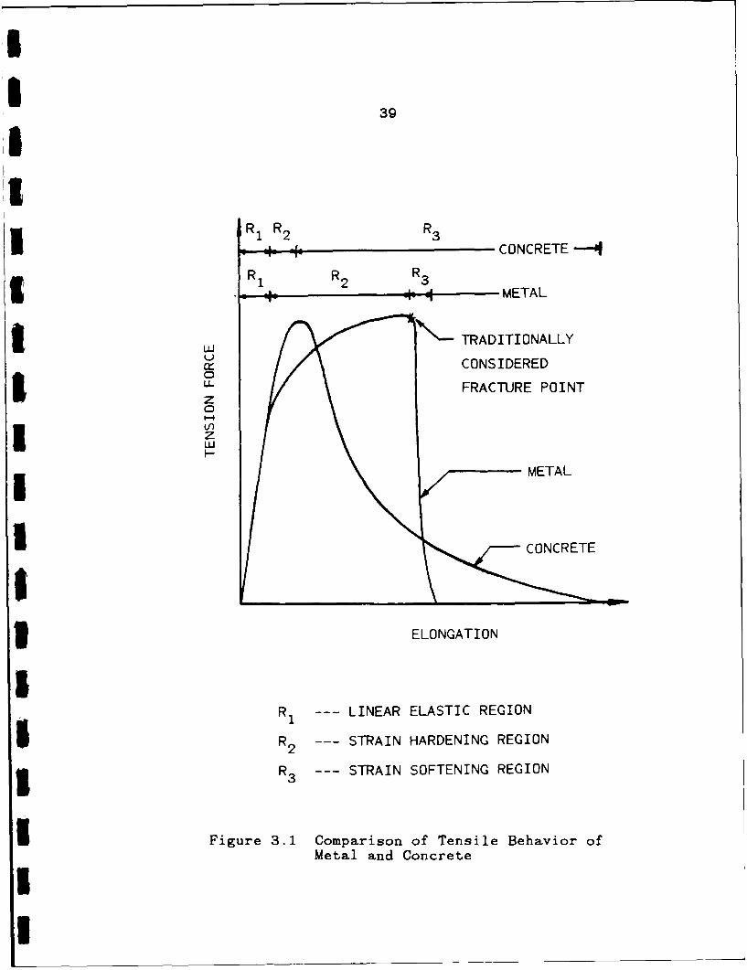
39
R1 R2 R3
* CONCRETE'
R1 R2 R3-£ L -J METAL
~CONSIDEREDI ul
U.FRACTURE POINTU
I CONCRETELNow
I3 ELONGATION
R 1 --- LINEAR ELASTIC REGION
I 2 --- STRAIN HARDENING REGION
I R3 --- STRAIN SOFTENING REGION
Figure 3.1 Comparison of Tensile Behavior ofMetal and Concrete
40
undergo a process in which the stress carrying ability
decreases from certain level to zero. Even in the fracture
mechanics books, the post-fracture material behavior is not
carefully considered. Generally, for any kind of material,
the tension curve can be divided into three regions, as
schematically illustrated in Figure 3.1, linear elastic
region, strain hardening region, and strain softening
region.
For homogeneous materials, such as metals, the strain
softening region is so small compared to the strain
hardening region, that the traditional fracture mechanics
does not need to study the tensile behavior in that region.
However, for nonhoxogenious materials, such as concrete,
the strain softening region is much larger than the strain
hardening region. This large size of strain softening
region is due to microcrack coalescing and aggregate
bridging in the materials.
3.1.2 Definition of fracture Process Zone
As a matter of fact, fracture is not a state but a
process which occurs between two different states. One
state is associated with perfect connection and the other
associated with completely separation of the material.
Thus, there must be an infinite number of intermediate
states associated with the partial connection. The
41
material which is undergoing this process constitutes the
fracture process zone.
In this dissertation, the fracture process zone is
defined as the region in which the tensile stress in the
material is decreasing from its maximum value to zero when
displacement controlled loads are applied.
On the other hand, fracture process zone can be
defined as the region of discontinuous microcracking ahead
of the continuous crack or as the partially damaged area
with some remaining stress transfer ability. Since in this
study, with only the mathematical models on macro-level is
concerned, the physical phenomena on either micro-level or
meso-level will not be studied.
3.1.3 The Role of Fracture Process Zone in Fracture
The material within the fracture process zone provides
a monotonically decreasing resistance to fracture with
fracture in progress. It is an energy absorber which makes
the material tougher or less brittle. The energy
dissipated to overcome the resistance is called work of
fracture, or custormarily the fracture energy. Although
for some material, such as glass, the fracture energy is
mainly the surface energy, for most other materials the
surface energy is much smaller than the energy which is
absorbed in the fracture process zone. For instance, the
42
surface energy is negligible compared to the energy
required for plastic deformation in metals or the energy
required to create microcracking and to overcome aggregate
bridging in cementitious materials.
3.2 Fracture Process Zone in Concrete
3.2.1 Observed Fracture Process Zone in Concrete
Fracture process zone in concrete was first measured
by Heilmann et al [107], using strain gages. A strain
value which is much larger than the maximum tensile strain
of the material was measured in a small region of a direct
tension specimens. As the strains in other regions
decrease beyond the peak load, the strains in this small
region still increase. The strain softening behavior,
i.e. the smaller the load the larger the strain was clearly
observed in that small region. Despite of the fact that
the strain gages gave only the average strain over its gage
length, this observation still proved the existance of
fracture process zone.
The fracture process zone were also revealed by many
test method. Using Scanning Electron Microscopy technique,
Dimond and Bentur [108] found that a system of very fine
multiple cracks appear in the vicinity of the crack. They
reported: "While the subdivision and branching seen to
43
occur near the tip zone in the concretes examined, is in
some respects reminiscent of what is expected in a 'process
zone', there is no physical distinction corresponding to
separate lengths of 'straight, open crack' behind a crack
tip and 'process zone microcracking' ahead of a crack tip."
Also using in-situ SEM observations, Tait and Garret [109]
did find a process zone of microcracking in the vicinity of
the crack tip of mortar or cement paste specimen.
3.2.2 Features of Fracture Process Zone in Concrete
Concrete is a heterogeneous material and its fracture
mechanism is much more complicated than that of homogeneous
materials. Despite its microscopic mechanism, the whole
fracture process can be divided into three subprocesses:
microcracking process, transition process, and aggregate
bridging process, as shown in Figure 3.2.
When a crack is extending in a concrete member, a
portion of the process zone adjacent to the microcrack tip
is in the microcracking process, while another portion of
the process zone closest to the crack mouth is in an
aggregate bridging process. The former is referred to the
microcracking zone, the latter the aggregate bridging zone,
and the middle portion the transition zone. As shown in
Figure 3.2, the transition zone can be recognized by a
relatively sharp drop of stress along the crack even though
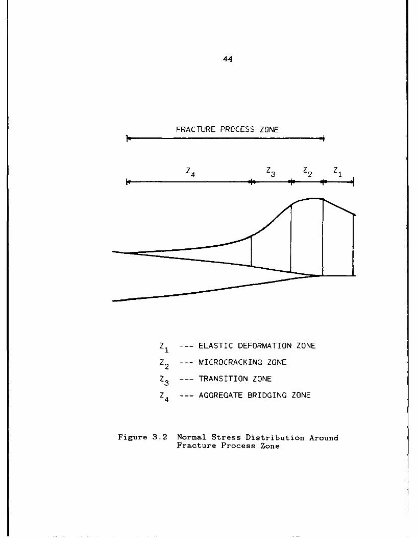
44
FRACTURE PROCESS ZONE
Z4 Z3 Z2 ZI
4.w -r - -
Z 1 - ELASTIC DEFORMATION ZONE
2 - MICROCRACKING ZONE
Z3 TRANSITION ZONE
Z4 - AGGREGATE BRIDGING ZONE
Figure 3.2 Normal Stress Distribution AroundFracture Process Zone
45
the boundaries are not well defined'
Another important feature of the fracture process zone
for concrete is the large size of that zone which brought
about new research topics to traditional fracture
mechanics. It is easy to see from Figure 3.1, that
concrete has a much different tension curve than metals.
Its strain hardening zone is very small but its strain
softening zone is very large. For metals, only the strain
hardening zone is of major concern in fracture mechanics
because it is much larger than the softening part.
Logically, for concrete the strain softening zone ought to
be of major concern.
3.2.3 Significance of Fracture Process Zone in Concrete
For those materials having small fracture process zone
(relative to the specimen size), the fracture resistance
stress is highly concentrated in that small region so that
it can be treated as a concentrate force. In this
situation, a single parameter, such as Kic., Gic, and JIc'
can be used to represent the magnitude of the fracture
resistance of the material.
In contrast, concrete and also other cementitious
materials usually have large fracture process zone (of the
same order of the specimen size), the fracture resistance
stress is distributed along the process zone and can no

46
longer be treated as a concentrate force. Obviously, a
single parameter model is not applicable. Moreover, the
distribution of the crack opening resistance stress is
specimen geometry and loading configuration dependent
rather than a material property.
An appropriate representation of the fracture
resistance of this kind of materials and the theory which
is able to predict both magnitude and distribution of
resistance stress along the fracture process zone in any
circumstances must be developed. This is the aim of this
study.
3.3 Method of Approach
3.3.1 Scope of Research
The structure of concrete has been subdivided into
three different levels [110]: micro, meso and macro. The
models on the different levels are interrelated in a
systematic way, or more precisely, models on a given level
are based on the results of the previous level.
At the micro-level, the structure of hardened cement
paste is treated. At the meso-level, the main
characteristics are big pores, pre-existing cracks and
inclusions. And at the macro-level, concrete is treated as
a continuum and homogeneous medium.
47
This study investigates and models the fracture of
concrete material only at the macro-level.
For simplicity, the strain hardening effect is not
considered since the strain hardening region is much
smaller than the strain softening region in concrete.
Finally, only Mode I fracture is studied in this
dissertation.
3.3.1 Mathematical Representation - Assumptions
Figure 3.3 shows the published direct tension test
results. These results suggest that a strain softening
representation should be included in the mathematical
model.
Three following basic assumptions are made to
construct a mathematical model for the tensile fracture
behavior of concrete:
1) The fracture process zone is represented by a crack
or a material discontinuity along a line with a closure
stress acting on the opposing crack surfaces.
2) The material outside the fracture process zone is
linearly elastic, homogeneous, and isotro - such that the
classical elasticity theory can be applied.
3) Inside the fracture process zone, the closure
stress is uniquely related to the crack opening
displacement by a non-increasing function of
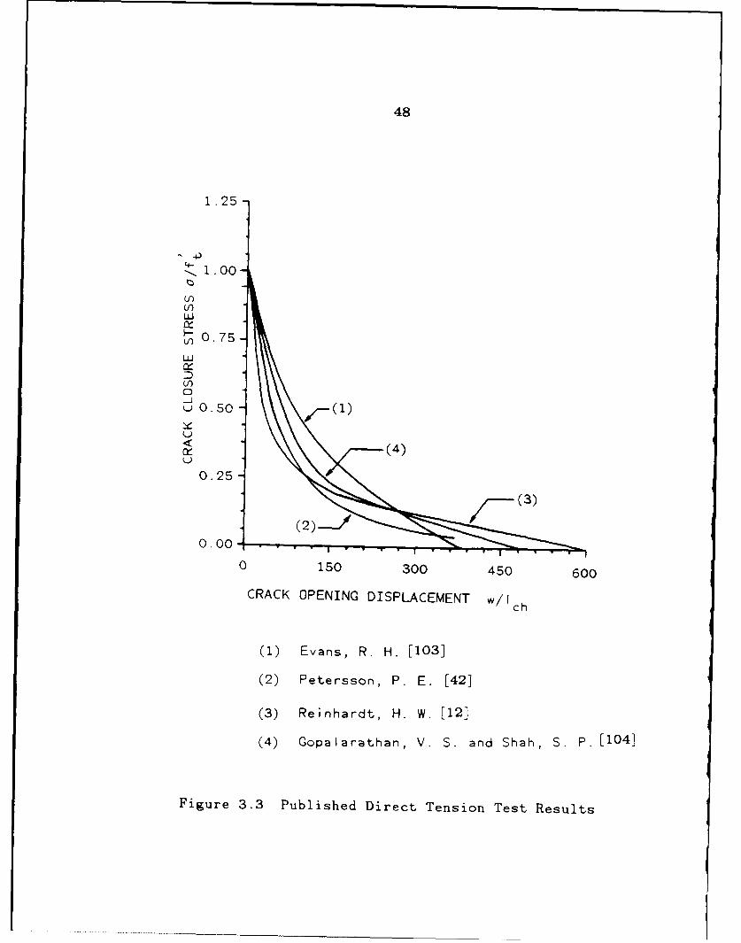
48
1 .25-
1.0
ul
LU
0O.50
(4)
0.25-
((3
0. 00
0 150 300 450 600
CRACK OPENING DISPLACEMENT w/I ch
(1) Evans, R. H. [1033
(2) Petersson, P. E. [423
(3) Reinhardt, H. W. [12]
(4) Gopalar-athan, V. S. and Shah, S. p. [104]
Figure 3.3 Published Direct Tension Test Results
49
0 = f (w) (3-1)
in which, a is the closure stress and w is the crack
opening displacement at the same position.
These basic assumptions will be justified by a series
of experimental and numerical investigations in the
subsequent chapters.
3.3.3 Hybrid Experimental - Numerical Approach
Following the hybrid experimental - numerical
technique by Kobayashi F111,112], this research consists of
two components. First, the laboratory tests are conducted
on concrete CLWL-DCB and three point bend specimens in
order to physically observe and measure the fracture
process zone and the deformation of the specimens. Second,
the test data are used as input to the finite element
analysis for determining the fracture parameters involved
in the fracture process zone model. The experimental
method used in this study is moire interferometry. The
numerical method is finite element analysis.
This investigation uses a two phase analyses [111],
the generation phase and the application phase. In the
generation phase, test data are used, through finite
element analysis, to generate the fracture parameter,
which, in this case, is the crack closure stress versus
50
crack opening displacement relation. In the application
phase, the fracture parameter is used as input to the
finite element analysis to predict the test results, which
is the crack propagation, COD, and all other specimen
behaviors.
CHAPTER FOUR
EXPERIMENTAL APPROACH
Experimental observation and measurements are
essential sources of information for a correct development
of the mathematical models of real materials. In this
chapter, a series of fracture tests of concrete specimens
are reported and a moire interferometry technique applied
to concrete fracture process zone measurement is presented.
4.1 Test Program
4.1.1 Objectives of the Experiments
In general, the objectives of the tests are to
physically observe the fracture process zone, to measure
its size and the crack opening displacement along its
extent, as well as the specimen response to the external
load. A replica film technique was used for detecting the
microcracking zone on the concrete specimen surface.
However, the use of the replica film technique can only
provide the information of crack length, and not the crack
opening displacement. Two clip-on gages (clip shape
extensometer) were used to measure the crack openings at
two locations, one was near the prenotch mouth, the other
was close to the prenotch tip. The former measured the
52
crack mouth opening displacement called 2V1 , the latter
measured the crack tip opening displacement called 2V2 .
Both crack opening displacement measurements are on the
prenotch. It is not possible to mount any mechanical or
electrical displacement transducer into the fracture
process zone region since the crack extension path is
unknown, and it is never straight. Apparently, the
information obtained in this stage did not include the
width of the fracture process zone nor the crack opening
along the process zone. The resultant theoretical model
thus was only relaying integrated and smeared information
of the process zone.
An advanced test method must be developed for
furthering the physical knowledge and also for improving
the theoretical model. The best candidate chosen is the
moire interferometry method since it provides a
full - field information. Moire interferometry is a new
displacement measuring technique which combines moire
effect with holographic interferometry. To develop a
application procedure for fracture of concrete research
will solve the above problems.
4.1.2 Test Groups and Test Variables
Five groups of specimens were tested using moire
interferometry. Three of them are CLWL-DCB specimens with
53
different sizes and different materials. The other two
groups are three point bend specimens of different sizes
and materials. The specimen dimensions are shown in
Figures 4.1 and 4.2.
The first group of investigation used small scale
three point bend specimens, as shown in Figure 4.1 (a),
because this is an exploratory and equipment limited
investigation.
In the second group an attempt was made to apply moire
interferometry method to the previously used CLWL-DCB
specimens '9], as shown in Figure 4.1 (b).
The third group had the same purpose as the second
group but used different material to check the aggregate
size dependency of the developed model. Specimens of the
same size and geometry as the third group were used.
The fourth group was used to generate fully developed
fracture process zone in the smaller CLWL-DCB specimens,
shown in Figure 4.2 (a). Fully developed fracture process
zone could not be obtained in 102 mm x 102 mm
(4 in. x 4 in.) area of these specimens.
The fifth group specimens were similar in size, and
the same material as the fourth group, but different
geometry, as shown in Figure 4.2 (b), to check the geometry
effect on the fracture process zone model.
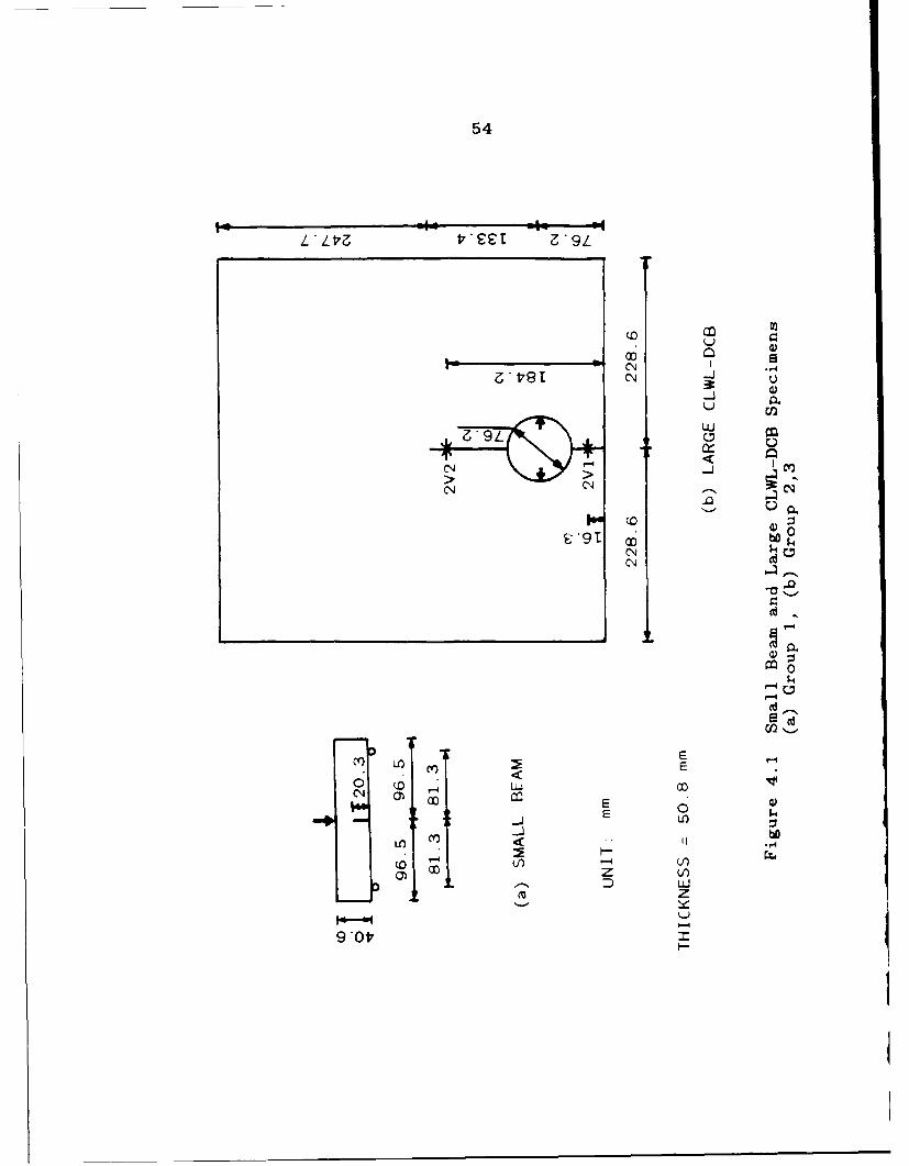
54
zsl ~9L
C.14
7, LU
(00
co0
'-4
-4u
0 ( 0E
E a,E-IO
(0 c.) ~.1bO(0 m (A4-
0V) Z Oa) U.)zL
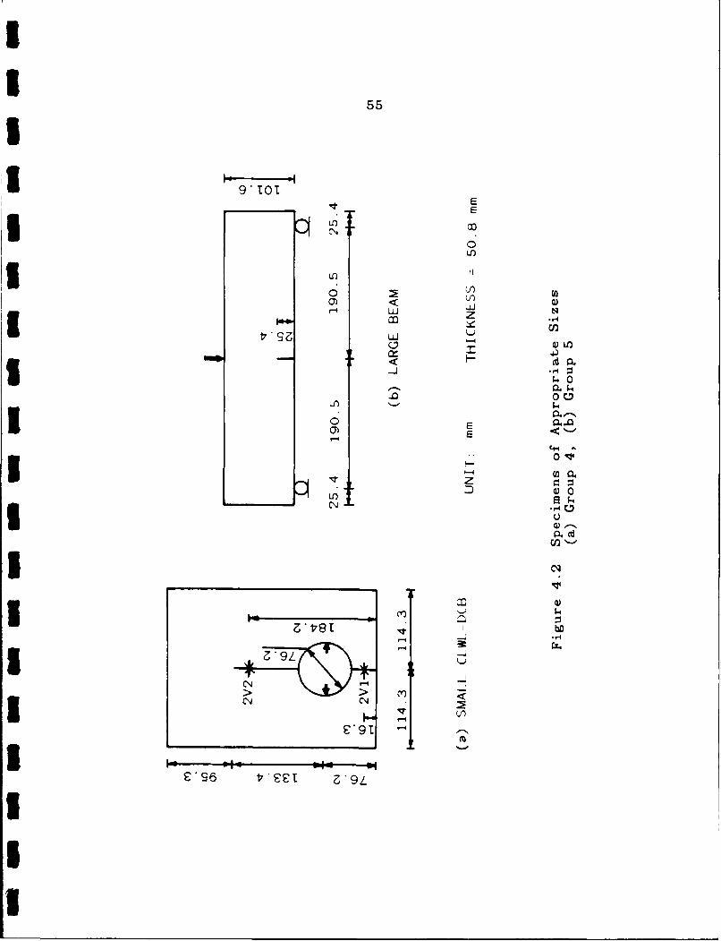
55
LtLO
IO I I
'-4 LUjI z-j-
-o -40
I 0 E'4-4I0
zI n tiIP C1
u)i.
I 9I >
£96 ~*~m
56
4.1.3 Loading and Data Recording Devices
Three different loading devices were used in this
investigation. A small screw drive loading fixture was
used for the first group. This fixture is made of C-chanel
steel. It is much more rigid than the small concrete three
point bend specimens so that a displacement controlled
loading condition was achieved. Starting from the second
group, larger specimens were tested. To accomodate large
specimens, a testing machine was needed. Only a simple
shop press was available when Groups 2 - 4 tests were
conducted. Fortunately, these CLWL-DCB specimens were
inherently rigid, and thus stable crack growth was obtained
with this simple machine in Groups 2 - 4. The previously
developed wedge load assembly and the adjustable specimen
holder, shown in Figure 4.3, were mounted on this shop
press. And the wedge load was applied manually. The shop
press was not suitable for these three point bend specimens
of fifth group because these specimens were less rigid than
double cantilever beam specimens. The third machine is a
screw-drive universal testing machine which induced stable
crack growth in these three point bend specimens.
In the CLWL-DCB specimen testing, an HP computer was
used to record the wedge load and the crack opening
displacements 2V 1 and 2V2 . For these three point bend
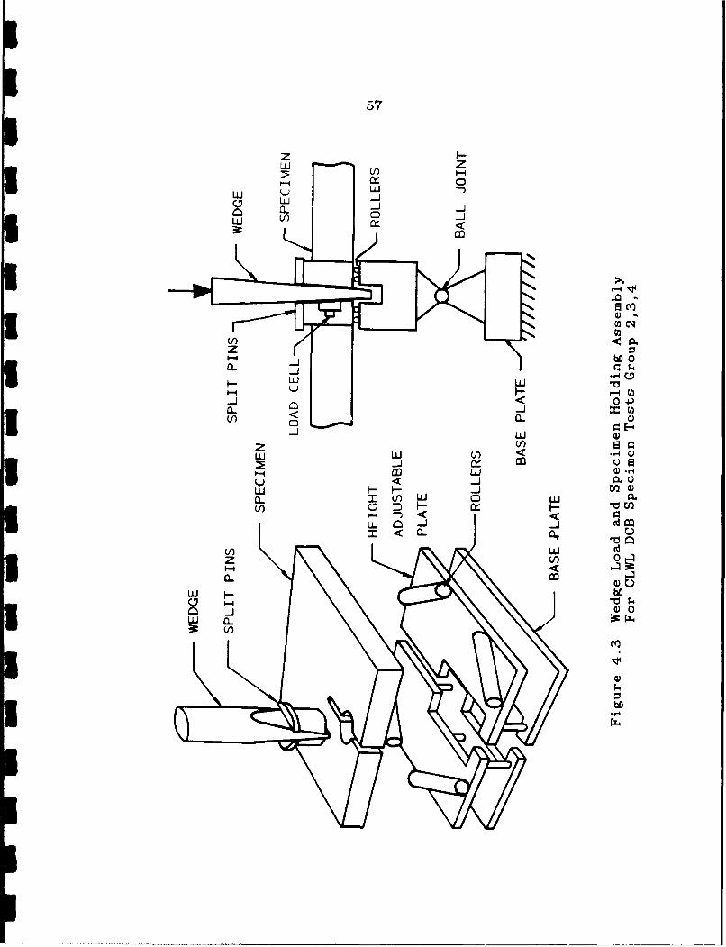
57
zHLU rz
UI-I
uj -,CL -J
u-J
0o
z V
LU *1- Q
0.
(I) 0 vE
(n LUz Ln 0.
a. co L
0~ 0-
bO.H-
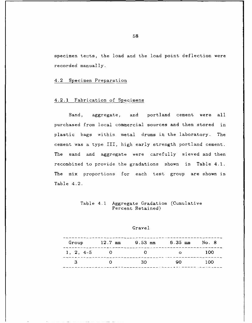
58
specimen tects, the load and the load point deflection were
recorded manually.
4.2 Specimen Preparation
4.2.1 Fabrication of Specimens
Sand, aggregate, and portland cement were all
purchased from local commercial sources and then stored in
plastic bags within metal drums in the laboratory. The
cement was a type III, high early strength portland cement.
The sand and aggregate were carefully sieved and then
recombined to provide the gradations shown in Table 4.1.
The mix proportions for each test group are shown in
Table 4.2.
Table 4.1 Aggregate Gradation (CumulativePercent Retained)
Gravel
Group 12.7 mm 9.53 mm 6.35 mm No. 8
1, 2, 4-5 0 0 o 100
3 0 30 90 100
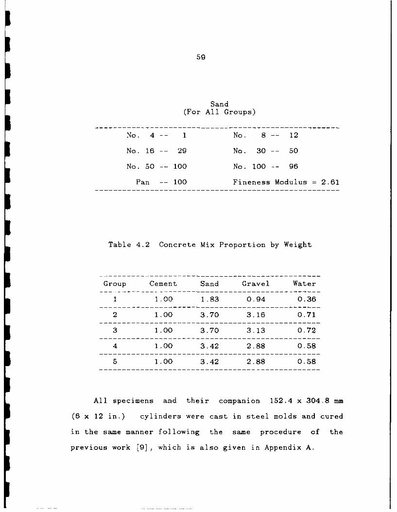
59
Sand(For All Groups)
No. 4-- 1 No. 8-- 12
No. 16 29 No. 30 -- 50
No. 50 -- 100 No. 100 -- 96
Pan -- 100 Fineness Modulus = 2.61
Table 4.2 Concrete Mix Proportion by Weight
Group Cement Sand Gravel Water
1 1.00 1.83 0.94 0.362 1.00 3.70 3.16 0.71
3 1.00 3.70 3.13 0.72
4 1.00 3.42 2.88 0.58
5 1.00 3.42 2.88 0.58
All specimens and their companion 152.4 x 304.8 mm
(6 x 12 in.) cylinders were cast in steel molds and cured
in the same manner following the same procedure of the
previous work [9], which is also given in Appendix A.
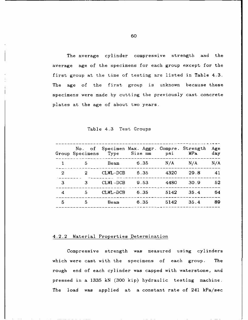
60
The average cylinder compressive strength and the
average age of the specimens for each group except for the
first group at the time of testing are listed in Table 4.3.
The age of the first group is unknown because these
specimens were made by cutting the previously cast concrete
plates at the age of about two years.
Table 4.3 Test Groups
No. of Specimen Max. Aggr. Compre. Strength Age
Group Specimens Type Size mm psi MPa day
1 5 Beam 6.35 N/A N/A N/A
2 2 CLWL-DCB 6.35 4320 29.8 41
3 3 CLWI-DCB 9.53 4480 30.9 52
4 5 CLWL-DCB 6.35 5142 35.4 64
5 5 Beam 6.35 5142 35.4 89
4.2.2 Material Properties Determination
Compressive strength was measured using cylinders
which were cast with the specimens of each group. The
rough end of each cylinder was capped with waterstone, and
pressed in a 1335 kN (300 kip) hydraulic testing machine.
The load was applied at a constant rate of 241 kPa/sec
61
(35 psi/sec). The average of measured value from five
cylinders of each cast batch of concrete was taken as the
material strength. The modulus of elasticity, E, and the
tensile strength ft was measured using
50.8 x 50.8 x 203.2 mm (2 x 2 x 8 in.) rectangular
specimens. These specimens were cut from broken CLWL-DCB
and three point bend specimens by a water cooled saw
machine after these specimens had been tested to failure.
The ends of the specimens then were glued with concrete
epoxy to steel blocks which in turn were connected to screw
bars. The other two sawed surfaces of the specimens were
sanded and cleaned and concrete strain gages of 50.8 mm
(2 in.) gage length were applied. After the epoxy was
cured, the specimens were mounted on a testing machine by
connecting universal joints to the screw bars. The loading
speeds were controlled at the same rate as that in the
CLWL-DCB or the beam tests. The load was applied three
times to approximately 30 % of the maximum load and the
average slope was used to evaluate tangential stiffness of
the specimen. The modulus of elasticity and tensile
strength were then calculated from the average of the
recorded data of two identical specimens for each batch.
These results are listed in Table 4.4.
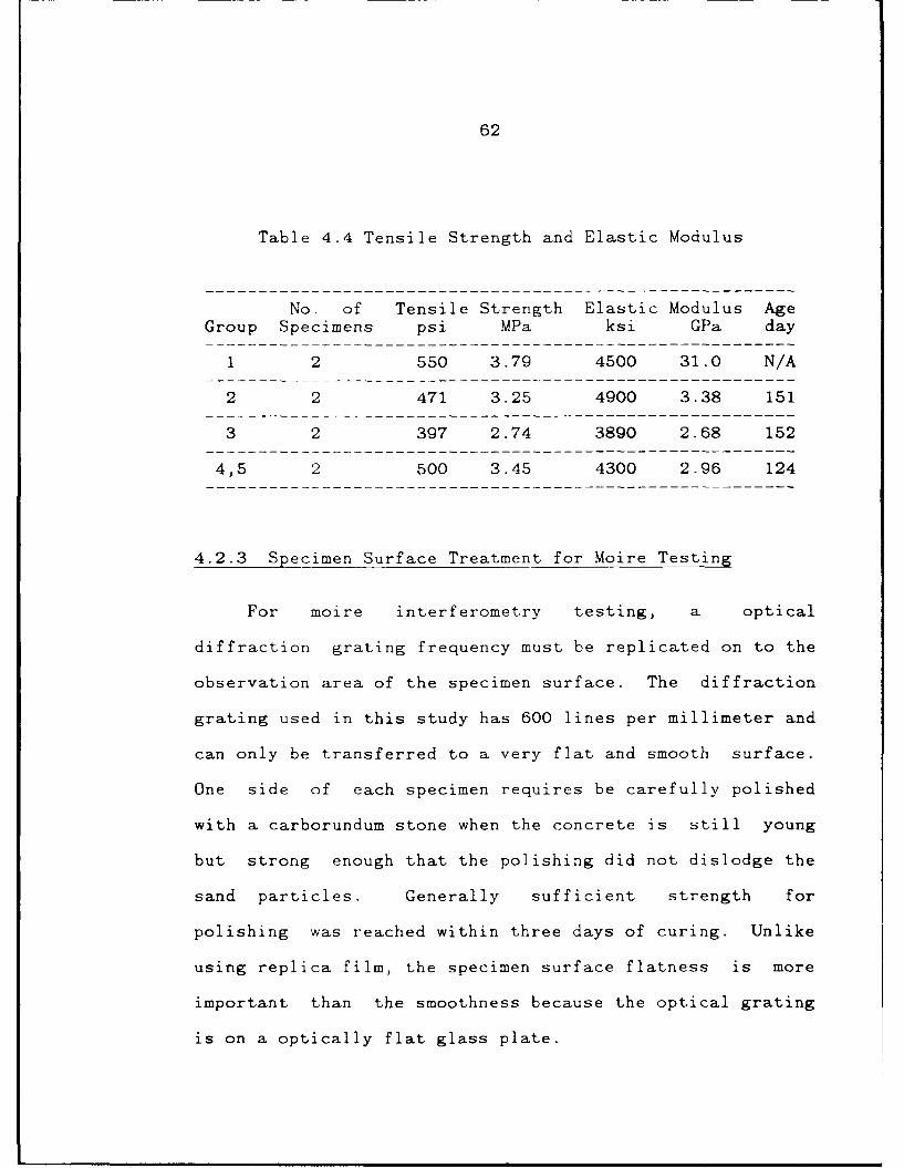
62
Table 4.4 Tensile Strength and Elastic Modulus
No. of Tensile Strength Elastic Modulus Age
Group Specimens psi MPa ksi GPa day
1 2 550 3.79 4500 31.0 N/A
2 2 471 3.25 4900 3.38 151
3 2 397 2.74 3890 2.68 152
4,5 2 500 3.45 4300 2.96 124
4.2.3 Specimen Surface Treatment for Moire Testing
For moire interferometry testing, a optical
diffraction grating frequency must be replicated on to the
observation area of the specimen surface. The diffraction
grating used in this study has 600 lines per millimeter and
can only be transferred to a very flat and smooth surface.
One side of each specimen requires be carefully polished
with a carborundum stone when the concrete is still young
but strong enough that the polishing did not dislodge the
sand particles. Generally sufficient strength for
polishing was reached within three days of curing. Unlike
using replica film, the specimen surface flatness is more
important than the smoothness because the optical grating
is on a optically flat glass plate.
63
4.3 Moire Interferometry Test Method
4.3.1 Introduction to Moire Interferometry Method
The fracture process zone in concrete is difficult to
determine experimentally, since the resulting deformation
is strongly localized and can not be measured adequately by
strain gages which provide only the average strain values
over the gage length. The sensitivity of the conventional
moire technique, on the other hand, is not adequate for
measuring the small tensile deformation in concrete prior
to its failure. The solution is to use moire
interferometry.
Moire interferometry is a full-field method of
measuring deformations of the surface of the specimen. The
result of a moire experiment is a fringe pattern, which is
a contour map of in-plane displacements in the direction
perpendicular to the lines of the diffraction grating
replicated on the specimen surface.
There are various methods for moire interferometry.
As mentioned in Chapter 2, the method Cedolin et al. [77]
used can only photograph images by collecting the scattered
light coming from the specimen grating so that the
resultant fringe patterns were not distinct. In order to
overcome this difficulty, a different method which was
64
originally proposed by Post [113] was used in this study..
Post's moire interferometry is based on the
interference of two symmetrically diffracted beams of
light. These beams are the first diffraction orders of two
mutually coherent, collimated beams of light that are used
to illuminate a specimen grating. Their interference
creates a fringe pattern. Figure 4.4 shows the basic
configuration of an optical system in which monochromatic
laser light is used. The mutual coherence of beams A and B
is achieved by a beamsplitter, or a plane mirror placed
near the specimen grating.
Two basic equations in optics are involved: first is
the interference of two intersecting beams, and second is
the diffraction of a beam on an optical grating. These
equations are:
f = (2/X) sino (4-1)
and
sin 8 = XFm sin7, (4-2)m
respectively, where:
f : frequency of the interference fringes
X : wavelength of the light
0 :half mutual angle of the two beams
F : frequency of the optical grating
m : order of diffraction
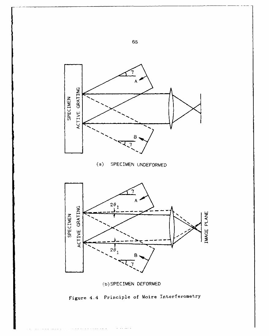
A
z
LU WU
a-S
B
(a) SPECIMEN UNDEFORMED
A
-% z
- L
LU LU 5.. -- - C
20BB
(b) SPECIMEN DEFORMED
Figure 4.4 Principle of Moire Interferometry
66
0 angle of the diffraction beam of order m.
y : angle of incident beam to the grating
as shown in Figure 4.4.
The specimen gratings used in this study were made by
holographically recording interference pattern of two
monochronic coherent laser beams. The half mutual angle
0 was determined by Equation (4-1) for the required
frequency, then, transferred to specimen surfaces so that
the deformation of the specimen was identical to the
deformation of the grating. Whenever the grating deformed,
the frequency of the grating changed.
As shown in Figure 4.4, the incident angles for beam A
and beam B are chosen in such a way that the plus first
order diffraction of one beam and minus first order
diffraction of the other beam are in the specimen grating
normal direction. These incident angles can be determined
by Equation (4-2) as
7 = T arcsin(fsX), when m = ± 1 (4-3)
or
f = (1/X)sin7, when m = ± 1 (4-4)
where, f represents the frequency of the specimen grating.s
These two diffraction beams also create a interference
fringe pattern on the specimen grating plane as well as in
the surrounding space. This is called "virtual grating"
67
because it is analogous to the reference grating in
geometrical moire and it is not real. Comparing (4-4) and
(4-1), it is easy to see that the interference fringe
pattern produced by these two diffraction beams has twice
frequence of the specimen grating has. This is the
difference between moire interferometry and geometrical
moire.
When the specimen grating deforms, as shown in
Figure 4.4, the two first order diffraction beams become
slightly offset to the normal of the specimen grating.
Using Equation (4-2), replacing F by fs/(l+E) and
eliminating y by (4-3), one obtains
sinQ1 =± f s E when m = 1. (4-5)
According to Equation (4-1), the frequency of the
interference fringes of these two diffraction beams is
fE = 2f E. (4-6)
Since 2f s equals the virtual grating frequency fv, the
resultant fringe gradient is proportional to the virtual
grating frequency and strain.
After integration, Equation (4-6) becomes
U = N / fv (4-7)
where, U is the displacement component in the direction
68
perpendicular to the lines of specimen grating. We might
note that this governing equation is common for geometrical
moire and moire interferometry, though the two differ in
the optical principles from which they were generated.
4.3.2 Moire interferometry with real reference grating
Moire interferometry measures small displacement by
comparing the phases of light waves. Any distance change
of a fraction of the light wave length in the optical path
before the interference pattern is formed can blur the
whole fringe pattern. Usually, all the optical devices,
the test specimen and the loading fixture must be fixed on
an isolation bench to prevent them from any vibration.
Such an arrangement requires that the test be conducted in
special equipped laboratory and the specimen as well as the
loading fixture must be small.
fraditionally, moire interferometry test is only
conducted on small specimens made of materials of small
grain size, such as metals or polymers. For concrete,
however, large size specimens must be used because of the
large aggregate size and big strong loading fixtures must
be used for big specimens to which the displacement
controlled load must be applied. The loading fixtures for
concrete testing usually are standard universal testing
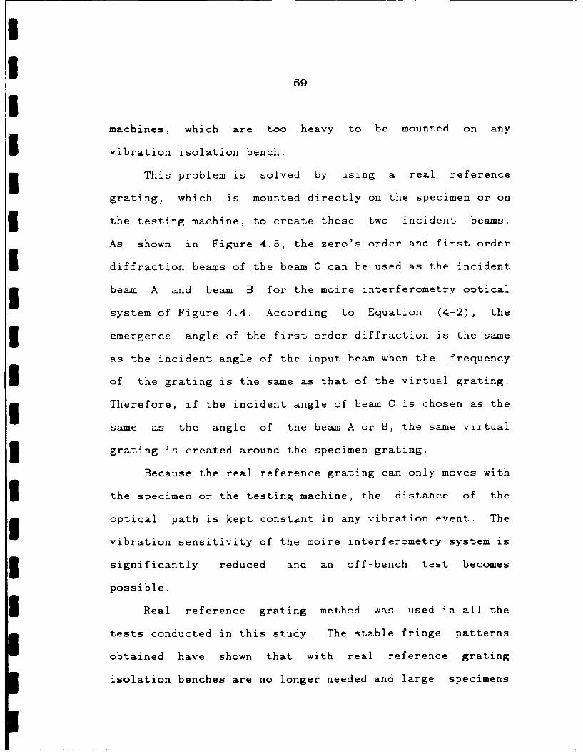
69
machines, which are too heavy to be mounted on any
I vibration isolation bench.
This problem is solved by using a real reference
grating, which is mounted directly on the specimen or on
the testing machine, to create these two incident beams.
As shown in Figure 4.5, the zero's order and first order
diffraction beams of the beam C can be used as the incident
beam A and beam B for the moire interferometry optical
system of Figure 4.4. According to Equation (4-2), the
emergence angle of the first order diffraction is the same
as the incident angle of the input beam when the frequency
of the grating is the same as that of the virtual grating.
Therefore, if the incident angle of beam C is chosen as the
same as the angle of the beam A or B, the same virtual
3 grating is created around the specimen grating.
Because the real reference grating can only moves with
I the specimen or the testing machine, the distance of the
optical path is kept constant in any vibration event. The
vibration sensitivity of the moire interferometry system is
significantly reduced and an off-bench test becomes
possible.
Real reference grating method was used in all the
tests conducted in this study. The stable fringe patterns
obtained have shown that with real reference grating
isolation benches are no longer needed and large specimens
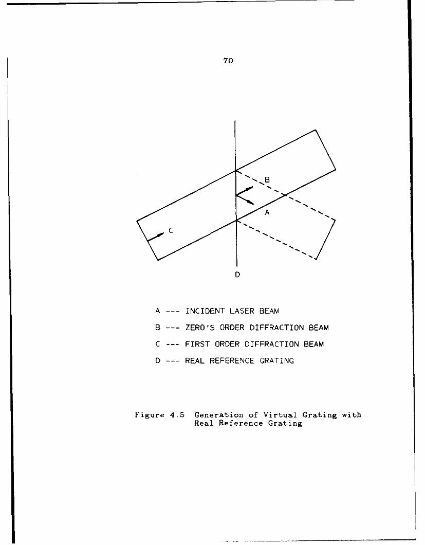
70
N% A
D
A -- INCIDENT LASER BEAM
B --- ZERO'S ORDER DIFFRACTION BEAM
C -- FIRST ORDER DIFFRACTION BEAM
D -- REAL REFERENCE GRATING
Figure 4.5 Generation of Virtual Grating withReal Reference Grating
71
can be tested by moire interferometry technique even
outside the optical laboratory.
4.3.3 Moire Interferometry With White Light
Due to the high cost of laser, monochronical light
source is not always available. In the first test group of
this study, a white light moire set-up constructed by Kang
[114] was used. The principle of white light moire is the
same as the laser moire with real reference grating except
that another optical grating called compensator is added to
the system to direct the incident beams of different
wavelength in correct angles, as shown in Figure 4.6.
From diffraction Equation (4-2), when the incident
angle is zero, the emergence angle of the first order
diffraction 91 is
0 1 = - arcsin (Fc X) (4-8)
where, F is the frequency of the compensator. Comparingc
(4-8) and (4-3), it is obvious that correct incident angles
for all the wavelength can be achieved by letting F equalc
to fS) which is the frequence of the specimen grating.
Furthermore, since the resulting fringe pattern is
indepcndent of wavelength (4-7), the fringe pattern
produced by the light of each wavelength is identical and
superimposed on each other.
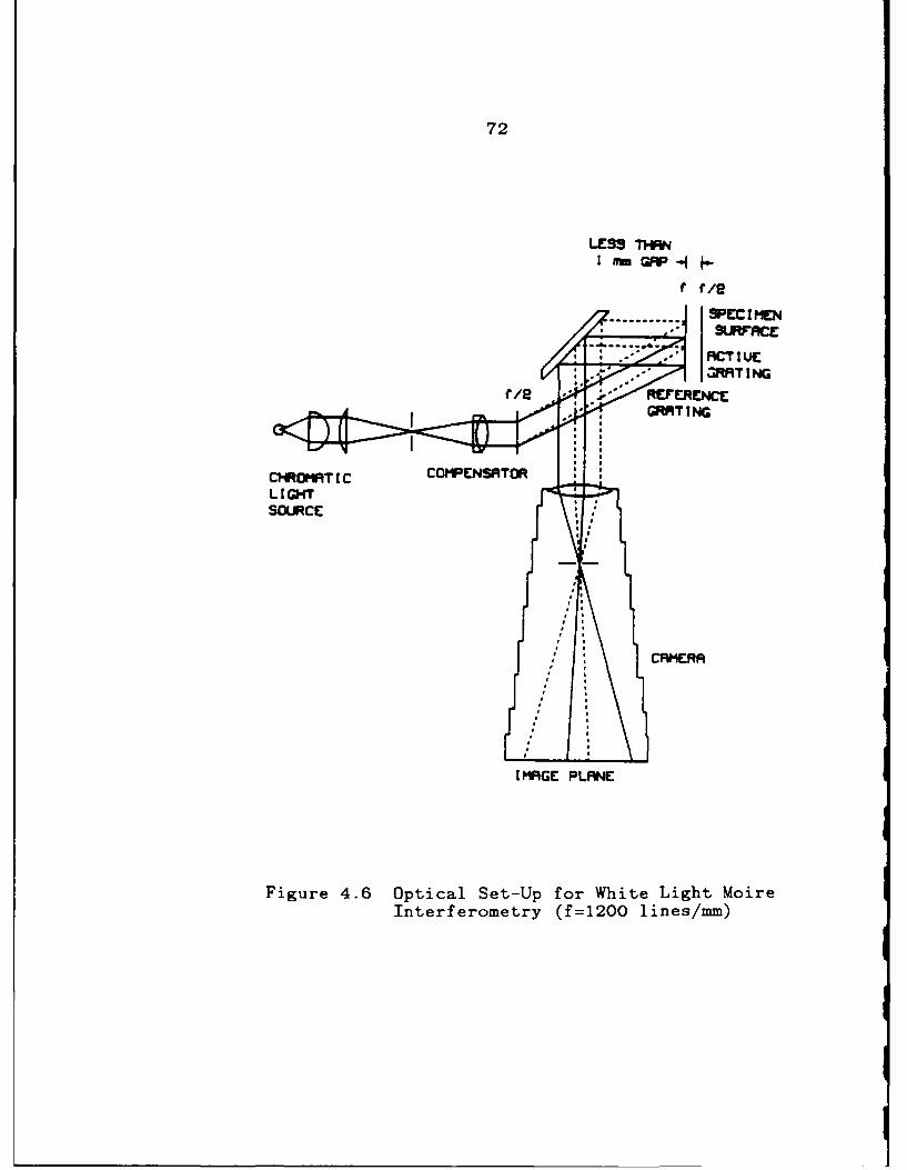
72
LESS THAN
f IV'S
GM~T I NG
CHROMATICG PLMENNEO
Figure 4.6 Optical Set-Up for White Light MoireInterferometry (f=1200 lines/mm)
73
4.4 Optical Instrumentation and Test Procedures
4.4.1 White Light Moire Set-Up
The optical arrangement of white light moire
interferometry is depicted in Figure 4.6. Here a mercury
light source is used in order to obtain higher light
intensity with smaller light source size. This is
important because the short coherence length problem of
white light source is compounded with a spatial coherence
problem. Each point in the finite light source generates
its own moire fringe pattern and all of these patterns will
be superimposed to form a blurred picture. Also the gap
between the real reference grating and the active grating
must be smaller than 1 mm to cope with the finite size of
the light source although it is smaller than 0.1 mm.
As shown schematically in Figure 4.6, the light from
the mercury lamp, which passes through a condenser
assembly, forms a collimated light beam. This lig't beam
then passes through the compensator grating with a wave
front of the diffraction order one. Although the zero's
order diffraction energy is wasted, about half of the total
energy is still taken with the first diffraction by having
chosen the first order preferred unsymmetrically ruled
grating as the compensator. The same consideration have
74
also been given to the design of the real reference grating
to make the intensities of the first order and zero's order Idiffraction beams approximately equal.
Because of the extremely short coherence length of the
white light, less than 1 mm, a very careful alignment must 3be done before moire fringe pattern can be obtained. Thus,
the light source, the compensator grating and the real Ireference grating all require provisions for minute
adjustments. Customer made stagings, using many
micrometers, have met this requirement. 3The final image of the moire fringe pattern is
recorded by a 35 mm camera which is operated either"I
manually or automatically. Black and white ASA 400 films
are used as recording medium and a zoom lens "- used to
obtain the desired image size on the film plane. 34.4.2 Laser Moire Set-u 3
The optical arrangement of the laser moire
interferometry tests are given in Figure 4.7. A 5 watt
water-cool argon laser was used as the light source. The 3real reference grating and specimen gratings were also made
with this laser on an isolation bench. 3The output laser light beam of intensity about 100 mw
is expanded after "cleaned" by a spatial filter and then Icollimated by a 152.4 mm (6 in.) diameter parabolic mirror I
I
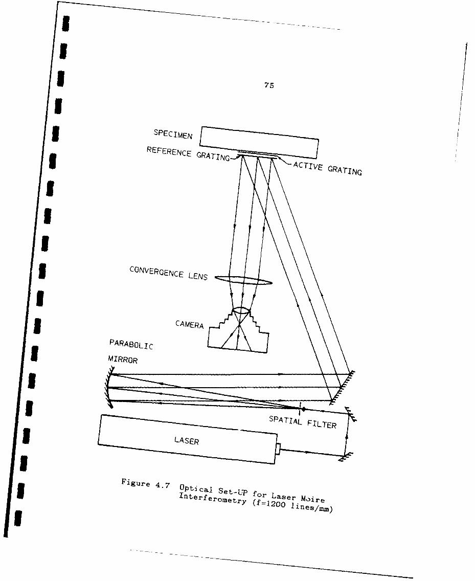
17
SPECIMEN/
REFERENCE GRATING ~ ~ACTIVE CRATING
CONVERGENCE LENS
I CAMERA
PARABOLI Cf MIRROR
IV
IFigure 4.7 lPtcalSetU.
for Laser MoireIer f10 ie/m
76
to provide a square field of 102 x 102 mm (4 x 4 in.).
This expanded laser beam was projected onto a flat mirror
mounted on the loading machine for double cantilever beam
test or mounted near the loading machine for three point
bend specimen test. These two machines were all located in
another room next to the laser lab.
Real reference grating technique was used in these
tests for vibration control. The frequency of the real
reference grating was 1200 line per millimeter. When the
laser beam was directed by that flat mirror onto the real
reference grating which sat right on the specimen upper
surface, the transmitted light through the real reference
grating and the first order diffraction light generated a
virtual grating field around the specimen grating. The
specimen grating had only one half density of lines, 600
line per millimeter, as virtual grating had.
All lenses and mirrors must be of high quality. The 3surface flatness or smoothness must be in the order of a
fraction of light wavelength to ensure a perfect wave front
before the laser reaches the specimen grating. For this 3kind of optical devices, if large sizes are required, they
are not easy to make and rarely commercially availlable. 3When the deformation event occurs, an interference
fringe pattern, which can clearly be seen by naked eyes,
appears on the specimen grating surface. This output light 3
U
77
image is first collected by a large diameter objective lens
with the help of a simple flat mirror. It, then, passes
3 through a image lens to form a real image for further
recording. Finally, this fringe image is recorded on a 35
1 millimeter film through an ordinary camera without camera
lens. The optical devices which record the formed fringe
3 pattern need not be of special high quality. And the
optical design of this recording system is based only on
elementary geometrical optics. Stagings and all other
adjustment devices were purchased except that for real
* reference grating was home-made.
3 Experience and error analysis [114] have shown that
for real reference grating, only in-plane rotation is
Ssensitive to adjustment. Thus, a very simple, economical
staging for the real reference grating was made. With a
I micrometer quality screw, 40 threads per inch, a fine and
3 smooth in-plane angle change was accomplished. This device
is shown in Figure 4.8.
3 4.4.3 Test Procedures
I The major steps in running a test are listed in the
3 following.
1) Transfer a grating to specimen. Due to the
3 porosity of the concrete, precoating is preferred for
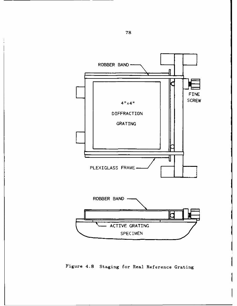
78
ROBBER BAND----\
FINE
4" x4" SCREW
DIFFRACTION
GRATINO
PLEXIGLASS FRAME---
ROBBER BAND - \
SPECIMEN
Figure 4.8 Staging for Real Reference Grating
79
reducing the absorption which may cause roughness of the
transferred result or even failure. Details of this
technique is given in Appendix B.
2) Mount the specimen to the testing machine. For
Wedge Loaded Double Cantilever Beam specimens, the
out-plane bending effect has to be checked and eliminated
before the actual test is started as described in ASTM
Standard 561 [115] and Reference [9]. For beam specimens,
small metal plates must be glued to the loading area of the
specimen to reduce stress concentration and the statically
determinate loading condition must be checked.
3) Align optical system. Using real reference grating
and laser, the optical system is very easy to align.
Actually, only the incident angle of the laser beam and the
in-plane rotation of the real reference grating need be
carefully aligned to obtain the minimum null pattern. If
white light is used as light source, the alignment is much
more difficult due to the short coherence length. In that
case, everything must be aligned in order to obtain a clear
fringe pattern. The camera must be focused with the help
of another scattered light source since parallel light of
the laser beam does not provide any target for focussing.
4) Apply displacement to the specimen. The
displacement controlled load must be applied slowly,
smoothly, and continuously. Any impact could alter the

80
result or even break the specimen.
5) Record moire fringe pattern, load and
displacements. The initial record should be taken before
load is applied and each picture should be taken at the
same moment as the load and displacements are recorded.
The use of a 35 mm camera is recommended because it is fast
and sequential pictures can be obtained if a motor drive is
used.
CHAPTER FIVE
NUMERICAL PROCEDURES
Research on numerical procedures involved in this
study is based on finite element analysis and is a
continuation of the finite element investigation on
fracture of concrete conducted at University of Washington.
The models developed in the previours study are refined and
new models as well as new numerical procedures are
developed. This chapter describes these developments
5.1 Finite Element Analysis
5.1.1 Special Features in Finite ELement Analysis
As defined in Chapter 3, the fracture process zone
model treats the material outside the fracture process zone
as linearly elastic and the material inside the fracture
process zone and only along the crack line as nonlinear
relaxed. Thus, any linearly elastic finite element code
can be used for this analysis provided that the boundary
condition along the fracture process zone is properly
treated. In some finite element programs, linear elastic
boundary condition, which prescribes springs to the
boundary nodes, is available. No iteration is needed in
this nonlinear analysis but the springs can not model
82
strain softening effect. The reason is that the springs
have larger deformation with greater force. This is just
opposite to the softening behavior. The essential point is
that a nonlinear problem can never be solved by a linear
routine no matter what kind of strategy is used.
Therefore, a linear finite element program with
nonlinear boundary conditions, in which iteration is
necessary for solving this nonlinear problem, must be
developed. According to the assumptions in Chapter 3, the
mode I fracture problem is defined as that illustrated in
Figure 5.1. There are two special features in this
problem. First, the boundary condition along the fracture
process zone is given indirectly by relating the normal
stress and displacement. Second, one of the external loads
can not be given if a maximum tensile stress criterion is
prescribed at the crack tip or vice versa.
Such defined problems can be solved in the following
steps:
1) Assume a crack closure stress versus crack opening
displacement relation, which is the constitutive equation.
2) Assume an initial stress distribution along the
boundary including the entire crack surface and an initial
unknown external load.
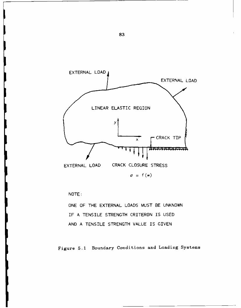
83
EXTERNAL LOAD
EXTERNAL LOAD
LINEAR ELASTIC REGION
x FCRC TIP
EXTERNAL LOAD CRACK CLOSURE STRESS
a = f (w)
NOTE:
ONE OF THE EXTERNAL LOADS MUST BE UNKNOWN
IF A TENSILE STRENGTH CRITERON IS USED
AND A TENSILE STRENGTH VALUE IS GIVEN
Figure 5.1 Boundary Conditions and Loading Systems
84
3) Apply all the external loads including the initial
stress distribution and compute the tensile stress at the
crack tip element and the displacement field.
4) Correct the initial crack closure stress
distribution according to the constitutive equation in 1)
and using the computed displacement data in 3).
5) Correct the initial external load according to the
tensile strength of the material and the computed crack tip
tensile stress in 3).
6) Apply all the loads again, compute again, and
correct again.
7) Compare the corrections with the corrected values
of the unknown load and crack closure stress or crack
opening displacement to determine if they have already
converged into a acceptable limit.
8) Return to 4) if they have not converged,
otherwise, advance the crack tip one element size by
releasing the corresponding crack tip node.
9) Return to 2) and repeatedly follow 2) through 9)
until the running crack tip reaches the specimen boundary.
10) Compare computed results with test results to
make sure that the assumed constitutive equation in 1) is
correct, otherwise, go back to 1) to assume a modified
constitutive equation based on experiences.
85
This is the most normal solution method, but it is
only good for explaining the principle because there are
too many finite element computations involved which need
too much computing time. Therefore, a more efficient
solution method has been developed which takes the
advantage of the superposition principle.
5.1.2 Superposition Principle and Fundamental Solutions
Superposition principle holds for any linear system.
With the help of this principle, the solution of a linear
system can be obtained by linearly superimposing other
known solutions. For linear elasticity, the external loads
are linearly related to any displacement component and also
any stress component at any point inside the elastic
domain. Green functions of displacement and stress of unit
load at a certain point can be used as these known
solutions and easily be computed using finite element
method if the analytical solution can not be derived. The
advantage of this method is that once the Green functions,
which are called fundamental solutions in this
dissertation, are known, no additional finite element
computation is needed.
86
The fundamental solutions can be obtained simply by
using finite element analysis to solve for a prescribed
unit load at a certain point and compute the displacements
and stresses at other points of interest.
One thing should be pointed out is that Green function
for unit displacement does not exist because no
displacement can be applied to a point of a elastic body
exclusively without disturbing the displacement of the
adjacent area. It is easy to understand that if the
adjacent displacement field is changed the applied
displacement can not be considered as only applied to one
point. This concept is sometimes confused and it is
worthwhile to clarify.
5.1.3 Formulation Using Fundamental Solutions
The basic governing equations for the linear elastic
domain with nonlinear boundary conditions can be formulated
using fundamental solutions. Suppose the fundamental
solutions have already been computed, then, according to
the superposition principle, the following equations can be
established:
Nwk = P wkP + F wkF + Wjk RP k 1,...,N, (5-1)
j-ljkj
87
NUTP P + 0TF F = ft jE aTj Rj, (5-2)
or. = f(w ), j = 1, N, (5-3)J J ' '
R %-l/ + 2 a j+/6)ab, j 1,.. .,N, (5-4)
where, constants:
a : element size along fracture process zone;
b : thickness;
F : prescribed external load;
variables:
P : unknown external load;
R. : equivalent load at node j;J
w. : COD at node j;J
w. : COD at node k;3
or. : surface traction at the position of node j;3
and fundamental solutions:
wkp : COD at node k due to unit P load at its node;
wkF : COD at node k due to unit F load at its node;
Wkj : COD at node k due to unit R load at node j;
ap : stress at crack tip due to unit P load at its node;
a TF stress at crack tip due to unit F load at its node;
aTj : stress at crack tip due to unit R load at node j.
Equations (5-1) are the relations between the CODs and all
the loads, including the crack closure forces applied to
88
the elastic domain. Equation (5-2) is the tensile strength
criterion. Equations (5-3) are the constitutive relations
of COD and crack closure stress. Equations (5-4) are the
equivalence relations of nodal forces and the corresponding
tractions along the fracture process zone. There are N
equations in (5-1), (5-3) and (5-4), respectively, and one
equation in (5-2). The total number of equations is 3N+l.
Suppose the function y = f(x) in Equations (5-3) is
known, the unknown variables are w., a., R., j = 1, N
and P (note F is known applied load ). The total number of
unknowns is 3N+1, the same as the number of equations.
Thus, these equations are solvable. Since this is a set of
nonlinear equations, an iteration method must be applied.
For CLWL-DCB specimen, the crack mouth opening displacement
2V and the crack tip opening displacement 2V2 can be
computed as:
N2V 1 = P V + F V1F + 1Vlj RP (5-5)j-=
N2V2 = P V2P + F V2F +l 2j RjY (5-6)
j=1
where, fundamental solutions:
Vp : 2V1 due to unit P load at its node;
V 1F: 2V 1 due to unit F load at its node;
89
Vj : 2V 1 due to unit R. load at node j;V 2P: 2V2 due to unit P load at its node;
V2F: 2V2 due to unit F load at its node;
V2j: 2V 2 due to unit R load at node j.
For three point bend beam specimen, the load point
displacement D can be determined as:
ND = D P + D F + E D. R., (5-7)
P F j=l J
where, fundamental solutions:
Dp : D due to unit P load at its node;
DF: D due to unit F load at its node;
D. : D due to unit R. load at node j.J J
Equations (5-1) through (5-7) are basic equations of the
formulation.
5.2 Indirect Method
5.2.1 Three - Line Model
An indirect method of solving for fracture parameters
was developed. This method is based on a three line model
which relates crack closure stress to crack opening
displacement by three straight lines segmented by three
critical CODs, w1 , w2 ) and w3 ) as shown in Figure 5.2.
90
For small CODs, 0 < w < wI , the fracture process zone
consists of coalescing microcracks. That segment can
sustain a closure stress equal to the maximum crack opening
resistance defined here as the tensile strength, ft" For
intermediate range CODs, w1 < w < w2, the closure stress
drops sharply with increasing CODs to a closure stress that
is only a fraction of ft The strain-softening behavior
for that segment reflects the spreading of the
micro-cracks. Petersson [42] found that the closure stress
at the trailing end of that segment to be equal to
one-third of the maximum closure stress for his small sized
specimen. For the large specimens a similar value of 0.3
ft was found to be appropriate. For CODs ranging between
w 2 and w3 , the closure stress decreases slowly from 0.3 ft
to zero. The fracture process zone terminated at w3 and
the crack can no longer transmit tensile stresses.
The three-line model can also be described in
mathematical form as:
r fr, 0 < w < Wl,
= ft[.7(w - w2 )/(w 1 - w 2 ) + . 3 ] , w1 < w < w2 , (5-8)
' ft[ '3(w -w )/(w2- w3 )], w2 < w < w3 .
In addition, a = 0, when w > w3 . These three CODs must be
obtained through a trial and error procedure.
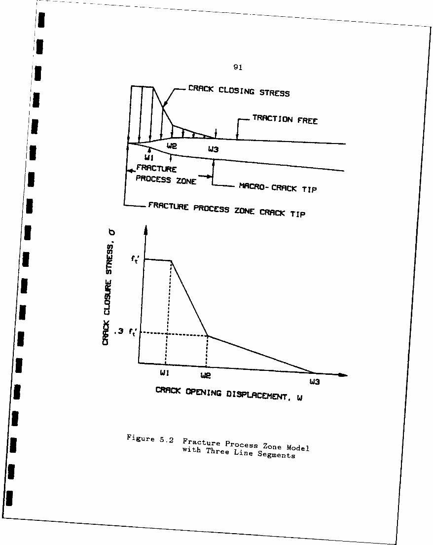
'3 91
CRACK CLOSING STRESS
II
PROCESS ZONE: I1ROp- CRA9CK TI P
I S
I iSII
3 w
CRACK OPENING D SPL.CEIIENT. W
Figure 5.2 Fracture Process Zone Modelwith Three Line Segment
sI
L_
92
5.2.2 Iterative Solution Scheme
To solve the basic equations given in 5.1.3 using the
indirect method and three-line model, a iterative schame
was established. Let ]i be representing ith iteration.
the iterative schame can be summarized as follows:
1. Estimate the initial CODs wk]O, k = 1,...,N.
Experience showed that those initial values could be given
zero values.
2. Compute the corresponding surface tractions Lk]O
based on a assumed closure stress versus crack opening
displacement relation, Equations (5-3).
3. Evaluate the equivalent nodal forces Rko, using
Equations (5-4).
4. During the i th iteration, compute unknown load P
by Equation (5-2).
5. Compute the resulting CODs for the load along the
fracture process zone by Equations (5-1).
6. Compute the corresponding surface traction Uk]i
based on the assumed a - w relation which is Equations
(5-3).
7. Evaluate the equivalent nodal forces Rk]i by
Equations (5-4).
93
8. Repeat steps 4 through 7 until convergence is
I reached as defined by:
W k]i - wk]i-1/wk]i < 0.01
9. Compute 2V 1 and 2V2 for CLWL-DCB specimens or
deflection at mid-span of three point bend specimens by
Equations (5-5) and (5-6) or (5-7), respectively.
Once the iterative procedure for the (N+l)th node is
completed, the microcrack tip is then advanced to the next
node and the iterative scheme is repeated until the
specimen boundary is reached.
5.2.3 Trial and Error Procedure
The computed results of load, 2V1 and 2V2 or
deflections of beam specimens are compared to test results.
If they do not agree with each other, changes must be made
in the assumed a - w relation. The whole steps given in
5.2.2. must then be repeated. Usually, such a trial and
error procedure is very tedious. This is the drawback of
the indirect method.
5.3 Direct Method To Determine o - w Relation
5.3.1 Motivations
The fracture process zone model characterized by
a a - w relation for concrete and similar materials has
94
been widely accepted. The question left now is how to
appropriately determine this relation. Although direct
tension test seems to be a solution, there are many
difficulties in conducting such tests. For example, an
extremly high stiffness is required for the testing machine
and possible eccentric loading due to material
non-homogeneities or axial misalignment are serious
drawbacks for a direct tension test.
In order to study specimen geometry effects, boundary
effects, and overall stress state effects on 0 - w
relation, specimens other than direct tension specimen must
be tested and results analyzed. An effective, convenient,
reasonable and reliable procedure to determine o - w
relation from test data is needed.
In the absence of direct tension data, measured GF
values have been used , together with measured tensile
strengths, to determine the constitutive equation. The
quantity GF, the area under the a - w curve can, however,
be used only for a model that is a straight line
approximation or is an assumed function for the crack
closure stress versus COD relationship. Since it has been
found that model predictions of specimen response are very
sensitive to the assumed function even for functions with
the same GF and tensile strength values, and accurate
measurement of GF is also difficult, this approach is
I95I
neither appropriate nor complete.
In order to determine accurately an appropriate
3 function the measured global responses of the specimen must
be used to check the assumed function by comparing them
3 with corresponding numerical predictions and then making
changes as needed in the form of the function. This is the
indirect method described in the former section or called
3 trial and error procedure. For three-line modell six
unknown parameters must be determined. If ten different
3 values are tried for each parameter, a million computations
must be executed for advancing the crack tip only one step.
Such procedures are not only very tedious and time
3 consuming but also suffer from uncertainty in the
solution's uniqueness as well as the lack of a benchmark
3 solution for computation.
When crack opening displacements along the fracture
I process zone have been measured by moire interferometry,
3 Those displacements can be taken as input displacement
boundary conditions for a finite element computation to
3 find crack closure stresses along that boundary. As soon
as crack closure stresses are determined, the relationship
I between the crack closure stress and crack opening
displacement, which has already been measured in the test,
is determined. However, that procedure has a potential
3 problem. The solution is very sensitive to errors in the
ver
96
input data resulting from boundary displacements which have
been erroneously recorded due to unavoidable experimental
errors.
Because of the relatively large variations in test
results for geomaterials, such as concrete, raw test data
should never be used directly. An optimization procedure
should be used in smoothly model the test data for
numerical analyses. Since the a - w model has been studied
for more than ten years, the general shape of a - w curve
is well known and an appropriate mathematical form can be
readily incorporated in the optimization procedure.
5.3.2 One - Curve Model
The U - w relationship for three-line model cannot be
expressed as a single function form and is not continuously
differentiable. In order to set up an optimization
procedure, the corners of the three line model must be
rounded and an appropriate function found to replace these
three lines. A smooth curve is also more logical for
macro-level modeling.
An appropriate function must satisfy the following
conditions:
1. Tt has to be a monotonically decreasing function.
This means that the first derivative must always be
negative except at its two boundaries.
I97
2. When w = 0, a = ft and da/dw = 0 , where ft is
* tensile strength of the material.
3. When w = 00 , 0 =. (This is only a approximate
modeling).
3 4. It must have the same general shape as the U - w
curve already established for concrete. The shape must
also be changeable by adjusting parameters.
5. The total number of the parameters must be as
small as possible but the shape and size of the curve must
also be sensitive to the changes in those parameters. In
other words, each parameter must have a distinct influence
on the shape or the size of the curve.
The function chosen is
S= (5-9)1 + 2(w/) p
in which a > 0 and 8 > 1. This function satisfiies all
five conditions. Conditions 1 - 3 can be easily checked by
taking the first order derivative. Conditions 4 and 5 can
be checked by using Figure 5.3. Obviously, ft and a are
scaling factors for the a and w coordinates, respectively,
and C controls the shape of the curve. It can be seen from
Figure 5.3 that smaller f values correspond to a smaller
microcracking zone and a larger aggregate bridging zone,
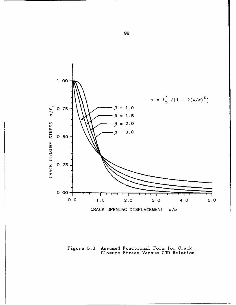
98
1 .00-
f ) f /[1 +(/)
40.75- p 1. 0
tz, 1.5
U-) p 2. 0UI)U-i
p=3. 0vI) 0.50-
LU
:DVI)
(-)
z0.25-
0.00-1 1 11 1 -- 1 v a,
0.0 1.0 2.0 3.0 4.0 5.0
CRACK OPENING DISPLACEMENT w/a
Figure 5.3 Assumed Functional Form for CrackClosure Stress Versus COD Relation
99
and vice versa. Also, the parameter, a, has a physical
meaning. When w = a, = 3 no matter what value P has.
One third f is the stress level at the division betweent
microcracking and aggregate bridging. Thus a is the crack
opening displacement at this division and is equal to w2 in
Three-Line model.
5.3.3 Optimization Procedure
Once the functional form is established, the
parameters in the function can be determined by fitting the
test data through an optimization procedure. For
simplicity, the nodal force versus traction relationships,
or Equations (5-4), were replaced by the expression.
Rj = ab a j, j = 1,...,N (5-10)
in this study. For the functional form of Equation (5-9),
Equations (5-3) become.
fa. = t, j = 1,.. .,N. (5-li)
S 1 + 2(wji/a) '
Substituting Equations (5-11) into Equations (5-10) and
substituting Equations (5-10) into Equations (5-1) and
(5-2), for F = 0, gives:
100
N w ft abw k = p w kp + E. k =1,. N, ( -2
j=l 1 + 2(w /a)
N a f abor P =f ft (5-13)TP P j=i 1 + 2(w /a)
Equations (5-12) and (5-13) constitute a set of N+1
equations. The unknowns in these equations are fracture
parameters ft' a and P. Since N is much larger than 2,
this is an overdeterministic set of equations. In the case
of CLWL-DCB specimens, two more equations can be added to
fit the measured 2V1 and 2V2 . Through a similar
derivation, these equations can be written as:
N V f ab2V1 = P +V 1 +t E (5-14)
j=l 1 + 2(w /a)
N Vjftb
2V = P V 2 2j ft ab (5-15)2 2P j=1 1 + 2(wj
For three point bend specimens, the load point deflection
can be fitted with:
N D. ft abD = Dp P + E t (5-16)
j=1 1 + 2(wj/a)
A set of Equations (5-12) , (5-13) , (5-14) , (5-15) are
101
used for the analysis of the CLWL-DCB specimen and another
set of Equations (5-12), (5-13), (5-16) are used for the
three point bend specimen. Each set of equations can be
written using the test data measured for certain crack
length. Multiple sets of such equations corresponding to
the different crack growth stages were solved simultanously
to obtain an unique set of fracture parameterss The
solution scheme included a Newton-Raphson routine and a
Householder transformation. Additional details are given
in Appendix C.
5.4 Discussion on Numerical Procedure
5.4.1 Prediction of Crack Propagation
As stated in Chapter 3, this hybrid analysis consists
of two phases, i.e. The generation phase and the
application phase. In the generation phase of analysis,
the constitutive law, which is a fracture model for this
case, for the material is established. Once the fracture
model is established, all responses of the specimen can be
rredicted by the application phase of the analysis.
Naturally, it is much easier to apply a model than to find
the model. In fact, only straight forward finite element
computations are needed for the prediction of specimen
102
behaviors. The finite element program developed for the
indirect method is actually the application phase of the
analysis so that it can be used directly for prediction.
These predictions may include COD, crack length, crack
closure stress, stress field in the specimen, deformation
of the specimen and the unknown load. These predictions
can be used to check the correctness of the fracture model.
5.4.2 Relation between Indirect and Direct Methods
The goals of the indirect and the direct methods are
identical in that they essentially solve the same set of
equations for the same unknowns which are fracture
parameters in the ccnsti.t:tive relation of the crack
closure stress versus COD. The difference is that the
indirect method relies on a trial and error procedure
solving the unknowns through an inverse procedure while th,
direct method relies on an optimization procedure by
solving the unknowns.
Based on a physical reasoning, the trial-and-error
procedure and the associated iterative scheme of the
indirect method was given in Reference [49] without any
theoretical formulation. For a complete mathematical
model, such a formulation is essential. The direct method
was found just after its theoretical basis was established.
103
The direct method can be viewed as an experimental
I data reduction procedure involving finite element
computations. Just like the gamma curve generation for
metals and polymers, the fracture process zone model
parameters can also be generated without any trial and
error.
5.4.3 Finite Element Size
Unlike the stress intensity factors determination, the
finite element size does not have to be very small compared
to the specimen size or the crack length for simulating the
fracture process zone. Since a singular stress does not
exist in concrete, the ordinary rule of the element size
choice, that is the smaller the elements the better the
results, is still valid for concrete with cracks. As long
as the stress distribution can be represented by that
finite element model, the element size should be considered
small enough. It is not necessary to chose element size by
relating it to either the maximum aggregate size or the
characteristic length as suggested in Reference [42]. This
is because the effect of the aggregate heterogenity is
smeared out through the depth of the specimen, which is the
basic assumption for the macro-level modeling.
CHAPTER SIX
STATIC FRACTURE OF CONCRETE SPECIMENS
Stable crack growth in CLWL-DCB specimens and three
point bend specimens of different sizes and different
materials have been obtained. A total of five groups of
specimens were cast and tested using the procedures
described in Chapter 4. These concrete specimens were also
analyzed by the numerical procedures and the finite element
model described in Chapter 5. The results obtained are
presented and discussed in this chapter.
6.1 Small Three Point Bend Specimens
This is the first group tests. As mentioned in
Chapter 4, white light moire interferometry method was used
for this group. In numerical analysis, the indirect method
with three-line model was used to generate fracture
parameters based on the moire test results.
6.1.1 Experimental Results
A total of four identical specimens were loaded near
to complete penetration of microcrack tip of the fracture
process zone or near the full depth of the notched beam.
The test set-up and a specimen is shown in Figure 6.1.
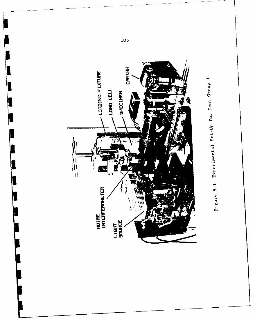
1 105
IL 000
weI.6.0IZ
Immm
106
Figures 6.2 and 6.3 show typical moire interferometry
fringe patterns for specimens No. SB-i and No. SB-4 at
different loading levels. The estimated microcrack tip of
the fracture process zone is marked on each figure. The
fracture process zone in those two specimens extended from
the tip of the machined notches at angles of 40 and 30
degrees, respectively, to the axes of the notch. The
inclined fracture process zone was caused by aggregates
which were located approximately 2-3 millimeters below the
surface to which the active grating, or specimen grating,
was attached. The locations of those aggregates are
identified by the dotted lines in Figure 6.2 and 6.3. The
microcrack tip location after being projected onto the net
section of the specimen, was used to determine the amount
of crack extension for a given increase in load. The order
of the moire fringes was used to determine the crack
opening displacement (COD) variations along the fracture
process zone.
The data points in Figures 6.4 and 6.5 represent the
COD variation along the fracture process zone at different
load levels for specimen Nos. SB-l and SB-4, respectively.
These loads are for increasing applied displacements and
they occurred under decreasing applied load in the strain
softening regime. The increasing COD at the relatively
blunt notch tip with increasing applied displacement but
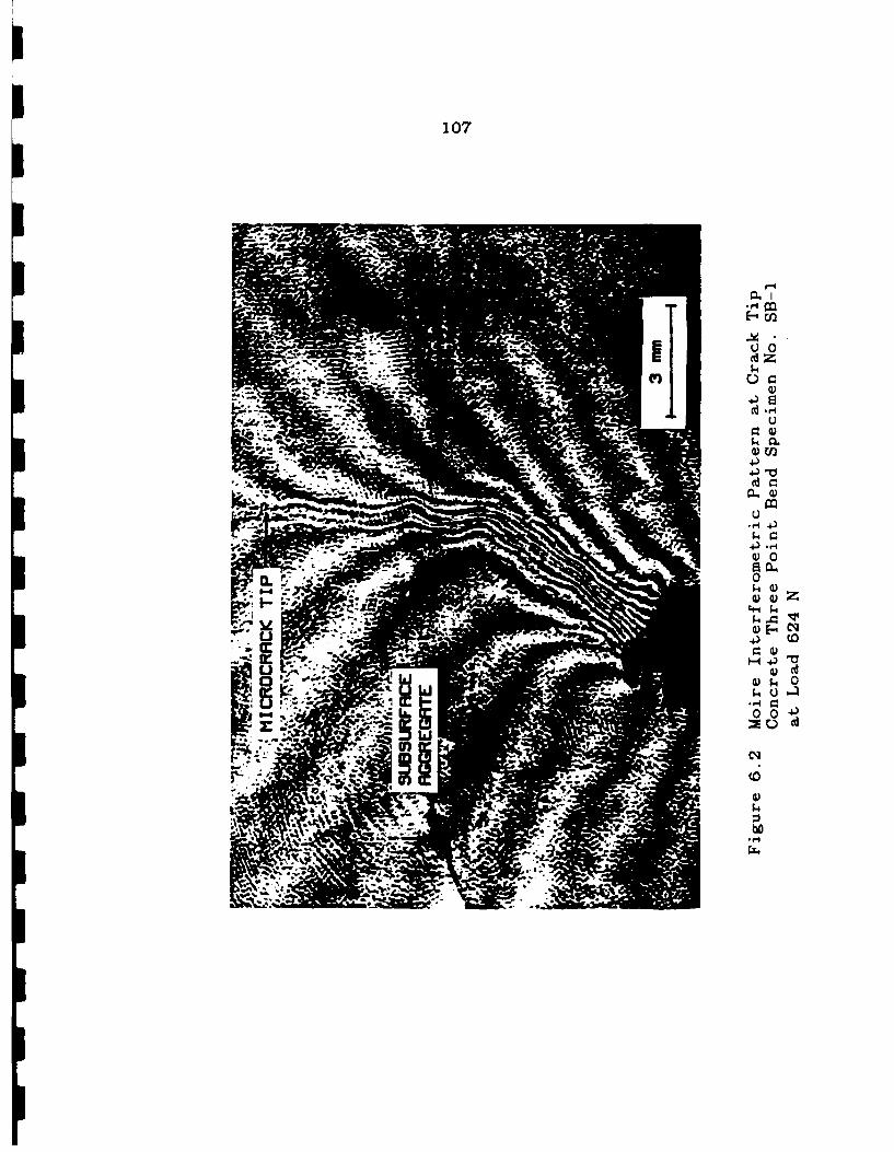
107
S0
&40
Cq
bo C

108
E-4
u
4O
bflcZ4
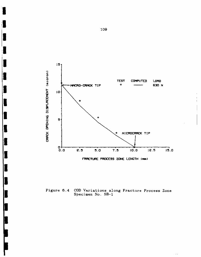
109
I 15,
TEST COMPUTED LOAD
0z 0
V 0 M I CROC TIPKaT I PU
0.0 e.5 5.0 7.5 10.0 1e'.5- 15.0
FRCUE PROCESS ZONE LENGTH (aMM)
i Figure 6.4 COD Variations along Fracture Process Zone
Specimen No. SB-I
PlUC
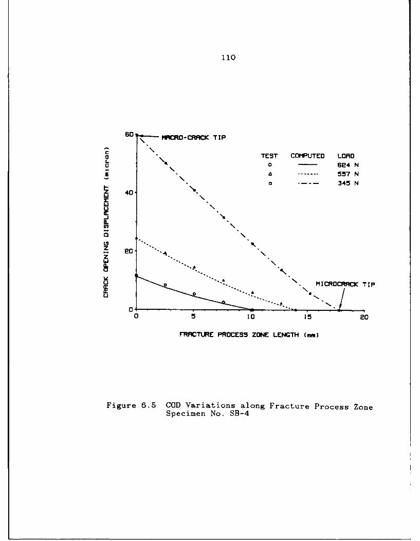
110
r'1 - PW1RO -CFW:1CK TIP
o TEST COMPUTED LORDO o0 6e4 N
a ------ 557 N
a -345 N
40-
U-j "
00.
S N. SB-4
FRACTURE PROCESS ZONE LNT
Figure 6.5 COD Variations along Fracture Process ZoneSpecimen No. SB-4
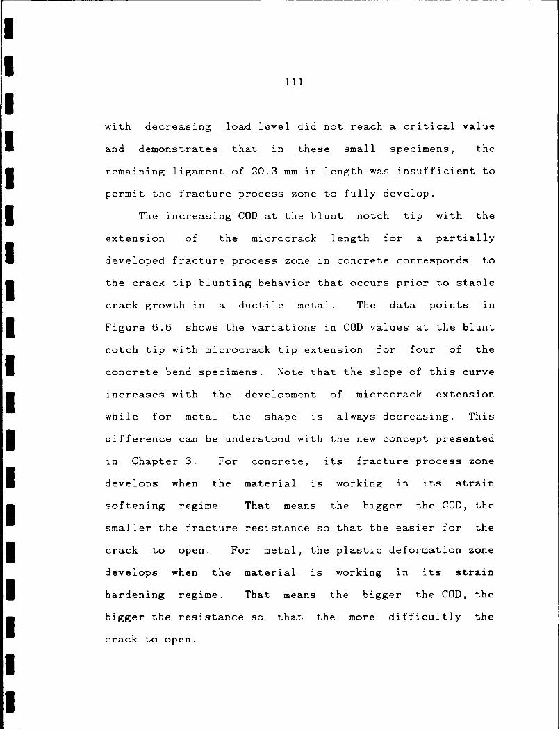
I111
Iwith decreasing load level did not reach a critical value
I and demonstrates that in these small specimens, the
3 remaining ligament of 20.3 mm in length was insufficient to
permit the fracture process zone to fully develop.
3 The increasing COD at the blunt notch tip with the
extension of the microcrack length for a partially
I developed fracture process zone in concrete corresponds to
3 the crack tip blunting behavior that occurs prior to stable
crack growth in a ductile metal. The data points in
SFigure 6.6 shows the variations in COD values at the blunt
notch tip with microcrack tip extension for four of the
I concrete bend specimens. Note that the slope of this curve
3 increases with the development of microcrack extension
while for metal the shape is always decreasing. This
3 difference can be understood with the new concept presented
in Chapter 3. For concrete, its fracture process zone
I develops when the material is working in its strain
softening regime. That means the bigger the COD, the
smaller the fracture resistance so that the easier for the
3 crack to open. For metal, the plastic deformation zone
develops when the material is working in its strain
U hardening regime. That means the bigger the COD, the
* bigger the resistance so that the more difficultly the
crack to open.
I
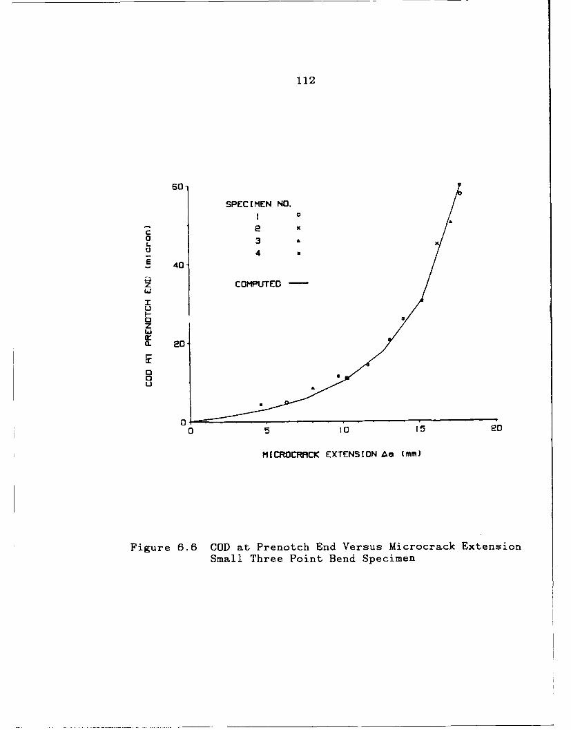
112
60-
SPECIMEN NO.
10
i. 3U 4 U
! 40-
z COMPUTED-
U
z
0. 20-1-
0U
0 5 1O I5 20
MICROCRACK EXTENSION As (mm)
Figure 6.6 COD at Prenotch End Versus Microcrack ExtensionSmall Three Point Bend Specimen
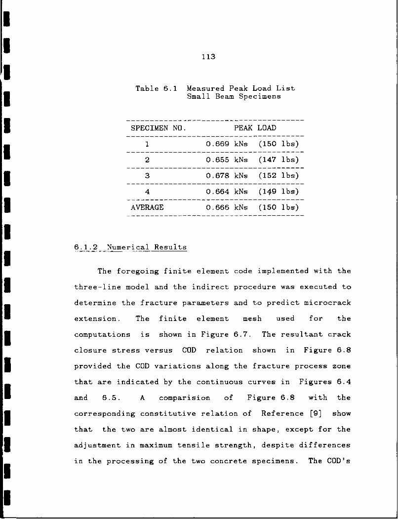
113
Table 6.1 Measured Peak Load ListSmall Beam Specimens
|- - - - - - - - - - - - - - - - - - - -SPECIMEN NO. PEAK LOAD
1 0.669 kNs (150 lbs)
2 0.655 kNs (147 lbs)- 3 0.678 kNs (152 ibs)
4 0.664 kNs (149 lbs)
3 AVERAGE 0.666 kNs (150 lbs)
6.1.2 Numerical Results
The foregoing finite element code implemented with the
3 three-line model and the indirect procedure was executed to
determine the fracture parameters and to predict microcrack
extension. The finite element mesh used for the
3computations is shown in Figure 6.7. The resultant crack
closure stress versus COD relation shown in Figure 6.8
3 provided the COD variations along the fracture process zone
that are indicated by the continuous curves in Figures 6.4
and 6.5. A comparision of Figure 6.8 with the
3 corresponding constitutive relation of Reference [9] show
that the two are almost identical in shape, except for the
3 adjustment in maximum tensile strength, despite differences
in the processing of the two concrete specimens. The COD'sI
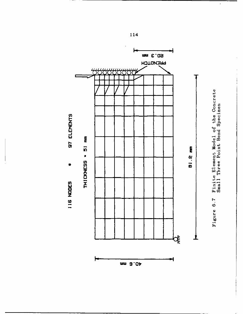
114
WWa c ,oB
HO.LONMd
4
u
0O0)
4-)
-4-Li r.4
0 4-4-E
zCo _ -
Li r--4w ~c/
44a
.14
WW 9,01
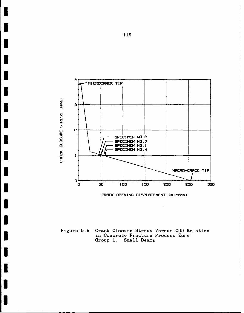
II
115II
M IRORRKT I P
Iw
U2
o~~PC TE I P NO
u SPECIMEN NO.2
LISECIMEN NO.!
013 0 50 00 150 200 250 300
CRACK OPENING DISPLACEMENT (micron)II
Figure 6.8 Crack Closure Stress Versus COD Relationin Concrete Fracture Process ZoneGroup 1. Small Beams
I
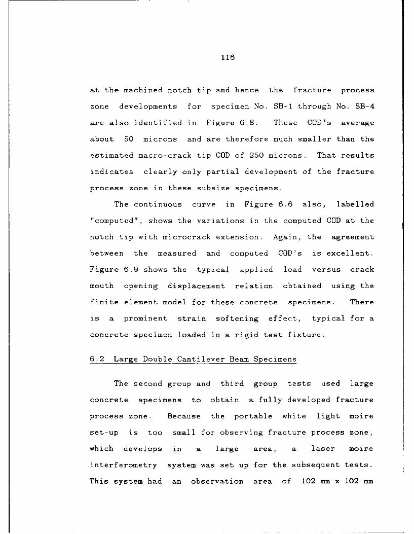
116
at the machined notch tip and hence the fracture process
zone developments for specimen No. SB-i through No. SB-4
are also identified in Figure 6.8. These COD's average
about 50 microns and are therefore much smaller than the
estimated macro-crack tip COD of 250 microns. That results
indicates clearly only partial development of the fracture
process zone in these subsize specimens.
The continuous curve in Figure 6.6 also, labelled
"computed", shows the variations in the computed COD at the
notch tip with microcrack extension. Again, the agreement
between the measured and computed COD's is excellent.
Figure 6.9 shows the typical applied load versus crack
mouth opening displacement relation obtained using the
finite element model for these concrete specimens. There
is a prominent strain softening effect, typical for a
concrete specimen loaded in a rigid test fixture.
6.2 Large Double Cantilever Beam Specimens
The second group and third group tests used large
concrete specimens to obtain a fully developed fracture
process zone. Because the portable white light moire
set-up is too small for observing fracture process zone,
which develops in a large area, a laser moire
interferometry system was set up for the subsequent tests.
This system had an observation area of 102 mm x 102 mm
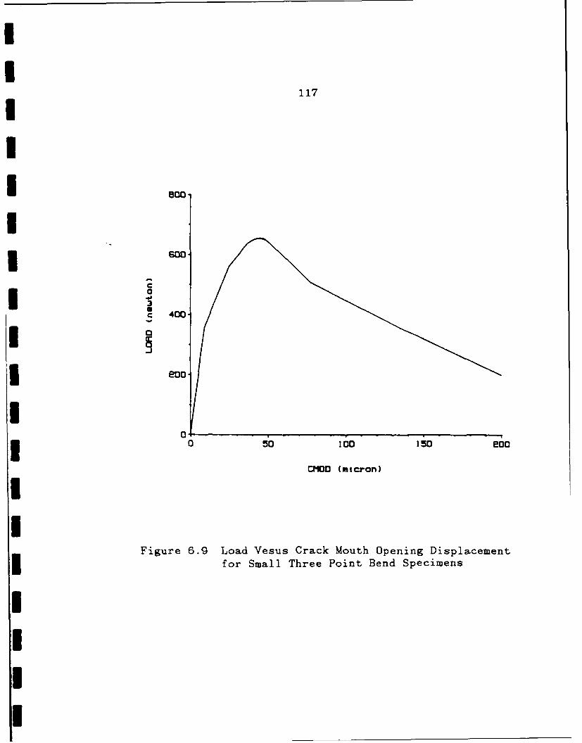
117
Ic
* 00
I3S400
iC
D-
0
0 160 I oi eoo
CMOD (m0cron)
I
Figure 6.9 Load Vesus Crack Mouth Opening Displacementfor Small Three Point Bend Specimens
I!0I!_ _ _ _ _ _ _ __ _ _ _ _ _ _ _ _
3 0lo s 0
118
(4 in. x 4 in.). The numerical analysis used for these
groups was also the indirect finite element method with
three-line model.
6.2.1 Experimental Results
Two large identical specimens for Group 2 and two
large identical specimens for Group 3 were tested using a
shop press. The difference between these Groups is the
maximum aggregate size. The maximum aggregate size of
Group 2 is 6.3 mm and that of Group 3 is 9.5 mm. The crack
opening of each specimen was detected by moire
interferometry. Figure 6.10 shows the test setup and one
of the specimens during the test. The specimen dimensions
have already been given in Figure 4.1 in Chapter 4.
The wedge load, the crack mouth opening displacement
2V and the crack tip opening displacement 2V2 were
recorded by a HP computer. Figures 6.11 and 6.12 show the
test results of the wedge load versus 2V1 curves by
continuous lines for Group 2 and Group 3 specimens,
respectively. Considerable aggregate size effect can be
seen by comparing these two figures, while the results from
the same material are consistent. The peak load for Group
3 is about 25% larger than that for Group 2. Figures 6.13
and 6.14 show the measured 2V2 versus 2V curves also by
continuous curves for Group 2 and Group 3 specimens,

I
I
I
II
IqIId
I
i Figure 6.10 Experimental Set-Up for Test Group 2,3.
Ii
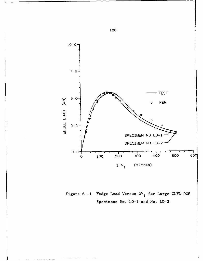
120
10.0-
7.5-
- TEST
5.0--Xo FEM
C0
2.5
SPECIMEN NO.LD-1
SPECIMEN NO.LD-2
0 100 200 300 400 500 600
2 V1 (micron)
Figure 6.11 Wedge Load Versus 2V 1 for Large CLWL-DCB
Specimens No. LD-1 and No. LD-2
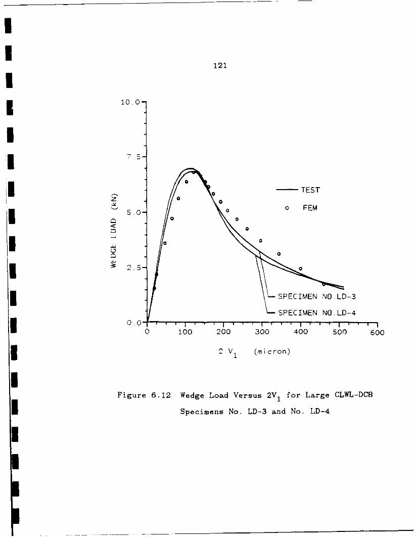
121
10.0-
I
1 75
zI 0TEST
5.0 0 FEM
0 0
*0
~ 2.5,
SPECIMEN NO.LD-3
SPECIMEN NO.LD-40 .0- . . . - I I I I I I' ' I -I
0 100 200 300 400 500 600
3 V1 (micron)
IFigure 6.12 Wedge Load Versus 2V 1 for Large CLWL-DCB
Specimens No. LD-3 and No. LD-4I'
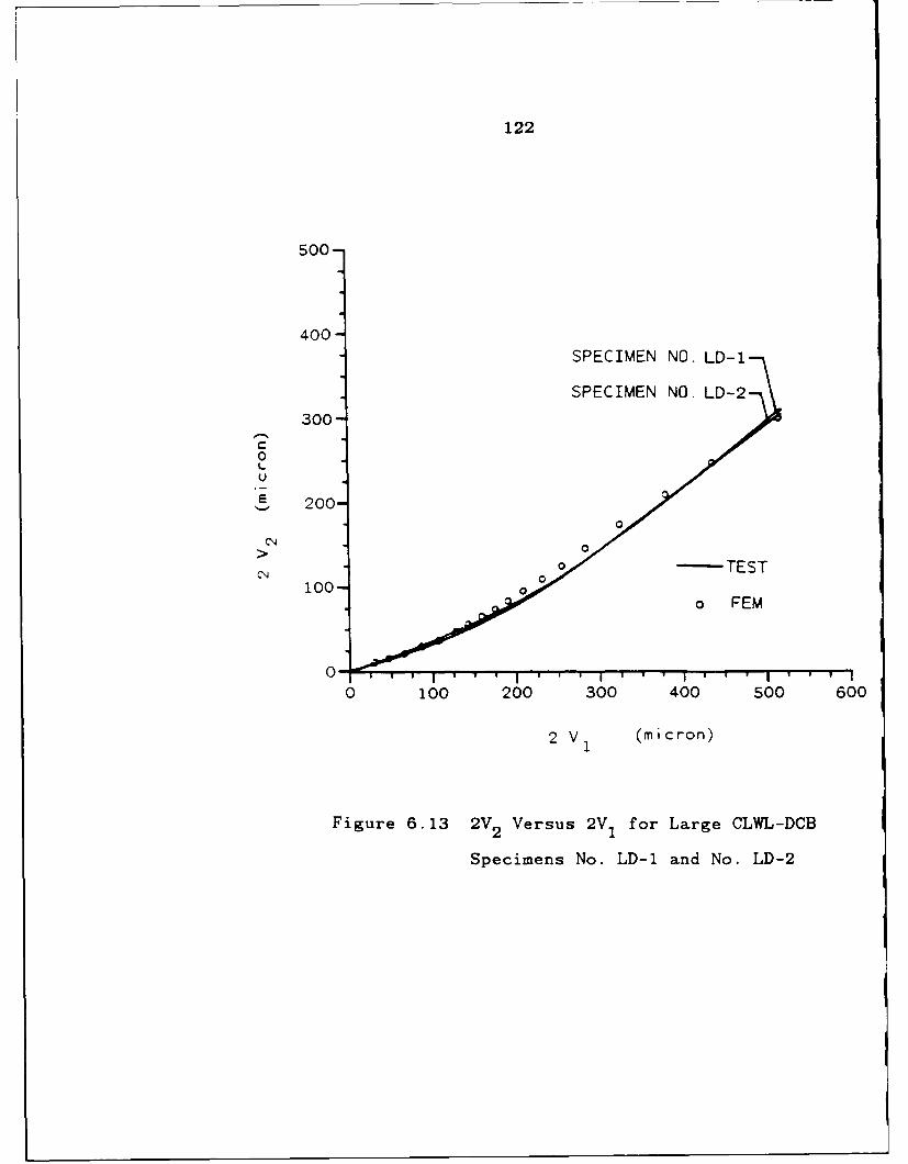
122
500-
400-SPECIMEN NO. LD-1
SPECIMEN NO. LD-2
300-c0IU
200-0
0 -TEST100 0
0 FEM
0-0 100 200 300 400 500 600
2 V 1 (micron)
Figure 6.13 2V 2 Versus 2V I for Large CLWL-DCB
Specimens No. LD-1 and No. LD-2
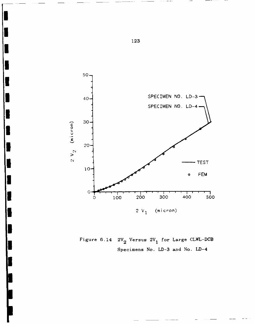
123
I50,
I40- SPECIMEN NO. LD-3
SPECIMEN NO. LD-4
i- 30
0U IU°E
3 20.
TEST
10-- 0 FEM
0- " ' °'
0 100 200 300 400 500
3 2 V, (micron)
IFigure 6.14 2V2 Versus 2V 1 for Large CLWL-DCB
Specimens No. LD-3 and No. LD-4
I
124
respectively. There is no big difference between the
results of these COD relations of these two groups.
Moire interferometry fringe patterns were photographed
and then evaluated to obtain the crack length and crack
opening displacement along the fracture process zone.
Difficulty was encountered when the observation area became
as large as 102 mm x 102 mm. The home-made diffraction
gratings of this size produced too many initial fringes in
the null patterns when these groups tests were conducted.
The null pattern was superimposed on the fringe patterns
associated with the deformation of the specimen. Although
subtraction of the null pattern was possible, the necessary
software, which is a state of art in computer :ience, was
not available.
Fortunately, the determination of the crack opening
displacement does not require the absolute displacement of
the entire field and only the relative displacement between
the two corresponding points of the opposite crack surfaces
is needed. This relative displacement is the COD and was
evaluated by counting the fringes along the crack surfaces.
The continuous lines in Figures 6.15 and 6.16 represent the
measured crack opening displacement along the fracture
process zone for Groups 2 and 3, respectively.
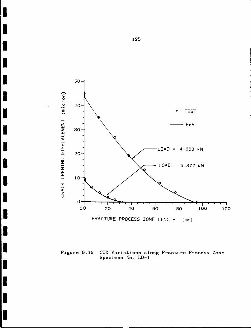
125
I.
o
I0. U 40-
E o TEST
FEMS30-
I0 LOAD = 4.663 kN20.
-LOAD = 6.372 kNZ,WCL.
M 10-
U0-CO 20 40 60 80 100 120
FRACTURE PROCESS ZONE LENGTH (mm)
Figure 6.15 COD Variations along Fracture Process ZoneSpecimen No. LD-1
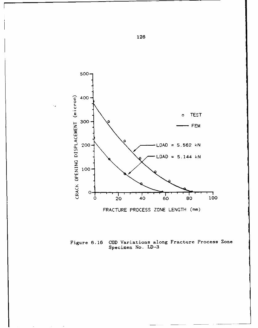
126
500-
C 4000LU
E o TEST
300-z3 . - FEM
LU
LU
<- O 200- LOAD = 5.562 kN
LOAD = 5.144 kN
zz 100-LUI
< 0-0 20 40 60 80 100
FRACTURE PROCESS ZONE LENGTH (mm)
Figure 6.16 COD Variations along Fracture Process ZoneSpecimen No. LD-3
I
127I6.2.2 Numerical Results
The nonlinear finite element analysis was then
I conducted for finding the fracture model for these
specimens. The finite element model is shown in
Figure 6.17. The wedge load applied to the hole surface
3 was simplified to a concentrate force. Through extensive
trial and error, fracture models of crack closure stress
versus COD relation were obtained for these two groups and
5 are shown in Figures 6.18 and 6.19. Based on these models,
various specimen behaviors were predicted. The data points
in Figure 6.11 through Figure 6.16 represent the numerical
results of the experimental counterparts. Good agreements
I were obtained between the test measurements and the
* theoretical predictions.
6.3 Specimens of Adequate Size
It was found that even the moire interferometry
U measuring area had been increased to 102 mm x 102 mm it was
* still far from being large enough for a fully developed
fracture process zone in those large CLWL-DCB specimens
5 used in Groups 2 and 3. Larger moire set-up was not
available. However, since the fracture process zone size
I depends on the specimen geometry and size, fully developed
fracture process zones can be generated which fit the
U
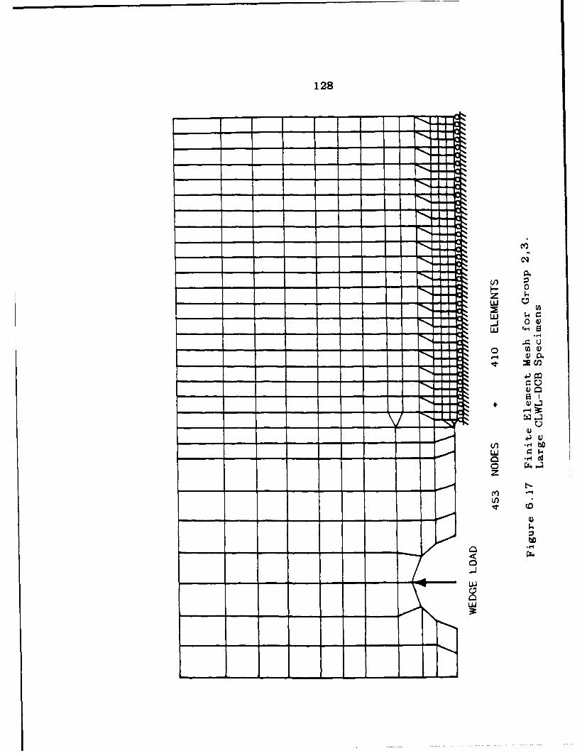
128
___- - - -- -
- - - - -
- - 0
- - --$4
zzc
OG)- - -- - - - - - Lii 442
- -- - - - - -
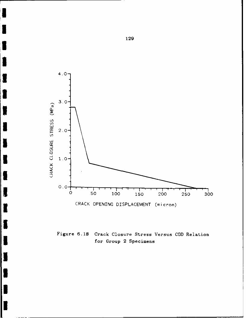
129
* 4.0
i3.0
03 LU= 2.0-
I U
I0.050 50 100 150 200 250 300
CRACK OPENING DISPLACEMENT (micron)
Figure 6.18 Crack Closure Stress Versus COD Relation
3 for Group 2 Specimens
I3IU
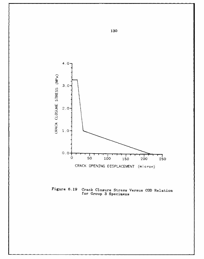
130
4.0-
C.
3.0(A
LU'
1 0-
0.0
0 50 100 150 200 250
CRACK OPENING DISPLACEMENT (micron)
Figure 6.19 Crack Closure Stress Versus COD Relationfor Group 3 Specimens
131
available optical set-up. Thus, finite element experiments
were conducted to arrive at reasonable dimensions for
CLWL-DCB specimen used for Group 4 and for three point bend
specimen used for Group 5. The dimensions of these
specimens are given in Figure 4.2. in Chapter 4. The
laser moire interferometry with a real reference grating
and the direct finite element numerical procedure with the
one-curve model were used in these studies.
6.3.1 Experimental Results
A total of four CLWL-DCB specimens and four three
point bend specimens were loaded nearly to complete
penetration of micro-crack tip of the fracture process
zone. The photographs of the test set-up and the specimens
are given in Figures 6.20, 6.21 and 6.22. The measured
wedge load versus 2V1 and 2V2 versus 2V curves for the
four CLWL-DCB specimens are shown in Figures 6.23 and 6.24.
The load versus load point deflection curve for four three
point bend specimens are shown in Figure 6.25.
Moire interferometry data showed that the fracture
process zone started to develop much earlier than the peak
load was reached. Thus the maximum load that a concrete
specimen can carry without the fracture process zone is
only about 30% to 40% )f the load-carrying capacity of a
concrete specimen with a developed fracture process zone.
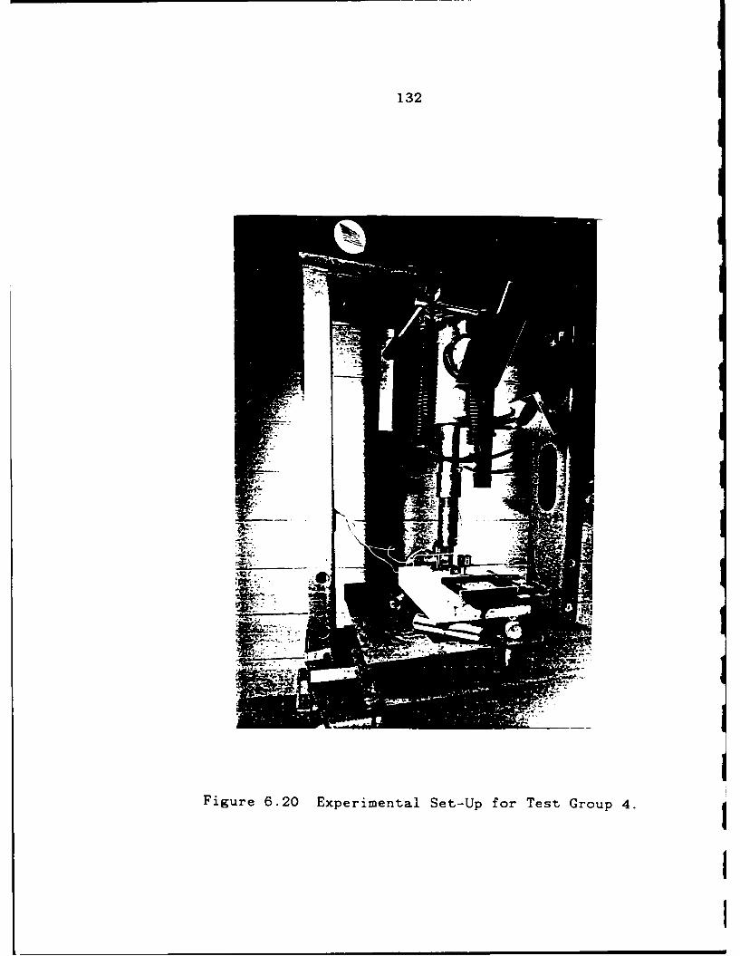
132
Figure 6.20 Experimental Set-Up for Test Group 4.
II,1
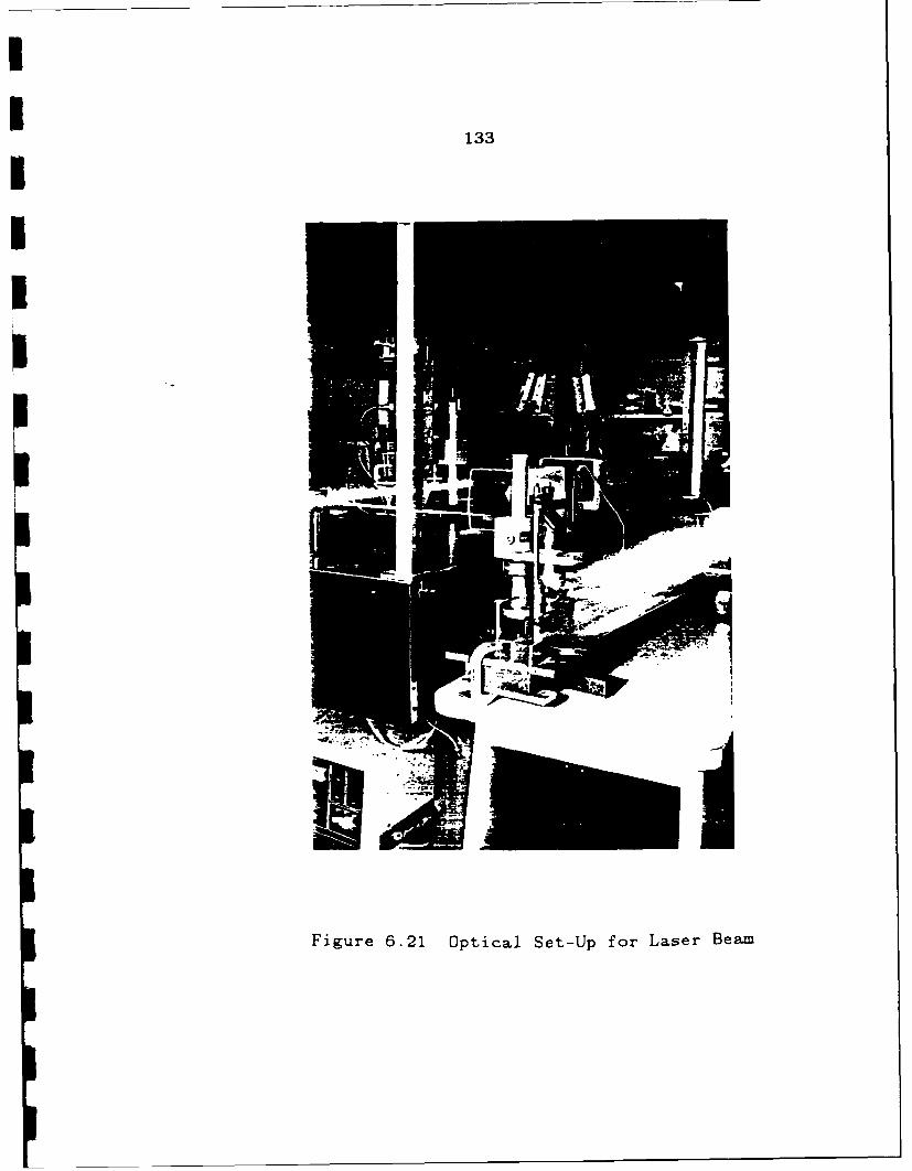
II
133
IIi
II
Fi u e 62 p i a Se-U fo rsr B a
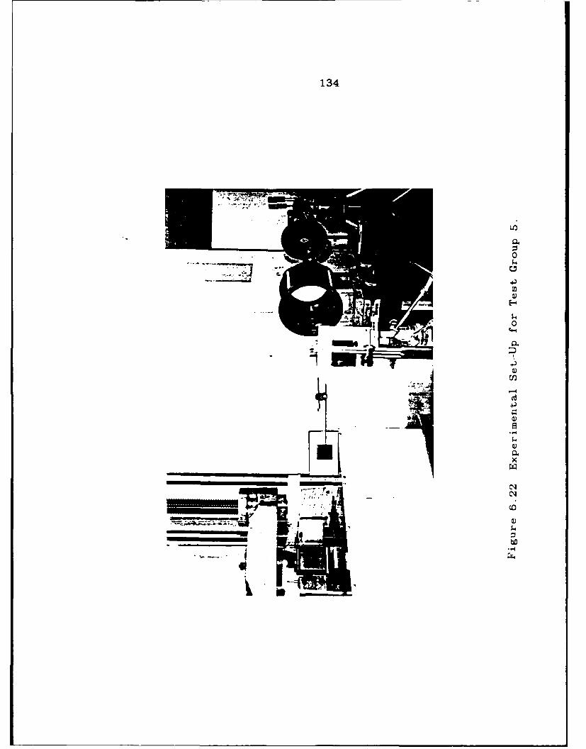
134
0O
0
S-4
4Y,
to
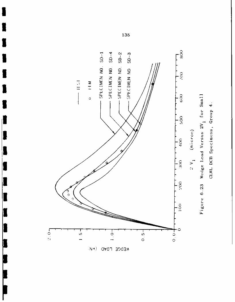
135
Iz z z zLU Lu w
wU LUJCL C-L-1 - - ~ -4
0
L
S E >
Ilye bC
I IU--z
0.N~l T 0 -13003
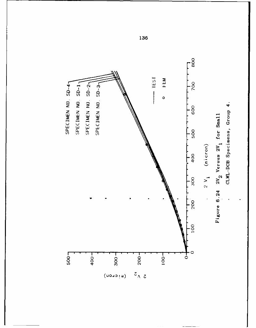
136
04 Cf)
0LU C :
z z z Z0Z z Z 0UJ wU Lu Lu r-4 0
o~ ~~ P-4 0~
L/ l Lf () 0 C
C 91 U)
E 0
C 4
bO.,
1 0
(uoj 0 1W) AN
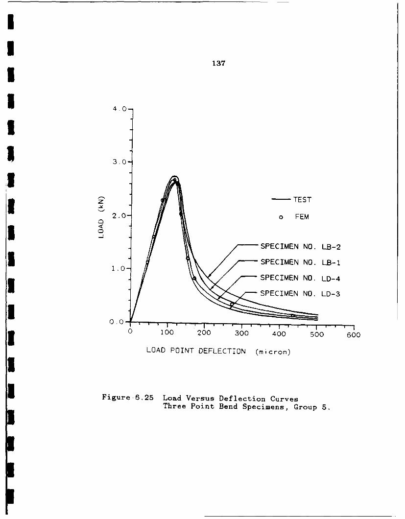
I137
I
1 4.0-
I
3.0
z "TEST
2.0- o FEM
SPECIMEN NO. LB-2
3 SPECIMEN NO. LB-i1.0
SPECIMEN NO. LD-4
SPECIMEN NO. LD-3
0 100 200 300 400 Soo 600
LOAD POINT DEFLECTION (micron)
Figure.6.25 Load Versus Deflection CurvesThree Point Bend Specimens, Group 5.
138
After the peak load, the load decreased while the fracture
process zone continued to extend. The moire fringe
patterns data showed that a fully developed fracture
process zone was achieved when the critical COD of
250 microns was reached.
Figures 6.26 and 6.27 show typical sequentially
recorded moire interferometry fringe patterns for the
CLWL-DCB specimen No. SD-2 and the three-point bend
specimen No. LB-i at different load levels. These fringes
are displacement contours of 1/1200 mm intervals in the
direction of perpendicular to the prenotches.
The order of the moire fringes was used to determine
the COD's variation along the fracture process zone. The
continuous curves in Figures 6.28 and 6.29 represent the
COD variations along the fracture process zone at different
load levels for the CLWL-DCB specimens No. SD-2 and
No. SD-4. The continuous curves in Figures 6.30 and 6.31
represent the COD variations along the fracture process
zone at different load levels in the three point bend
specimens No. LB-4 and No. LB-i, respectively.
All moire patterns showed that the fracture process
zone is not wide as three times aggregate size as
postulated by others [60]. Instead, one aggregate size may
be a better representation of the fracture process zone
width. Similar observation was also obtained in the
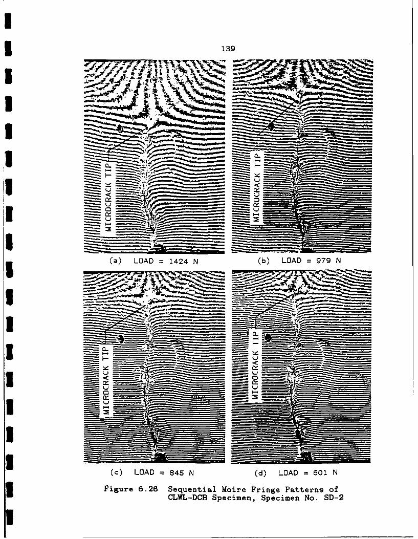
3 139
I 77I XIj ;
Vol* 4;I ik
CL_ __ _
~a7-Q7' _ _ _ _ _ _ _ _
I Q ~ '125
(a) LOA 142 N b)LAD97
Za
- S .J * ~ -will
(a) LOAD 8 424 N (b) LOAD 6097 N
C-L-C Spcmn Spcie No. S-
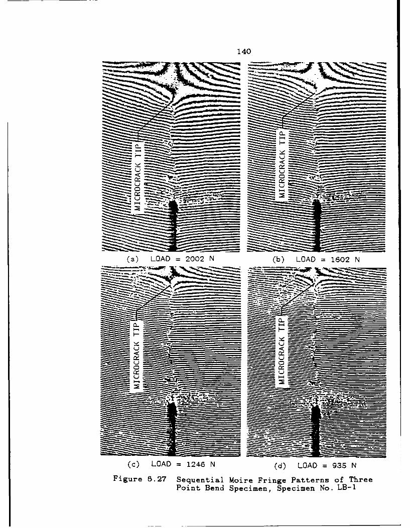
140
PAW-m
(a) LOAD =2002 N (b) LOAD =1602 N
I I . .I I.-I.
........ cc__ . ~ - ~ - - .. ~ - _ _ _ _
(c)~ i ~ LOA 124 N- (d)- LOAD_935_NFigure-- 6.2_SquntalMoreFrngPttrnoTre
Point ~ BenSpcimn,_pecmenNo.__-
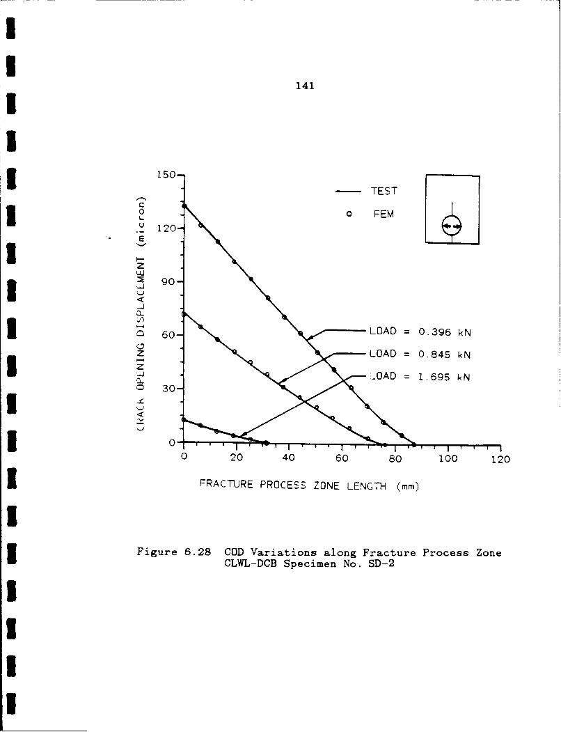
141
150
TESTC I0 FEML
u 120-E
zo-S90-
I<S 0 LOAD = 0.396 kN
0z LOAD = 0.845 kNI z-Lj LOAD = 1.695 kN© 30-
II3 0~
0 20 40 60 80 100 120
3 FRACTURE PROCESS ZONE LENGTH (mm)
IFigure 6.28 COD Variations along Fracture Process Zone
CLWL-DCB Specimen No. SD-2
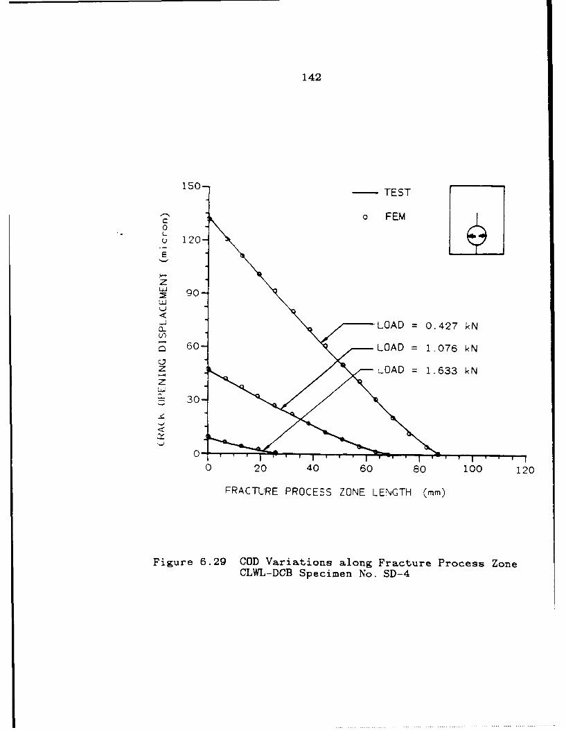
142
150] -TEST
C o FEM0L
u 120E
zS90-
-LOAD = 0.427 kN
60- LOAD = 1.076 kN
z _OAD = 1.633 kN
- 30-
0-I
0 20 40 60 80 100 120
FRACTURE PROCESS ZONE LENGTH (mm)
Figure 6.29 COD Variations along Fracture Process ZoneCLWL-DCB Specimen No. SD-4
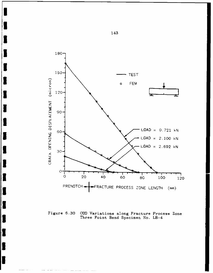
1I
143I5180-
O150- TEST
0oo FEMU
I -e~ 120 -3Ez
LU 90
I<
0- LOAD = 0.721 kNI o 60-
z LOAD = 2.100 kNZ
30_ LOAD = 2.692 kN-30-
010 20 40 60 80 100 120
PRENOTCH +fFRACTURE PROCESS Z ONE LENGTH (mm)
IFigure 6.30 COD Variations along Fracture Process Zone3 Three Point Bend Specimen No. LB-4
I
I!
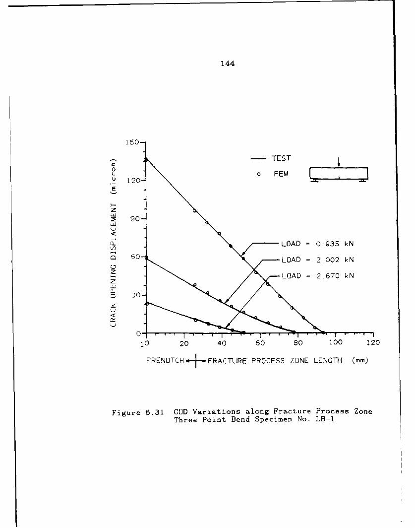
144
150-
- TEST
L o FEMu 120-
E
z
S90"
CL)LOAD = 0.935 kN
60-- LOAD = 2.002 kN
z-LOAD = 2.670 kNz
z 30-4::
0 -
10 20 40 60 80 100 120
PRENOTCHjFRACTURE PROCESS ZONE LENGTH (mm)
Figure 6.31 COD Variations along Fracture Process ZoneThree Point Bend Specimen No. LB-1
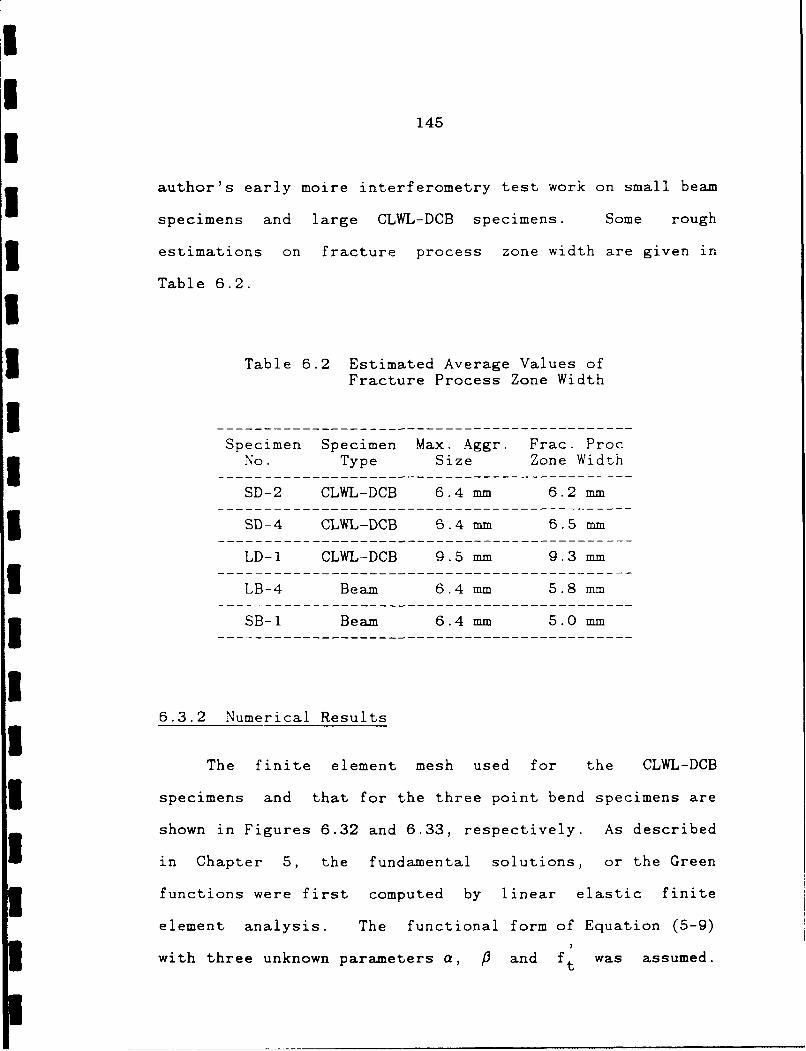
I
145
author's early moire interferometry test work on small beam
specimens and large CLWL-DCB specimens. Some rough
3 estimations on fracture process zone width are given in
Table 6.2.I
STable 6.2 Estimated Average Values ofFracture Process Zone Width
-Specimen Specimen Max. Aggr. Frac. Proc3 No. Type Size Zone Width
SD-2 CLWL-DCB 6.4 mm 6.2 mm
SD-4 CLWL-DCB 6.4 mm 6.5 m
LD-I CLWL-DCB 9.5 mm 9.3 mm
I LB-4 Beam 6.4 mm 5.8 mm
3 SB-I Beam 6.4 mm 5.0 mm
-6.3.2 Numerical Results
The finite element mesh used for the CLWL-DCB
specimens and that for the three point bend specimens are
shown in Figures 6.32 and 6.33, respectively. As described
in Chapter 5, the fundamental solutions, or the Green
functions were first computed by linear elastic finite
element analysis. The functional form of Equation (5-9)
with three unknown parameters a, P and ft was assumed.
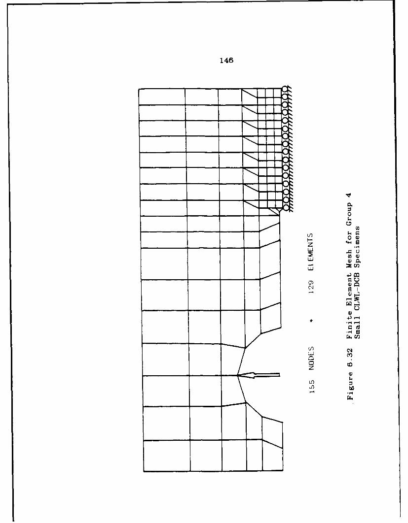
146
00)
CLJ
0/)
0 CzLO)
-4D

147
I HDION38d
0ou
I LLULU
I - -
C4 4 Q
Q)Ina
z
I bD.m

148
The resulting fundamental solutions were stored on a hard
disc and later retrieved by another program which is used
to determine the three unknown parameters in the crack
closure stress versus COD relation which optimally
satisfied the input experimental results of COD along the
fracture process zone, load, 2V1 and 2V2 for the CLWL-DCB
or load point displacement for the three point bend
specimens.
The above generation phase of analysis was carried out
twice using the test data of a CLWL-DCB specimen No. SD-2
and a three point bend specimen No. LB-4, respectively.
The same resultant crack closure stress versus COD curve,
as shown in Figure 6.34, for these two types of specimen
was obtained through this hybrid experimental-numerical
analyses. This relation also agrees well with the results
of direct tension tests [12,42,103,104] as shown in
Figure 6.35. The area under this curve is estimated to be
107 N/M, which is reasonably close to the work of fracture
reported by others [46]. Also, the previously developed
three-line model through the trial and error procedure was
used to check the validity of the direct procedure and the
function assumed. Good agreements in the general shape and
the area, which is shown in Figure 6.36, were obtained.
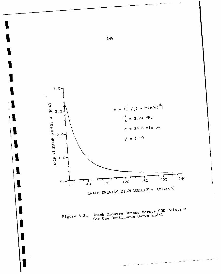
149
I 4.0
=T f + 2(/f
~3.0
f= 3.24 MPa
= 34.3 micron
p=50
I 0
4. 00 80 120 160 2400 240
CRACK. OPENING DISPLACEMENT w (micron)
Figure 6.34 Crack Closure Stress Versus COD Relationl
3 for One Cotinluous Curve Model
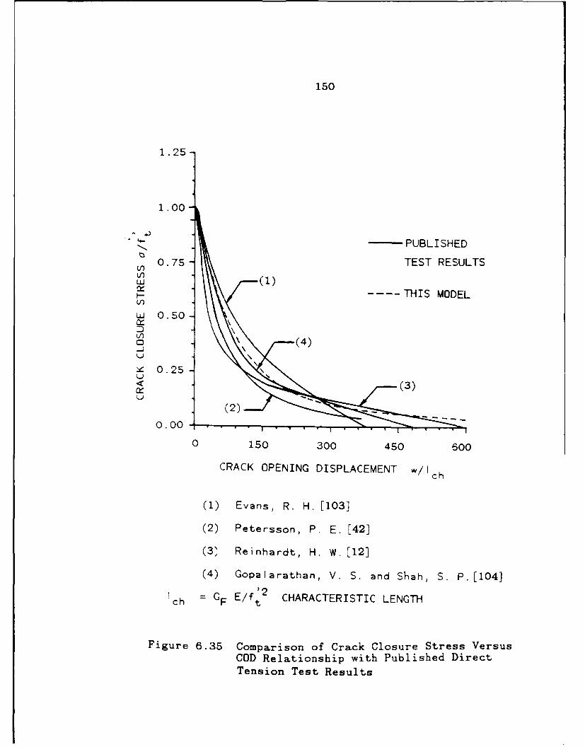
150
1 .25
1.00-
-- PUBLISHED
0.75 TEST RESULTS
LUj (1)---- THIS MODEL
U 0.50
V(4(~(4)
0.25
(3)
(2) -
0.00 .
0 150 300 450 600
CRACK OPENING DISPLACEMENT w/Ich
(1) Evans, R. H. [103]
(2) Petersson, P. E. [42]
(3" Reinhardt, H. W. [12]
(4) Gopalarathan, V. S. and Shah, S. P.[104]
ch = GF E/f 2 CHARACTERISTIC LENGTH
Figure 6.35 Comparison of Crack Closure Stress VersusCOD Relationship with Published DirectTension Test Results

151
4.0 -
~,3.0-0'
THREE LINE SEGMENT MODEL
I '2.0-
I THIS MODEL DDEL
<1.0
~~~~0.0 1 U
0 40 80 120 160 200 240
CRACK OPENING DISPLACEMENT (micron)
Figure 6.36 Comparison of Three - Line Model with
One - Curve Model for Group 4,5 specimens
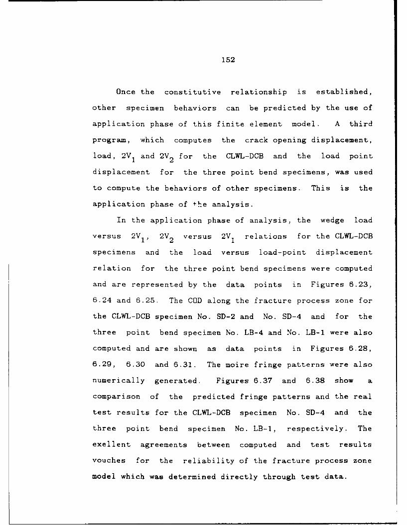
152
Once the constitutive relationship is established,
other specimen behaviors can be predicted by the use of
application phase of this finite element model. A third
program, which computes the crack opening displacement,
load, 2V 1 and 2V 2 for the CLWL-DCB and the load point
displacement for the three point bend specimens, was used
to compute the behaviors of other specimens. This is the
application phase of +he analysis.
In the application phase of analysis, the wedge load
versus 2VI, 2V 2 versus 2VI relations for the CLWL-DCB
specimens and the load versus load-point displacement
relation for the three point bend specimens were computed
and are represented by the data points in Figures 6.23,
6.24 and 6.25. The COD along the fracture process zone for
the CLWL-DCB specimen No. SD-2 and No. SD-4 and for the
three point bend specimen No. LB-4 and No. LB-l were also
computed and are shown as data points in Figures 6.28,
6.29, 6.30 and 6.31. The moire fringe patterns were also
numerically generated. Figures 6.37 and 6.38 show a
comparison of the predicted fringe patterns and the real
test results for the CLWL-DCB specimen No. SD-4 and the
three point bend specimen No. LB-i, respectively. The
exellent agreements between computed and test results
vouches for the reliability of the fracture process zone
model which was determined directly through test data.
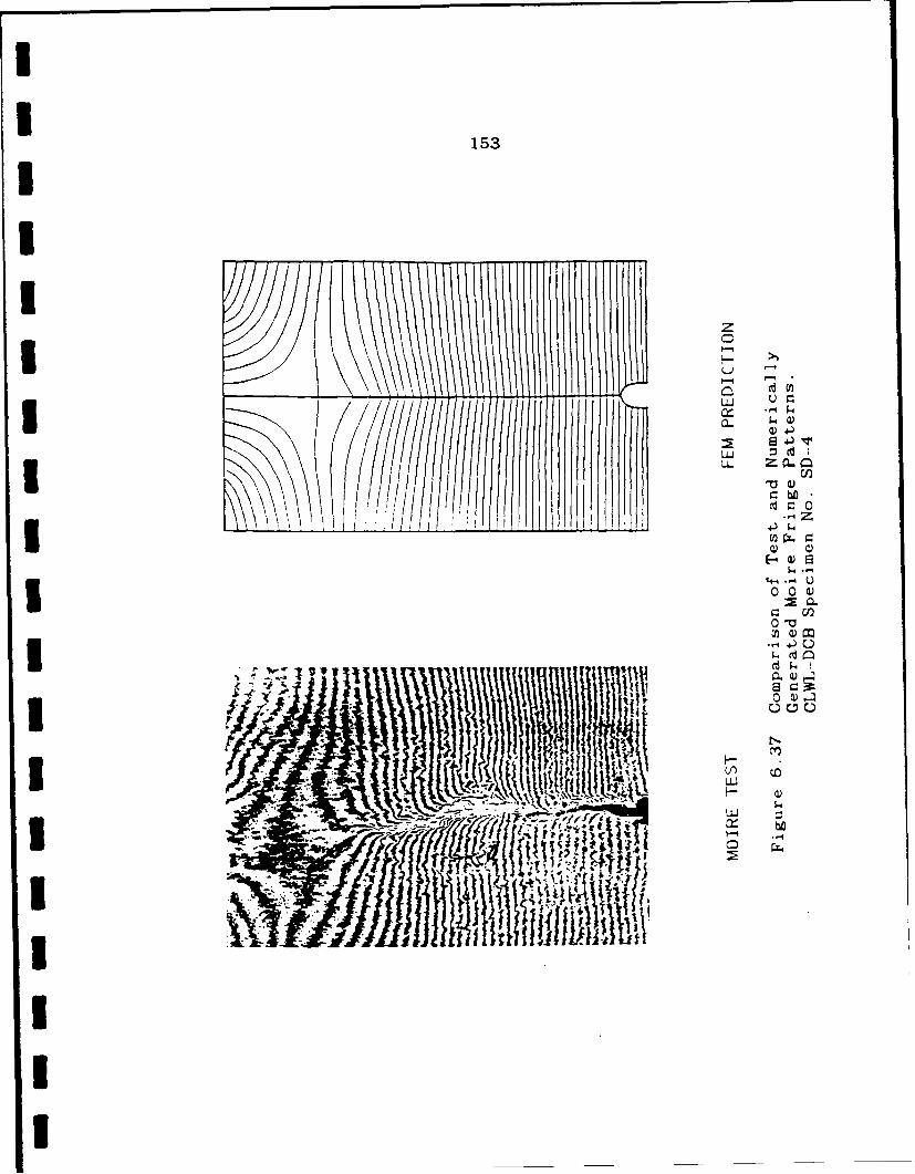
153
I rUL
I -
\ ' ' 4 -1
I .,4.)
.cdC
cd4 ~I CDo0
*gf L12
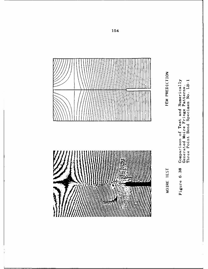
154
z
u C
-)
LU
bO
w~ C
C44 .. 4 M
0 0
0 M -U)0
0 )
II'' ~IIu
00I/4 */A~ m
p ~~4..Jb
I155
IBesides these comparisons, other numerical results
were also obtained which predicted the stress distribution
3 and energy partition. Since these quantities are not
directly measurable, only numerical results were obtained.
3 Figure 6.39 and Figure 6.40 show the normal stress
distributions along the crack paths of CLWL-DCB and three
point bend specimens, respectively. The existence of a
* considerable crack closure stress explains the increase in
the loading capacity by the fracture process zone. Similar
3 stress distributions were obtained for these two types of
specimens. This fact suggests that different overall
stress state need to be created in order to check the
3 stress state dependency of the fracture model.
Figures 6.41 and 6.42 are energy partitions for CLWL-DCB
3 and three point bend specimens, respectively. The strain
energies undergo an increase then decrease while the
fracture energies monotonically increase at increasing
3 rates with respect to the crack extensions. The total
amount of the fracture energy should be equal to the GF
3 times the fracture area, which can be a double check of the
finite element computation.U6.3.3 DiscussionsI
In order to match the test results, a modulus of
3 elasticity, E, was needed for the computations that was
I
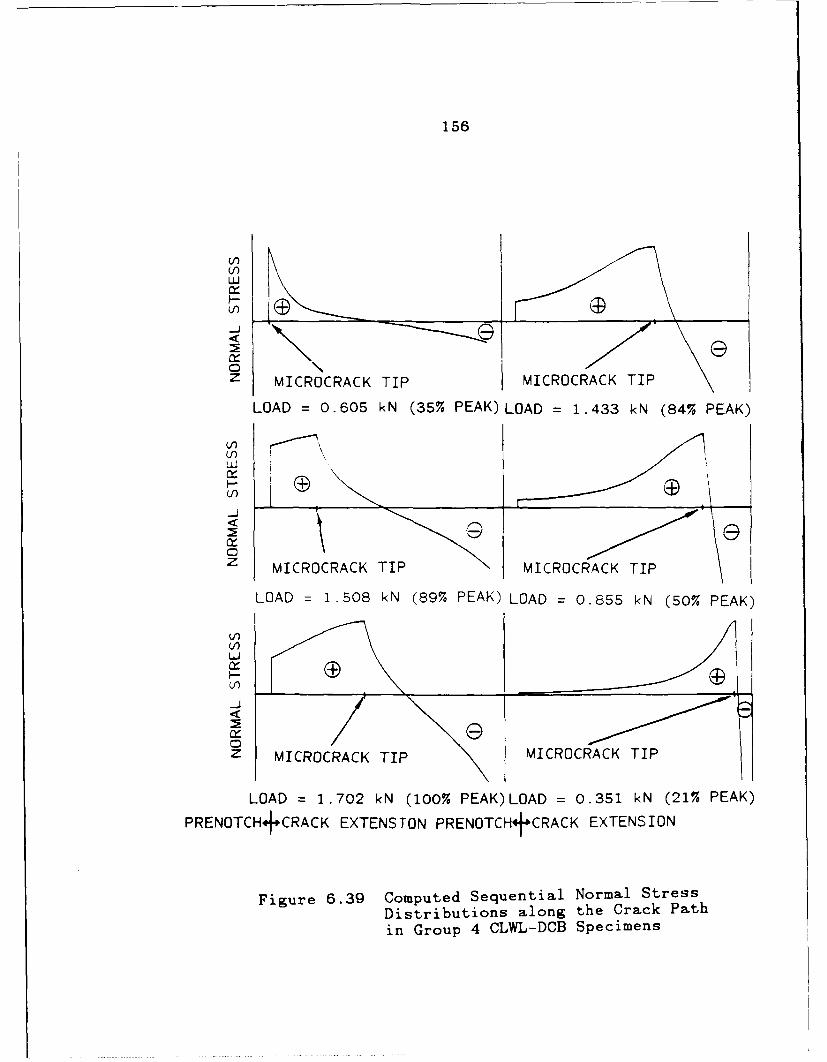
156
U0
Z MICROCRACK TIP MICROCRACK TIP
LOAD = 0.605 kN (35% PEAK) LOAD = 1.433 kN (84% PEAK)
U~1
LII
z TP
Z MICROCRACK TIP MICROCRACK TIP
LOAD 1.508 kN (89% PEAK) LOAD = 0.855 kN (50% PEAK)
U
0
Z MICROCRACK TIP MICROCRACK TIP
LOAD = 1.702 kN (100% PEAK)LOAD = 0.351 kN (21% PEAK)
PRENOTCH+CRACK EXTENSTON PRENOTCHhCRACK EXTENSION
Figure 6.39 Computed Sequential Normal StressDistributions along the Crack Path
in Group 4 CLWL-DCB Specimens
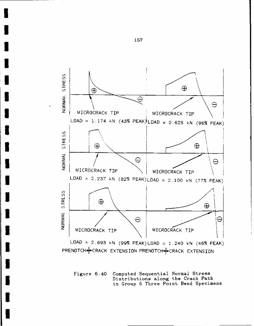
iI
157I
U)
I UjZ MICROCRACK TIP > MICROCRACK TIP
LOAD = 1.174 kN (43% PEAK)LOAD = 2.625 kN (967% PEAK)
I U')I MICROCRACK TIP MICROCRACK TIP
LOAD = 2.237 kN (829% PEAK)LOAD = 2.100 kN (77% PEAK)
II
I MICROCRACK TIP MICROCRACK TIP
I LOAD = 2. 693 kN (99% PEAK) LOAD = 1. 240 kN (46% PEAK)
PRENOTCH+CRACK EXTENSION PRENOTCH+CRACK EXTENSION
IFigure 6.40 Computed Sequential Normal Stress
Distributions along the Crack Pathin Group 5 Three Point Bend Specimens
I
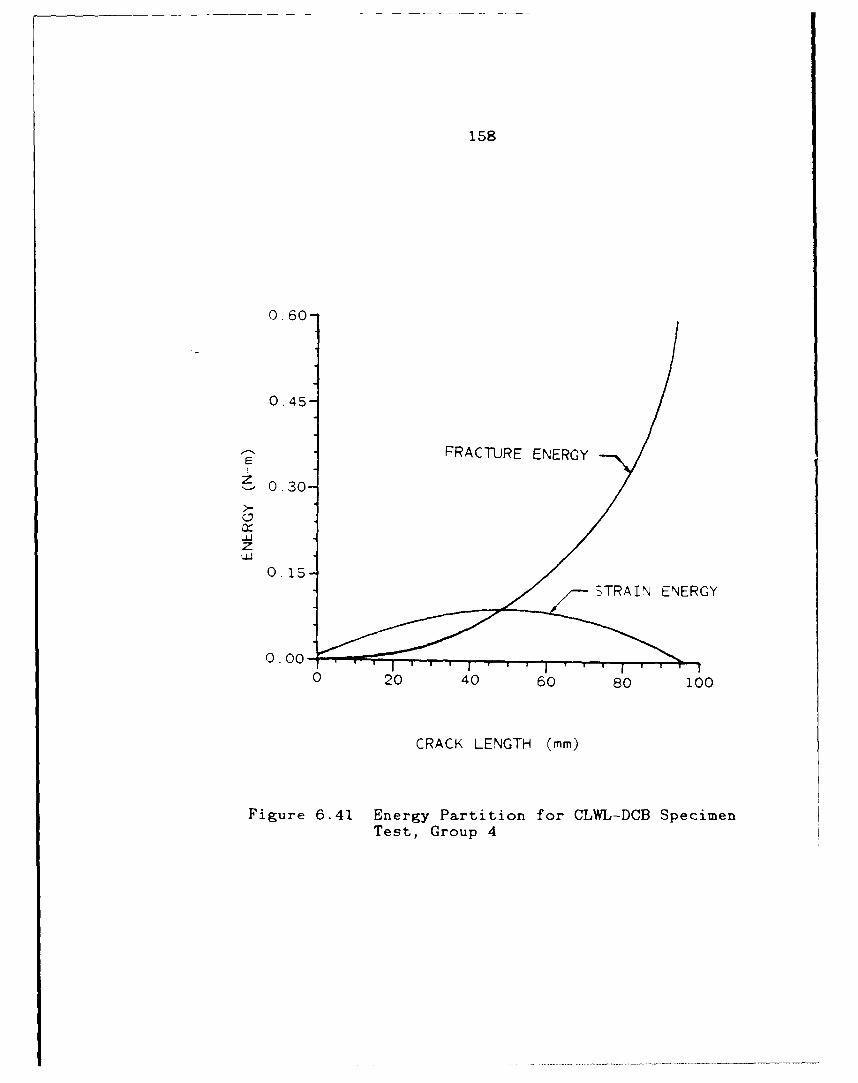
158
0.60-
0.45-
PRACThRE ENERGYE
z
0.15-
STRAIN ENERGY
020 40 60 so 100
CRACK LENGTH (mm)
Figure 6.41 Energy Partition for CLWL-DCB SpecimenTest, Group 4
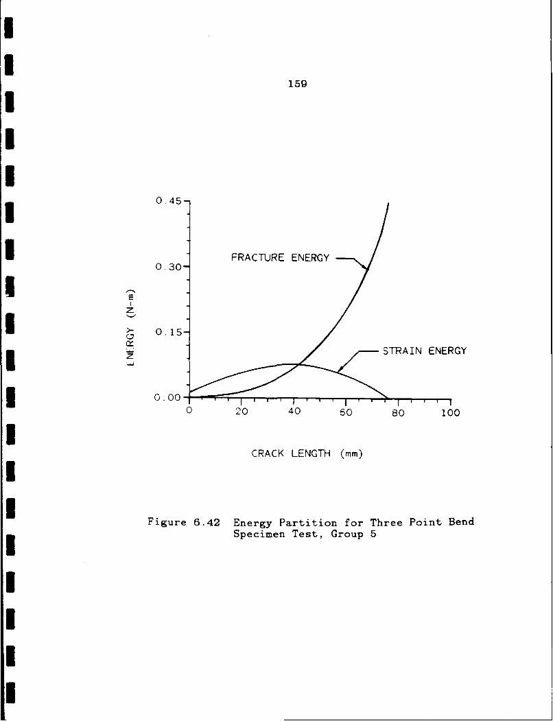
159
I
1 0.45
I FRACTURE ENERGY0.30-
* Ez
Q 0.15-
z-~ STRAIN ENERGY
I ''0.000 20 40 60 80 100
ICRACK LENGTH (mm)I
Figure 6.42 Energy Partition for Three Point Bend
Specimen Test, Group 5
I
160
smaller than the values measured using the small tension
specimens. The use of a smaller modulus of elasticity is
reasonable since the measured E is the tensile tangential
modulus which is smaller than the average slope for the
ascending portion of the stress-strain curve. Furthermore,
these specimens were subjected to both tensile and
compressive loading where the compressive modulus for this
concrete could be 20% smaller [9] than the tensile modulus.
When only one E is used for computations, a smaller modulus
would better represent the average condition than the
initial tensile tangential modulus value.
The tensile strength, ft, was considered as one of the
fracture parameters determined in the optimization
procedure. The resulting tensile strength was slightly
smaller than that measured by the direct tension test, but
is within the range of the variation in material property
and experimental error.
The Poisson's Ratio was assumed to be 0.15 L9]. The
compressive strength was not needed for numerical analysis
because the specimens were designed to fail in tension.
All material properties are listed in Table 6.3.
IP the finite element computation of three point bend
specimen, an elastic support was assumed to compensate the
finite stiffness of the loading assembly as well as any
other additional reductions in the loading area stiffness.
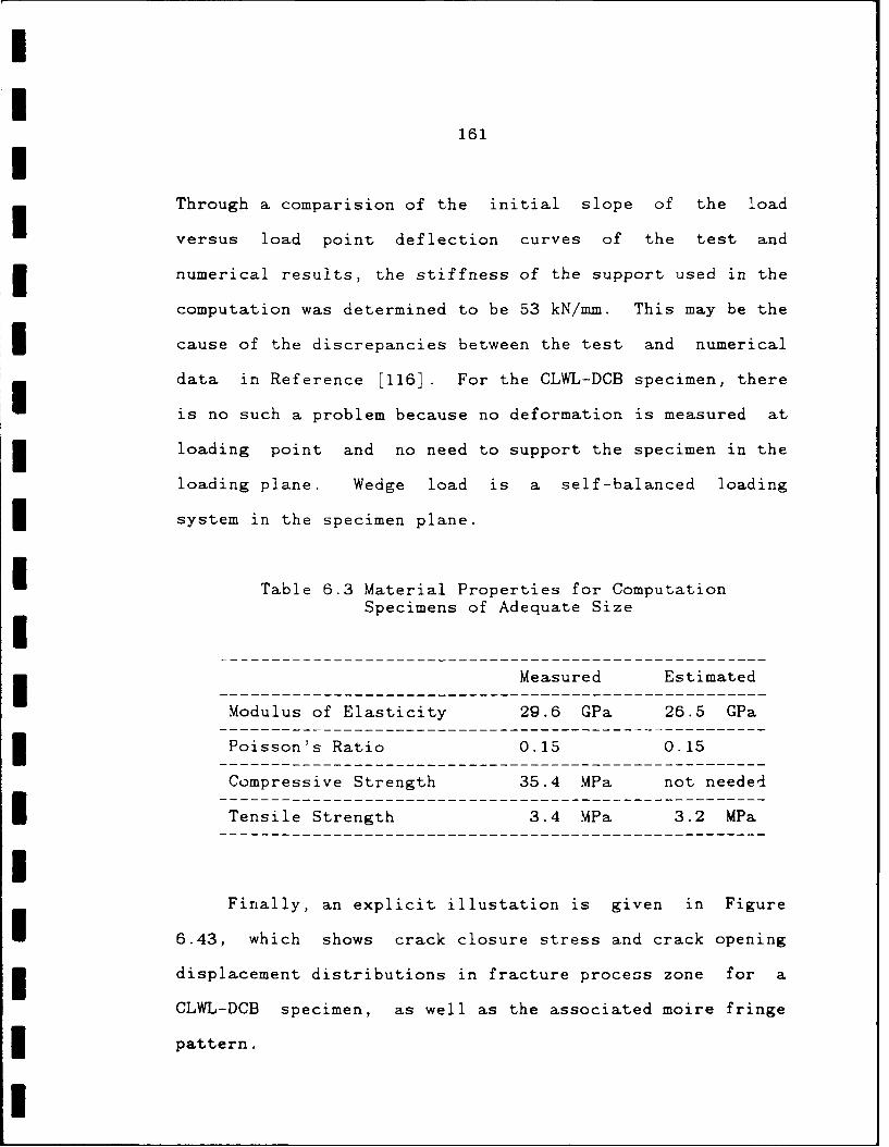
161
Through a comparision of the initial slope of the load
versus load point deflection curves of the test and
numerical results, the stiffness of the support used in the
computation was determined to be 53 kN/mm. This may be the
cause of the discrepancies between the test and numerical
data in Reference [116]. For the CLWL-DCB specimen, there
is no such a problem because no deformation is measured at
loading point and no need to support the specimen in the
loading plane. Wedge load is a self-balanced loading
system in the specimen plane.
I Table 6.3 Material Properties for ComputationSpecimens of Adequate Size
I Measured Estimated
Modulus of Elasticity 29.6 GPa 26.5 GPa
Poisson's Ratio 0.15 0.15
Compressive Strength 35.4 MPa not needed
I Tensile Strength 3.4 MPa 3.2 MPa
IFinally, an explicit illustation is given in Figure
6.43, which shows crack closure stress and crack opening
displacement distributions in fracture process zone for a
CLWL-DCB specimen, as well as the associated moire fringe
I pattern.
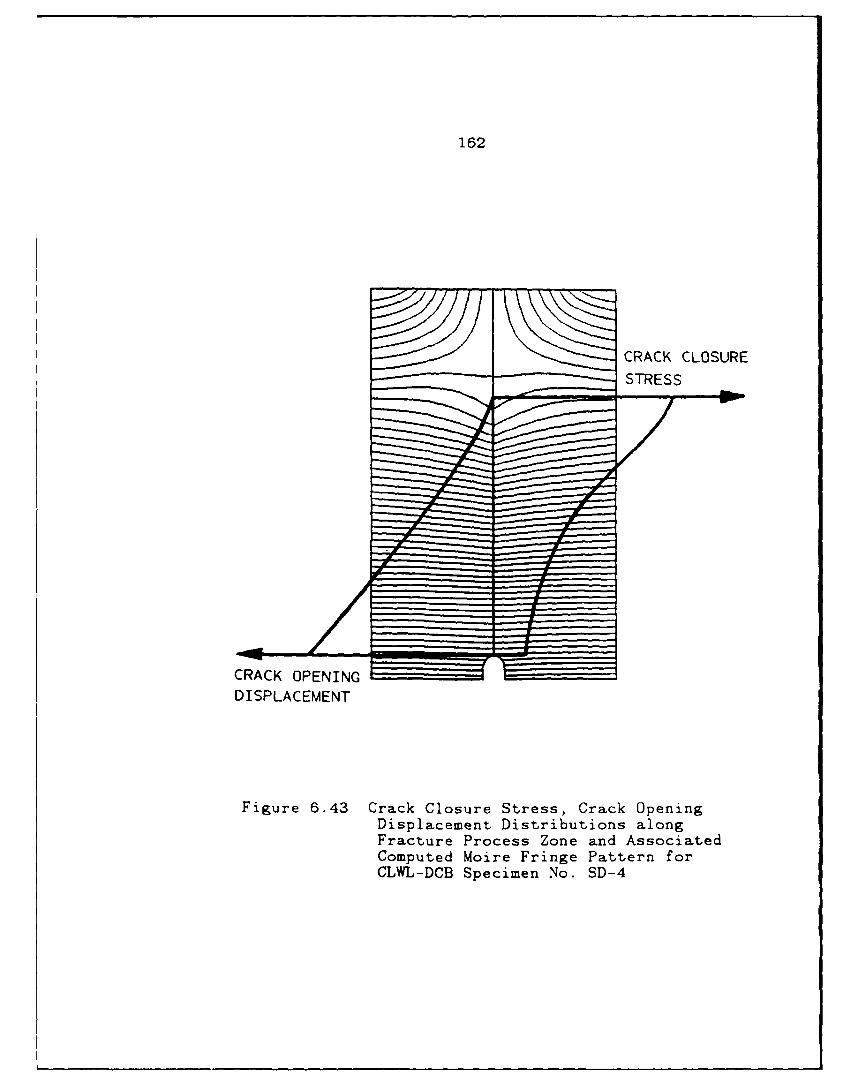
162
CRACK CLOSURE_ STRESS
CRACK OPENING
DISPLACEMENT
Figure 6.43 Crack Closure Stress, Crack OpeningDisplacement Distributions alongFracture Process Zone and AssociatedComputed Moire Fringe Pattern forCLWL-DCB Specimen No. SD-4
CHAPTER SEVEN
DYNAMIC FRACTURE OF CONCRETE SPECIMENS
Dynamic fracture mechanics has not been well developed
even for metals. For concrete, results are even fewer. In
this research area, two types time dependent phenomena and
their combinations are investigated. Dynamic fracture can
be the case of dymamic load with static crack or dynamic
crack with static load or both of them are dynamic. The
subject of this study belongs to the third category.
* In this chapter the fracture process zone model
developed for stable crack growth in concrete was extended
to simulate dynamic crack propagation in concrete members
subjected to impact loading conditions. A dynamic linear
elastic finite element code with build-in function of the
* fracture process zone effect was developed and executed to
predict specimen behaviors and study the strain rate
* effects on fracture of concrete.
I 7.1 Dynamic Fracture Process Zone Model.
7.1.1 General
The commonly observed strain softening effect in
static fracture of concrete tests has also been observed in
concrete dynamic direct tension tests '86], This means that
fracture process zone generally exists in cracked concrete
164
members so that any single parameter model of dynamic
fracture mechanics is neither appropriate. The question is
that if the Dugdale type fracture process zone model
developed for static fracture is still valid for modelling
dynamic fracture of concrete, and if the answer is
positive, what kind of modefications should be made to
represent strain rate effect. In order to answer these
questions, specimens of different geometries and materials
must be tested and multiple identical specimens should be
tested at different loading rates together with dynamic
finite element analysis. Since the dynamic test apparatus
had not been set up at University of Washington when this
work was carried out, test results from Mindess et al.
L88,89] at the University of British Colonbia and from Shah
et al. [91,92] at the Northwestern University were used as
data bases for developing a fracture process zone model.
7.1.2 Formulation Considerations
Although the use of the superposition principle and
Green functions reduces computing time for the simulation
of the static fracture process zone, it does not when the
inertial forces are included for dynamic finite element
computation. The reason is that inertial forces are
applied on every nodal point so that too many fundamental
solutions must be computed and saved on the computer.
165
Hence, the formulation based on the superposition
principle, described in Chapter 5, was not used for the
dynamic finite element computations. Instead, a direct
finite element computation using three-line model was
conducted.
For constructing the dynamic fracture process zone
model, all the assumptions used for static fracture study
in the foregoing chapters are still valid here. The
details of the dynamic finite element implementation are
U given in APPENDIX D and only the essential procedures are
*presented here.
7.2 Preliminary Results
7.2.1 Simulation of Mindess' Impact Tests
The fracture process zone model used in this analysis
3 was derived, through a hybrid experimental-numerical
technique, from the results of laboratory tests of static
I mode I and mixed mode I and II fracture of concrete
3 CLWL-DCB specimens. As shown in Figure 7.1, the variation
in the crack closure stress in fracture process zone can be
3 approximated by three straight lines which intersect at
three critical crack widths. Figure 7.2 shows the
I constitutive model, for the fracture process zone, which
3 relates the crack closure stress and crack opening
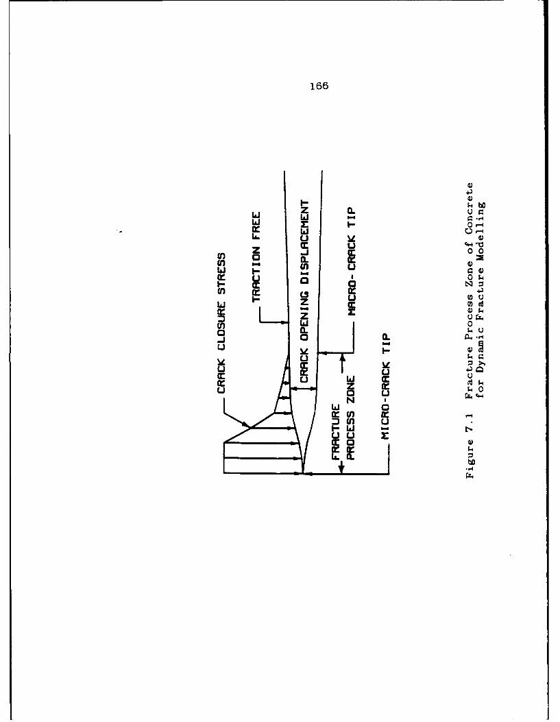
166
z CLLI 0-
T. UZ .j 0 0
m 0
w z
a ia60 0. -
LI 0
It lzu t 4-)
E u u
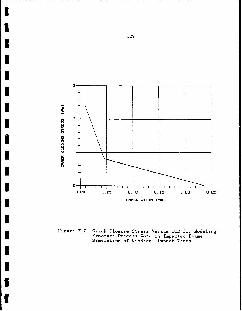
UI
167
I
UUII
U
* z -
30.00 0.05 0.10 0.15 0.20 0.25
3 CRACK WIDTH (nmm)
Figure 7.2 Crack Closure Stress Versus COD for ModelingFracture Process Zone in Impacted Beams.SSimulation of Mindess' Impact Tests
I€Iw
It
168
displacement in the fracture process zone. This
constitutive relation was developed originally for static
loading fracture [9]. Also, it was assumed that dynamic
linear elasticity theory is still valid in the region
outside the fracture process zone.
The fracture process zone model was incorporated into
an implicit dynamic finite element code. The three
segments of the fracture process zone, which satisfy the
crack closure stress versus COD relation shown in
Figure 7.2, are determined through numerical iteration.
That iterative scheme is similar to the
incremental-iterative procedure of elastic-plastic
analysis. It consists of matching, through trial and
error, an assumed variation in crack width along the
postulated fracture process zone with the computed crack
width for the prescribed load history and crack closure
stress distribution.
The fracture criterion is a simple tensile overload
criterion with fracture occuring along the preset crack
path for mode I crack propagation when the maximum average
tensile stress in the assumed controlled volume, that is
the maximum aggregate size, of the crack tip element
reaches the prescribed tensile strength. In Figure 7.3,
the broken and solid lines indicate the position of the
crack prior to and after its advancement, respectively, and
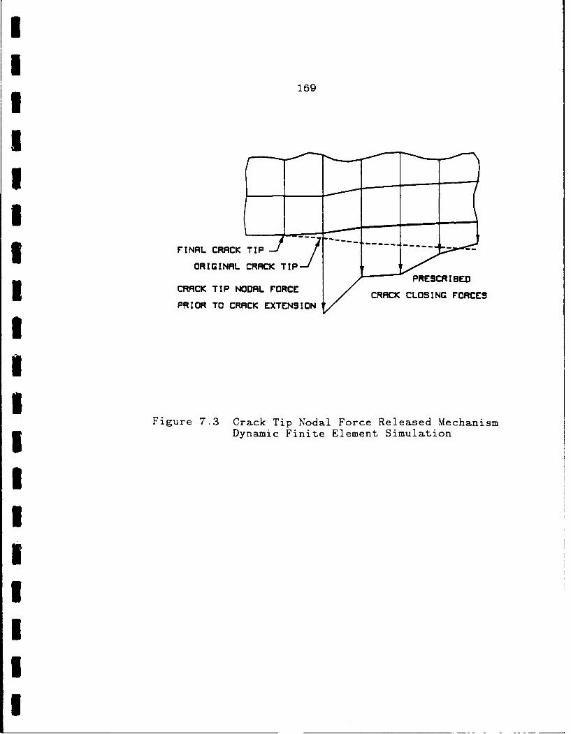
II
169
I
IIFINAL CRACK TIP ... '
ORIGINAL CRACK TIP PRESCRIBED
CRACK TIP NODAL FORCE CRACK CLOSING FORCES
PRIOR TO CRACK EXTENSION
I
Figure 7.3 Crack Tip Nodal Force Released MechanismDynamic Finite Element Simulation
i
IIIii
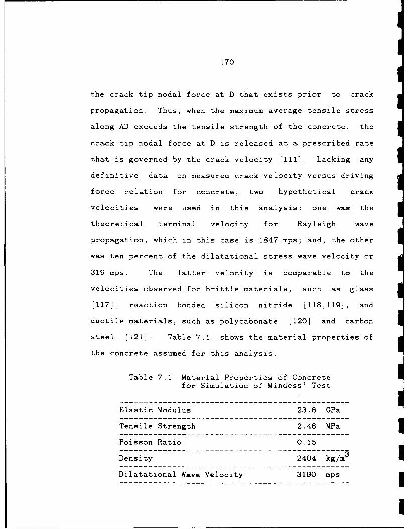
170
the crack tip nodal force at D that exists prior to crack
propagation. Thus, when the maximum average tensile stress
along AD exceeds the tensile strength of the concrete, the
crack tip nodal force at D is released at a prescribed rate
that is governed by the crack velocity [Ill]. Lacking any
definitive data on measured crack velocity versus driving
force relation for concrete, two hypothetical crack
velocities were used in this analysis: one was the
theoretical terminal velocity for Rayleigh wave
propagation, which in this case is 1847 mps; and, the other
was ten percent of the dilatational stress wave velocity or
319 mps. The latter velocity is comparable to the
velocities observed for brittle materials, such as glass
L117], reaction bonded silicon nitride [118,119], and
ductile materials, such as polycabonate [120] and carbon
steel '121] . Table 7.1 shows the material properties of
the concrete assumed for this analysis.
Table 7.1 Material Properties of Concretefor Simulation of Mindess' Test
Elastic Modulus 23.6 GPa
Tensile Strength 2.46 MPa
Poisson Ratio 0.15
Density 2404 kg/m3
Dilatational Wave Velocity 3190 mps
-------------------------------------

I1
171UImpact Test Specimen No. I
Figure 7.4 shows the proportions, l)ading, and
3 instrumentation for a plain concrete beam. That beam was
impacted by a falling hammer at an impact velocity of about
S3 mps -88]. Figure 7.5 shows the load history as measured
at the hammer [88]. Figure 7.6 shows the finite element
mesh used in the analysis. Figures 7.7 and 7.8 show the
computed lengths for crack extension with time, with and
without the fracture process zone, for assumed
3 instantaneous crack velocities of 1847 mps and 319 mps,
respectively. The computed response is indicated by
stepwise broken lines. The computation was terminated at
if the last element in the crack path, and the elapsed time
from initial impact to complete failure of the beam had to
3 be estimated by fitting a curve through those discontinuous
run-arrest crack paths. The average crack velocities
obtained from the computation with the fracture process
3 zone are in good agreement with that of the test results.
On the otherhand, the average crack velocities obtained
3 from the computation without the fracture process zone are
too high compared to the test result. These results
suggest that energy is dissipated within fracture process
3 zone and in turn retards crack propagation even under
dynamic loading. It should also be noted that the computed
Stime to failure is relatively insensitive for the two
tieIo h
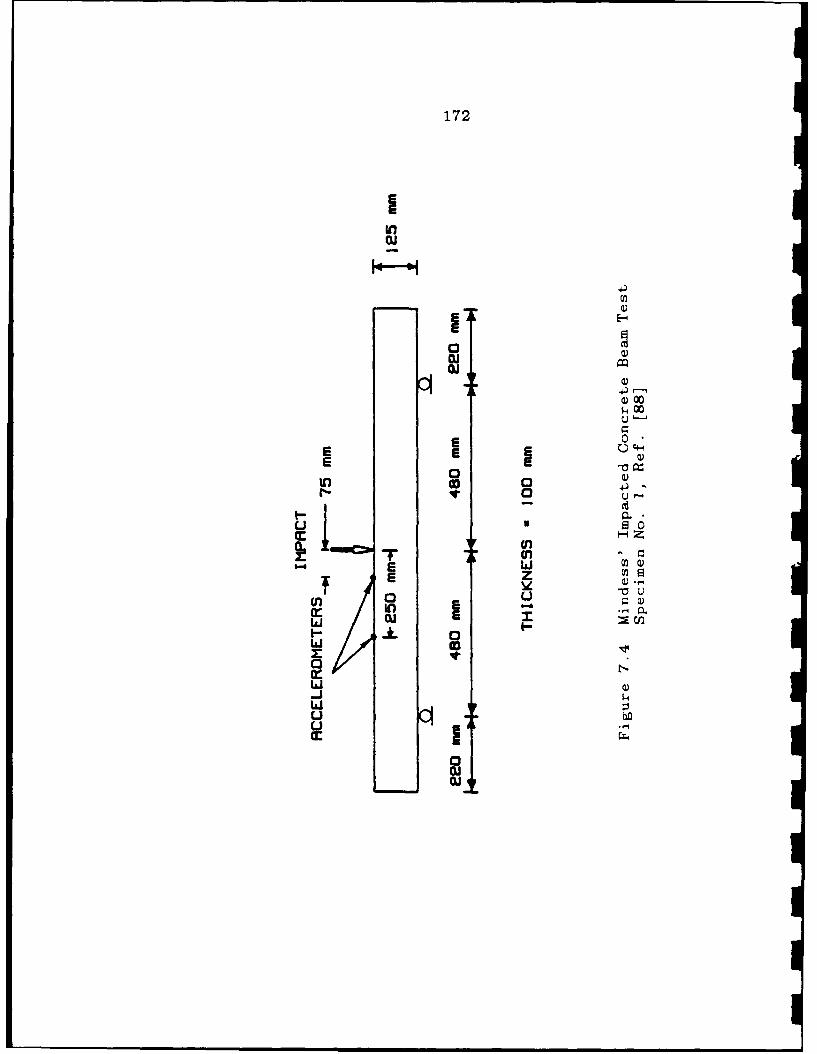
172
in
00o00
QC
E 0*
0 U
1*~ ~ 00r
z~ 7 U -
cn 0 u 0
W) r. Q0
0wd0
w~bf
u ci buI
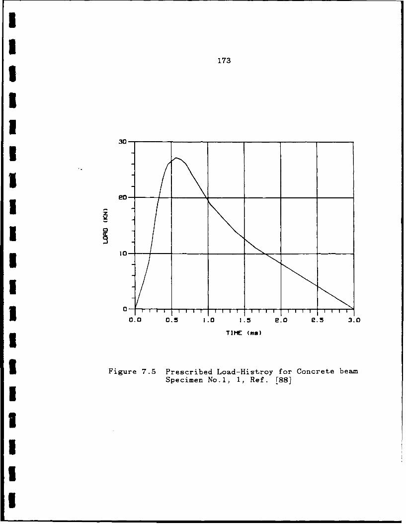
II
173II
30II 20-
3 a0.0 0.5 1.0 1-.5 r.0 e.5 3.0
TIME (ms)
I Figure 7.5 Prescribed Load-Histroy for Concrete beamSpecimen No.1, 1, Ref. [88]U
IIII
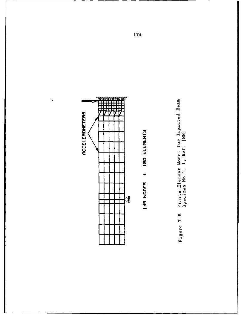
174
(n v v
Li z 0Lhi 0
Li r 0
r-.4 Q
oQ -~
60
+)(n UUl
44 )
.1*4

I
175
Ii e5
-5
Iz t COMI'PUJTED F ITTED
v 5-
e5 - WITOU PUTRRCTURE
[¢PROCESS ZONE ----------
0 - I I I
0.0 0.5 1.0 1.5 2.0
TI ME (ms)
Figure 7.7 Computed Crack Length Versus Time
Specimen No. 1, Ref. [88]Assumed Crack Velocity 1847 mps
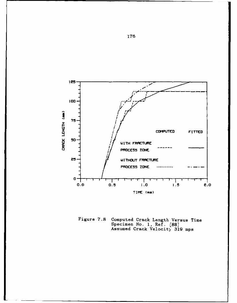
176
125-
I r
751
COMPUTED FITTED
WUI TH FRACTURE _
PROCESS ZONE
e5 U I THOUT FRRCTURE
PROCESS ZONE - ---------
0.0 0.5 1.0 1.5 e.0
TIME (ms)
Figure 7.8 Computed Crack Length Versus TimeSpecimen No. 1, Ref. [88]Assumed Crack Velocit) 319 mps
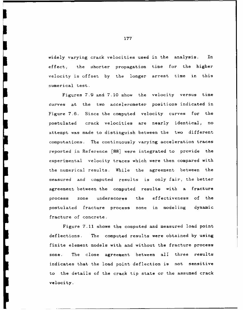
I
177
widely varying crack velocities used in the analysis. In
effect, the shorter propagation time for the higher
velocity is offset by the longer arrest time in this
numerical test.
Figures 7.9 and 7.10 show the velocity versus time
curves at the two accelerometer positions indicated in
Figure 7.6. Since the computed velocity curves for the
postulated crack velocities are nearly identical, no
attempt was made to distinguish between the two different
computations. The continuously varying acceleration traces
reported in Reference [88] were integrated to provide the
experimental velocity traces which were then compared with
the numerical results. While the agreement between the
measured and computed results is only fair, the better
agreement between the computed results with a fracture
process zone underscores the effectiveness of the
postulated fracture process zone in modeling dynamic
fracture of concrete.
Figure 7.11 shows the computed and measured load point
deflections. The computed results were obtained by using
finite element models with and without the fracture process
zone. The close agreement between all three results
indicates that the load point deflection is not sensitive
to the details of the crack tip state or the assumed crack
velocity.
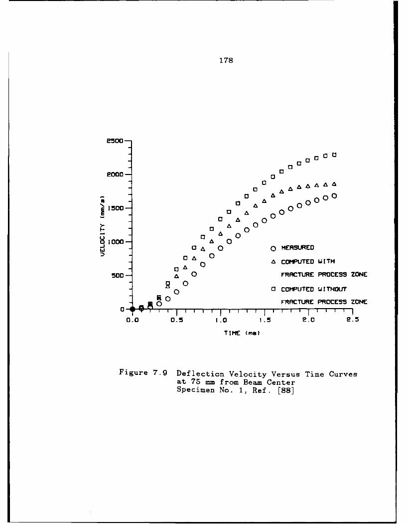
178
2500
0000 O0 0
0
o 0
0 0
500- 0 0RCUEPOESZN
0 0
u0F U 0a 1000- A 0.j -0 4 0 0 MEASUJREDw
0-00 C3 COMPUTED W ITHOUT
S0 FRCTURE PROESS ZONE
0.0 0.5 1.0 1.5 2.0 2.5
TIME (me)
Figure 7.9 Deflection Velocity Versus Time Curvesat 75 mm from Beam CenterSpecimen No. 1, Ref. [88]

179
II
E3 E3 AA Aa
0 A A100 ° o 0 0
10 0-J3 0A
0 0 0 MEASURED
00I 0 COMPUTED (JITh00
0 COMPUTED WITHOUAoZ 0 FRRC'URE. PROCESS ZONE
I 0 oCOMPUTED W ITHOUT
FRACTURE PROCESS ZONE
0.0 0.5 1.0 1.5 .0 e.5
TIME (ms)
I Figure 7.10 Deflection Velocity Versus Time Curvesat 250 mm from Beam CenterSpecimen No. 1, Ref. [88]
I
II
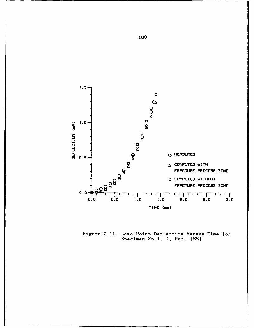
180
0
A
i.j
0.5 2COMPUTED WIT H1
FRRCTURE PROCESS ZONE
00 0 COMPUTED WITHOUT
a 0FRRCTURE PROCESS ZONE
0.0 0.5 1.0 1.5 2.0 e.5 3.0
TIME (me)
Figure 7.11 Load Point Deflection Versus Time forSpecimen No.1, 1, Ref. [88]
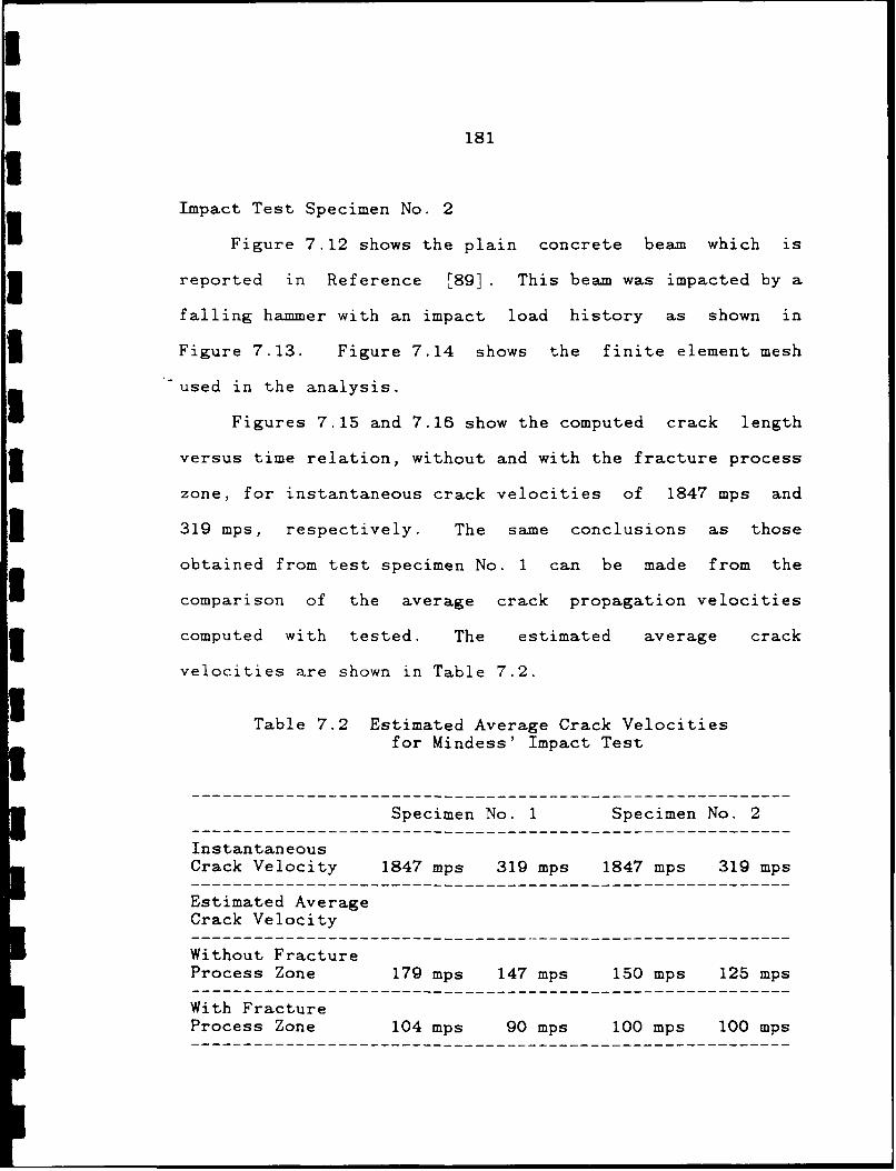
I181
Impact Test Specimen No. 2
Figure 7.12 shows the plain concrete beam which is
reported in Reference [8 9 ]. This beam was impacted by a
falling hammer with an impact load history as shown in
Figure 7.13. Figure 7.14 shows the finite element mesh
used in the analysis.
Figures 7.15 and 7.16 show the computed crack length
3 versus time relation, without and with the fracture process
zone, for instantaneous crack velocities of 1847 mps and
319 mps, respectively. The same conclusions as those
obtained from test specimen No. 1 can be made from the
comparison of the average crack propagation velocities
computed with tested. The estimated average crack
velocities are shown in Table 7.2.
Table 7.2 Estimated Average Crack Velocitiesfor Mindess' Impact Test
Specimen No. 1 Specimen No. 2
InstantaneousCrack Velocity 1847 mps 319 mps 1847 mps 319 mps
Estimated AverageCrack Velocity
Without FractureProcess Zone 179 mps 147 mps 150 mps 125 mps
With FractureProcess Zone 104 mps 90 mps 100 mps 100 mps
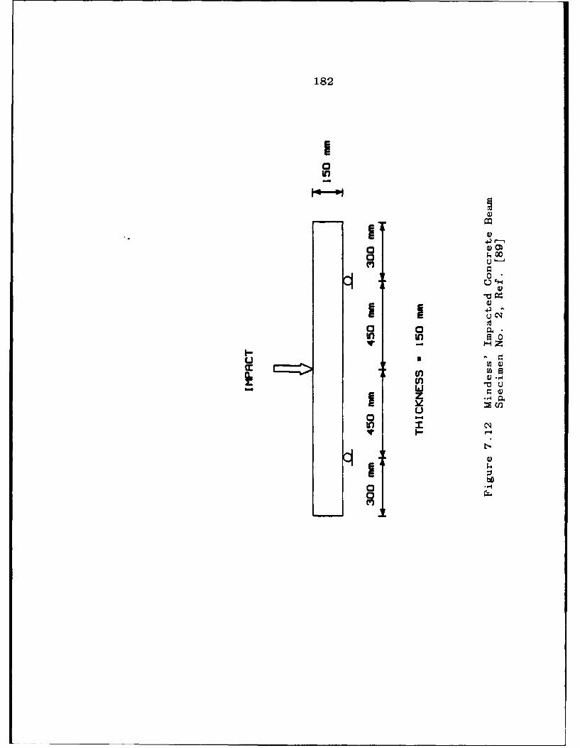
182
I0In
Q)
0*
0)
4-)I C1In in a20
1W. -
I U(I,0 4) -
I a
C-,C
Lo
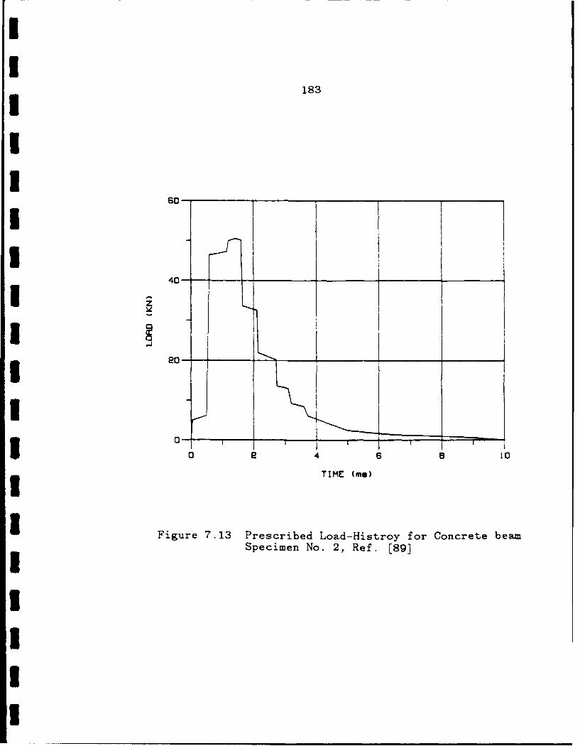
II
183
II
I~60-I
40-
I -z
eo-
0 4 6 a 10
TIME (me)
I Figure 7.13 Prescribed Load-Histroy for Concrete beamSpecimen No. 2, Ref. [89]
II
I[
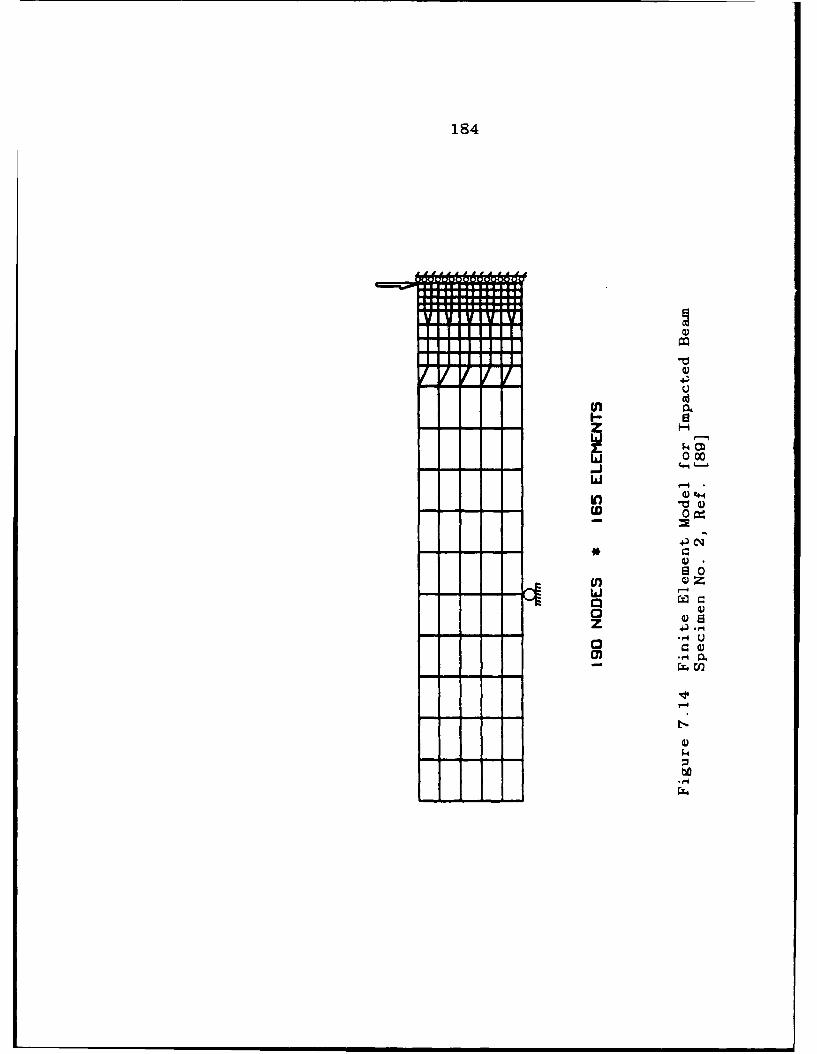
184
(I)d- lad
-- z
3 000
Q) z
Cm,
z .C
bO-x4
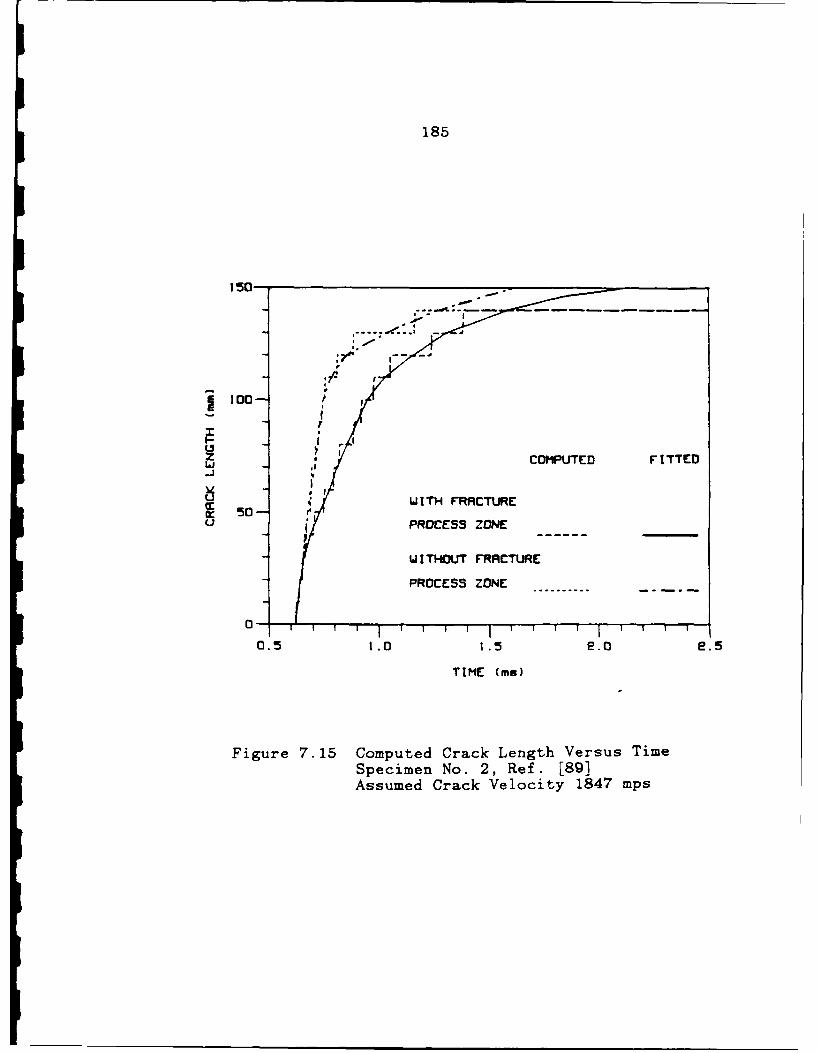
185
II150,._ _- = _
50 -
I OMU'EDFITTED
I WITH FRRCTURE50-
u PROCESS ZONE
WITHOUT FRACTURE
PROCESS ZONE
0-0.5 1.0 1.5 e.o e.5
TIME (me)
Figure 7.15 Computed Crack Length Versus TimeSpecimen No. 2, Ref. [89]Assumed Crack Velocity 1847 mps
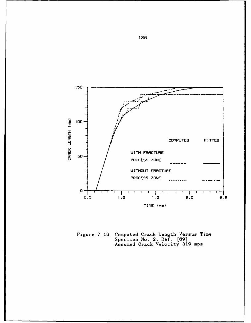
186
150-
Z COMPUTED FITTED
U WI !TH FRRCTUREw 50- /U/ PROCESS ZONE
WITHUTFRR9CTURE
~PROCESS ZONE
0 1o T 1-
0.5 1.0 1.5 e.0 e.5
TIME (me)
Figure 7.16 Computed Crack Length Versus TimeSpecimen No. 2, Ref. [89]Assumed Crack Velocity 319 mps
187
3 An advantage of the finite element analysis is that
one numerical experiment will provide a multitude of
3 numerical data. One such data is the energy partition
during fracture. Figures 7.17 and 7.18 show the variations
I in the kinetic, strain and fracture energies, with time.
The sum of these three energies, at any instant, was within
one percent of the accumulated external work, which was
3 computed independently. This agreement which differs with
the results of Reference [88], provided a consistency check
I on the numerical procedure. Unlike other fracture
specimens '1221, Figures 7.17 and 7.18 show that the
kinetic energy dominates and is the primary energy sink for
3absorbing the input work for these impacted concrete
specimens.
7.3 Refined ResultsI7.3.1 Simulation of Shah's Impact TestsI
This simulation also used three-line model. For
3 dynamic analysis, the three critical crack opening
displacements wl, w2 and w3 in Figure 7.19, were assumed to
be strain rate invariant and only the dynamic tensile
3 strength was assumed to be strain rate dependent. That
dependency was assumed to vary at the same rate as the
3 observed variations in the total work to fracture in the

188
EXTERNAL WORK40-
30-1 " KINETIC ENERGY
Z 20- F""
0.0 0.5 1.0 1.5 e.o e.5 3.0
TIME (ms)
Figure 7.17 Energy Partition for Impacted BeamSpecimen No. 1, Ref. [88]Assumed Crack Velocity 1847 mps
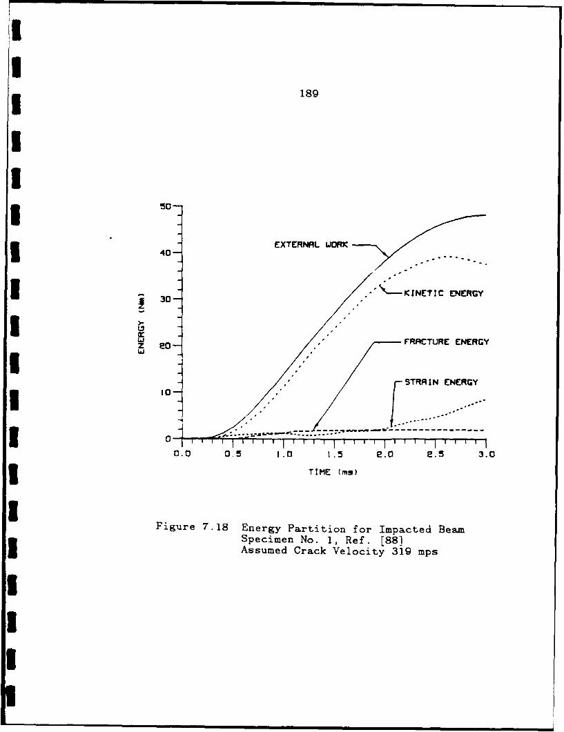
189
I
3 EXTERNAL WORK40-
30- ."-KINETIC ENERGY
I 3-
STRAIN ENERI I0-.O' '
3 -- -- ------.. .. ..I t
1 1111 '' i' I l ii I I I I
0.0 0.5 1.0 1.5 e.0 2.5 3.03 TIME (ms)
Figure 7.18 Energy Partition for Impacted BeamSpecimen No. 1, Ref. [88]Assumed Crack Velocity 319 mps
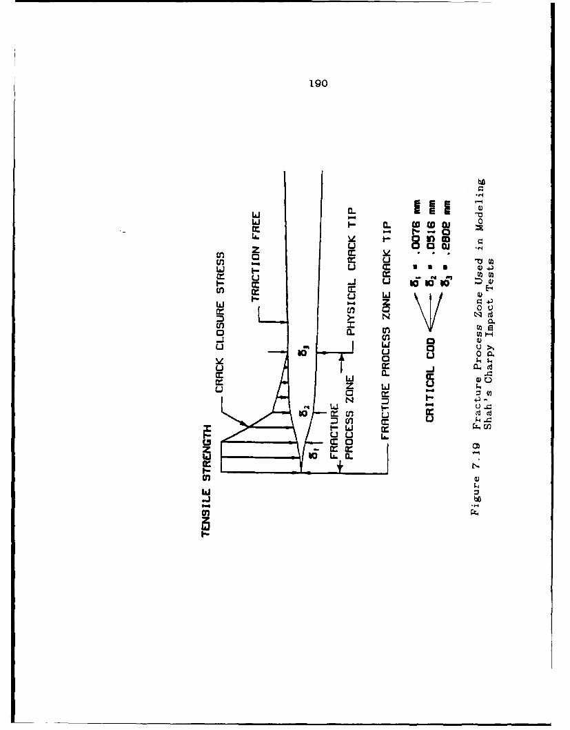
190
(U
I- M~0 0i 00
(n c .a, - ~
LI I- uI ~ unw T
C, 0 0tN \I
0~~ 0.U,
a..
m L)uZ Li La :2 W
N 4--to4 Li -(n um d-
I---m
m
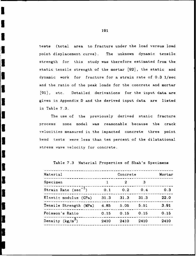
191
tests (total area to fracture under the load versus load
point displacement curve). The unknown dynamic tensile
3 strength for this study was therefore estimated from the
static tensile strength of the mortar [92], the static and
I dynamic work for fracture for a strain rate of 0.3 I/sec
and the ratio of the peak loads for the concrete and mortar
[91], etc. Detailed derivations for the input data are
3 given in Appendix D and the derived input data are listed
in Table 7.3.
3 The use of the previously derived static fracture
process zone model was reasonable because the crack
velocities measured in the impacted concrete three point
3 bend tests were less than ten percent of the dilatational
stress wave velocity for concrete.ITable 7.3 Material Properties of Shah's Specimens
Material Concrete Mortar
Specimen 1 2 3
Strain Rate (sec -I ) 0.1 0.2 0.4 0.3
Elastic modulus (GPa) 31.3 31.3 31.3 22.0
3 Tensile Strength (MPa) 4.85 5.05 5.51 3.91
Poisson's Ratio 0.15 0.15 0.15 0.15
Density (kg/m3) 2410 2410 2410 2410
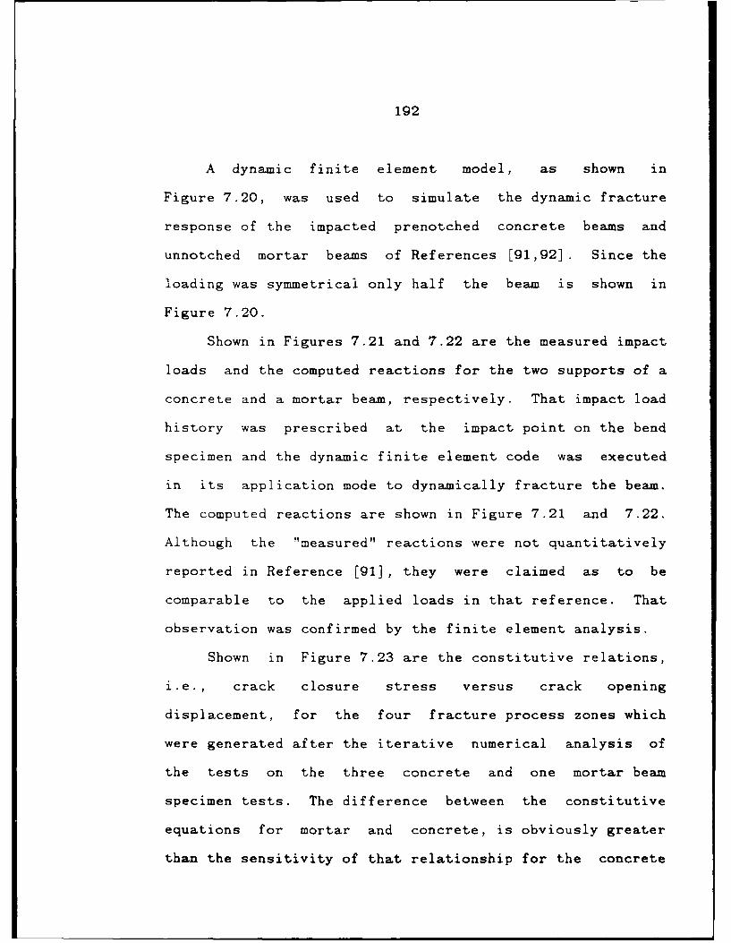
192
A dynamic finite element model, as shown in
Figure 7.20, was used to simulate the dynamic fracture
response of the impacted prenotched concrete beams and
unnotched mortar beams of References [91,92]. Since the
loading was symmetrical only half the beam is shown in
Figure 7.20.
Shown in Figures 7.21 and 7.22 are the measured impact
loads and the computed reactions for the two supports of a
concrete and a mortar beam, respectively. That impact load
history was prescribed at the impact point on the bend
specimen and the dynamic finite element code was executed
in its application mode to dynamically fracture the beam.
The computed reactions are shown in Figure 7.21 and 7.22.
Although the "measured" reactions were not quantitatively
reported in Reference [91], they were claimed as to be
comparable to the applied loads in that reference. That
observation was confirmed by the finite element analysis.
Shown in Figure 7.23 are the constitutive relations,
i.e., crack closure stress versus crack opening
displacement, for the four fracture process zones which
were generated after the iterative numerical analysis of
the tests on the three concrete and one mortar beam
specimen tests. The difference between the constitutive
equations for mortar and concrete, is obviously greater
than the sensitivity of that relationship for the concrete
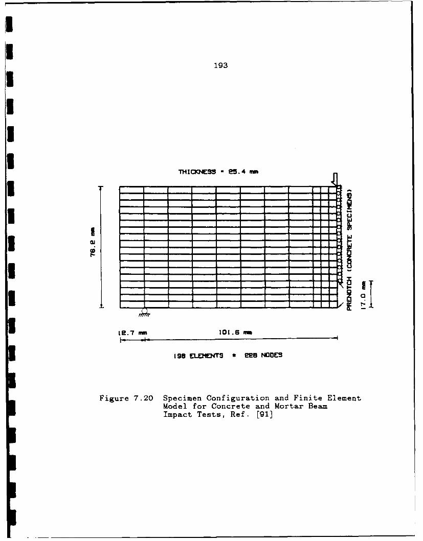
II
193I
IIi THICKNESS e5.4 -m
ie1.'7 mm 101.6 MM
198 ELE[MENTS * e8 NqODE'S
Figure 7.20 Specimen Configuration and Finite ElementModel for Concrete and Mortar BeamImpact Tests, Ref. [91]
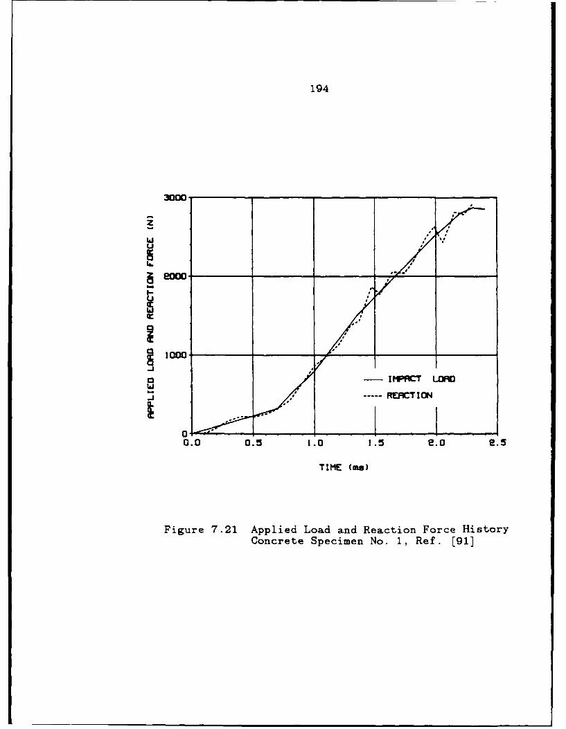
194
I./.
w -
i ..... f .RUCT ION
0.0 0.5 1 . 1.5 e.o e.5
TIME (me)
Figure 7.21 Applied Load and Reaction Force HistoryConcrete Specimen No. 1, Ref. [91]

195
5 000-
e z
14000.
I _ _ I° _ _ .. " "
as
10
0.0 O.e 0.4 0,6 0.8 1.0
TIME (me)
Figure 7.22 Applied Load and Reaction Force HistoryMortar Specimen, Ref. [92]
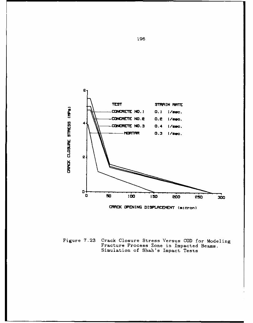
196
TEST STRRIN RRrE
COCETE NO. 1 0. 1 1i/sec.
coNCRtETE No.e 0.2 i/secCONCRETE NO.3 0.4 1/sec.
" MORTRR 0. 3 1/8sc.
U e.
0 50 100 150 800 250 300
CROCK OPENING DISPLCEMENT (micron)
Figure 7.23 Crack Closure Stress Versus COD for ModelingFracture Process Zone in Impacted Beams.Simulation of Shah's Impact Tests

197
beam test to strain rate variations between 0.1 and 0.4
1/sec.
Although not apparent from Figure 7.23, the
computations also showed that the process zone length
decreased with increasing strain rate. A similar trend was
observed experimentally by Shah et al. [91]. A higher
strain rate increases the dynamic tensile strength.
However, the accompanying decrease in the fracture process
zone length offsets that increase, the total dissipated
fracture energy, were nearly invariant for the strain rate
variations examined in this study.
Shown in Figures 7.24 and 7.25 are typical computed
and measured crack extension histories for the concrete and
mortar beams. Knowing that the stair shape of the computed
results is due to the discrepancy of the numerical
analysis, only fitted curves are presented in these
figures. The crack extension histories were measured,
using a KRAK-GAGE.- That gage exhibited some ductility
and thus in Figure 7.24 there is a finite time delay of
about 1 millisecond between the passage of the crack tip as
computed, and the strains as recorded. The slopes of the
computed and measured crack extension histories are,
* TTI Division, Hartran Corporation, FL.
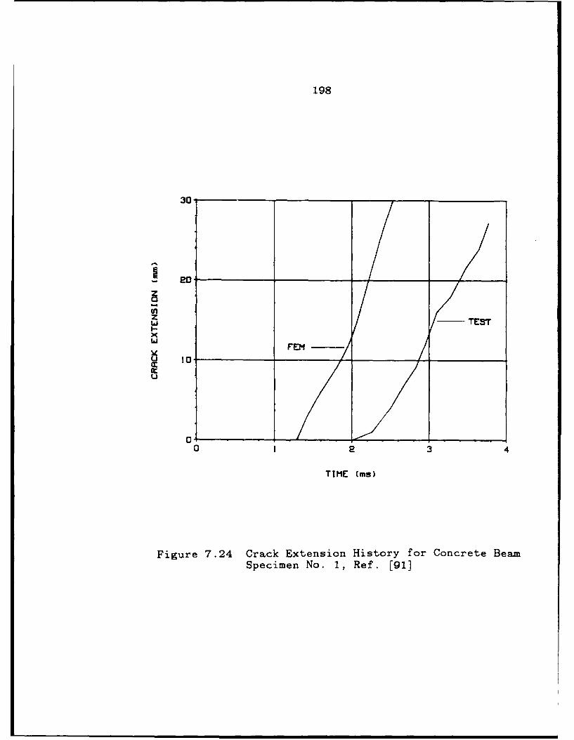
198
30,
zZ TEST
X
U 0
0 I 3 4
TIME (ms)
Figure 7.24 Crack Extension History for Concrete BeamSpecimen No. 1, Ref. [91]
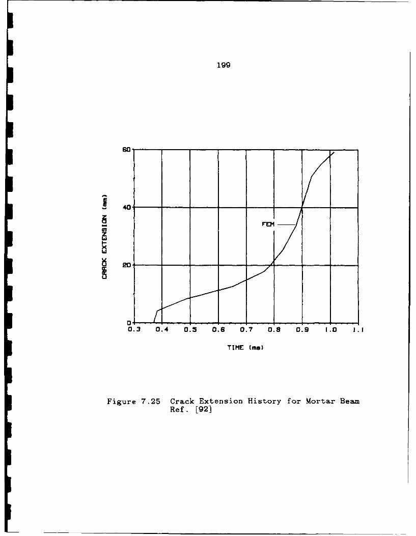
199
40-
0.3 0.4 0.5 0.6 0.7 0.8 0.9 1.0 1.1
TIME (ma)
Figure 7.25 Crack Extension History for Mortar BeamRef. [92]
200
however, in good agreement with each other and indicate
that computed and measured crack velocities are in
agreement despite the time lag in the KRAK-GAGE responses.
Figures 7.26 and 7.27 show the measured and computed
strain histories for the concrete and mortar beams,
respectively. Strains were measured at the notch tip in
the concrete beam and on the extreme tension fiber at the
quarter length of the span for the mortar beam. There is
reasonable agreement between the computed and measured
strains.
Figures 7.28 and 7.29 show the computed deflection
histories for the load point of the three concrete beams
and the mortar beam, respectively. Also shown in
Figure 7.29 is the measured deflection, which is in good
agreement with its computed conterpart, for the mortar
beam. The slope of that curve represents the specimen's
velocity at the impact point. For the mortar beam the
measured and computed specimen velocities for that point
were the same and both were about 100 mm/s. That value is
much less than the measured tup velocity of 2405 mm/s [92]
just prior to impact. The inertia of the beam, plus the
damping effect of the rubber pad provided at the impact
point, were probable causes for this low specimen velocity.
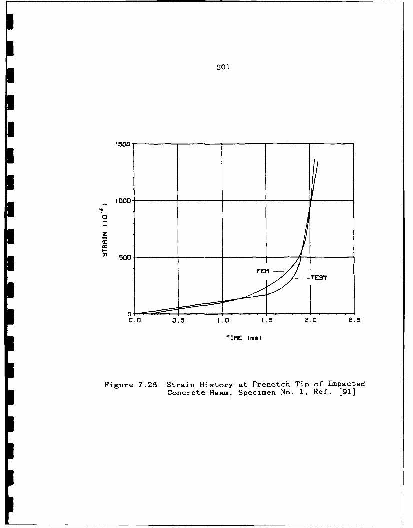
201
1000.0
z
-in 500
0.0 0.5 ! .0 1 .5 e.0 e.5
TIME (ma)
Figure 7.26 Strain History at Prenotch Tip of ImpactedConcrete Beam, Specimen No. 1, Ref. [91]

202
e- .
150-
/
// \\
oo /
100 -
Im.
50 1
0.0 0.2 0.4 0.5 0.8 1.0 1.2 1.4
TIME (me)
Figure 7.27 Strain History at Quarter-Span of ImpactedMortar Beam, Ref. [92]
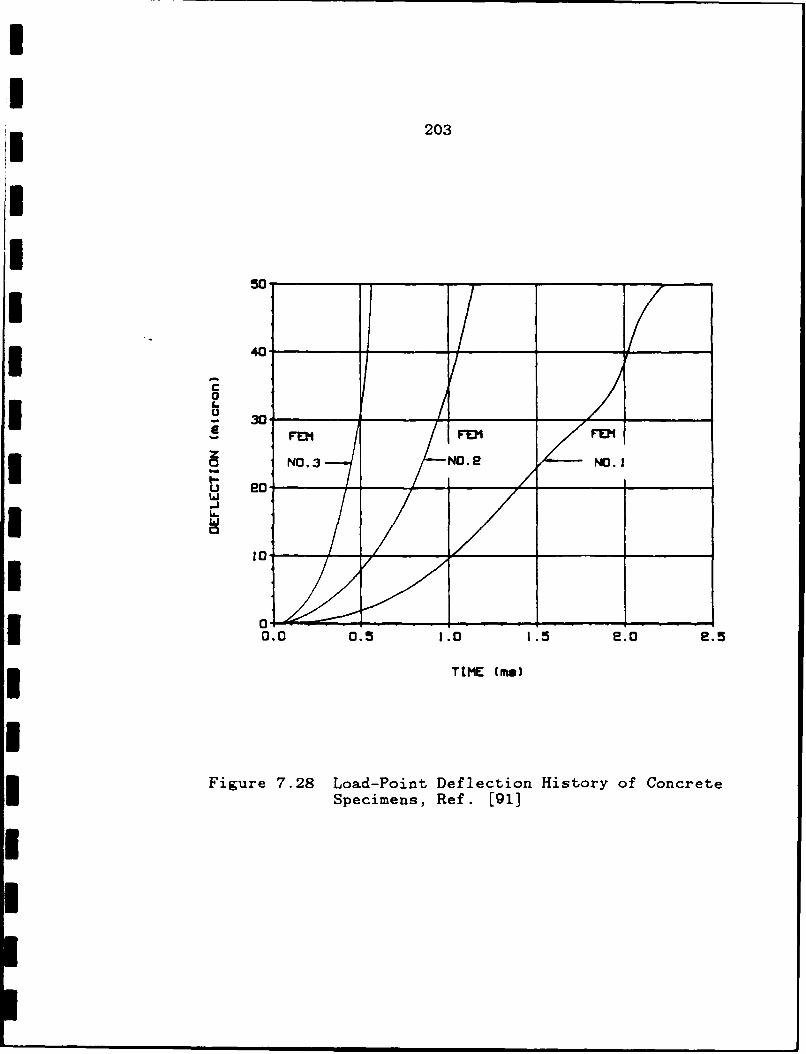
203
50
- 40
U
I- 0E - / E E E6.
w 1 , SI
0 .
0.0 0.5 1.0 1.5 e.O e.5
TIME (me)
Figure 7.28 Load-Point Deflection History of ConcreteSpecimens, Ref. [91]
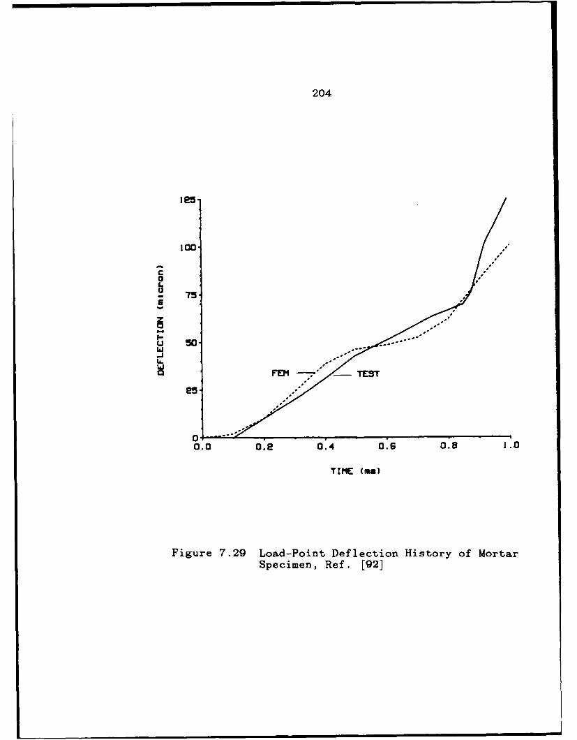
204
oo
75
U 50
w-jIA.
25
00.0 0.e 0.4 0.6 0.8 1.0
TIME (ma)
Figure 7.29 Load-Point Deflection History of MortarSpecimen, Ref. [92]
205
Shown in Figures 7.30 and 7.31 are the energy
partitions for the concrete and mortar beams, respectively.
The relatively small amount of kinetic energy in both
specimens indicates that little of the impact energy was
dissipated to overcome inertial resistance.
Figure 7.32 shows the variations in the dynamic
fracture energy dissipation rate with crack extension. The
rate is shown with respect to unit crack extension. Thus,
those curves represent the dynamic counterpart of crack
*I growth resistance curves in terms of fracture energy
dissipation rate. The strain rate dependence of these
resistance areas is apparent from Figure 7.32. Values
increase with both increasing crack extension and
increasing strain rate.
Figure 7.33 shows the dynamic fracture energy
dissipation rate, with respect to unit crack extension,
versus crack velocity for the concrete beams. This figure
is equivalent to the dynamic fracture toughness versus
crack velocity relationship for metallic and polymeric
dynamic fracture specimens [123]. Typically, those
relationships exhibit a gamma shape. While the same gamma
shape is preserved for the concrete specimens, there is
also a pronounced strain rate effect. Thus a unique
dynamic fracture energy dissipation rate versus crack
velocity relation obviously does not exist for concrete or
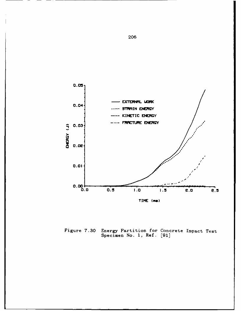
206
0.05.
-EXTERIRL WOWC0.04 STRRIN ENERGY
KINETIC ENERGY
; 0.03,
0.01
-
0.00 -- - " -- -0.0 0.5 1.0 15 e.o e.5
TIME (ms)
Figure 7.30 Energy Partition for Concrete Impact TestSpecimen No. 1, Ref. [91]
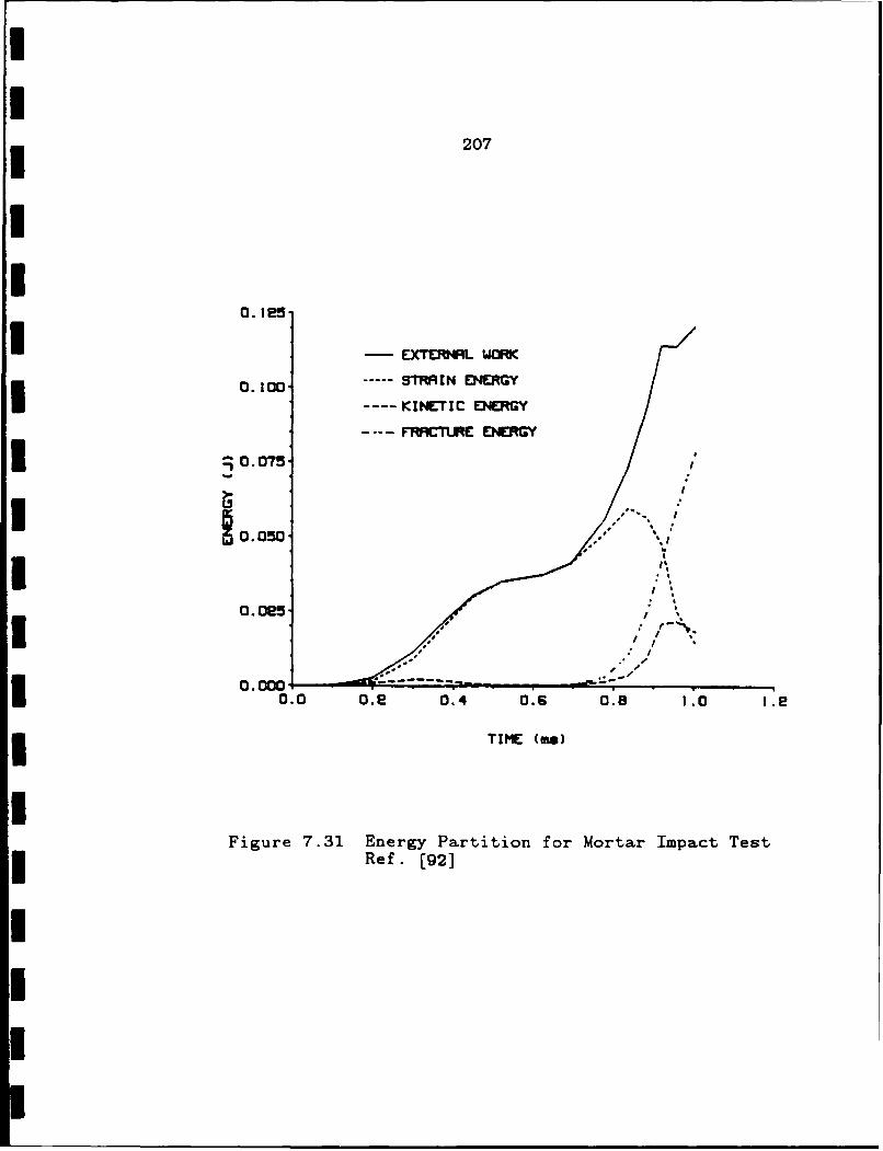
207
U
S-.EXTERNAL WO0.100 - STRAIN ENERGY
--- KINETIC ENERGY- VRFC'TLRE EIEGY
1 0.075
. 050I,
II
0.025.'
0.000 . -
0.0 0.9 0.4 0.6 0.8 1.0 1.2
TIME (me)
Figure 7.31 Energy Partition for Mortar Impact TestRef. [92]
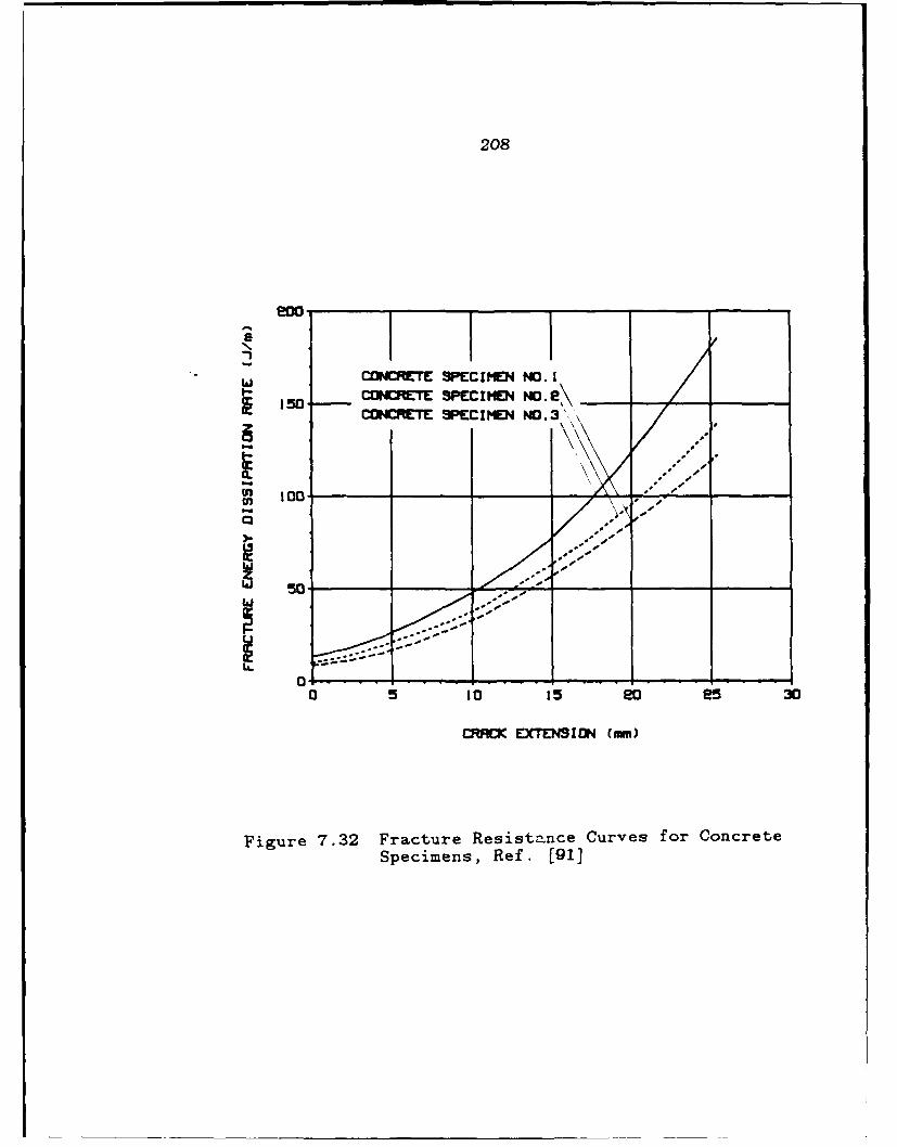
208
CONCRETE SPECIMN NO.ICONCRETE spECIND No. e\-CONCRETE SPECIIEN NO.3
5 00
Specimens, Ref. [91]
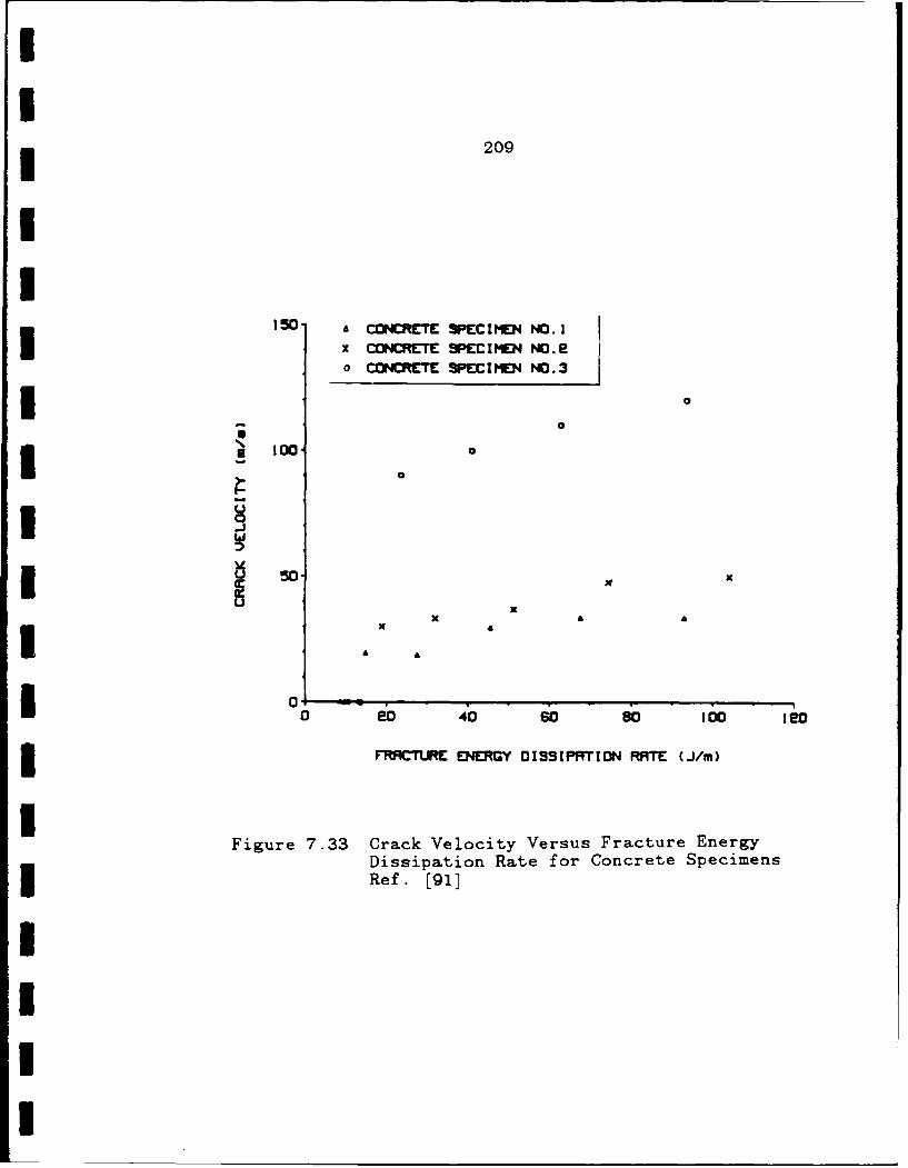
II
209
II
150 ACONCRETE SPECIMEN NO.1
x CONCRETE SPECIMEN NO.2o CONCRETE SPECI MEN NO.3I
I 0
IS
ERf 100.]
U
0
Ix
x I
£FC R ENRG DISSIPRTION (JM /m)
Figure 7.33 Crack Velocity Versus Fracture EnergyDissipation Rate for Concrete SpecimensRef. [91]
210
mortar.
Thus, a theoretical dynamic crack propagation model
for concrete fracture under impact loading has being
constructed. The preliminary results obtained to date show
that the combination of the fracture process zone model
with elasto-dynamic transient finite element analysis is an
appropriate approach for analyzing dynamic fracture of
concrete.

II
5 CHAPTER EIGHT
SUMMARY
1 In this dissertation a systematic study of fracture
mechanics applied to concrete materials is reported. The
prime objective of this study was to define the law
governing tensile failure of concrete under either static
or dynamic conditions. The developments reported here
3 involve new concepts, new test techniques, and new
numerical methods. The significant contributions resulting
3 from this study are summarized in this chapter.
I (1) The essential reasons for differences in the
mathematical models necessary to describe fracture in
3 concrete and fracture in metallic and polymeric materials
have been explained. The large size for the fracture
process zone in concrete means single parameter
3 mathematical models can never effectively characterize that
zone. Also, due to the large resultant strain softening
3 effects, the implications of the whole fracture process
rather than those associated with the fracture point must
be considered. In concrete the fracture point is only the
3 starting point for the fracture process. The final point
in the fracture process is not reached until there is
3 complete material separation and the remaining strength is
zero. This concept explains why traditional fracture
I

212
mechanics concepts cannot be used directly for fracture
analysis of concrete and has indicated the nature of the
model that must be developed for concrete and similar
materials.
(2) Experimental procedures have been developed for
testing concrete fracture specimens. In addition to
conventional experimental techniques, a moire
interferometry technique was developed for studying the
fracture process zone in concrete CLWL-DCB specimens and
three point bend specimens. First, an exploratory white
light moire interferometry test on small specimens revealed
the potential of that method for detecting and measuring
the fracture process zone in a concrete material. Later, a
laser moire interferometry test procedure, with a real
reference grating, was developed which could be used to
observe a fully developed fracture process zone and to
evaluate CODs within that zone in an appropriate sized
specimen. Custom-made diffraction gratings of 600 line/mm
for active or specimen gratings and 1200 line/mm for the
real reference grating were used in these tests.
(3) A numerical procedure was developed for
extracting multiple fracture parameters, that described the
process zone model, and for predicting specimen behavior
such as crack extension, COD in fracture process zone,
stress and displacement field in the specimen, and so on.
213
This numerical procedure included a linear elastic finite
element computation of Green functions and a nonlinear
routine to analyze the fracture process zone based on the
superposition principle. The iteration scheme [49],
developed previously to describe the fracture process zone
behavior, was an indirect nonlinear routine which elied on
physical reasoning and trial and error to obtain results.
In this dissertation that model has been refined and placed
on a mathematical basis. Once that mathematical
formulation was available a direct method for extracting
fracture parameters was developed. This direct method
involved the use of a Newton-Raphson routine, coupled with
a Householder transformation, which effectively optimized
and stabilized the solution of the fracture parameters in
the sense of least squares. A simple smooth curve was used
to describe the functional form of the crack closure stress
versus COD relation. To characterizes that form only three
unknown parameters, including the tensile strength of the
concrete material, need be determined.
(4) Findings on stable crack growth in concrete
specimens can be summarized as the followings:
(a) The development of a fracture process zone or
microcracking zone prior to attainment of the
peak load was clearly observed using moire
214
interferometry. A fully developed fracture
process zone was obtained during the course of
this study.
(b) The fracture process zone width observed in these
tests was about one times the maximum aggregate
size and not three times the maximum aggregate
size as postulated by others [60].
(c) A CLWL-DCB specimen has an inherently rigid
nature that provide stable crack growth. A
simple shop press without any closed loop control
can be used to study the static fracture process
in small scale concrete specimens.
(d) Vibration control is not needed for moire
interferometry testi & when a real reference
grating is used. Thus, the method reported in
this thesis can be used to develop portable
equipment suitable for field testing.
(e) Tensile fracture of concrete has been
successfully modeled using a fracture process
zone characterized )y a unique crack closure
stress versus COD relationship.
(f) The crack closure stress versus COD relation has
been found to be maximum aggregate size dependent
in large specimens. And 25% larger peak load was
obtained for a CLWL-DCB specimen with maximum
215
aggregate size of 6.4 mm than a geometrically
identical specimens with maximum aggregate size
of 9.5 mm.
(g) The smooth curve for the crack closure stress
versus COD relationship derived from the test
data of the CLWL-DCB and three point bend
specimens agreed well with available direct
3 tension results as reported in previous
investigations [12,42,103,104].
3 (h) The three straight line segment model previously
developed was used to check the validity of the
smooth curve model and the direct method. Very
3 good agreement both in the general shape and in
area was obtained.
1 (5) The fracture process zone model developed from
3 static loading results was also used to predict dynamic
fracture of concrete specimens under impact loading
I conditions. The impacted beam tests conducted by Mindess
[88,89] and by Shah [91,92] were used as the data base for
extending that model. An existing dynamic finite element
3 program was modified to alow for incorporation of this
fracture process zone into it. Then that program was
3 executed in its application phase, and the dynamic
responses of the concrete test specimens during theUt
216
fracture process were predicted. Good agreement between
the measured and computed crack velocities, loading point
deflections, strain histories and reactions at supports
were obtained.
(6) Some preliminary strain rate effects for dynamic
fracture of concrete that have been obtained to date are as
follows:
(a) The three critical CODs which represent the
boundaries of the microcracking, transition and
aggregate bridging sub-process zone within the
overall model were strain rate invariant for the
strain rate regime studied.
(b) The dynamic tensile strength of the fracture
process zone is less strain rate dependent than
tensile strengths inferred from the results of
impacted Modulus of Rupture specimens.
(c) The unique gamma curve for dynamic fracture
energy dissipation rate versus crack velocity
that exists for metals and polymers does not
exist for concrete. For concrete that curve
shows considerable strain rate effect.
(d) The experimental observation that the fracture
process zone length decreased with increasing
strain rate was confirmed analytically by dynamic

II
217
Ifinite element modeling.
IIIIII3IUIIIIII
CHAPTER NINE
CONCLUSIONS
The salient conclusions from this investigation are as
follows:
(1) Fracture mechanics method developed for metallic or
polymeric materials can not be applied directly to
concrete and a method, appropriate for concrete, is
developed in this study.
(2) The form of the fracture process zone for concrete and
variations in CODs along that zone can be determined
by the moire interferometry procedures developed in
thi study.
(3) The fracture process zone for concrete has a length
that is dependent of specimen geometry and size and a
width is about one times the maximum aggregate size.
(4) A fracture process zone model that relates crack
closure stress to COD is an excellent one for
predicting the tensile fracture behavior of concrete.
(5) An appropriate direct solution for this fracture
process zone model can be formulated using Green
functions and superposition principles.
(6) A smooth curve representation of the crack closure
stress versus COD relationship is appropriate and a
representation can readily be formulated that the same
219
general shape as the three line segment model
developed in prior University of Washington studies.
3 (7) When this fracture process zone model derived from
test data is used, the behavior for other specimen
3 types and loading conditions can be accurately
predicted using finite element analysis.
(8) The fracture process zone model reported here can be
3 readily extended to predictions of the dynamic
responses of concrete fracture specimens subjected to
* impact load.
(9) The dynamic tensile strength of concrete is less
I strain rate sensitive than the results of Modulus of
3 Rupture beam tests.
(10) Dynamic finite element analysis showed that the length
3 of the fracture process zone decreased as the strain
rate increased.
(11) The CLWL-DCB specimen was found to be an inherently
3 rigid specimen suitable for characterizing stable
crack growth in concrete.
3 (12) Moire interferometry that utilizes a real reference
grating does not require vibration control. The
I method reported here can be used to develop portable
equipment suitable for field testing.
3
CHAPTER TEN
RECOMMENDATIONS
Further research on the following topics is
recommended:
(1) As noted in Chapter 6, the CLWL-DCB specimen and the
three point bend specimen are both essentially bend
specimens. As shown in Figures 6-39 and 6-40, the
normal stress distributions along the crack path for
both specimens are very similar to each other.
Therefore, there is a need to develop a specimen in
which there is a different overall stress state field
in order to check the effect of the overall stress
state on the fracture process zone model.
(2) A direct tension test set-up and test procedure should
be developed. Direct tension test results are the
best data form which a mathematical model can be
derived. Although several results can be found in the
literature, one problem remains unsolved. This
problem can be called "rotational instability" and it
is the result to be expected for non-uniform
strain-softening of the material.
(3) The existance or non-existance of mode II fracture in
concrete should be investigated. If this mode exists
then how to model that type of fracture, as well as
221
mixed mode I and II fractures, should be investigated.
(4) A model for concrete fracture under cyclic loading
conditions should be developed. Because a ,complicated
processes that occur during unloading and reloading no
such model currently exists. The work on ceramic
composites reported here (APPENDIX E), however,
provide a rational basis for developing a model for
3 concrete.
(5) Investigations of the strain rate effects during
dynamic fracture of concrete should be continued.
Tests at different strain rates should be conducted in
order to find strain rate effects. Then, finite
element analysis in its application phase should be
used to study the appropriate form for fracture
process zone model as demonstrated by those results.
(6) Investigations should be made of the dynamic mixed
mode fracture of concrete. A model should be
developed for predicting the crack path for dynamic
crack propagation. Such modeling is likely to be a
very challenging task.
(7) Portable moire interferometry equipment, with a real
reference grating, should be constructed and its
suitability for field testing demonstrated.
(8) An analytical procedure that includes strain hardening
or bulk dissipation effects should be developed. For

222
such analyses the whole region under study becomes
nonlinear, The superposition principle can no longer
be used so that computations become much more
complicated and expensived. However, incorporation of
such effects is needed if actual behavior is to be
realistically modeled.
(9) The fracture process zone model developed here should
be extended to fiber and conventional reinforced
concrete. In the later case, the implications of that
model for predicting bond behavior between concrete
and an embedded steel reinforcing bar should be
examined.
(10) The implications of the model developed here for
failure analysis of real structures should be examined
with a view to improving present design requirements
associated with shear, bond, cracking and minimum
reinforcement ratios. In particular an examination
needs to be made of the extent to which traditional
empirical formulae can be replaced by fracture
mechanics based analyses.
REFERENCES
1. Powers, T. C., "The Nature of Concrete," Significanceof Tests and Properties of Concrete and ConcreteMaking Materials, ASTM STP No. 169-B, Philadelphia,1978, pp. 59-73.
2. Richart, F. E., Brandtzaeg, A. and Brown, R. L.,Bulletin No. 185, Engineering Experiment Station,University of Illinois, 1928, pp. 104.
3. Jones, R., "A Method of Studying the Formation ofCracks in a Material Subjected to Stresses," BritishJournal of Applied Physics, V. 3, No. 7, July 1952,pp. 229-232.
4. Griffith, A. A., "The Phenomenon of Rupture and Flowin Solids," Philip Transactions Royal Society ofLondon, A-221, 1920, pp. 163-198.
5. Kaplan, M. F., "Crack Propagation and Fracture ofConcrete," ACI Journal, V. 58, No. 5, November 1961,pp. 591-610.
6. Barker, D. B., Hawkins, N. M., Jeang, F. L., Cho,K. Z. and Kobayashi, A. S., "Concrete Fracture in aCLWL Specimen," Journal of Engineering Mechanics,ASCE, V. 111, No 5, May 1985, pp. 623-638.
7. Cho, K. Z., Kobayashi, A. S., Howkins, N. M.,Barker, D. B., and Jeang, F. L., "Fracture ProcessZone of Concrete Cracks," Engineering MechanicsDivision Journal, ASCE, V. 110, No. 8, August 1984,pp. 1174-1184.
8. Kobayashi, A. S., Hawkins, N. M., Barker, D. B.and Liaw, B. M., "Fracture Process Zone of Concrete,"Application of Fracture Mechanics to CementitiousComposites," ed. by S. P. Shah, NorthwesternUniversity, September, 1984, pp. 25-47.
9. Jeang, F. L., "Non-Linear Concrete Fracture inCLWL-DCB Specimens," Ph.D. Thesis, University ofWashington, Seattle, Washington, March 1985.
10. Akutagawa, S., "Wedge Configuration and LoadingHistory Considerations for Concrete CLWL-DCBSpecimens," MSCE Thesis, University of Washington,Seattle, Washington, August 1984.
224
11. Wecharatana, M. and Shah, S. P., "Prediction ofNon-linear Fracture Process Zone in Concrete,"CEE-820311, Northwestern University, 1983.
12. Reinhardt, H. W., "Fracture Mechanics of an ElasticSoftening Material Like Concrete," HERON, V. 29, No.2, 1984.
13. Arrea, M. and Ingraffea, A. R., "Mixed-Mode CrackPropagation in Mortar and Concrete," Dept. ofStructural Engineering, Cornell University, Ithaca,NY, 1981.
14. Ingraffea, A. R., and Gerstle, W. H., "Non-LinearFracture Models for Discrete Crack Propagation,"Application of Fracture Mechanics to CementitiousComposites, ed. by S. P. Shah, NorthwesternUniversity, September 1984, pp. 171-209.
15. Bazant, Z. P., "Size Effect in Blunt Fracture:Concrete, Rock, Metal," Engineering Mechanics Journal,ASCE, V. 110, No. 4, April 1984, pp. 518-535.
16. Irwin, G. R., "Fracture Dynamics," Fracturing ofMetals, ASM publication, 1948, pp. 147-166.
17. Irwin, G. R., "Plastic Zone Near a Crack and FractureToughness," Proceedings of 7th Sagamcre Conference,1930, IV-63.
18. Oriwan, E., "Fracture and Strength of Solids," Reportson Progress in Physics, V. XII, 1948, pp. 185.
19. Glucklich, J., "Fracture of Plain Concrete,"Engineering Mechanics Division Journal, ASCE, V. 89,No. EM6, December 1963, pp. 127-138.
20. Huang, T. S., "Crack Propagation Studies inMicro-Concrete," M. S. Thesis, Dept. of CivilEngineering, Colorado University, 1966.
21. Naus, D. J. and Lott, J. L., "Fracture Toughness ofPortland Cement Concrete," ACI Journal, V. 66, June1969, pp. 481-489.
225
22. Imbert, I. D., "The Effect of Holes on TensileDeformations in Plain Concrete," Highway ResearchRecord, No. 324, Highway Research Board, January1 1970, pp.5 4 -6 5 .
23. Shah, S. P. and McGarry, F. J., "Griffith FractureCriterion and Concrete," Engineering MechanicsDivision Journal, ASCE, V. 97, No. EM6, December1971, pp. 1663-1676
24. Gjorve, 0. E., Sorensen, S. I. and Arnesen, A.,"Notch Sensitivity and Fracture Toughness ofConcrete," Cement and Concrete Research, V. 7, 1977,1pp. 333-344.
25. Walsh, G. B., "Fracture of Plain Concrete," IndianConcrete Journal, V. 46, November 1972, pp. 469-470.
26. Waish, G. B., "Discussion of the Paper "Measuring theFracture Toughness of Cement Paste and Mortar," by J.H. Brown (Magazine of Concrete Research, V. 24,1972, pp. 185-196), Magazine of Concrete Research, V.25, 1973, pp. 220-221.
27. Walsh, G. B., "Crack Initiation in Plain Concrete,"Magazine of Concrete Research, V. 28, No. 94, March1976, pp. 37-41.
28. Strange, P. C. and Bryant, A. H., "ExperimentalTests on Concrete Fracture," Engineering MechanicsDivision Journal, ASCE, V. 105, No. EM2, April 1979,pp. 337-342.
29. Mindess, S., Lawrence, F. V., Jr., and Kesler, C.E., "The J-Integral as a Fracture Criterion for FiberReinforced Concrete," Cement and Concrete Research, V.7, 1977, pp. 731-742.
30. Halvorsen, G. T., "Toughness of Portland CementConcrete," Ph.D. Thesis, University of Illinois,
3 1979.
31. Halvorsen, G. T., "J-Integral Study of Steel FiberReinforced Concrete," International Journal of CementComposites, V. 2, 1980, pp. 13-22.
I
226
32. Rice, J. R., "A Path Independent Integral and theApproximate Analysis of Strain Concentration byNotches and Cracks," Applied Mechanics Journal, ASME,V. 35, June 1968, pp. 379-386.
33. Carrato, J. L., "Experimental Evaluation of theJ-Integral, M.S. Thesis, University of Illiois, 1980.
34. Hillerborg, A., "Analysis of One Single Crack,"Fracture Mechanics of Concrete, ed. by F. W.Wittmann.
35. Shah, S. P., "Whither Fracture Mechanics in ConcreteDesign," Proceedings of the Engineering FoundationConference on Cement Production and Use, 1979, pp.187-199.
36. Hutchinson, J. W., "Nonlinear Fracture Mechanics,"Dept. of Solid Mechanics, The Technical University ofDenmark.
37. Wecharatana, M. and Shah, S. P., "Resistance toCrack Growth in Portland Cement Composites," Fracturein Concrete, ed. by W. F. Chen and E. C. Ting,Proceedings of ASCE Session, Hollywood, Florida,Octorber 27-31, 1980, pp. 82-105.
38. Dugdale, D. S., "Yielding of Steel Sheets ContainingSlits," Journal of Mechanics, Physics and Solids, V.8, 1960, pp. 100-104.
39. Barenblatt, G. J., "The Mathematical Theory ofEquilibrium Crack in the Brittle Fracture," Advancesin Applied Mechanics, V. 7, 1962, pp. 55-125.
40. Hillerborg, A., "A Model for Fracture Analysis," LundInstitute of Technology, Building Material Division,Report TVBM-3005, Lund, Sweden, 1978.
41. Modeer, M., "A Fracture Mechanics Approach to FailureAnalysis of Concrete Materials," Ph. D.Dissertation, Building Material Division, LundInstitute of Technology., Sweden, 1979.
42. Petersson, P. E., "Crack Growth and Development ofFracture Zones in Plain Concrete and SimilarMaterials," Ph. D. Dissertation, Lund Institute ofTechnology, Sweden, 1981.
227
43. Visalvanich, K. and Naaman, A. E., "Fracture Modelfor Fiber Reinforced Concrete," HERON, V. 29, No. 2,1984.
44. "Determination of the Fracture Energy of Mortar and
Concrete by Means of Three-Point Bend Tests on NotchedBeams," Draft RILEM Recommendation, Materials andStructures, V. 18, No. 106, 1985, pp. 285-290.
45. Hillerborg, A., "The Theoretical Basis of a Method toDetermine the Fracture Energy GF of Concrete,"Materials and Structure, V. 18, No. 106, 1985, pp.291-296.
46. Hillerborg, A., "Results of Three Comparative TestSeries for Determining the Fracture Energy G ofConcrete," Materials and Structure, V. 18, No. Y07,1985, pp. 406-413.
47. Mindess S., "The Effects of Specimen Size on theFracture Energy of Concrete," Cement and ConcreteResearch, V. 14, 1984, pp. 431-436.
48. Gustafsson, P. J. and Hillerborg, A., "Improvementsin Concrete Design Achieved Through the Application ofFracture Mechanics," Application of Fracture Mechanicsto Cementitious Composites, ed. by S. P. Shah,Northwestern University, September 1984, pp. 487-500.
49. Liaw, B. M., Jeang, F. L., Hawkins, N. M. andKobayashi, A. S., "A Non-linear Model for ConcreteFracture," Submitted to ASCE Journal of EngineeringMechanics, 1987.
50. Carpinteri A., Di Tommaso, A. and Fanelli, M.,"Influence of Material Parameters and Geometry onCohesive Crack Propagation," Fracture Toughness andFracture Energy of Concrete, ed. by F. Wittmann,1985, pp. 117-135.
51. Carpinteri A., Colombo, G. and Giuseppetti, G.,"Accuracy of the Numerical Description of CohesiveCrack Propagation," Fracture Toughness and FractureEnergy of Concrete, ed. by F. Wittmann, 1985, pp.189-195.
228
52. Li, V. C., "Fracture Resistance Parameters forCementitious Materials and Their ExperimentalDetermination," Application of Fracture Mechanics toCementitious Composites, ed. by S. P. Shah. 1985,pp. 431-449.
53. Li, V. C. and Liang, E., "Fracture Process inConcrete and Fiber Reinforced CementitiousComposites," ASCE Journal of Engineering Mechanics, V.112, 1986, pp. 566-586.
54. Li, V. C. Chan, C. M. and Leung K. Y.,"Experimental Determination of the Tension-SofteningRelations for Cementitious Composites," Cement andConcrete Research, V. 17, 1987, pp. 441-152.
55. Bazant, Z. P. and Cedolin, L., "Blunt Crack BandPropagation in Finite Element Analysis," EngineeringMechanics Division Journal, ASCE, V. 105, No. EM2,April 1979, pp. 297-315.
56. Bazant, Z. P. and Cedolin, L., "Fracture Mechanicsof Reinforced Concrete," Engineering MechanicsDivision Journal, ASCE, V. 106, 1980, pp. 1287-1306.
57. Bazant, Z. P. and Cedolin, L., "Propagation of CrackBands in Heterogeneous Materials," Advanced inFracture Research, Proceedings of 5th InternationalConference on Fracture, V. 4, Cannes, 1981, pp.1523-1529.
58. Bazant, Z. P., "Crack Band Model for Fracture ofGeomaterials," Proceedings of 4th InternationalConference on Numerical Methods in Geomechanics, Heldin Edmonton, Alberta, Canada, June 1982, V. 3, pp.1137-1152.
59. Bazant, Z. P. and Cedolin, L., "Finite ElementModeling of Crack Band Propagation," Journal ofStructural Engineering, V. 109, No. 1, January 1983,pp. 69-92.
60. Bazant, Z. P. and Oh, B. H., "Crack Band Theory ForFracture of Concrete," Materials and Structures(RILEM), V. 16, 1983, pp. 155-177.
UU
229
61. Bazant, Z. P., Kim, J. K. and Pfeiffer, P.,"Determination of Nonlinear Fracture Parameters fromSize Effect Tests," Application of Fracture Mechanicsto Cementitious Composites, ed. by S. P. Shah,Northwestern University, September 1984, pp. 143-169.
62. Hawkins, N. M., Wyss, A. N. and Mattock, A. H.,"Fracture Analysis of Cracking in Concrete Beams,"Structural Division Journal, ASCE, V. 103, No. ST5,May 1977, pp. 1015-1030.
63. Bazant, Z. P., "Size Effect in Blunt Fracture:Concrete, Rock, Metal," ASCE Journal of EngineeringMechanics, V. 110, 1984, pp. 518-535.
64. Rots, J., Nauta,P., Kusters, G. and Blaauwendraad,J., "Smeared Crack Approach and Fracture Localization3a in Concrete," Heron, V. 30, No. 1, 1985.
65. Rots, J., Kusters, G. and Blaauwendraad, J.,"Strain-Softening Simulations of Mixed-Mode ConcreteFracture," Fracture of Concrete and Rock, ed by S. P.Shah and S. E. Swartz, June 1987.
66. Borst, R. de, "Computational Aspects of Smeared CrackAnalysis," Constitutive Modeling of ConcreteStructures, Prineridge Press, Swansea, 1986.
67. Jenq, Y. S. and Shah, S. P., "A Fracture ToughnessCriterion for Concrete," Engineering FractureMechanics, V. 21, No. 5, 1985, pp. 1055-1069.
68. Jenq, Y. S. and Shah, S. P., "A Two ParameterFracture Model for Concrete," ASCE Journal ofEngineering Mechanics, V. 111, No. 10, 1985, pp.1227-1241.
69. Diederichs, U., Schneider, U. and Terrien, M.,"Formation and Propagation of Cracks and AcousticEmission," Fracture Mechanics of Concrete, ed. by F.W. Wittmann, 1983, pp. 157-205.
70. Maji, A. K. and Shah, S. P., "Application ofAcoustic Emission and Laser Holography to StudyMicrofracture in Concrete," Presented at ACI AnnualConvention, San Antoio, Texas, March 22-27 1987.
230
71. Maji, A. K. and Shah, S. P., "A Study of FractureProcess of Concrete Using Acoustic Emission,"Proceceding of Society of Experimental Mechanics,Spring Conference, New Orleans, June 8-13, 1986.
72. Izumi, M., Mihashi, H. and Nomura, N., "AcousticEmission Technique to Evaluate Fracture MechanicsParameters of Concrete," Fracture Toughness andFracture Energy of Concrete, ed. by F. W. Wittmann,1986, pp. 259-268.
73. Chhuy, S., Baron, J. and Francois D., "Mecanique dela Rupture Applique au Beton Hydraulique," Cement andConcrete Research, V. 9, No. 5, 1979, pp. 641-648.
74. Berthelot, J. M. and Robert, J. L., "Damage ProcessCharacterization in Concrete by Acoustic Emission,"Lake Tapoe, Nevada, October, 1985.
75. Chhuy, S., Cannard, G., Robert, J. L. and Acker, P.,"Experimental Investigations on the Damage of Concretewith Natural Aggregates," Submitted to RILEM(Materials and structures).
76. lori, I, Lu, H., Marozzi, C. A. and Pizzinato, E.,"Method per la Determinazione dei Campi Spostamentonei Materiali Eterogenei (Conglomerati Naturali edArtificiali) a Bassa Resistenza Specifica a Trazione,L' Industria Italiano Del Cemento, No. 4, 1982, pp.275-280.
77. Cedolin, L., Dei Poli, S. and Iori, I., "ExperimentalDetermination of the Fracture Process Zone inConcrete," Cement and Concerte Research, V. 13, 1983,pp. 557-567.
78. Cedolin, L., Dei Poli, S. and Iori, I., "TensileBehavior of Concrete," ASCE Journal of EngineeringMechanics, V. 113, No. 3, 1987, pp. 431-449.
79. Mindess, S., "Rate Effects on the Fracture ofCementitious Materials," Application of FractureMechanics to Cementitious Composites, NorthwesternUniversity, September 1984, pp. 465-484.
I
231I80. Wittmann, F. H., "Influence of Time on Crack
Formation and Failure of Concrete," Application ofFracture Mechanics to Cementitious Composites,Northwestern University, September 1984, pp. 443-464.
U 81. Suaris, W. and Shah, S. P., "Mechanical Propertiesof Materials Under Impact and Impulsive Loading,"Concrete Structure Under Impact and Impulsive Loading,Interassociation (RILEM, CEB, IABSE, IASS) Symposium,West Berlin, June 1982, pp. 33-62.
82. Reinhardt, H. W., "Strain Rate Effects on the TensileStrength of Concrete as Predicted by Thermodynamic andFracture Mechanics Models," Cement-Based Composite:Strain Rate Effects on Fracture, ed by S. Mindess andS. P. Shah, MRS Symposia proceedings, V. 64, 1986,pp. 1-20.
83. Mellinger, F. M. and Birkimer, D. L., "Measurementsof Stress on Cylindrical Test Specimens of Rock andConcrete Under Impact Loading," Tech. Rep. 4-46,3 Dept of Army, Ohio River Div. Lab., April 1966.
84. Takeda, J. and Tachikawa, H., "Deformation andFracture of Concrete Subjected to Dynamic Load,"Proceedings of International Conference on MechanicalBehavior of Materials, V. IV, Concrete and CementPaste, Glass and Ceramics, Kyoto, August 1971, pp.267-277.
85. Cowell, W., "Dynamic Properties of Plain PortlandCement Concrete," Technical Report No. R447, US NavalEngineering Laboratory, Port Hueneme, CA, June 1966.
86. Kormeling, H. A., Zielinski, A. J. and Reinhardt,H. W., "Experiments on Concrete Under Single andImpacted Loading," Report No. 5-80-3, DelftUniversity of Technology, Stevin Laboratory, May 1980.
87. Tinic, C. and Bruhwiler, E., "Effects of CompressiveLoads on the Tensile Strength of Concrete at HighStrain Rates," International Journal of Cement,Composite and Lightweight Concrete, V. 7, No. 2,1985, pp. 103-108.U
I
232
88. Bentur, A., Mindess, S. and Banthia, N., "TheBehaviour of Concrete Under Impact Loading:Experimental Procedures and Methods of Analysis,"RILEM Materials and Structures, V. 19, N. 113,September-October, 1986, pp. 317-378.
89. Mindess, S and Bentur, A., "A Preliminary Study of theFracture of Concrete Beams Under Impact Loading, UsingHigh Speed Photography," Cement and Concrete Research,V. 15, No. 3, 1985, pp. 474-484.
90. Gopalaratnam, V. S., Shah, S. P. and John, R., "AModified Instrumented Charpy Test for Cement-BasedComposites," SEM Experimental Mechanics, V. 24, No.2, pp. 102-111, June 1984.
91. John, R. and Shah, S. P., "Fracture of ConcreteSubject to Impact Loading," Cement, Concrete andAggregates, CCAG DP, ASTM, V. 8, 1986, pp. 24-32.
92. Gopalaratnam, V. S. and Shah, S. P., "Properties ofSteel Fiber Reinforced Concrete Subjected to ImpactLoading," ACI Journal, V. 83, 1986, pp. 117-126.
93. Suaris, W. and Shah, S. P., "Rate-Sensitive DamageTheory for Brittle Solids," Journal of EngineeringMechanics. ASCE, V. 110, No. 6, June 1984, pp.985-997.
94. Suaris, W. and Shah, S. P., "Constitutive Model forDynamic Loading of Concrete." Journal of StructuralEngineering, ASCE, V. 111. No. 3, March 1985, pp.563-576.
95. Suaris, W. and Shah, S. P., "Inertial Effects inInstrumented Impact Testing of CementitiousComposites," ASTM, Journal of Cement, Concrete andAggregate, March 1982, pp. 78-83.
96. John, R., Shah, S. P. and Jenq, Y. S., "A FractureMechanics Model to Predict the Rate Sensitivity ofMode I Fracture of Concrete," Cement and ConcreteResearch, V. 17, No. 2, April 1987, pp. 249-262.
97. Kachanov, L. M., "Introduction to Continuum DamageMechanics," Martinus Nijhoff Publishers, 1986.
I
233I98. Kachanov, L. M., "On Creep Rupture Time, Izv, Acad,
Nauk SSSR, Otd. Techn. Nauk, No. 8, 1985, pp.26-31.
(99. Mazars, J., "Mechanical Damage and Fracture ofConcrete Structures," Advances in Fracture Research,ed. by Francois D., V. 4, 1981, pp. 1499-1506.
100. Chen, E. P., "Continuous Damage Mechanics Studies onthe Dynamic Fracture of Concrete," Cement BasedComposites: Strain Rate Effects on Fracture, ed. byS. Mindess and S. P. Shah, Material ResearchSociety Symposia Proceedings, V. 64, 1986, pp.63-77.
I 101. Mihashi, H. and Izumi, M., "A Stochastic Theory forConcrete Fracture," Cement and Concrete Research, V.7, No. 4, July 1977, pp. 411-421.
102. Zech, B. and Wittmann, F. H., "Variability and MeanValue of Strength of Concrete as Function of Load,"ACI Journal, V. 77 September-October 1980, PP.358-362.
103. Evans, R. H. and Marathe, M. S., "Microcracking andStress-Strain Curves for Concrete in Tension," RILEMMaterial and Structure, V. 1, 1968, pp. 61-64.
104. Golaparatnam, V. S. and Shah, S. P., "SofteningResponse of Plain Concrete in Direct Tension," ACIJournal, V. 82, No. 3, June 1985, pp. 310-323.
105. Reinhardt, H. W., "Crack Softening Zone in PlainConcrete Under Static Loading," Cement and ConcreteResearch, V. 15, 1985, pp. 42-52.
106. Guo, Z. H. and Zhang, X. Q., "Investigation ofComplete Stress-Deformation Curves for Concrete inTension," ACI Material Journal, V. 84, July-August1987, pp. 279-285.
107. Heilmann, H. G., Hilsdorf, H. H. and Finsterwalder,K., "Festigkeit und Verformung von Beton unterZugspannungen, Deutscher Ausschuss fur Stahlbeton,3 Heft 203, W. Ernst & Sohn, Berlin (in German), 1969.
II
234
108. Diamond, S. and Bentur, A., "On the Cracking inConcrete and Fibre-Reinforced Cements," Application ofFracture Mechanics to Cementitious Composites, ed. byS. P. Shah, Martinus Nijhoff Publishers, 1985, pp.87-140.
109. Tait, R. B. and Garrett, G. G., "In Situ DoubleTorsion Fracture Studies of Cement Mortar and CementPaste Inside a Scaning Electron Microscope," Cementand Concrete Research, V. 16, No. 2, 1986, pp.143-155.
110. Wittmann, F. H., "Structure of Concrete with Respectto Crack Formation," Fracture Mechanics of Concrete,ed. by F. H. Wittmann, Elsevier Science Publishers,1983.
111. Kobayashi, A. S., "Dynamic Fracture Analysis byDynamic Finite Element Method - Generation andPropagation Analysis," Nonlinear and Dynamic FractureMechanics, ed. by N. Perrone and S. N. Atluri,ASME, AMD-35, 1979, pp. 19-36.
112. Kobayashi, A. S., "Hybrid Experimental-NumericalStress Analysis," Experimental Mechanics, V. 23,September 1983, pp. 3 3 8 -3 4 7 .
113. Post, D., "Developments in Moire Interferometry,"Optical Engineering, V. 21, 1987, pp. 458-467.
114. Kang, B. S., "Experimental Investigation of DuctileFracture by White Light Moire Interferometry," Ph.DDissertation, University of Washington, Seattle, WA,1987.
115. ASTM 561-81, "Standard Practice for R-CurveDetermination," American Society of Testing andMaterials, Philadelphia, PA, 1981.
116. Ratanalert, S. and Wecharatana, M., "Evaluation ofExisting Fracture Models in Concrete," Presented atACI Fall Convention, Seattle, November, 1987.
117. Kobayashi, A. S., Emery, A. F. and Liaw, B. M.,"Dynamic Fracture Toughness of Glass," FractureMechanics of Ceramics, V. 6, ed. by R. C. Bradt,A. G. Evans, D. P. H. Hasselman and F. F.Lange, 1983, pp. 47-62.
I
235I118. Kobayashi, A. S., Emery, A. F. and Liaw, B. M.,
"Dynamic Fracture Toughness of Reaction Bonded Silicon
Nitride," Journal of American Ceramic Society , V.66, No. 2, February 1983, pp. 151-155.
U 119. Liaw, B. M., Kobayashi, A. S. and Emery, A. F.,"Effect of Loading Rate on Dynamic Fracture ofReaction Bonded Silicon Nitrided," to be published inAmerican Society for Testing Materials, SpecialTechnical Publication.
120. Lee, 0. S., Kobayashi, A. S. and Komine, A.,"Further Studies on Crack Tip Plasticity of a TearingCrack," Experimental Mechanics, V. 25, No. 1, March1985, pp. 66-74.
121. Kobayashi, A. S., Emery, A. F., Love, W. J., Lee,C.-H., Chao, Y.-H and Place, B. M., "RapidlyPropagating Ductile Crack in a 2-in. PressurizedPipe," Fracture, Fatigue and Advanced Mechanics, ed.by W.E. Short and S. Y. Zamrik, ASME, PVP, V.98-8, 1985, pp. 119-124.
122. Kobayashi, A. S., Emery, A. F. and Liaw, B. M.,"Dynamic Fracture of Three Specimens," FractureMechanics: Fourteenth Symposium - V. II, Testing andapplications, ASTM, STP 791, ed. by J. C. Lewis andG. Sines, 1983, pp. 11-251-11-265.
123. Kobayashi, A. S., Ramulu, M., Dadkhah, M. S., Yang,K. H. and Kang. B. S., "Dynamic FractureToughness," International Journal of Fracture, V.30,1986, pp. 275-285.
124. Sambell, R. A., Bowen, D. H. and Phillips, D. C.,"Carbon Fibre Composites With Ceramic and GlassMatrices, Part 1, Discontinuous Fibres," Journal ofMaterial Science, V. 7, 1972, pp. 663-675.
125. Lewis, D., III, "Cyclic Mechanical Fatigue inCeramic-Ceramic Composites -An Update," CeramicEngineering and Science Proceedings, July-August 1981,pp. 661-701.
APPENDIX A
SPECIMEN PREPARATION DETAILS
The materials for each cast were weighed and placed in
a horizontal pan mixer. The required amount of water was
then added slowly as the mixer rotated. One batch of
concrete was sufficient to produce five 457.2 mm (18 in.)
square CLWL-DCB specimens and five companion
152.4 x 304.8 mm (6 x 12 in.) cylinders or five small
CLWL-DCB specimens and five large beam specimens with five
cylinders.
The specimens were cast in a horizontal position in
oil lubricated steel forms and steel cylinders and plates
screwed to those forms to create holes for the split pins
and starter cracks. Each specimen was compacted with a
mechanical form vibrator that moved across the top of the
specimen. Particular care was taken to avoid segregation
of the ingredient materials. Each control cylinder was
fabricated in three layers and compacted with a one-inch
diameter electric immersion vibrator.
All specimens and their companion cylinders were cured
in the same manner. Immediately after casting, the
specimens and cylinders were covered with polyethelene
sheets and stored at room temperature. The forms were
striped at an age of two days, the specimens and cylinders
237
removed from the forms, the steel inserts carefully knocked
off from the specimens, and then both specimens and
cylinders immediately placed in plastic bags. Except
during surface polishing operations, they were kept in the
plastic bags at room temperature until the age of 28 days.
- Prior to transferring the optical diffraction grating
onto the specimen surface, the upper surfaces of the
CLWL-DCB and the three point bend specimen must be
carefully ground and polished according to the following
steps:
(1) After one week of curring, the concrete specimens
are removed from the plastic bags and placed horizontally
on wooden blocks. The specimen must be laid flat so that
the surface is not subject to any bending stress during
this surface treatment.
(2) With a carborundum stone the specimen is manually
ground to a flat surface where the optical diffraction
grating is being transferred. Wash the ground area
occasionally with fresh water.
(3) The overall flatness was checked by a used
holographic plate (glass) of 102 mm x 102 mm
(4 in. x 4 in.) size and the local flatness was checked by
a metal flatness gage.
238
(4) The specimens are then washed and placed back
into the plastic bags. They must be kept wet for 28 days
after casting.
(5) The specimens are then checked for ground area
flatness again and if necessary ground and polished again
following the steps of (1) through (4).
APPENDIX B
A NDIFFRACTION GRATING MAKING AND TRANSFER
II The 600 line/mm specimen active grating, and the 1200
line/mm real reference grating, were all made by
3 holographically recording the interference patterns of two
collimated coherent laser beams. The recording medium was
a 102 mm x 102 mm Kodak holographic film plate with
precision flatness. The light source was a 5 watt argon
laser made by Spectrum Physics and operated at 300 mw
output. The laser beam was firstly equally split by a beam
splitter into two beams. Then these two beams were
3 expanded and cleaned by spatial filters and collimated by
two parabolic mirrors. These two collimated beams were
projected onto the film plate at a symetric incident angle
3 which was determined from the beam interference equation
given in Chapter 4 of the text. All the optical devices
3 were mounted on a vibration isolation bench. The exposure
time was 0.5 second determined by experience.
The exposed film plate was then processed through the
3 following steps:
(1) Develop for 5 minutes in D-i ieveloper.I
240
(2) Stop developing by red stopper.
(3) Fix for 2 minutes in Kodak rapid fixer.
(4) Bleach for 0.5 minutes in a special bleach given
below.
(5) Coat for 0.5 minutes in photoflow.
The special bleach consisted of equal proportion of
solutions A and B. Solution A was (NH4 )2 Cr 2 07 ) 20 g with
500 ml water. Solution B was NaCl 45 g plus H2 s04 14 ml
with 500 ml water.
The film was dried at room temprature and the result
was a phase type diffraction grating. Then, the 600
line/mm frequency of the grating was transfered to a
specimen's surface by a replication procedure that involved
three steps. as follows:
(1) Coat the mold grating by vacuum deposition with
aluminum of 0.1 micron thickness.
(2) Glue the coated mold to the finished specimen's
surface using epoxy, Type PC-10.
(3) After one day, pull the mold off from the
specimen surface leaving the aluminum coating behind.
The aluminum layer left on the specimen surface has
the same grating frequency as the mold grating but changes
slightly with the deformation of the specimen. The
difficulties in making and transferring these gratings to
the specimen arise primarily from the large grating size.
p241
This technique was developed previously for testing much
smaller specimens '113]. For making a large grating,
precison in the optical alignment is important because the
highest fringe order of the null pattern increases
quadratically increased with grating size. Effective
-transfer of a grating frequency requires experience in
driving out air bubbles from the bonding layer. The
detailed grating transfer procedure is given below.
The grating transfer procedure is as follows:
(1) The grating area is precoated with epoxy Type
AE-10. A small knife is used to spread the epoxy and fill
the small holes on concrete surface. This epoxy layer
should be as thin as possible.
(2) The epoxy is curred overnight and sanded for
remaining of the epoxy layer thus leaving the small holes
filled. A gauze sponge is used to clean dust and polishing
powder without chemical cleaning agent.
(3) 10 g epoxy PC-l0 (clear type) is mixed for gluing
a 102 mm x 102 mm (4 in, x 4 in.) grating. The epoxy is
poured onto the center of the transfer area.
(4) The grating is pushed at the corners on the epoxy
puddle immediately, smoothly and uniformly in order to
drive out the excess epoxy. Then, a weight of 25 pounds is
placed on top of the grating through a half inch thick
rubber pad and watch the alignment for one hour.

242
(5) The curred epoxy is cleaned after overnight
curring. The master grating plate is removed by wedging a
single edge blade, where the sputtered aluminum layer of
the grating is left behind on the specimen. Clean air is
used to blow away any dust and the grating is covered with
lens paper for protection.
APPENDIX C
SOLUTION OF OVERDETERMINISTIC CONTRADICTORY EQUATIONS
The multiple sets of contradictory equations, (5-12)
through (5-15) for CLWL-DCB specimen and the other multiple
sets of contradictory equations, (5-12), (5-13), (5-16) for
three point bend specimen can be solved by a Newton-Raphson
routine through the following steps.
(1) These equations should be normalized in order to
give an equal level of relative error allowance for
different variables. Weight can also be added to the
normallized equations in any future refinement.
(2) These normalized equations are nonlinear with
respect to their unknowns which are fracture parameters.
Thus, they can then be incrementally linearized using a
standard Newton-Raphson iterative solution routine.
(3) At each iteration step, Householder
transformation was used to solve these linear but
contradictory equations for increments of unknowns.
Householder transformation is an orthogonal linear
transformation. It can be used to obtain least square
results without forming norm equations. Since norm
equations are always more ill-conditioned than the original
equations, use of the Householder transformation is helpful

244
for improving the solution stability which is an inherent
problem existing in the least square procedure.
IiI3 APPENDIX D
SOME DYNAMIC FINITE ELEMENT COMPUTATION DETAILSIDynamic Finite Element Implementation and Procedure.
I Once the dynamic model is formulated, it can be
-incorporated into a dynamic finite element code. Due to
its nonlinear nature, iteration is necessary as explained
3 in Chapter 5. The implemented code should include the
following computation steps.
3 (1) Execute the dynamic finite element program until
the maximum tensile stress at the crack tip element reaches
the tensile strength of the concrete.
(2) Release the first node along the expected crack
path and prescribe a crack closure force equivalent to ft
on this node.
(3) Iterate without advancing the time step to match
the a - w relation of the fracture process zone model.
(4) Advance time steps and keep iteration until the
next node along the crack path needs to be released
according to the tensile strength criterion.
(5) Release this second node and apply crack closure
forces on these released nodes in accordance with the
- w relation.
246
(6) Return to (4) until the last element along the
expected crack path is reached by the running crack tip.
The choice of element size lies in the availability of
the computational resources. As usual, the smaller the
elements, the more accurate the results.
The time step size should be determined by the element
size and the minimum stress wave propagation speed so that
the stress wave can only passes through at most one element
in one time step. The smaller the time step size, the
better the results.
Determination of CODs, ft. E, v, p for Concrete and
Mortar for Dynamic Analysis on Shah's Impact Tests.
(1) Concrete:
The three critical crack opening displacements wl, w2
and w3 were determined using the formula given in Reference
[9]. For f > 5010 psi.c
w = 0.75 - (0.07 f /1000);
w2 = 1.25 (fc /1000 - 1) wl;
w 3 W 2 + 9,
where f is the concrete compressive strength in psi andc
CODs units are 10- 3 inch. The f given in Reference [91]c
is 6452 psi, so that the calculated CODs are:
247
w1 = 0.298 x 10- 3 inch,
w 2 = 2.033 x 10- 3 inch,
Sw3 = 11.03 x 10- inch.
The Modulus of Elasticity E was taken from Reference
[91] as 4.55 x 10⁶ psi. The Poisson's ratio Ll was
assumed to be 0.15. The density p was estimated as
150 lb/ft , i.e., 2.25 x 10 lbm/inch and then checked
against the stress wave velocity of about 12,000 ft/s given
in Reference '91].
The static tensile strength of the concrete was not
reported in Reference '91]. Therefore dynamic tensile
strength values were estimated as follows.
a) The dynamic tensile strength for mortar at a
strain rate of 0.3 1/s was estimated, using the information
given in Reference [92] (see (2)), as 566.6 psi. Then the
peak load values for the concrete and mortar specimens for
the strain rate of 0.2 x t0 - 4 I/s were taken from the
curves in Figures. 5 and 8 of Reference [91] as 2.27 kN and
1.67kN, respectively. The dynamic tensile strength for the
concrete for E = 0.3 I/s was determined by multiplying the
ratio for those peak loads by the dynamic tensile strength
for the mortar.
ft = 566.5 psi (2.27/16.7) = 770 psi.
248
b) The peak load values of 28 kN, 32 kN and 38 kN
shown in Figures. 9-11 of Reference [91] were used, in
conjunction with the foregoing tensile strength data
for 6 = 0.3 1/s to roughly estimate the dynamic tensile
strength of the concrete at strain rates of 0.1, 0.2 and
" 0.4 1/s. Since the value for the peak load for = 0.3 1/s
was not available, it was estimated from interpolation of
the data for e = 0.2 1/s and 6 = 0.4 I/s as 35 kN. Then,
the desired strength values were obtained by
proportionality.
A. For = 0.1 1/s,
f t = 770 psi (2.8/3.5) = 616 psi = 4.25 MPa.
B. For 4 0.2 1/s,
ft 770 psi (3.2/3.5) = 704 psi = 4.85 MPa.
C. For E = 0.4 1/s,
f = 770 psi (3.8/3.5) = 836 psi = 5.76 MPa.
Since peak loads are proportional to moduli of rupture
(MOR), those values A, B, and C are consistent with an
assumption that tensile strength has the same strain rate
sensitivity as MOR values.
c) For the assumption used in the main text of this
thesis, namely that the tensile strength of the concrete
has the same strain rate sensitivity as the fracture energy
G values increased only 30%. Ratio for those two
percentages was therefore used to modify the strengths
249
calculated in b). Thus:
For 6 = 0.1 1/s,
ft = 770 + (616 - 770) (30/70) = 704 psi = 4.85 MPa.
For 0.2 1/s,
ft = 770 + (704 - 770) (30/70) = 733 psi = 5.05 MPa.
For t = 0.4 11s,
ft = 770 + (836 - 770) (30/70) = 799 psi = 5.51 MPa.
(2) Mortar
The three critical crack opening displacements wl, w2 ,
and w3 were obtained by local and error analysis of the
load versus deflection curve for static loading given in
Figure 5 of Reference [92]. The results are:
w I = 0.1 x 10⁻³ inch,
w2 = 1.0 x l0 inch,
w 3 = 6.0 x 10 inch.
The Modulus of Elasticity E was first taken from
Reference [92] as 3.97 x 10⁶ psi, then modified to
3.20 x 10⁶ psi in order to fit the tangent to the slope of
the P - 6 curves in Figure. 5 of Reference [92]. The
Poisson's Ratio v was assumed to be 0.15. The density p
was estimated in the same way as for concrete (see (1)).
The static tensile strength of mortar, given as
405 psi in Reference [92], was modified to 420 psi to fit
the P - 6 curve for the static test in Figure 5 of
250
Reference [92], and the GF values of 0.58 lb/inch for
= 0.3 1/s and 0.43 lb/inch for = 10- 6 i/s taken from
Table 3 of Reference [92] were used to obtain the dynamic
tensile strength for = 0.3 1/s. Following the assumption
used in Chapter 7 of this dissertation, the tensile
strength is
ft = 420 psi (0.58/0.43) = 566.5 psi = 3.91 MPa
Values for elastic modulus, tensile strength,
Poisson's Ratio and density for the different strain rates
used in the analysis are shown in metric units in
Table 7.3.
APPENDIX E
A MODEL FOR FATIGUE OF A SIMILAR MATERIAL
An analogy between concrete and ceramic-ceramic
composite fracture was established by relating the
aggregate bridging forces in concrete with the crack
bridging of randomly oriented SiC fibers in glass matrix
composites. A model that mimics the failure process of
fiber reinforced ceramic composite under cyclic loading,
characterized by a discrete crack extension, has been
developed.
In tensile tests [124] and low-cycle fatigue under
bending tests [125] ceramic composites exhibit strain
softening effects. This nonlinear response is due to the
existance of a fracture process zone in which there is
crack bridging by the ceramic fibers in the wake of the
crack extension and possible fiber-end induced
micro-cracking ahead of the crack tip. These crack
bridging results in crack closure pressures, which elevate
the apparent fracture toughness and induce stable crack
growth under displacement controlled loading conditions,
along the fracture process zone. Functionally, the
aggregates in concrete are similar to the chopped ceramic
fiber in the ceramic matrix since both systems share small
particulate to matrix modulus ratios. This similarity in
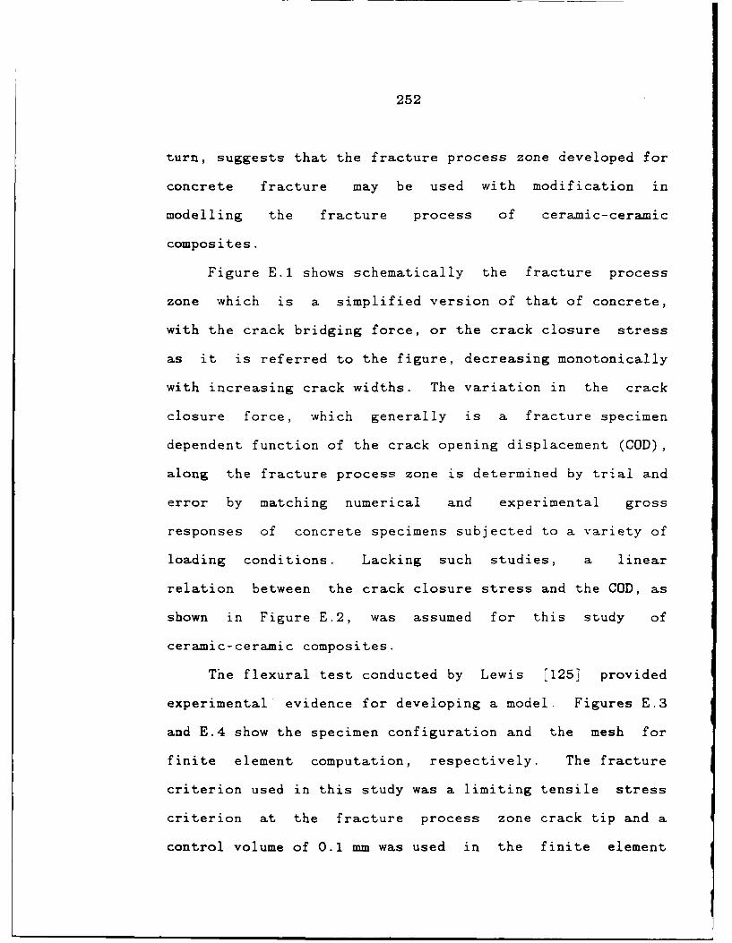
252
turn, suggests that the fracture process zone developed for
concrete fracture may be used with modification in
modelling the fracture process of ceramic-ceramic
composites.
Figure E.1 shows schematically the fracture process
zone which is a simplified version of that of concrete,
with the crack bridging force, or the crack closure stress
as it is referred to the figure, decreasing monotonically
with increasing crack widths. The variation in the crack
closure force, which generally is a fracture specimen
dependent function of the crack opening displacement (COD),
along the fracture process zone is determined by trial and
error by matching numerical and experimental gross
responses of concrete specimens subjected to a variety of
loading conditions. Lacking such studies, a linear
relation between the crack closure stress and the COD, as
shown in Figure E.2, was assumed for this study of
ceramic-ceramic composites.
The flexural test conducted by Lewis [125] provided
experimental evidence for developing a model. Figures E.3
and E.4 show the specimen configuration and the mesh for
finite element computation, respectively. The fracture
criterion used in this study was a limiting tensile stress
criterion at the fracture process zone crack tip and a
control volume of 0.1 mm was used in the finite element
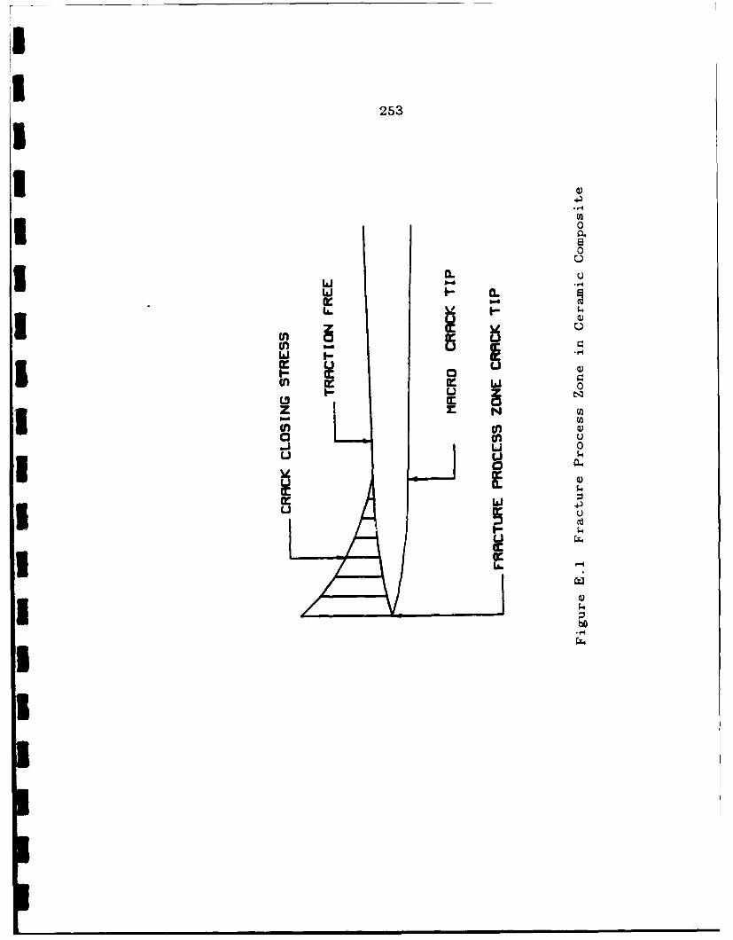
253
I0
0
IL-
w~ C L
0A 0
0 0)J LA
Is-I
CC
I bo
I-
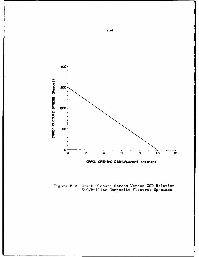
254
400-
I3 00-
10
0 2 4 6 8 10 1e
C OPENING DISPLIREMNT (Micron)
Figure E.2 Crack Closure Stress Versus COD RelationSiC/Mullite Composite Flexural Specimen
255
TENSILE STRENGTH 300 Pe
MODULUS OF ELASTICITY 400 Pe
POISSON'S RATIO ).35
gMm mM 5am
Figure E.3 SiC/Mullite Composite Flexural Specimen
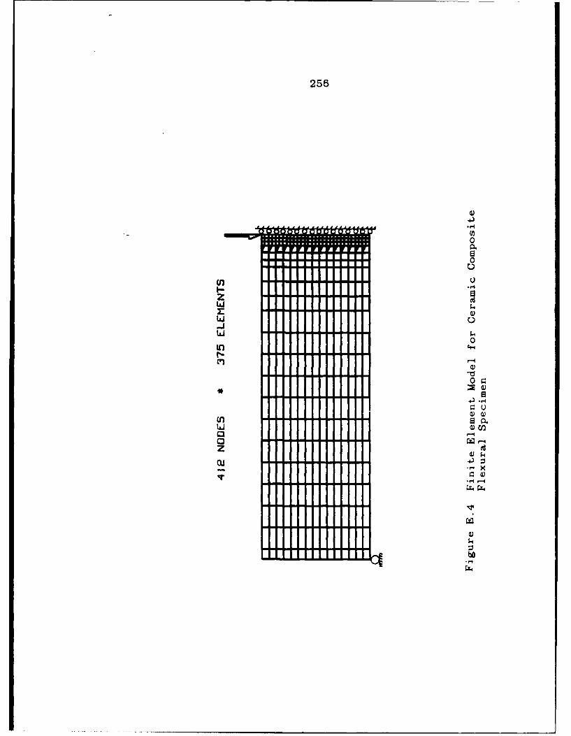
256
4)
0
ci,z
(4r 4)
a4 "
z ,4)
.r.
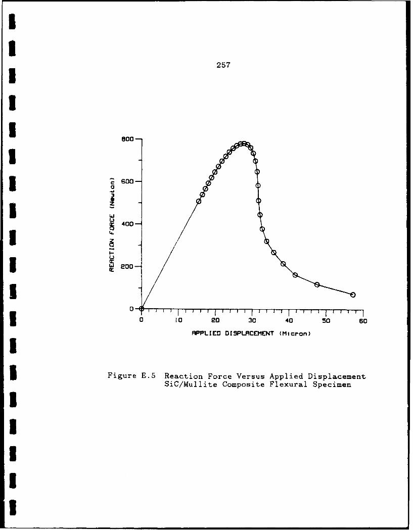
II
257II
I 800-
I
0600-
U400-3 eoo -
0 10 20 30 40 50 60
APPLIED DISPLACEMENT (Micron)I3Figure E.5 Reaction Force Versus Applied Displacement
SiC/Mullite Composite Flexural SpecimenII3II
258
computation. Shown in Figure E.5 is the load-displacement
curve for the flexural specimen under monotonic
displacement controlled loading. This curve, which is
commonly observed in concrete testing, exhibits a pre-peak
stiffness softening and a post-peak strength toughness.
The same specimen was tested under force controlled cyclic
loading to its maximum load-capacities. While the
monotonic loading response can be computed using finite
element methods incorporating a fracture process zone,
prediction of the unloading and reloading process requires
the development of a theoretical model additional to the
fracture process zone model discussed previously. The
assumptions used in developing such model were as follows:
1) In the unloading process, the material inside the
fracture process zone behaves linearly.
2) There is a stage in the middle of both unloading
and subsequent reloading phases at which the crack closure
stress in the fracture process zone vanishes and the
permanent deformation of the material in the fracture
process zone is evaluated at the corresponding load level.
3) The incremental extension of the macro-crack tip
after each loading cycle is determined by a crack opening
displacement criterion which, in this study, was assumed to
be 3 microns.
II
259
U Figure E.6 provides an explanation of the failure
process of ceramic composites under cyclic loading.
According to assumption 1), the unloading curve should be a
straight line as shown by AC in Figure E.6 (a). Due to the
existence of permanent deformation, the material in the
process zone undergoes tension and then compression.
Point B, in the figure, represents the neutral state which
3 is assumed in assumption 2. Figure E.6 (b) shows the pre-B
reloading curve which is the same as the unloading curve
*because crack extension during the previous cycle has no
effect on the compressive load capacity. Figure E.6 (c)
shows the incremental advance of the macro-crack tip in
3 accordance with the second assumption. The post-B
reloading curve which deviates from CA starting at B
3 following the second and third assumptions. The only
problem left is to find the position of B. As shown in
Figure E.6 (d), the curve OE is the load-deflection
1 ,relation for the case in which there is no crack closure
stress in the fracture pro ss zone. Obviously, the point
3 B should be on both curves OE and CA. Hence, point B is
the intersection of these two curves.
Figure E.7 shows how the cyclic load-deflection curves
3 were generated. The computation steps can be summarized as
the followings:
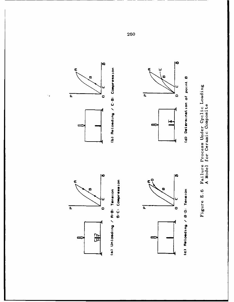
260
CL"CL C a.
A a1
cc 0
m o0
U - 4
C0 C
0
o a
u r ua, 9
.4(64
Q)
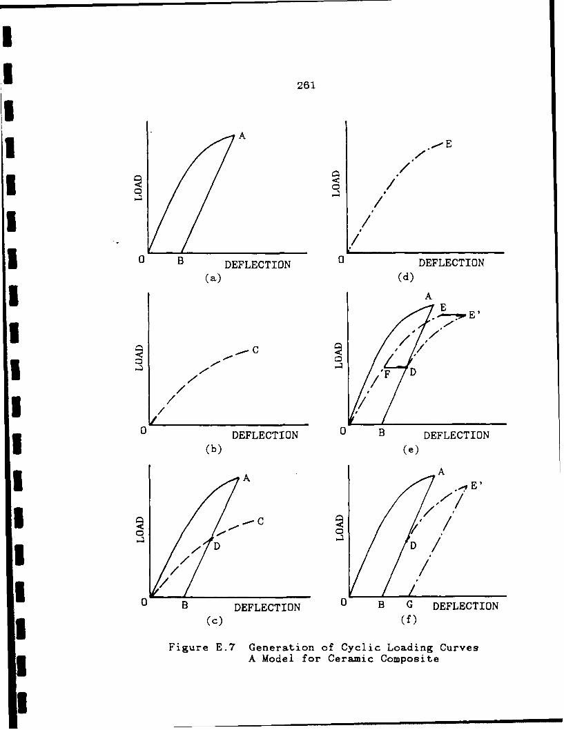
261
AI -AE
I /|//
1 0 B DEFLECTION 0 DEFLECTION
(a) (d)
A A
" E'
-C
co/
//
/
I / ,1
0 DEFLECTION 0 B DEFLECTION
A A
-C
0DEFLECTION 0 B G DEFLECTION3(c) (f)
Figure E.7 Generation of Cyclic Loading Curves3 A Model for Ceramic Composite

262
(a) The first cycle of load versus deflection curve
was computed using the fracture process zone model for
loading process and assumption 1) for unloading process.
The result is shown in Figure E.7 (a) as QAB.
(b) Without prescribing any crack closure stress on
the microcrack surfaces load versus deflection curve was
re-computed and shown in Figure E.7 (b) as OC.
(c) The "neutral point", thus, was determined as to
be the intersection of AB and 0C shown in Figure E.7 (c) as
D.
(d) The second cycle of load versus deflection curve
was then computed with an advancement of traction free
crack according to assumption 3). The result is shown in
Figure E.7 (d).
(e) Cu_'ve EF was translated Horizontally to E'D as
shown in Figure E.7 (e). The length of EE' is the same as
that of FD.
(f) The second cycle of load versus deflection curve
was completed by drawing a straight line E'G whose slope is
the same as that of curve OF at point 0 as shown in
Figure E.7 (f).
Figure E.8 presents the final result which is in good
agreement with the test result [125]. Since the actual
test result was reproduced by numerical computation based
on a postulated model, the model was verified.
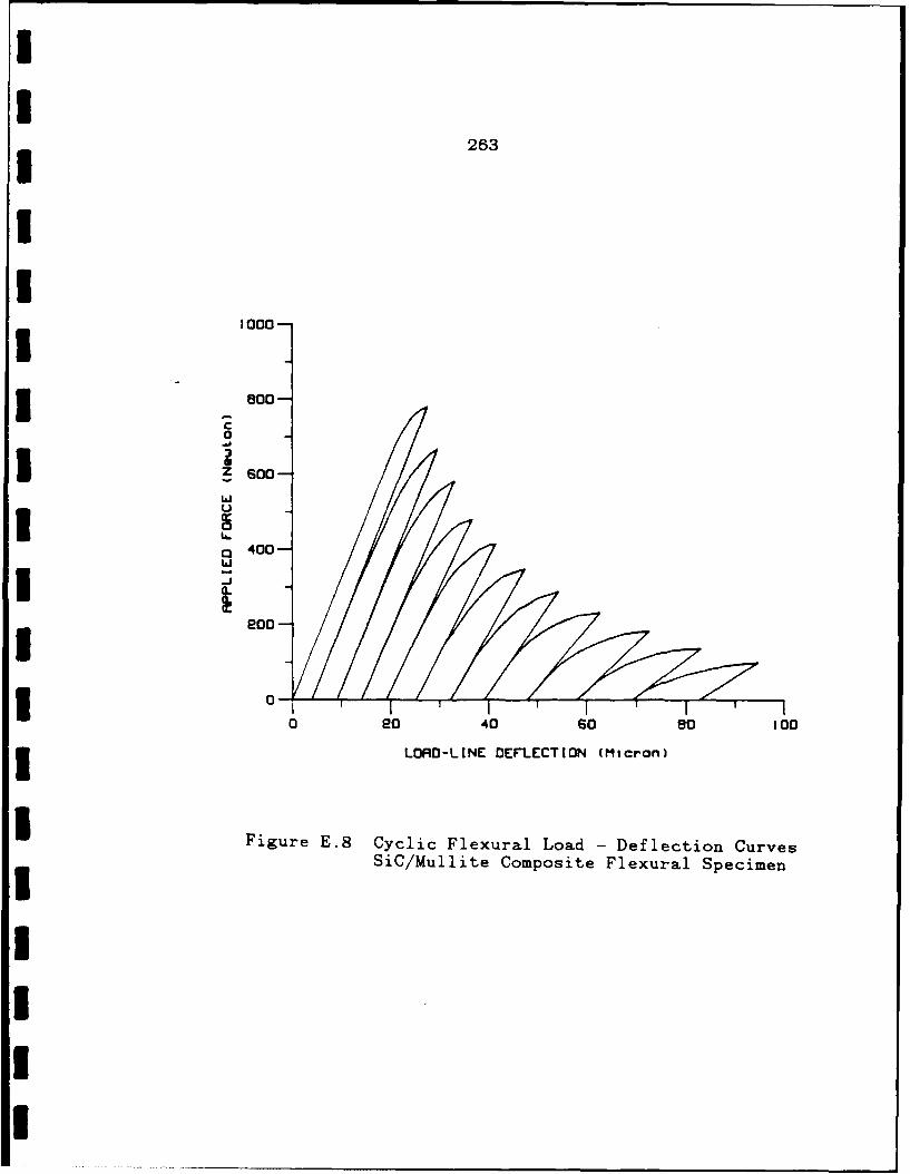
1 263
1000-
1 800-
I1 3600-
I U
S400-
I -
10-0 20 40 s0 80 1003 LORD-LINE DEFLECTION (Micron)
I Figure E.8 Cyclic Flexural Load - Deflection CurvesSiC/Mullite Composite Flexural Specimen
264
Shown in Figure E.9 are computed load versus
deflection relationship for specimens with differing
prenotched lengths and in Figure E.lO are computed crack
profiles for a propagating crack in a specimen without a
prenotch. These theoretical predictions can be used later
-to verify this model whenever test results become available
for such comparisons.
Obviously, similar modeling analysis can be carried
out for concrete and a more detailed treatment developed
for studying the failure mechanism of a material during the
unloading and reloading phases of low cycle fatigue
testing.
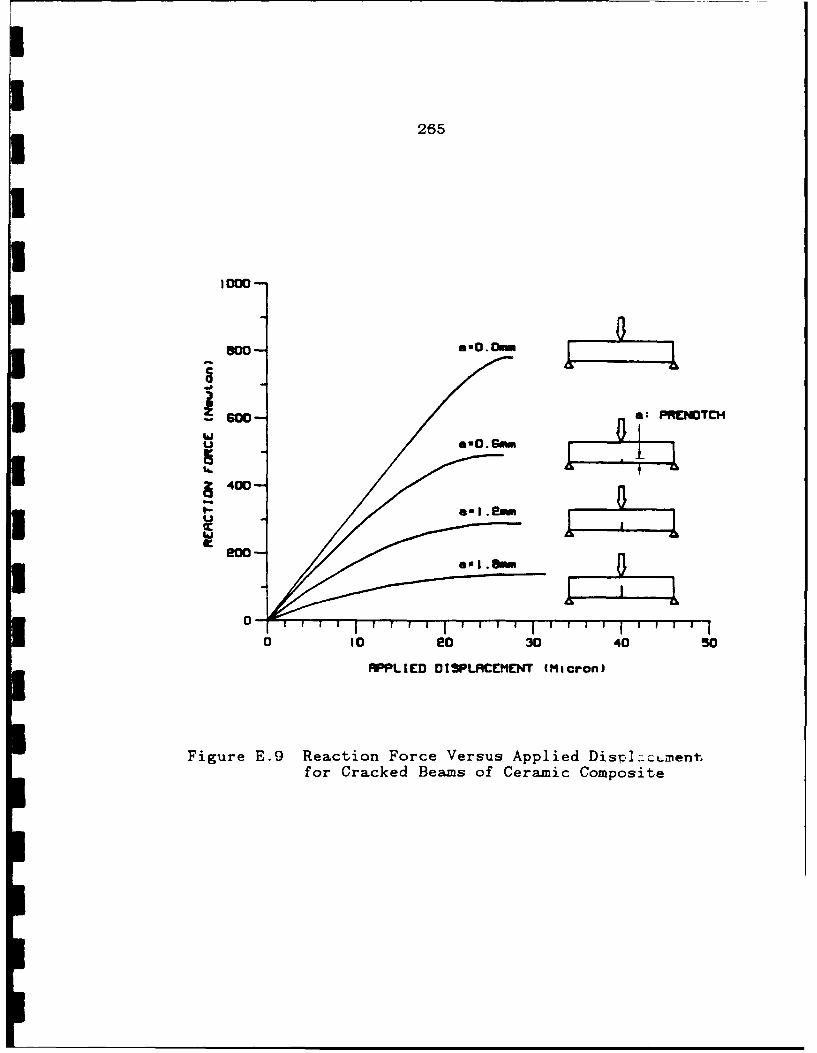
265
1000-
80- S'° 0 ____
0
~60O *:PRENOTCH
~400-
0-
0 1O 20 30 40 50
APPLIED O1SPLRCEMENT (Micron)
Figure E.9 Reaction Force Versus Applied Displazt-nmentfor Cracked Beams of Ceramic Composite
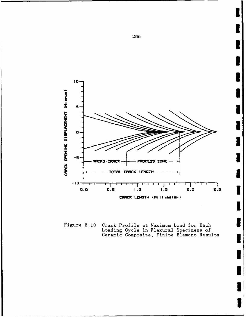
266
0I
-103
0.0 0.I. . ~ .
CRAC LENTH (illieterFgur -0 CakPrfl tMxmu0odfrEc
Lodn CylInFeualSeieso
CermicComosteFinte leentReslt
III3 APPENDIX F
KR CURVE RE-EVALUATION BASED ON TEST RESULTS
IThe method of evaluation of KR values for Crack-Line
I Wedge-Loaded Double-Cantilever Beam (CLWL-DCB) specimens of
metals is given in ASTM Standard 561-81 [115]. This method
was applied to the CLWL-DCB concrete specimens by Jeang [9]
3 in 1985 at the University of Washington. Recently, Jeang's
results have been re-evaluated, and based on the fracture
I process zone model reported here, new values for K were
derived.
In ASTM Standard 561-81, crack opening displacememts
3 at 2 specific locations on the crack line, termed 2V 1 and
2V2 , are to be measured. rlhen, the ratio of 2V I to 2V2 is
3 used to obtain the effective crack length by consulting a
table in the Standard. Finally, the KR value, is computed
using a formula of LEFM, for which the measured wedge load
3 value and the effective crack length value are input data.
Jeang conducted 5 groups of concrete CLWL-DCB tests with
3 different concrete compressive strengths, aggregate sizes
and specimen sizes, He substituted his measured 2VI /2V2
and wedge load values into the table and the formula in the
3 Standard and obtained values for KR' Data points on a KR
versus effective crack length diagram showed con. Through
3 regression processing, the curves which were appropriate
268
second degree polynominals of best fit to the data points
were obtained. These results were presented in Jeang's [9]
dissertation as Figure 4.20. Since KR values were not
measured, Jeang's results are only partial-test results.
Standard 561-81 is intended for metals only, not
.-concrete. In order to determine if the ASTM Standard
applies to concrete and can be used to obtain KR values for
CLWL-DCB specimens of concrete, a finite element analysis
was conducted on the computer. The fracture process zone
model was incorporated into that finite element program and
along with the experimental data reported in Jeang's
dissertation. Analyses were carried out in two ways.
First, Jeang's procedure was followed except that computed
2V1' 2V 2 and wedge load values were used for input rather
than the measured data. The computation results are shown
in Figures F.1 through F.5 by the dashed lines. Second, an
energy analysis was performed by evaluating the fracture
energy (work of fracture) dissipation rate within the
fracture process zone as the microcrack tip advanced.
Then, the fracture energy rate was converted to KR through
the following relationship:
KR = (E*G/(1-v)) (for plane strain)
in which E, V, and G are Young's modulus, Poisson's Ratio
and fracture energy rate, respectively. The results
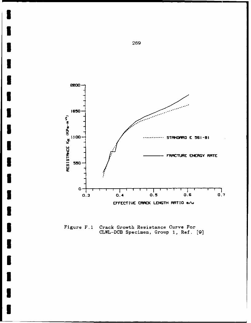
II
269
N
I1650-
I "S.
1100 ------------ STRF'N ARD E 561-81
U
E FRRCTLJRE ENERGY RATEI in
0 - I
0.3 0.4 0.5 0.6 0.7
EFFECTIVE CRIC LENGTH RATIO e/wI* Figure F.1 Crack Growth Resistance Curve For
CLWL-DCB Specimen, Group 1, Ref. [9]
IIIII
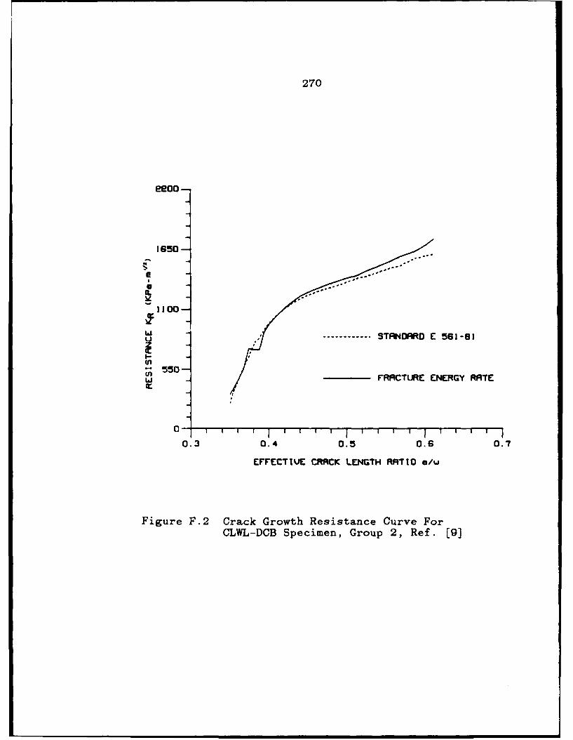
270
eeoo
1650"
1100
........ STANDARD E 561-81
i 56 B
550 --FRACTURE ENERGY RATE
0-
0.3 0.4 0.5 0.6 0.7
EFFECTIVE CRACK LENGTH RATIO e/w
Figure F.2 Crack Growth Resistance Curve ForCLWL-DCB Specimen, Group 2, Ref. [9]
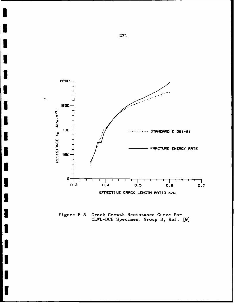
271
eeoo-
3 1650-I 0.
I100 " STANDD E 561-81
U
FRACTURE ENERGY RATE
U550
II0.3 0.4 0.5 0.6 0.7
EFFECTIVE CRACK LENGTH RATIO e/w
I
I Figure F.3 Crack Growth Resistance Curve ForCLWL-DCB Specimen, Group 3, Ref. [9]I
IIII
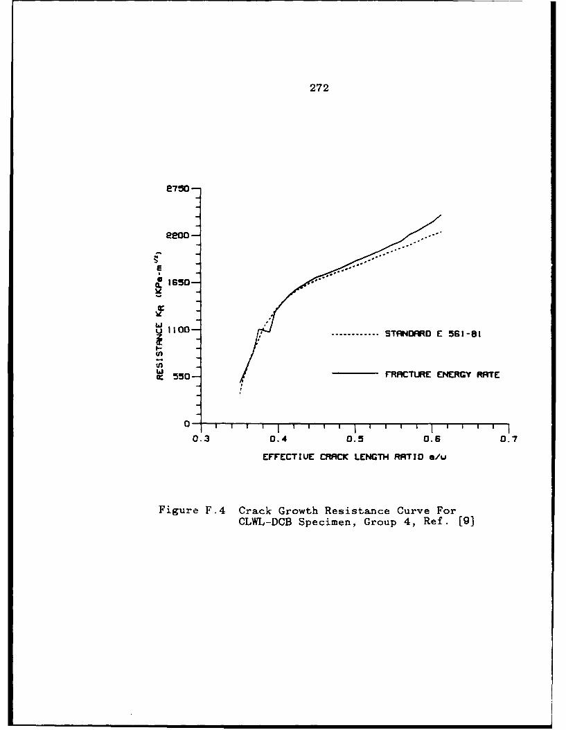
272
2750-
eeoo -
L 1650-
U 1100-- ............ STRNOARO E 561-81
W FRACTURE ENERGY RATES550-
0 - ' ' I j I I I I j I
0.3 0.4 0.5 0.6 0.7
EFFECTIVE CRACK LENGTH RATIO G/u
Figure F.4 Crack Growth Resistance Curve ForCLWL-DCB Specimen, Group 4, Ref. [9]
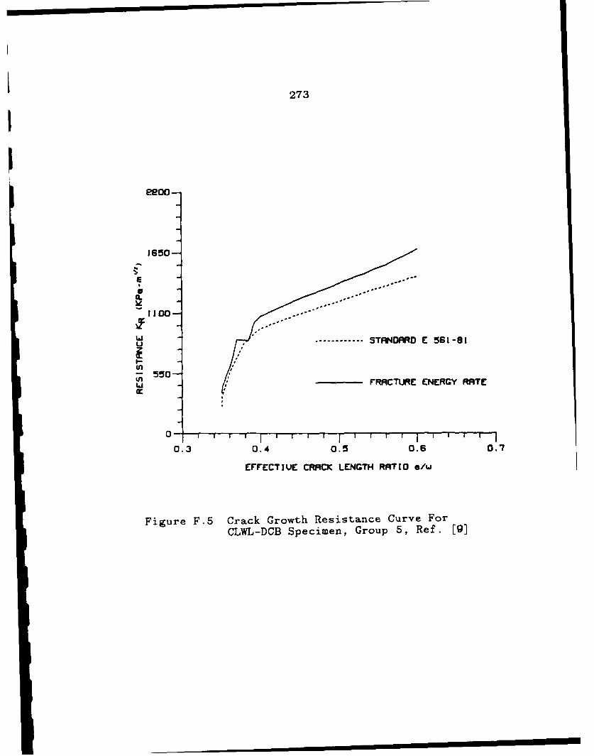
273
eeoo-
1650
E
0.
1100
....... STANODR0 E 561 -81
(n550- RACTURE ENER~GY RATE
0.3 0.4 0.5 0.6 0.7
EFFECTIVE CRROC LENGTH RRIIO G/u
Figure F.5 Crack Growth Resistance Curve ForCLWL-DCB Specimen, Group 5, Ref. [9]
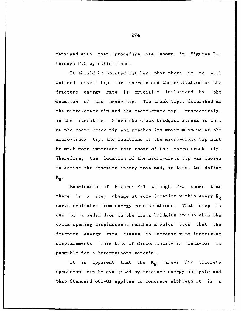
274
obtained with that procedure are shown in Figures F-1
through F.5 by solid lines.
It should be pointed out here that there is no well
defined crack tip for concrete and the evaluation of the
fracture energy rate is crucially influenced by the
-location of the crack tip. Two crack tips, described as
the micro-crack tip and the macro-crack tip, respectively,
in the literature. Since the crack bridging stress is zero
at the macro-crack tip and reaches its maximum value at the
micro-crack tip, the locations of the micro-crack tip must
be much more important than those of the macro-crack tip.
T1herefore, the location of the micro-crack tip was chosen
to define the fracture energy rate and, in turn, to define
KR.
Examination of Figures F-i through F-5 shows that
there is a step change at some location within every KR
curve evaluated from energy considerations. That step is
due to a suden drop in the crack bridging stress when the
crack opening displacement reaches a value such that the
fracture energy rate ceases to increase with increasing
displacements. This kind of discontinuity in behavior is
possible for a heterogenous material.
It is apparent that the KR values for concrete
specimens can be evaluated by fracture energy analysis and
that Standard 561-81 applies to concrete although it is a

II
275
IU little conservative.
IIIIIIIIIIIIIII