Ocean Sci., 14, 1603–1618, 2018https://doi.org/10.5194/os-14-1603-2018© Author(s) 2018. This work is distributed underthe Creative Commons Attribution 4.0 License.

Hydrography, transport and mixing of the West SpitsbergenCurrent: the Svalbard Branch in summer 2015Eivind Kolås and Ilker FerGeophysical Institute, University of Bergen, Bergen, Norway

Correspondence: Ilker Fer (ilker.fer@uib.no)

Received: 17 July 2018 – Discussion started: 17 August 2018Revised: 19 November 2018 – Accepted: 7 December 2018 – Published: 21 December 2018

Abstract. Measurements of ocean currents, stratification andmicrostructure were made in August 2015, northwest ofSvalbard, downstream of the Atlantic inflow in Fram Straitin the Arctic Ocean. Observations in three sections are usedto characterize the evolution of the West Spitsbergen Cur-rent (WSC) along a 170 km downstream distance. Two al-ternative calculations imply 1.5 to 2 Sv (1 Sv = 106 m3 s−1)is routed to recirculation and Yermak branch in Fram Strait,whereas 0.6 to 1.3 Sv is carried by the Svalbard branch. TheWSC cools at a rate of 0.20 ◦C per 100 km, with associ-ated bulk heat loss per along-path meter of (1.1− 1.4)×107 W m−1, corresponding to a surface heat loss of 380–550 W m−2. The measured turbulent heat flux is too smallto account for this cooling rate. Estimates using a plausiblerange of parameters suggest that the contribution of diffusionby eddies could be limited to one half of the observed heatloss. In addition to shear-driven mixing beneath the WSCcore, we observe energetic convective mixing of an unsta-ble bottom boundary layer on the slope, driven by Ekmanadvection of buoyant water across the slope. The estimatedlateral buoyancy flux isO(10−8)W kg−1, sufficient to main-tain a large fraction of the observed dissipation rates, andcorresponds to a heat flux of approximately 40 W m−2. Weconclude that – at least in summer – convectively driven bot-tom mixing followed by the detachment of the mixed fluidand its transfer into the ocean interior can lead to substantialcooling and freshening of the WSC.

1 Introduction

The Arctic Ocean contributes to the global ocean thermoha-line circulation through exchanges in Fram Strait, which is

the main connection to the Atlantic Ocean (Aagaard et al.,1985). The total volume transport through Fram Strait is9±2 Sv (1 Sv= 106 m3 s−1) northward and 12±1 Sv south-ward (Fahrbach et al., 2001; Schauer et al., 2004). A largefraction of the northward flow is the West Spitsbergen Cur-rent (WSC), located on the eastern side of Fram Strait, whichis a northward-flowing extension of the Norwegian AtlanticCurrent. The mean net volume transport in the WSC, mea-sured along an array at 78◦50′ N in the period between 1997and 2010, is 6.6± 0.4 Sv (Beszczynska-Möller et al., 2012),of which 3.0± 0.2 Sv is Atlantic Water (AW) with a tem-perature above 2 ◦C. The WSC continues as a topographi-cally guided boundary current, contributing to the circum-polar boundary current downstream. Between Fram Straitand the Lomonosov Ridge, the boundary current slows downfrom about 0.25 to 0.06 m s−1 and changes structure froma mainly barotropic flow to a baroclinic flow (Pnyushkovet al., 2015). AW transported by the WSC is the major heatand salinity source for the Arctic Ocean (Boyd and D’Asaro,1994; Aagaard et al., 1985; Rudels et al., 2015), and Arcticconditions are highly influenced by changes in the AW inflowproperties (Polyakov et al., 2017).

The circulation of AW in Fram Strait has multiplebranches (Fig. 1a). The WSC flows at a steady pace ofapproximately 0.25 m s−1, along the 1000 m isobath, fromBear Island at 74◦30′ N to the southern flanks of the YermakPlateau (YP) at 79◦30′ N (Boyd and D’Asaro, 1994). Obser-vations show that the WSC splits into two branches where theisobaths diverge near the YP, an outer branch following the1000 m isobath, and an inner branch (the Svalbard branch)following the 400 m isobath (Aagaard et al., 1987; Farrellyet al., 1985; Cokelet et al., 2008). The Svalbard branch hasa 40 km wide core with a strong barotropic component and

Published by Copernicus Publications on behalf of the European Geosciences Union.

1604 E. Kolås and I. Fer: Mixing of the West Spitsbergen Current

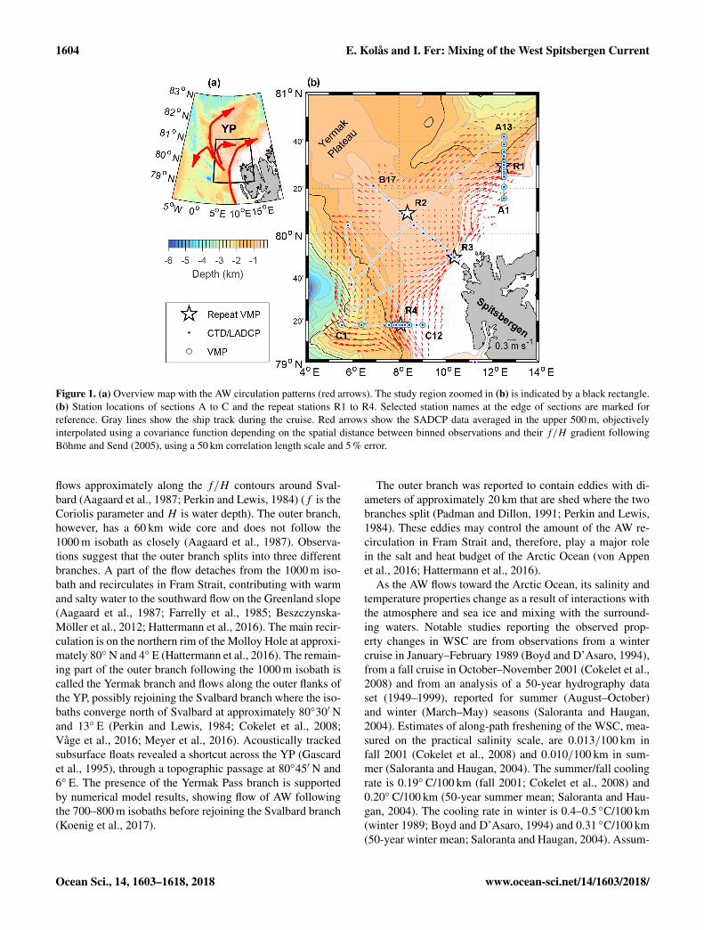
Figure 1. (a) Overview map with the AW circulation patterns (red arrows). The study region zoomed in (b) is indicated by a black rectangle.(b) Station locations of sections A to C and the repeat stations R1 to R4. Selected station names at the edge of sections are marked forreference. Gray lines show the ship track during the cruise. Red arrows show the SADCP data averaged in the upper 500 m, objectivelyinterpolated using a covariance function depending on the spatial distance between binned observations and their f/H gradient followingBöhme and Send (2005), using a 50 km correlation length scale and 5 % error.

flows approximately along the f/H contours around Sval-bard (Aagaard et al., 1987; Perkin and Lewis, 1984) (f is theCoriolis parameter and H is water depth). The outer branch,however, has a 60 km wide core and does not follow the1000 m isobath as closely (Aagaard et al., 1987). Observa-tions suggest that the outer branch splits into three differentbranches. A part of the flow detaches from the 1000 m iso-bath and recirculates in Fram Strait, contributing with warmand salty water to the southward flow on the Greenland slope(Aagaard et al., 1987; Farrelly et al., 1985; Beszczynska-Möller et al., 2012; Hattermann et al., 2016). The main recir-culation is on the northern rim of the Molloy Hole at approxi-mately 80◦ N and 4◦ E (Hattermann et al., 2016). The remain-ing part of the outer branch following the 1000 m isobath iscalled the Yermak branch and flows along the outer flanks ofthe YP, possibly rejoining the Svalbard branch where the iso-baths converge north of Svalbard at approximately 80◦30′ Nand 13◦ E (Perkin and Lewis, 1984; Cokelet et al., 2008;Våge et al., 2016; Meyer et al., 2016). Acoustically trackedsubsurface floats revealed a shortcut across the YP (Gascardet al., 1995), through a topographic passage at 80◦45′ N and6◦ E. The presence of the Yermak Pass branch is supportedby numerical model results, showing flow of AW followingthe 700–800 m isobaths before rejoining the Svalbard branch(Koenig et al., 2017).

The outer branch was reported to contain eddies with di-ameters of approximately 20 km that are shed where the twobranches split (Padman and Dillon, 1991; Perkin and Lewis,1984). These eddies may control the amount of the AW re-circulation in Fram Strait and, therefore, play a major rolein the salt and heat budget of the Arctic Ocean (von Appenet al., 2016; Hattermann et al., 2016).

As the AW flows toward the Arctic Ocean, its salinity andtemperature properties change as a result of interactions withthe atmosphere and sea ice and mixing with the surround-ing waters. Notable studies reporting the observed prop-erty changes in WSC are from observations from a wintercruise in January–February 1989 (Boyd and D’Asaro, 1994),from a fall cruise in October–November 2001 (Cokelet et al.,2008) and from an analysis of a 50-year hydrography dataset (1949–1999), reported for summer (August–October)and winter (March–May) seasons (Saloranta and Haugan,2004). Estimates of along-path freshening of the WSC, mea-sured on the practical salinity scale, are 0.013/100 km infall 2001 (Cokelet et al., 2008) and 0.010/100 km in sum-mer (Saloranta and Haugan, 2004). The summer/fall coolingrate is 0.19◦ C/100 km (fall 2001; Cokelet et al., 2008) and0.20◦ C/100 km (50-year summer mean; Saloranta and Hau-gan, 2004). The cooling rate in winter is 0.4–0.5 ◦C/100 km(winter 1989; Boyd and D’Asaro, 1994) and 0.31 ◦C/100 km(50-year winter mean; Saloranta and Haugan, 2004). Assum-

Ocean Sci., 14, 1603–1618, 2018 www.ocean-sci.net/14/1603/2018/

E. Kolås and I. Fer: Mixing of the West Spitsbergen Current 1605

ing an AW layer between 100 and 500 m depth, the coolingrate is equivalent to a heat loss of 310–330 W m−2 in summer(Aagaard et al., 1987; Saloranta and Haugan, 2004; Cokeletet al., 2008) and 1050 W m−2 in winter (Saloranta and Hau-gan, 2004). The cooling of the WSC stream tube observed inwinter 1989 implies approximately 900 W m−2, limited to a22 km wide core (Boyd and D’Asaro, 1994). Note that theseheat losses are dependent on the mean advective speed, thatis the residence time of the water in the area of cooling.

Boyd and D’Asaro (1994) describe the cooling of theWSC in winter as a three-stage process: cooling by the at-mosphere, cooling by sea ice and cooling by eddy-drivenmixing along isopycnals. The relative role of the differentcooling processes is not clear. Numerical linear stability anal-yses using idealized current profile and topography suggestthat heat loss contribution from isopycnal diffusion as a re-sult of barotropic instability corresponds to an along-shelfcooling rate of 0.08 ◦C/100 km (Teigen et al., 2010). The ex-tension of the analysis to a two-layer model shows that thebaroclinic instability occurs, most pronounced during win-ter/spring, leading to a heat loss reaching 240 W m−2, fromthe core of the WSC to the atmosphere (Teigen et al., 2011).

All these studies agree that vertical mixing alone cannotaccount for the observed cooling rates. Fer et al. (2010) con-clude that internal-wave activity and mixing show variabilityrelated to topography and hydrography; thus, the path of theWSC will affect the cooling and freshening rates the AW ex-periences. Over the steep slopes and prominent topographyof the YP, and over the core of the AW branches, verticalmixing can play an important role in modifying the AW prop-erties (Padman and Dillon, 1991; Meyer et al., 2016; Sire-vaag and Fer, 2009). In the surface mixed layer in proxim-ity to the WSC, turbulent heat fluxes of O(100) W m−2 weremeasured (Sirevaag and Fer, 2009). Once the AW subducts,the vertical mixing is suppressed by the overlaying strongstratification, reducing the heat loss to the atmosphere or seaice. Padman and Dillon (1991) observed a time-averaged up-ward heat flux in the pycnocline above the Atlantic layer of25 W m−2 over the YP slope, of which only about 6 W m−2

actually entered the mixed layer. At the core of the Svalbardbranch, Fer et al. (2010) observed that near-bottom mixingremoved 15 W m−2 from the AW layer to cold waters be-low. Outside the WSC, near the northeastern flank of the YP,Sirevaag and Fer (2009) found an average vertical heat fluxof 2 W m−2, comparable to the annual oceanic heat flux of3–4 W m−2 to the Arctic pack ice (Krishfield and Perovich,2005).

Here we report summer observations of ocean stratifica-tion, currents and microstructure from north of Svalbard nearthe YP, collected during a cruise in August 2015. Using threesections across the WSC, we present the background cur-rents, volume and heat transport and their evolution along thepath of WSC. Vertical mixing and heat loss from the WSCare quantified. The goal of this study is to improve the gen-eral understanding of processes modifying the Atlantic Wa-

ter inflow into the Arctic Ocean and to describe the impor-tance of vertical mixing versus horizontal processes duringsummer. We propose that convective mixing in the bottomboundary layer and the subsequent lateral export of mixedwater can make a substantial contribution to the cooling rateof the WSC.

2 Data

The data set analyzed in this study was collected from theresearch vessel (R/V) Håkon Mosby between 12 and 21 Au-gust 2015. The ship track and the locations of the differentstations are shown in Fig. 1b. Data were collected mainlyalong three sections, referred to as sections A–C, using theconductivity–temperature–depth (CTD) and lowered acous-tic Doppler current profiler (LADCP) system, the verticalmicrostructure profiler (VMP) and the shipboard acousticDoppler current profiler (SADCP). The sampling durationof sections A–C was approximately 20, 11 and 20 h, respec-tively. It took 5 days from the sampling started on section Ato the end of C. Our results discussed in Sect. 4 assume thatthe conditions of the inner branch of the WSC do not changesignificantly during these 5 days, thus giving a synoptic view.In total, 46 CTD/LADCP and 85 VMP profiles are analyzed.

2.1 Temperature and salinity measurements

The CTD profiles were acquired using a Sea-Bird Scientific,SBE 911plus system. A 200 kHz Benthos altimeter allowedprofiles to within 10 m of the seabed. The CTD system wasalso equipped with a WET Labs C-Star transmissometer.Accuracy of the pressure, temperature and salinity sensorsare ±0.5 dbar, ±2× 10−3 ◦C and ±3× 10−3, respectively.The CTD data are processed using the SBE software fol-lowing the recommended procedures. Conservative temper-ature, 2, and absolute salinity, SA, are calculated using thethermodynamic equation of seawater (IOC et al., 2010), andthe Gibbs SeaWater (GSW) Oceanographic Toolbox (Mc-Dougall and Barker, 2011).

2.2 Current measurements

Horizontal current profile measurements were made usingthe LADCP and SADCP systems. All current measurementsare corrected for the magnetic declination. Two 300 kHzTeledyne RD Instruments Workhorse LADCPs were in-stalled on the CTD rosette collecting 1 s profiles in master–slave mode to ensure synchronization. The sampling verticalbin size was set to 8 m for each acoustic Doppler current pro-filer (ADCP). The LADCP data are processed as 8 m verti-cal averages using both ADCPs and both up- and downcasts,and using the Lamont-Doherty Earth Observatory (LDEO)Software version IX.12, which is an implementation of thevelocity inversion method described in Visbeck (2002). Pro-files are obtained using the constraints from velocities from

www.ocean-sci.net/14/1603/2018/ Ocean Sci., 14, 1603–1618, 2018

1606 E. Kolås and I. Fer: Mixing of the West Spitsbergen Current

ship navigation, bottom tracking and SADCP, with a result-ing horizontal velocity error of less than 3 cm s−1 (Thurnherr,2010).

SADCP on R/V Håkon Mosby was a 75 kHz Teledyne RDInstruments Ocean Surveyor. It collected velocity profilescontinuously in the broadband mode. Final profiles, 5 mintime-averaged, are obtained using the University of Hawaiisoftware (Firing et al., 1995). Typical final processed hori-zontal velocity uncertainty is 2–3 cm s−1.

2.3 Microstructure measurements

Ocean microstructure measurements were made using a2000 m rated VMP manufactured by Rockland Scientific,Canada (RSI). The VMP is a loosely tethered profiler witha nominal sink velocity of 0.6 m s−1. The profiler wasequipped with pumped SBE-CT sensors, a pressure sensor,microstructure velocity shear probes, one high-resolutiontemperature sensor, one high-resolution micro-conductivitysensor and three accelerometers.

The processing of the microstructure data is based onthe routines provided by RSI (ODAS v4.01) (Douglas andLueck, 2015). Assuming isotropic turbulence, the dissipationrate of turbulent kinetic energy (TKE) per unit mass can beexpressed as

ε =152ν

(∂u

∂z

)2

, (1)

where ν is the kinematic viscosity, overbar denotes averag-ing in time and the ∂u/∂z is the small-scale shear of one hor-izontal velocity component u. Using a constant fall rate ofthe instrument and invoking the frozen turbulence hypothe-sis over an analysis time of several seconds, the term with theoverbar represents the shear variance from order 1 m verticalscale to order 1 cm scales where dissipation occurs. Dissipa-tion rates are calculated from the shear variance obtained byintegrating the shear wave number spectra, using 1 s Fouriertransform length length and half-overlapping 4 s segments,following the corrections and methods described in theRSI Technical Notes (https://rocklandscientific.com/support/knowledge-base/technical-notes/, last access: 2 July 2018).Resulting values are quality-screened by inspecting the in-strument accelerometer records and individual spectra fromthe two shear probes. Estimates from both probes are aver-aged when they agree to within a factor of 10. Otherwise, thelower dissipation value is accepted because larger values canbe caused by spikes induced, e.g., by impact with plankton.

3 Methods

3.1 Water masses

We use the classical categorization of water masses in the re-gion, as first defined by Swift and Aagaard (1981) and later

modified by Aagaard et al. (1985), listed in Table 1. Note,however, that changes in the properties and distribution ofthe intermediate and deep waters in Fram Strait were ob-served, and discussed in Langehaug and Falck (2012). Theabsolute salinity, SA, in Table 1 is calculated from the prac-tical salinity values at 80◦ N and 10◦ E and rounded to thenearest hundredth.

3.2 Tidal currents and geostrophic currents

The barotropic tidal current components in the LADCP andSADCP profiles are removed using the 5 km horizontal reso-lution Arctic Ocean Tidal Inverse Model, AOTIM-5 (Padmanand Erofeeva, 2004). The tidal transport at specified latitudeand longitude coordinates is predicted for the mid-time of thecurrent profiles, and the barotropic tidal current is obtainedby dividing by the water depth at that specific location. Atthe CTD/LADCP stations (Fig. 1), where station depth is ac-curately measured, the measured station depth is used. Thewater depth elsewhere (for SADCP) is obtained from the In-ternational Bathymetric Chart of the Arctic Ocean (IBCAO)database (Jakobsson et al., 2012).

Hydrography and current profiles collected along the threesections are gridded to 2 m vertical and 1 km horizontal dis-tance, using linear interpolation. After uniformly griddingthe data, a moving average smoothing is performed usinga 10 km× 10 m (horizontal× vertical) window. While thesmoothing removes the short timescale and length scale vari-ability, it does not necessarily remove all ageostrophic vari-ability.

Dynamic height anomaly and the geostrophic currents arecalculated relative to a reference pressure of 100 dbar fromthe gridded and smoothed SA and 2 fields. The referencepressure is chosen so that it is away from frictional bound-ary layers where ageostrophic currents can be substantial.The absolute geostrophic velocity is then obtained by addingthe across-section component of the observed currents at thereference level. The observed currents used are the de-tidedLADCP profiles, identically gridded and smoothed as the hy-drographic fields for consistency.

3.3 Stream tubes

The stream tube of WSC is defined using the absolutegeostrophic velocities in the AW layer. The vertical extent ofthe tube is defined by the AW layer (or seabed). The horizon-tal center of the stream tube on a section is defined as the lo-cation of the maximum layer-integrated velocity (i.e., trans-port density, m2 s−1) and assigned x = 0 km (see Figs. 5and 6). The lateral extent of the stream tube is defined intwo alternative ways.

In the first alternative (stream tube 1), the horizontalbounds are identified on either side of the core, as the locationwhere the transport density first drops below a backgroundthreshold (solid enclosed curves in Figs. 2–4). The thresh-

Ocean Sci., 14, 1603–1618, 2018 www.ocean-sci.net/14/1603/2018/

E. Kolås and I. Fer: Mixing of the West Spitsbergen Current 1607

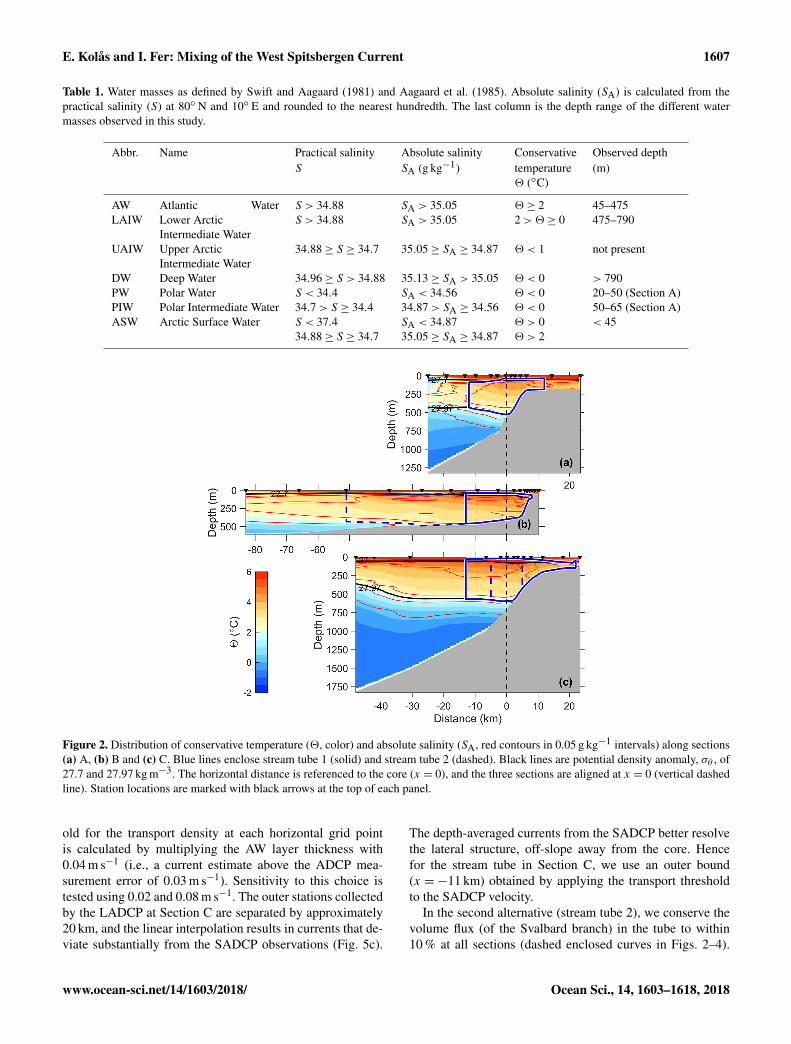
Table 1. Water masses as defined by Swift and Aagaard (1981) and Aagaard et al. (1985). Absolute salinity (SA) is calculated from thepractical salinity (S) at 80◦ N and 10◦ E and rounded to the nearest hundredth. The last column is the depth range of the different watermasses observed in this study.

Abbr. Name Practical salinity Absolute salinity Conservative Observed depthS SA (g kg−1) temperature (m)

2 (◦C)

AW Atlantic Water S > 34.88 SA > 35.05 2≥ 2 45–475LAIW Lower Arctic S > 34.88 SA > 35.05 2>2≥ 0 475–790

Intermediate WaterUAIW Upper Arctic 34.88≥ S ≥ 34.7 35.05≥ SA ≥ 34.87 2< 1 not present

Intermediate WaterDW Deep Water 34.96≥ S > 34.88 35.13≥ SA > 35.05 2< 0 > 790PW Polar Water S < 34.4 SA < 34.56 2< 0 20–50 (Section A)PIW Polar Intermediate Water 34.7> S ≥ 34.4 34.87> SA ≥ 34.56 2< 0 50–65 (Section A)ASW Arctic Surface Water S < 37.4 SA < 34.87 2> 0 < 45

34.88≥ S ≥ 34.7 35.05≥ SA ≥ 34.87 2> 2

Figure 2. Distribution of conservative temperature (2, color) and absolute salinity (SA, red contours in 0.05 g kg−1 intervals) along sections(a) A, (b) B and (c) C. Blue lines enclose stream tube 1 (solid) and stream tube 2 (dashed). Black lines are potential density anomaly, σθ , of27.7 and 27.97 kg m−3. The horizontal distance is referenced to the core (x = 0), and the three sections are aligned at x = 0 (vertical dashedline). Station locations are marked with black arrows at the top of each panel.

old for the transport density at each horizontal grid pointis calculated by multiplying the AW layer thickness with0.04 m s−1 (i.e., a current estimate above the ADCP mea-surement error of 0.03 m s−1). Sensitivity to this choice istested using 0.02 and 0.08 m s−1. The outer stations collectedby the LADCP at Section C are separated by approximately20 km, and the linear interpolation results in currents that de-viate substantially from the SADCP observations (Fig. 5c).

The depth-averaged currents from the SADCP better resolvethe lateral structure, off-slope away from the core. Hencefor the stream tube in Section C, we use an outer bound(x =−11 km) obtained by applying the transport thresholdto the SADCP velocity.

In the second alternative (stream tube 2), we conserve thevolume flux (of the Svalbard branch) in the tube to within10 % at all sections (dashed enclosed curves in Figs. 2–4).

www.ocean-sci.net/14/1603/2018/ Ocean Sci., 14, 1603–1618, 2018

1608 E. Kolås and I. Fer: Mixing of the West Spitsbergen Current

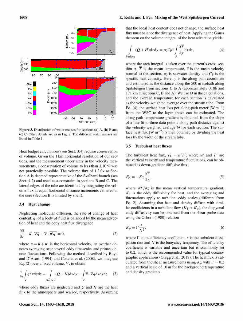
Figure 3. Distribution of water masses for sections (a) A, (b) B and(c) C. Other details are as in Fig. 2. The different water masses arelisted in Table 1.

Heat budget calculations (see Sect. 3.4) require conservationof volume. Given the 1 km horizontal resolution of our sec-tions, and the measurement uncertainty in the velocity mea-surements, a conservation of volume to less than ±10 % wasnot practically possible. The volume flux of 1.3 Sv at Sec-tion A is deemed representative of the Svalbard branch (seeSect. 4.2) and used as a constraint in sections B and C. Thelateral edges of the tube are identified by integrating the vol-ume flux at equal horizontal distance increments centered atthe core (Section B is limited by shelf).

3.4 Heat change

Neglecting molecular diffusion, the rate of change of heatcontent, q, of a body of fluid is balanced by the mean advec-tion of heat and the eddy heat flux divergence

∂q

∂t+u · ∇q +∇ ·u′q ′ = 0, (2)

where u= u+u′ is the horizontal velocity, an overbar de-notes averaging over several eddy timescales and primes de-note fluctuations. Following the method described by Boydand D’Asaro (1994) and Cokelet et al. (2008), we integrateEq. (2) over a fixed volume, V , to obtain

∂

∂t

∫V

qdxdydz=∫

Surface

(Q+H)dxdy−∫V

u · ∇qdxdydz, (3)

where eddy fluxes are neglected and Q and H are the heatflux to the atmosphere and sea ice, respectively. Assuming

that the local heat content does not change, the surface heatflux must balance the divergence of heat. Applying the Gausstheorem on the volume integral of the heat advection yields∫Surface

(Q+H)dxdy = ρ0CPv

∫A

∂T

∂ydxdz, (4)

where the area integral is taken over the current’s cross sec-tion A, T is the mean temperature, v is the mean velocitynormal to the section, ρ0 is seawater density and CP is thespecific heat capacity. Here, y is the along-path coordinateand estimated as the distance along the 500 m isobath alongSpitsbergen from sections C to A (approximately 0, 86 and171 km at sections C, B and A). We use2 in the calculations,and the average temperature for each section is calculatedas the velocity-weighted average over the stream tube. FromEq. (4), the surface heat loss per along-path meter (W m−1)from the WSC to the layer above can be estimated. Thealong-path temperature gradient is obtained from the slopeof a line fit to three data points: along-path distance againstthe velocity-weighted average 2 for each section. The sur-face heat flux (W m−2) is then obtained by dividing the heatloss by the width of the stream tube.

3.5 Turbulent heat fluxes

The turbulent heat flux, FH = w′T ′, where w′ and T ′ arethe vertical velocity and temperature fluctuations, can be ob-tained as down-gradient diffusive flux:

FH =−KT∂T

∂z, (5)

where ∂T /∂z is the mean vertical temperature gradient,KT is the eddy diffusivity for heat, and the averaging andfluctuations apply to turbulent eddy scales (different fromEq. 2). Assuming that heat and density diffuse with simi-lar coefficients in a turbulent flow (KT ≈Kρ), the diapycnaleddy diffusivity can be obtained from the shear probe datausing the Osborn (1980) relation

Kρ = 0ε

N2 , (6)

where 0 is the efficiency coefficient, ε is the turbulent dissi-pation rate and N is the buoyancy frequency. The efficiencycoefficient is variable and uncertain but is commonly setto 0.2, which is the recommended value for typical oceano-graphic applications (Gregg et al., 2018). The heat flux is cal-culated from the shear measurements usingKρ with 0 = 0.2and a vertical scale of 10 m for the background temperatureand density gradients.

Ocean Sci., 14, 1603–1618, 2018 www.ocean-sci.net/14/1603/2018/

E. Kolås and I. Fer: Mixing of the West Spitsbergen Current 1609

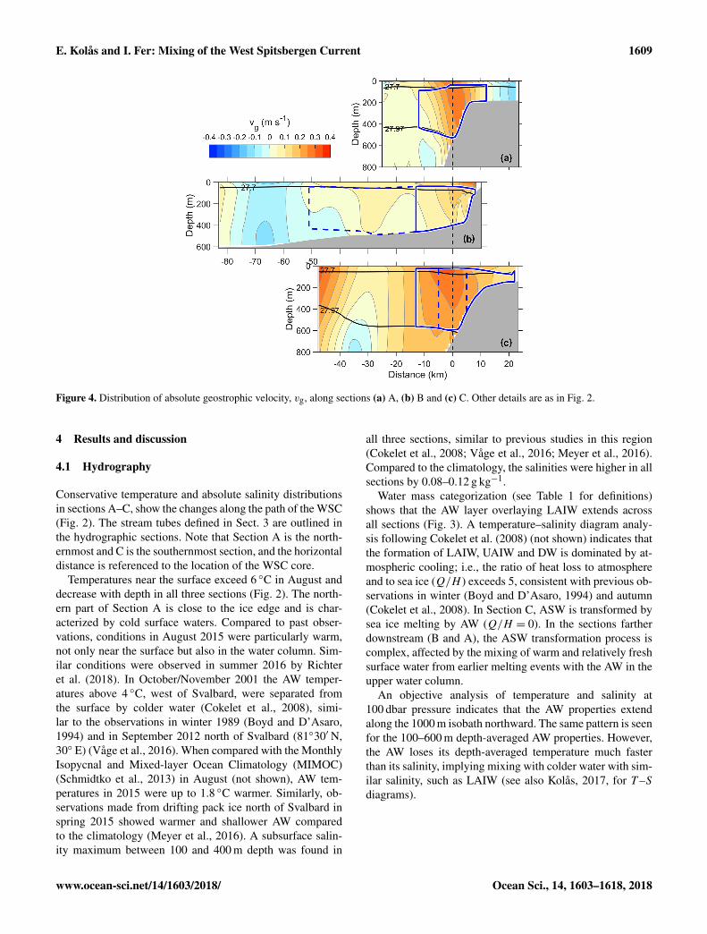
Figure 4. Distribution of absolute geostrophic velocity, vg, along sections (a) A, (b) B and (c) C. Other details are as in Fig. 2.

4 Results and discussion

4.1 Hydrography

Conservative temperature and absolute salinity distributionsin sections A–C, show the changes along the path of the WSC(Fig. 2). The stream tubes defined in Sect. 3 are outlined inthe hydrographic sections. Note that Section A is the north-ernmost and C is the southernmost section, and the horizontaldistance is referenced to the location of the WSC core.

Temperatures near the surface exceed 6 ◦C in August anddecrease with depth in all three sections (Fig. 2). The north-ern part of Section A is close to the ice edge and is char-acterized by cold surface waters. Compared to past obser-vations, conditions in August 2015 were particularly warm,not only near the surface but also in the water column. Sim-ilar conditions were observed in summer 2016 by Richteret al. (2018). In October/November 2001 the AW temper-atures above 4 ◦C, west of Svalbard, were separated fromthe surface by colder water (Cokelet et al., 2008), simi-lar to the observations in winter 1989 (Boyd and D’Asaro,1994) and in September 2012 north of Svalbard (81◦30′ N,30◦ E) (Våge et al., 2016). When compared with the MonthlyIsopycnal and Mixed-layer Ocean Climatology (MIMOC)(Schmidtko et al., 2013) in August (not shown), AW tem-peratures in 2015 were up to 1.8 ◦C warmer. Similarly, ob-servations made from drifting pack ice north of Svalbard inspring 2015 showed warmer and shallower AW comparedto the climatology (Meyer et al., 2016). A subsurface salin-ity maximum between 100 and 400 m depth was found in

all three sections, similar to previous studies in this region(Cokelet et al., 2008; Våge et al., 2016; Meyer et al., 2016).Compared to the climatology, the salinities were higher in allsections by 0.08–0.12 g kg−1.

Water mass categorization (see Table 1 for definitions)shows that the AW layer overlaying LAIW extends acrossall sections (Fig. 3). A temperature–salinity diagram analy-sis following Cokelet et al. (2008) (not shown) indicates thatthe formation of LAIW, UAIW and DW is dominated by at-mospheric cooling; i.e., the ratio of heat loss to atmosphereand to sea ice (Q/H ) exceeds 5, consistent with previous ob-servations in winter (Boyd and D’Asaro, 1994) and autumn(Cokelet et al., 2008). In Section C, ASW is transformed bysea ice melting by AW (Q/H = 0). In the sections fartherdownstream (B and A), the ASW transformation process iscomplex, affected by the mixing of warm and relatively freshsurface water from earlier melting events with the AW in theupper water column.

An objective analysis of temperature and salinity at100 dbar pressure indicates that the AW properties extendalong the 1000 m isobath northward. The same pattern is seenfor the 100–600 m depth-averaged AW properties. However,the AW loses its depth-averaged temperature much fasterthan its salinity, implying mixing with colder water with sim-ilar salinity, such as LAIW (see also Kolås, 2017, for T –Sdiagrams).

www.ocean-sci.net/14/1603/2018/ Ocean Sci., 14, 1603–1618, 2018

1610 E. Kolås and I. Fer: Mixing of the West Spitsbergen Current

4.2 Currents and transport

The spatial distribution of the currents measured by theSADCP helps identify the typical circulation patterns in thestudy region. Objectively interpolated depth-averaged cur-rents from the SADCP show a well-defined Svalbard branchof the WSC along the 400 m isobath (Fig. 1b). The Yer-mak branch however, is not well-captured by the SADCP.If the Yermak branch was present in sections A and C, wewould expect to see evidence of this between x =−5 andx =−15 km. Over the YP, there is no clear evidence ofthe Yermak Pass branch in this snapshot of observations.The absolute geostrophic currents toward the end of Sec-tion B (west of x =−75 km), however, show currents to-ward the Arctic (positive values), which can be a signatureof the Yermak Pass branch. This branch is expected to bevariable and weak in summer (Koenig et al., 2017). Be-tween the Svalbard branch and (possibly) the Yermak Passbranch, a barotropic current is directed southwest, centered atx =−65 km (Fig. 4). North of the Molloy Hole, the currentsare north–northwestward, consistent with the main recircula-tion route for the warmest AW (Hattermann et al., 2016).

The vertical distribution of the observed geostrophic cur-rents along the sections captures the core of the WSC and itslateral extent (Fig. 4). The absolute geostrophic current pro-files show a strong barotropic component. Sections A and Cacross the continental slope have a well-defined WSC corewith a maximum velocity exceeding 0.3 m s−1, typically lo-cated above the 400–600 m isobath. Section B, on the otherhand, extends over the YP.

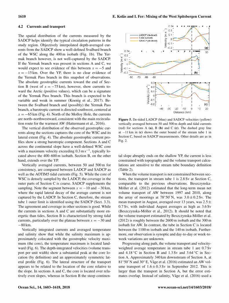
Vertically averaged currents, between 50 and 500 m forconsistency, are compared between LADCP and SADCP aswell as the AOTIM5 tidal currents (Fig. 5). While the core ofWSC is densely sampled by the LADCP, the coverage in theouter parts of Section C is coarse. SADCP supplements thesampling. Note the segment between x =−10 and −30 km,where the rapid lateral decay of the average current is notcaptured by the LADCP. In Section C, therefore, the streamtube 1 outer limit is identified using the SADCP (Sect. 3.3).The agreement and coverage in other sections is good. Whilethe currents in sections A and C are substantially more en-ergetic than tides, Section B is characterized by strong tidalcurrents, particularly over the plateau between x =−30 and−80 km.

Vertically integrated currents and averaged temperatureand salinity show that while the salinity maximum is ap-proximately colocated with the geostrophic velocity maxi-mum (the core), the temperature maximum is located land-ward (Fig. 6). The depth-integrated velocities (volume trans-port per unit width) show a substantial peak at the core lo-cation (by definition) and an approximately symmetric lat-eral profile (Fig. 6). The lateral structure of the transportappears to be related to the location of the core relative tothe slope. In sections A and C, the core is located over rela-tively even slopes, whereas in Section B the steep continen-

Figure 5. De-tided LADCP (blue) and SADCP velocities (yellow)vertically averaged between 50 and 500 m depth and tidal currents(red) for sections A (a), B (b) and C (c). The dashed gray lineat −11 km in (c) shows the outer bound of the stream tube 1 inSection C, based on SADCP measurements. Other details are as inFig. 2.

tal slope abruptly ends on the shallow YP, the current is lessconstrained with topography and the volume transport calcu-lations are sensitive to the stream tube boundary definition(Table 2).

When the volume transport is not constrained between sec-tions, the transport in stream tube 1 is 2.8 Sv at Section C,comparable to the previous observations. Beszczynska-Möller et al. (2012) estimated that the long-term mean netvolume transport of AW between 1997 and 2010, alongthe array of moorings at 78◦50′ N, was 3.0± 0.2 Sv. Themean transport in August, averaged over 13 years, was 2.5±0.7 Sv, with individual August averages as high as 3.6 Sv(Beszczynska-Möller et al., 2012). It should be noted thatthe volume transport estimated by Beszczynska-Möller et al.(2012) is roughly between the 2600 m isobath and the 300 misobath for AW. In contrast, the tube in Section C is locatedbetween the 1100 m isobath and the 140 m isobath. Further-more, our observation is synoptic and day-to-day or week-to-week variations are unknown.

Progressing along path, the volume transport and velocity-weighted average temperature in stream tube 1 are 0.7 Svand 4.18 ◦C in Section B and 1.3 Sv and 3.64 ◦C in Sec-tion A. Approximately 340 km downstream of Section A, at81◦50′ N and 30◦ E, Våge et al. (2016) estimated an AW vol-ume transport of 1.6± 0.3 Sv in September 2012. This islarger than the transport in Section A, but the error esti-mates overlap. Instead of salinity, Våge et al. (2016) used a

Ocean Sci., 14, 1603–1618, 2018 www.ocean-sci.net/14/1603/2018/

E. Kolås and I. Fer: Mixing of the West Spitsbergen Current 1611

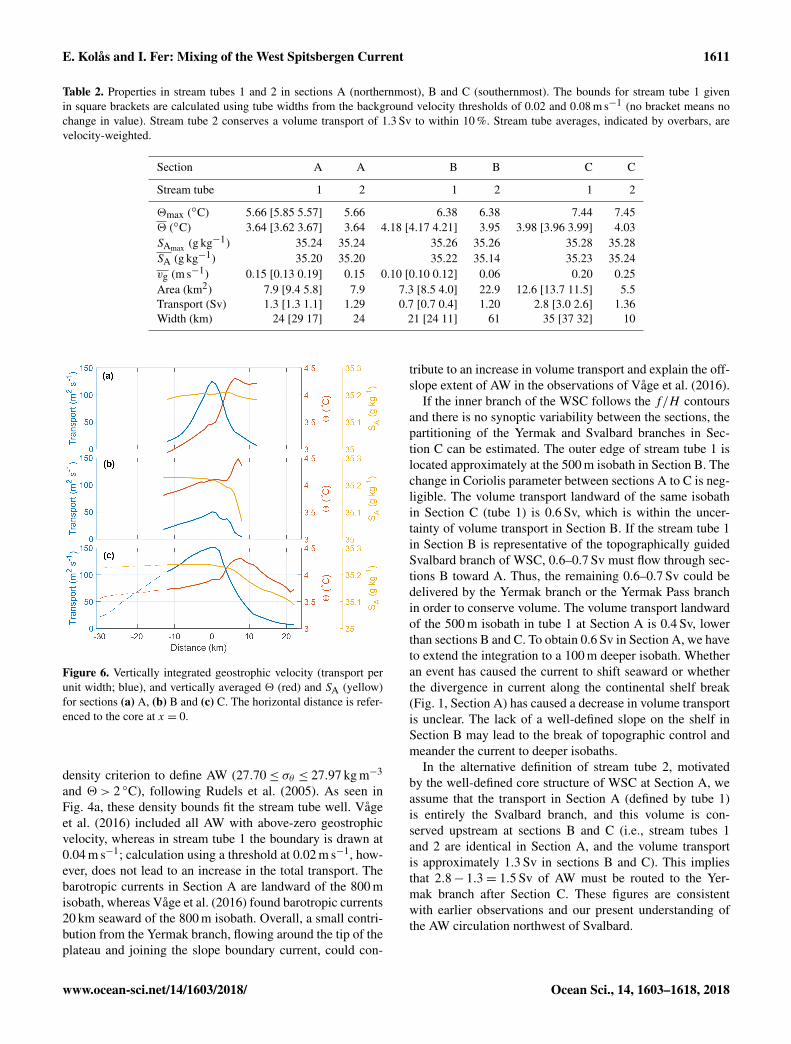
Table 2. Properties in stream tubes 1 and 2 in sections A (northernmost), B and C (southernmost). The bounds for stream tube 1 givenin square brackets are calculated using tube widths from the background velocity thresholds of 0.02 and 0.08 m s−1 (no bracket means nochange in value). Stream tube 2 conserves a volume transport of 1.3 Sv to within 10 %. Stream tube averages, indicated by overbars, arevelocity-weighted.

Section A A B B C C

Stream tube 1 2 1 2 1 2

2max (◦C) 5.66 [5.85 5.57] 5.66 6.38 6.38 7.44 7.452 (◦C) 3.64 [3.62 3.67] 3.64 4.18 [4.17 4.21] 3.95 3.98 [3.96 3.99] 4.03SAmax (g kg−1) 35.24 35.24 35.26 35.26 35.28 35.28SA (g kg−1) 35.20 35.20 35.22 35.14 35.23 35.24vg (m s−1) 0.15 [0.13 0.19] 0.15 0.10 [0.10 0.12] 0.06 0.20 0.25Area (km2) 7.9 [9.4 5.8] 7.9 7.3 [8.5 4.0] 22.9 12.6 [13.7 11.5] 5.5Transport (Sv) 1.3 [1.3 1.1] 1.29 0.7 [0.7 0.4] 1.20 2.8 [3.0 2.6] 1.36Width (km) 24 [29 17] 24 21 [24 11] 61 35 [37 32] 10

Figure 6. Vertically integrated geostrophic velocity (transport perunit width; blue), and vertically averaged 2 (red) and SA (yellow)for sections (a) A, (b) B and (c) C. The horizontal distance is refer-enced to the core at x = 0.

density criterion to define AW (27.70≤ σθ ≤ 27.97 kg m−3

and 2> 2 ◦C), following Rudels et al. (2005). As seen inFig. 4a, these density bounds fit the stream tube well. Vågeet al. (2016) included all AW with above-zero geostrophicvelocity, whereas in stream tube 1 the boundary is drawn at0.04 m s−1; calculation using a threshold at 0.02 m s−1, how-ever, does not lead to an increase in the total transport. Thebarotropic currents in Section A are landward of the 800 misobath, whereas Våge et al. (2016) found barotropic currents20 km seaward of the 800 m isobath. Overall, a small contri-bution from the Yermak branch, flowing around the tip of theplateau and joining the slope boundary current, could con-

tribute to an increase in volume transport and explain the off-slope extent of AW in the observations of Våge et al. (2016).

If the inner branch of the WSC follows the f/H contoursand there is no synoptic variability between the sections, thepartitioning of the Yermak and Svalbard branches in Sec-tion C can be estimated. The outer edge of stream tube 1 islocated approximately at the 500 m isobath in Section B. Thechange in Coriolis parameter between sections A to C is neg-ligible. The volume transport landward of the same isobathin Section C (tube 1) is 0.6 Sv, which is within the uncer-tainty of volume transport in Section B. If the stream tube 1in Section B is representative of the topographically guidedSvalbard branch of WSC, 0.6–0.7 Sv must flow through sec-tions B toward A. Thus, the remaining 0.6–0.7 Sv could bedelivered by the Yermak branch or the Yermak Pass branchin order to conserve volume. The volume transport landwardof the 500 m isobath in tube 1 at Section A is 0.4 Sv, lowerthan sections B and C. To obtain 0.6 Sv in Section A, we haveto extend the integration to a 100 m deeper isobath. Whetheran event has caused the current to shift seaward or whetherthe divergence in current along the continental shelf break(Fig. 1, Section A) has caused a decrease in volume transportis unclear. The lack of a well-defined slope on the shelf inSection B may lead to the break of topographic control andmeander the current to deeper isobaths.

In the alternative definition of stream tube 2, motivatedby the well-defined core structure of WSC at Section A, weassume that the transport in Section A (defined by tube 1)is entirely the Svalbard branch, and this volume is con-served upstream at sections B and C (i.e., stream tubes 1and 2 are identical in Section A, and the volume transportis approximately 1.3 Sv in sections B and C). This impliesthat 2.8− 1.3= 1.5 Sv of AW must be routed to the Yer-mak branch after Section C. These figures are consistentwith earlier observations and our present understanding ofthe AW circulation northwest of Svalbard.

www.ocean-sci.net/14/1603/2018/ Ocean Sci., 14, 1603–1618, 2018

1612 E. Kolås and I. Fer: Mixing of the West Spitsbergen Current

4.3 Cooling and freshening of the WSC

The along-path cooling and freshening of the WSC inferredfrom the change in section-averaged (velocity-weighted)properties from sections C to A are similar to previous ob-servations in summer and fall. The reduction in salinity is0.015 g kg−1/100 km, comparable to the downstream fresh-ening of 0.013/100 km (on the practical salinity scale) re-ported by Cokelet et al. (2008) and the 50-year mean sum-mer freshening of 0.010/100 km, measured by Saloranta andHaugan (2004). The northward temperature gradient corre-sponds to a cooling rate of 0.20 ◦C/100 km for stream tube 1and 0.23 ◦C/100 km for stream tube 2. Cokelet et al. (2008)observed 0.19 ◦C/100 km in fall 2001. Saloranta and Hau-gan (2004) observed a 50-year summer mean cooling rate of0.20 ◦C/100 km, the same as that observed in 1910, between75 and 79◦ N (Helland-Hansen and Nansen, 1912).

Calculation of the northward heat change using Eq. (4)requires the conservation of volume, which is satisfied forstream tube 2 but not in tube 1. In calculations for thetube 1, we use the transport averaged over three sections.The bounds on estimates are obtained from calculations us-ing tube widths from the 0.02 and 0.08 m s−1 backgroundvelocity thresholds (Sect. 3.3), which reflect on velocity-weighted averages, cross section areas, as well as along-path gradients. For tube 1 we obtain an along-path heatchange of −1.3[−1.4, −1.1]× 107 W m−1. When conserv-ing the volume flux at 1.3 Sv, for tube 2, the heat changeis −1.2× 107 W m−1. Dividing by the average tube widthyields an estimate of the surface heat flux, resulting in490 [460 550] W m−2 for tube 1 and 380 W m−2 for tube 2(all rounded to the nearest 10 W m−2).

Boyd and D’Asaro (1994) stated that a winter heat lossper downstream meter of 2× 107 W m−1 (within a factor of2) was needed to cool the warm core as much as observed,comparable to but larger than the cooling rates we observe insummer. For comparison Saloranta and Haugan (2004) esti-mated a summer heat loss of 330 W m−2, and Cokelet et al.(2008) reported 310 W m−2. Both studies used a mean veloc-ity of 0.1 m s−1 when estimating the heat flux. In our obser-vations the mean velocity was 0.15 m s−1; scaling the heatflux in tube 1 by a factor of 1.5 yields a result comparableto that of Saloranta and Haugan (2004) and Cokelet et al.(2008).

An important point to consider when calculating the north-ward cooling rate is the effect of the seasonal temperaturecycle. Using mooring observations in Fram Strait, von Ap-pen et al. (2016) obtain a seasonal signal with temperaturesincreasing from April to September, with an amplitude of2.5 ◦C at 75 m, decreasing to less than 1 ◦C at 250 m depth.The seasonal cycle is likely weaker below 250 m. Our streamtubes span from approximately 50 to 500 m depth. Assumingan average seasonal cycle in our stream tube temperature be-tween 0.5 and 1 ◦C over 5 months (April to September), wecan estimate the northward cooling rate expected from the

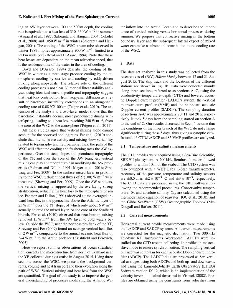
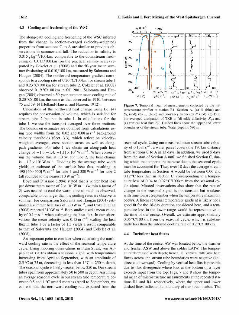
Figure 7. Temporal mean of measurements collected by the mi-crostructure profiler at station R1, Section A. (a) 2 (blue) andSA (red); (b) σθ (blue) and buoyancy frequency N (red); (c) 15 mbin-averaged dissipation of TKE ε; (d) eddy diffusivity Kρ ; and(e) vertical heat flux FH. Dashed lines show the upper and lowerboundaries of the stream tube. Water depth is 690 m.

seasonal cycle. Using our measured mean stream tube veloc-ity of 0.15 m s−1, a water parcel covers the 170 km distancefrom sections C to A in 13 days. In addition, we used 5 daysfrom the start of Section A until we finished Section C, dur-ing which the temperature increase due to the seasonal cyclemust be accounted for. Thus, over 18 days the average streamtube temperature in Section A would be between 0.06 and0.12 ◦C less than in Section C, corresponding to a temper-ature loss of 0.04 to 0.07 ◦C/100 km from the seasonal cy-cle alone. Moored observations also show that the rate ofchange in the seasonal signal is not constant but weakenswith time toward September when the temperature maximumoccurs. A linear seasonal temperature gradient is likely not agood fit for the 18-day duration considered here, and a tem-perature loss in the lower range would be representative atthe time of our cruise. Overall, we estimate approximately0.05 ◦C/100 km from the seasonal cycle, which is substan-tially less than the inferred cooling rate of 0.2 ◦C/100 km.

4.4 Turbulent heat fluxes

At the time of the cruise, AW was located below the warmerand fresher ASW and above the colder LAIW. The temper-ature decreased with depth; hence, all vertical diffusive heatfluxes across the stream tube boundaries were negative (i.e.,directed downward). Cooling by vertical heat flux is possibledue to flux divergence where loss at the bottom of a layerexceeds input from the top. Figs. 7 and 8 show the tempo-ral mean of microstructure measurements at the repeated sta-tions R1 and R4, respectively, where the upper and lowerdashed lines indicate the boundary of our stream tubes. The

Ocean Sci., 14, 1603–1618, 2018 www.ocean-sci.net/14/1603/2018/

E. Kolås and I. Fer: Mixing of the West Spitsbergen Current 1613

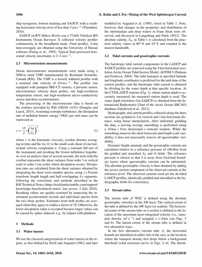
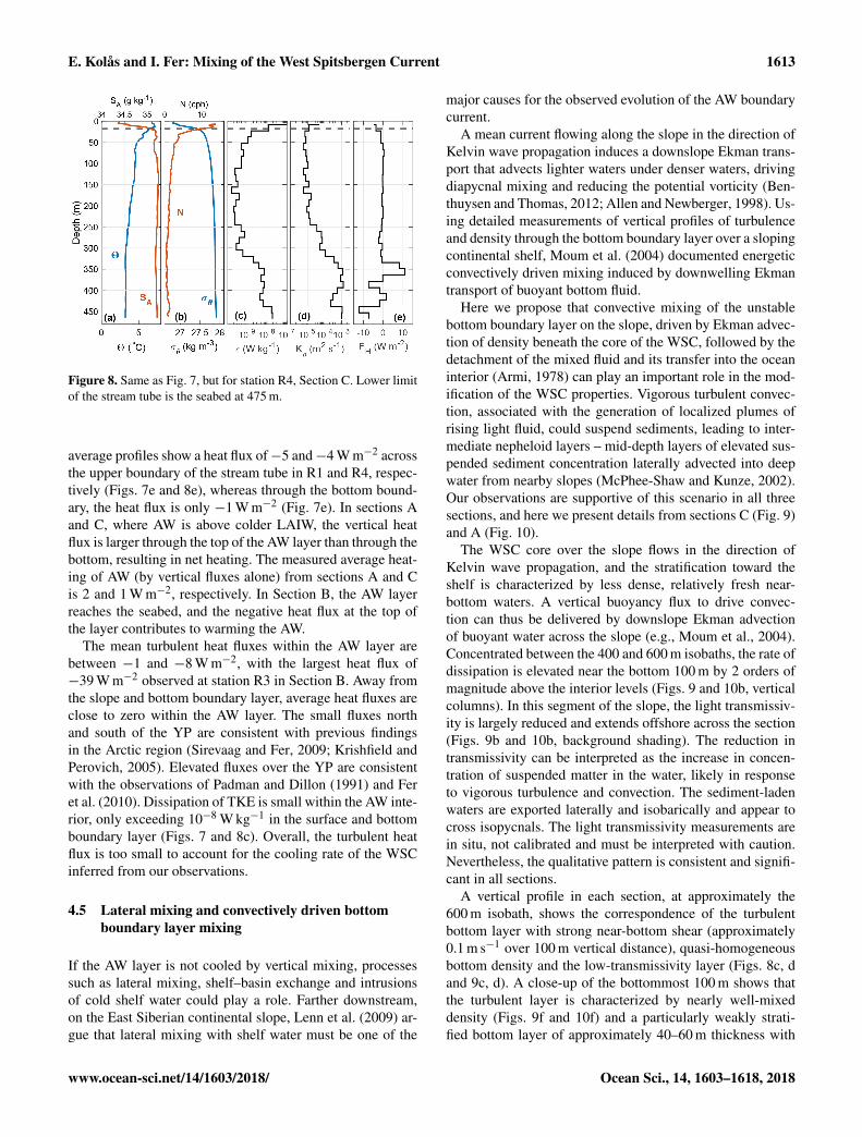
Figure 8. Same as Fig. 7, but for station R4, Section C. Lower limitof the stream tube is the seabed at 475 m.

average profiles show a heat flux of−5 and−4 W m−2 acrossthe upper boundary of the stream tube in R1 and R4, respec-tively (Figs. 7e and 8e), whereas through the bottom bound-ary, the heat flux is only −1 W m−2 (Fig. 7e). In sections Aand C, where AW is above colder LAIW, the vertical heatflux is larger through the top of the AW layer than through thebottom, resulting in net heating. The measured average heat-ing of AW (by vertical fluxes alone) from sections A and Cis 2 and 1 W m−2, respectively. In Section B, the AW layerreaches the seabed, and the negative heat flux at the top ofthe layer contributes to warming the AW.

The mean turbulent heat fluxes within the AW layer arebetween −1 and −8 W m−2, with the largest heat flux of−39 W m−2 observed at station R3 in Section B. Away fromthe slope and bottom boundary layer, average heat fluxes areclose to zero within the AW layer. The small fluxes northand south of the YP are consistent with previous findingsin the Arctic region (Sirevaag and Fer, 2009; Krishfield andPerovich, 2005). Elevated fluxes over the YP are consistentwith the observations of Padman and Dillon (1991) and Feret al. (2010). Dissipation of TKE is small within the AW inte-rior, only exceeding 10−8 W kg−1 in the surface and bottomboundary layer (Figs. 7 and 8c). Overall, the turbulent heatflux is too small to account for the cooling rate of the WSCinferred from our observations.

4.5 Lateral mixing and convectively driven bottomboundary layer mixing

If the AW layer is not cooled by vertical mixing, processessuch as lateral mixing, shelf–basin exchange and intrusionsof cold shelf water could play a role. Farther downstream,on the East Siberian continental slope, Lenn et al. (2009) ar-gue that lateral mixing with shelf water must be one of the

major causes for the observed evolution of the AW boundarycurrent.

A mean current flowing along the slope in the direction ofKelvin wave propagation induces a downslope Ekman trans-port that advects lighter waters under denser waters, drivingdiapycnal mixing and reducing the potential vorticity (Ben-thuysen and Thomas, 2012; Allen and Newberger, 1998). Us-ing detailed measurements of vertical profiles of turbulenceand density through the bottom boundary layer over a slopingcontinental shelf, Moum et al. (2004) documented energeticconvectively driven mixing induced by downwelling Ekmantransport of buoyant bottom fluid.

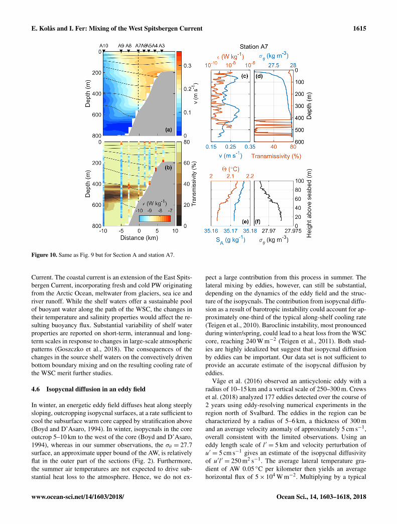
Here we propose that convective mixing of the unstablebottom boundary layer on the slope, driven by Ekman advec-tion of density beneath the core of the WSC, followed by thedetachment of the mixed fluid and its transfer into the oceaninterior (Armi, 1978) can play an important role in the mod-ification of the WSC properties. Vigorous turbulent convec-tion, associated with the generation of localized plumes ofrising light fluid, could suspend sediments, leading to inter-mediate nepheloid layers – mid-depth layers of elevated sus-pended sediment concentration laterally advected into deepwater from nearby slopes (McPhee-Shaw and Kunze, 2002).Our observations are supportive of this scenario in all threesections, and here we present details from sections C (Fig. 9)and A (Fig. 10).

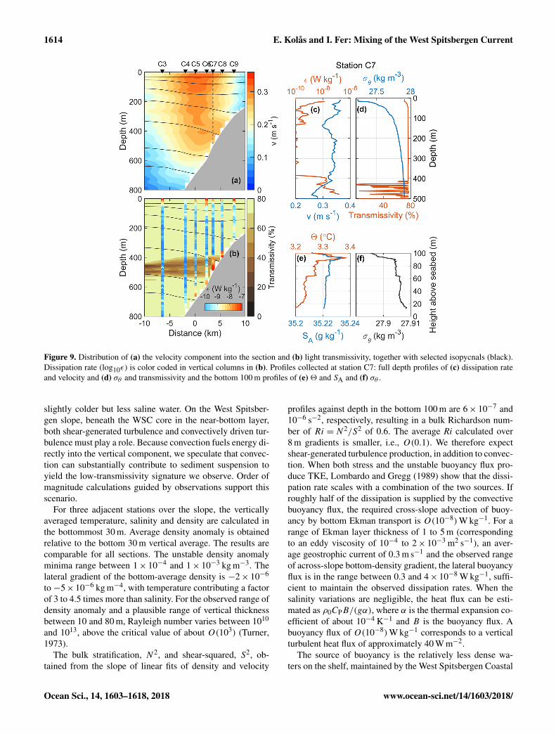
The WSC core over the slope flows in the direction ofKelvin wave propagation, and the stratification toward theshelf is characterized by less dense, relatively fresh near-bottom waters. A vertical buoyancy flux to drive convec-tion can thus be delivered by downslope Ekman advectionof buoyant water across the slope (e.g., Moum et al., 2004).Concentrated between the 400 and 600 m isobaths, the rate ofdissipation is elevated near the bottom 100 m by 2 orders ofmagnitude above the interior levels (Figs. 9 and 10b, verticalcolumns). In this segment of the slope, the light transmissiv-ity is largely reduced and extends offshore across the section(Figs. 9b and 10b, background shading). The reduction intransmissivity can be interpreted as the increase in concen-tration of suspended matter in the water, likely in responseto vigorous turbulence and convection. The sediment-ladenwaters are exported laterally and isobarically and appear tocross isopycnals. The light transmissivity measurements arein situ, not calibrated and must be interpreted with caution.Nevertheless, the qualitative pattern is consistent and signifi-cant in all sections.

A vertical profile in each section, at approximately the600 m isobath, shows the correspondence of the turbulentbottom layer with strong near-bottom shear (approximately0.1 m s−1 over 100 m vertical distance), quasi-homogeneousbottom density and the low-transmissivity layer (Figs. 8c, dand 9c, d). A close-up of the bottommost 100 m shows thatthe turbulent layer is characterized by nearly well-mixeddensity (Figs. 9f and 10f) and a particularly weakly strati-fied bottom layer of approximately 40–60 m thickness with

www.ocean-sci.net/14/1603/2018/ Ocean Sci., 14, 1603–1618, 2018

1614 E. Kolås and I. Fer: Mixing of the West Spitsbergen Current

Figure 9. Distribution of (a) the velocity component into the section and (b) light transmissivity, together with selected isopycnals (black).Dissipation rate (log10ε) is color coded in vertical columns in (b). Profiles collected at station C7: full depth profiles of (c) dissipation rateand velocity and (d) σθ and transmissivity and the bottom 100 m profiles of (e) 2 and SA and (f) σθ .

slightly colder but less saline water. On the West Spitsber-gen slope, beneath the WSC core in the near-bottom layer,both shear-generated turbulence and convectively driven tur-bulence must play a role. Because convection fuels energy di-rectly into the vertical component, we speculate that convec-tion can substantially contribute to sediment suspension toyield the low-transmissivity signature we observe. Order ofmagnitude calculations guided by observations support thisscenario.

For three adjacent stations over the slope, the verticallyaveraged temperature, salinity and density are calculated inthe bottommost 30 m. Average density anomaly is obtainedrelative to the bottom 30 m vertical average. The results arecomparable for all sections. The unstable density anomalyminima range between 1× 10−4 and 1× 10−3 kg m−3. Thelateral gradient of the bottom-average density is −2× 10−6

to −5×10−6 kg m−4, with temperature contributing a factorof 3 to 4.5 times more than salinity. For the observed range ofdensity anomaly and a plausible range of vertical thicknessbetween 10 and 80 m, Rayleigh number varies between 1010

and 1013, above the critical value of about O(103) (Turner,1973).

The bulk stratification, N2, and shear-squared, S2, ob-tained from the slope of linear fits of density and velocity

profiles against depth in the bottom 100 m are 6× 10−7 and10−6 s−2, respectively, resulting in a bulk Richardson num-ber of Ri =N2/S2 of 0.6. The average Ri calculated over8 m gradients is smaller, i.e., O(0.1). We therefore expectshear-generated turbulence production, in addition to convec-tion. When both stress and the unstable buoyancy flux pro-duce TKE, Lombardo and Gregg (1989) show that the dissi-pation rate scales with a combination of the two sources. Ifroughly half of the dissipation is supplied by the convectivebuoyancy flux, the required cross-slope advection of buoy-ancy by bottom Ekman transport is O(10−8)W kg−1. For arange of Ekman layer thickness of 1 to 5 m (correspondingto an eddy viscosity of 10−4 to 2× 10−3 m2 s−1), an aver-age geostrophic current of 0.3 m s−1 and the observed rangeof across-slope bottom-density gradient, the lateral buoyancyflux is in the range between 0.3 and 4× 10−8 W kg−1, suffi-cient to maintain the observed dissipation rates. When thesalinity variations are negligible, the heat flux can be esti-mated as ρ0CPB/(gα), where α is the thermal expansion co-efficient of about 10−4 K−1 and B is the buoyancy flux. Abuoyancy flux of O(10−8)W kg−1 corresponds to a verticalturbulent heat flux of approximately 40 W m−2.

The source of buoyancy is the relatively less dense wa-ters on the shelf, maintained by the West Spitsbergen Coastal

Ocean Sci., 14, 1603–1618, 2018 www.ocean-sci.net/14/1603/2018/

E. Kolås and I. Fer: Mixing of the West Spitsbergen Current 1615

Figure 10. Same as Fig. 9 but for Section A and station A7.

Current. The coastal current is an extension of the East Spits-bergen Current, incorporating fresh and cold PW originatingfrom the Arctic Ocean, meltwater from glaciers, sea ice andriver runoff. While the shelf waters offer a sustainable poolof buoyant water along the path of the WSC, the changes intheir temperature and salinity properties would affect the re-sulting buoyancy flux. Substantial variability of shelf waterproperties are reported on short-term, interannual and long-term scales in response to changes in large-scale atmosphericpatterns (Goszczko et al., 2018). The consequences of thechanges in the source shelf waters on the convectively drivenbottom boundary mixing and on the resulting cooling rate ofthe WSC merit further studies.

4.6 Isopycnal diffusion in an eddy field

In winter, an energetic eddy field diffuses heat along steeplysloping, outcropping isopycnal surfaces, at a rate sufficient tocool the subsurface warm core capped by stratification above(Boyd and D’Asaro, 1994). In winter, isopycnals in the coreoutcrop 5–10 km to the west of the core (Boyd and D’Asaro,1994), whereas in our summer observations, the σθ = 27.7surface, an approximate upper bound of the AW, is relativelyflat in the outer part of the sections (Fig. 2). Furthermore,the summer air temperatures are not expected to drive sub-stantial heat loss to the atmosphere. Hence, we do not ex-

pect a large contribution from this process in summer. Thelateral mixing by eddies, however, can still be substantial,depending on the dynamics of the eddy field and the struc-ture of the isopycnals. The contribution from isopycnal diffu-sion as a result of barotropic instability could account for ap-proximately one-third of the typical along-shelf cooling rate(Teigen et al., 2010). Baroclinic instability, most pronouncedduring winter/spring, could lead to a heat loss from the WSCcore, reaching 240 W m−2 (Teigen et al., 2011). Both stud-ies are highly idealized but suggest that isopycnal diffusionby eddies can be important. Our data set is not sufficient toprovide an accurate estimate of the isopycnal diffusion byeddies.

Våge et al. (2016) observed an anticyclonic eddy with aradius of 10–15 km and a vertical scale of 250–300 m. Crewset al. (2018) analyzed 177 eddies detected over the course of2 years using eddy-resolving numerical experiments in theregion north of Svalbard. The eddies in the region can becharacterized by a radius of 5–6 km, a thickness of 300 mand an average velocity anomaly of approximately 5 cm s−1,overall consistent with the limited observations. Using aneddy length scale of l′ = 5 km and velocity perturbation ofu′ = 5 cm s−1 gives an estimate of the isopycnal diffusivityof u′l′ = 250 m2 s−1. The average lateral temperature gra-dient of AW 0.05 ◦C per kilometer then yields an averagehorizontal flux of 5× 104 W m−2. Multiplying by a typical

www.ocean-sci.net/14/1603/2018/ Ocean Sci., 14, 1603–1618, 2018

1616 E. Kolås and I. Fer: Mixing of the West Spitsbergen Current

eddy thickness of 300 m, we obtain (1− 2)× 107 W m−1,lost laterally outward along the side of the stream tube. Thisis of the same order as the estimated along-path heat change.Assuming a fraction (0.5) of the along-path distance is af-fected by eddies will result in half of the heat loss unex-plained, unaccounted for by interior diapycnal mixing andeddy-induced isopycnal diffusion. The cooling induced byconvectively driven bottom mixing can thus be important.

5 Conclusions

Observations from a cruise conducted in August 2015 pro-vide a snapshot of the West Spitsbergen Current (WSC) hy-drography, transport and mixing in ice-free regions west andnorth of Svalbard in a year with relatively warmer and saltierAtlantic Water (AW) compared to climatology. Data werecollected in three sections across the WSC, along an approx-imately 170 km long path.

The Svalbard branch of the WSC is topographicallyguided close to the shelf break and is relatively well capturedby our observations. The recirculating branch in Fram Strait,the Yermak branch and the Yermak Pass branch are not re-solved, but inferences are made from the observed sections.The volume transport in a stream tube of WSC, defined usingthe AW properties and along-path velocities above a back-ground value, is 2.8 Sv in Fram Strait before the Svalbardand Yermak branches split. The transport reduces to 1.3 Sv inthe most downstream section north of Svalbard. In a scenariowhere the Svalbard branch is constrained to the 500 m iso-bath in the middle section, its volume transport is 0.6–0.7 Sv,implying that approximately 2 Sv is fed to recirculation andYermak branch in Fram Strait, and 0.6–0.7 Sv is potentiallydelivered by the Yermak branch or the Yermak Pass branchwhich could join the Svalbard branch in the northern section.An alternative scenario, assuming the transport in the mostdownstream section is entirely the Svalbard branch (1.3 Sv)and this volume is conserved in the sections upstream, im-plies that 1.5 Sv of AW must be routed to the Yermak Branchin Fram Strait.

The along-path cooling of the WSC is similar to previousobservations in summer and fall, with approximately 0.20 ◦Cper 100 km. The associated bulk heat loss per along-path me-ter is (1.1− 1.4)× 107 W m−1, corresponding to a surfaceheat flux of 380–550 W m−2. The measured turbulent heatflux is too small to account for this cooling rate. In contrastto winter conditions, we do not expect heat loss by diffusionalong outcropping isopycnals. The lateral mixing by eddies,however, can be substantial, depending on the dynamics ofthe eddy field and the structure of the isopycnals. While ourobservations are not sufficient to allow an accurate quantifi-cation of the diffusion by eddies, estimates using a plausiblerange of parameters suggest that the contribution from ed-dies could be limited to one half of the observed heat loss.We propose that energetic convective mixing of the unstable

bottom boundary layer on the slope, driven by Ekman advec-tion of density beneath the core of the WSC, followed by thedetachment of the mixed fluid and its transfer into the oceaninterior can explain a significant part of the remaining heatloss.

The WSC core on the slope flows in the direction ofKelvin wave propagation, inducing the downslope Ekmanadvection. Relatively less dense near-bottom waters on theshelf are the source of buoyancy, maintained by the coldand fresh waters from the Svalbard coast and fjords join-ing the west Spitsbergen coastal current. Our detailed ob-servations show turbulence generation through a combina-tion of mean shear and convection. Downslope Ekman ad-vection across the slope leads to a lateral buoyancy flux ofO(10−8)W kg−1, sufficient to maintain a large fraction ofthe observed dissipation rates, and corresponds to a heat fluxof approximately 40 W m2. Convectively driven bottom mix-ing can be important for cooling and freshening of the WSC.

Data availability. The data set is available through the NorwegianMarine Data Centre: https://doi.org/10.21335/NMDC-567625440(Fer and Kolås, 2018).

Author contributions. IF designed the experiment; EK and IF col-lected the data, conceived and planned the analysis. EK performedthe analysis and wrote the paper, with advice and critical feedbackfrom IF. Both authors discussed the results and finalized the paper.

Competing interests. The authors declare that they have no conflictof interest.

Acknowledgements. This study was supported by the ResearchCouncil of Norway through the project 229786. The work is basedon the MSc study of Eivind Kolås (Kolås, 2017). We thank thecrew and participants of the cruise HM 2015617. We also thankIgor Polyakov and an anonymous reviewer for their valuablecomments that helped improve an earlier version of the paper.

Edited by: Matthew HechtReviewed by: Igor Polyakov and one anonymous referee

References

Aagaard, K., Swift, J. H., and Carmack, E. C.: Thermohaline cir-culation in the Arctic Mediterranean Seas, J. Geophys. Res., 90,4833, https://doi.org/10.1029/JC090iC03p04833, 1985.

Aagaard, K., Foldvik, A., and Hillman, S. R.: The West SpitsbergenCurrent: Disposition and water mass transformation, J. Geophys.Res., 92, 3778–3784, https://doi.org/10.1029/JC092iC04p03778,1987.

Allen, J. S. and Newberger, P. A.: On Symmetric Insta-bilities in Oceanic Bottom Boundary Layers, J. Phys.

Ocean Sci., 14, 1603–1618, 2018 www.ocean-sci.net/14/1603/2018/

E. Kolås and I. Fer: Mixing of the West Spitsbergen Current 1617

Oceanogr., 28, 1131–1151, https://doi.org/10.1175/1520-0485(1998)028<1131:osiiob>2.0.co;2, 1998.

Armi, L.: Some evidence for boundary mixing in the deep ocean, J.Geophys. Res., 83, 1971–1979, 1978.

Benthuysen, J. and Thomas, L. N.: Friction and Diapycnal Mix-ing at a Slope: Boundary Control of Potential Vorticity, J.Phys. Oceanogr., 42, 1509–1523, https://doi.org/10.1175/jpo-d-11-0130.1, 2012.

Beszczynska-Möller, A., Fahrbach, E., Schauer, U., and Hansen, E.:Variability in Atlantic water temperature and transport at the en-trance to the Arctic Ocean, 1997–2010, ICES J. Mar. Sci., 69,852–863, https://doi.org/10.1093/icesjms/fss056, 2012.

Böhme, L. and Send, U.: Objective analyses of hydrographic datafor referencing profiling float salinities in highly variable envi-ronments, Deep-Sea Res. Pt. II, 52, 651–664, 2005.

Boyd, T. J. and D’Asaro, E. A.: Cooling of the West SpitsbergenCurrent: Wintertime Observations West of Svalbard, J. Geophys.Res., 99, 22597–22618, https://doi.org/10.1029/94JC01824,1994.

Cokelet, E. D., Tervalon, N., and Bellingham, J. G.: Hy-drography of the West Spitsbergen Current, SvalbardBranch: Autumn 2001, J. Geophys. Res., 113, C01006,https://doi.org/10.1029/2007JC004150, 2008.

Crews, L., Sundfjord, A., Albretsen, J., and Hattermann, T.:Mesoscale Eddy Activity and Transport in the Atlantic Water In-flow Region North of Svalbard, J. Geophys. Res., 123, 201–215,2018.

Douglas, W. and Lueck, R.: ODAS MATLAB Library. TechnicalManual, Version 4.0, Tech. rep., Rockland Scientific Interna-tional Inc., available at: https://rocklandscientific.com (last ac-cess: 2 July 2018), 2015.

Fahrbach, E., Meincke, J., Østerhus, S., Rohardt, G., Schauer,U., Tverberg, V., Verduin, J., and Woodgate, R. A.: Directmeasurements of heat and mass transports through the FramStrait, Polar Res., 20, 217–224, https://doi.org/10.1111/j.1751-8369.2001.tb00059.x, 2001.

Farrelly, B., Gammelsrød, T., Golmen, L. G., and Sjøberg, B.:Hydrographic conditions in the Fram Strait, summer 1982,Polar Res., 3, 227–238, https://doi.org/10.1111/j.1751-8369.1985.tb00509.x, 1985.

Fer, I. and Kolås, E.: Ocean currents, hydrography and microstruc-ture data from cruise HM2015617, Norwegian Marine Data Cen-tre, https://doi.org/10.21335/NMDC-567625440, 2018.

Fer, I., Skogseth, R., and Geyer, F.: Internal waves and mixing in theMarginal Ice Zone near the Yermak Plateau, J. Phys. Oceanogr.,40, 1613–1630, https://doi.org/10.1175/2010JPO4371.1, 2010.

Firing, E., Ranada, J., and Caldwell, P.: Processing ADCP data withthe CODAS software system version 3.1, Joint Institute for Ma-rine and Atmospheric Research, University of Hawaii & NationalOceanographic Data Center, PANGAEA, Bremerhaven, p. 226,1995.

Gascard, J. C., Richez, C., and Roaualt, C.: New insights on large-scale oceanography in Fram Strait: the West Spitsbergen Cur-rent, in: Arctic oceanography, marginal ice zones and continentalshelves, vol. 49, chap. 5, edited by: Smith Jr., W. O. and Greb-meier, J., AGU, Washington, D.C., 131–182, 1995.

Goszczko, I., Ingvaldsen, R. B., and Onarheim, I. H.: Wind-Driven Cross-Shelf Exchange – West Spitsbergen Currentas a Source of Heat and Salt for the Adjacent Shelf in

Arctic Winters, J. Geophys. Res.-Oceans, 123, 2668–2696,https://doi.org/10.1002/2017JC013553, 2018.

Gregg, M., D’Asaro, E., Riley, J., and Kunze, E.: Mixing Ef-ficiency in the Ocean, Annu. Rev. Mar. Sci., 10, 443–473,https://doi.org/10.1146/annurev-marine-121916-063643, 2018.

Hattermann, T., Isachsen, P. E., Von Appen, W. J., Albretsen,J., and Sundfjord, A.: Eddy-driven recirculation of AtlanticWater in Fram Strait, Geophys. Res. Lett., 43, 3406–3414,https://doi.org/10.1002/2016GL068323, 2016.

Helland-Hansen, B. and Nansen, F.: The Sea West of Spitsber-gen, The Oceanographic Observations of the Isachsen Spitsber-gen Expedition in 1910, Vetenskapsselskpaets Skrifter. I. Mat.-Maturv. Klasse, 12, 89, 1912.

IOC, SCOR, and IAPSO: The international thermodynamic equa-tion of seawater – 2010: Calculations and use of thermody-namic properties, Intergovernmental Oceanographic Commis-sion, Manuals and Guides No. 56, Tech. rep., UNESCO, 196 pp.,2010.

Jakobsson, M., Mayer, L., Coakley, B., Dowdeswell, J. A., Forbes,S., Fridman, B., Hodnesdal, H., Noormets, R., Pedersen, R.,Rebesco, M., Schenke, H. W., Zarayskaya, Y., Accettella, D.,Armstrong, A., Anderson, R. M., Beinhoff, P., Camerlenghi, A.,Church, I., Edwards, M., Gerdner, J. V., Hall, J. K., Hell, B.,Hestvik, O., Kristoffersen, Y., Marcussen, C., Mohammad, R.,Mosher, D., Ngheim, S. V., Pedrosa, M. T., Travaglini, P. G., andWeatherall, P.: The International Bathymetric Chart of the ArcticOcean (IBCAO) Version 3.0, Geophys. Res. Lett., 39, L12609,https://doi.org/10.1029/2012GL052219, 2012.

Koenig, Z., Provost, C., Sennéchael, N., Garric, G., and Gascard, J.C.: The Yermak Pass Branch: A Major Pathway for the AtlanticWater North of Svalbard?, J. Geophys. Res., 122, 9332–9349,https://doi.org/10.1002/2017JC013271, 2017.

Kolås, E.: The Svalbard branch of the West Spitsbergen Current:Hydrography, transport and mixing, MS thesis, University ofBergen, Bergen, available at: http://hdl.handle.net/1956/16389(last access: 2 July 2018), 2017.

Krishfield, R. A. and Perovich, D. K.: Spatial and temporal variabil-ity of oceanic heat flux to the Arctic ice pack, J. Geophys. Res.,110, 1–20, https://doi.org/10.1029/2004JC002293, 2005.

Langehaug, H. R. and Falck, E.: Changes in the proper-ties and distribution of the intermediate and deep wa-ters in the Fram Strait, Prog. Oceanogr., 96, 57–76,https://doi.org/10.1016/j.pocean.2011.10.002, 2012.

Lenn, Y. D., Wiles, P. J., Torres-Valdes, S., Abrahamsen, E. P., Rip-peth, T. P., Simpson, J. H., Bacon, S., Laxon, S. W., Polyakov,I., Ivanov, V., and Kirillov, S.: Vertical mixing at intermediatedepths in the Arctic boundary current, Geophys. Res. Lett., 36,L05601, https://doi.org/10.1029/2008GL036792, 2009.

Lombardo, C. P. and Gregg, M. C.: Similarity scaling of viscous andthermal dissipation in a convecting boundary layer, J. Geophys.Res., 94, 6273–6284, 1989.

McDougall, T. J. and Barker, P. M.: Getting started with TEOS-10 and the Gibbs Seawater (GSW) Oceanographic Toolbox,SCOR/IAPSO WG127, 28 pp., 2011.

McPhee-Shaw, E. E. and Kunze, E.: Boundary layer intru-sions from a sloping bottom: A mechanism for generatingintermediate nepheloid layers, J. Geophys. Res., 107, 3050,https://doi.org/10.1029/2001jc000801, 2002.

www.ocean-sci.net/14/1603/2018/ Ocean Sci., 14, 1603–1618, 2018

1618 E. Kolås and I. Fer: Mixing of the West Spitsbergen Current

Meyer, A., Sundfjord, A., Fer, I., Provost, C., Vilacieros-Robineau,N., Koenig, Z., Onarheim, I. H., Smedsrud, L. H., Duarte, P.,Dodd, P. A., Graham, R. M., Schmidtko, S., and Kauko, H. M.:Winter to summer hydrographic and current observations in theArctic Ocean north of Svalbard, J. Geophys. Res., 122, 1–49,https://doi.org/10.1002/2016JC012391, 2016.

Moum, J. N., Perlin, A., Klymak, J. M., Levine, M. D., Boyd, T., andKosro, P. M.: Convectively driven mixing in the bottom boundarylayer, J. Phys. Oceanogr., 34, 2189–2202, 2004.

Osborn, T. R.: Estimates of the local rate of vertical diffusion fromdissipation measurements, J. Phys. Oceanogr., 10, 83–89, 1980.

Padman, L. and Dillon, T. M.: Turbulent mixing nearthe Yermak Plateau during the Coordinated EasternArctic Experiment, J. Geophys. Res., 96, 4769–4782,https://doi.org/10.1029/90JC02260, 1991.

Padman, L. and Erofeeva, S.: A barotropic inverse tidal modelfor the Arctic Ocean, Geophys. Res. Lett., 31, L02303,https://doi.org/10.1029/2003GL019003, 2004.

Perkin, R. G. and Lewis, E. L.: Mixing in theWest Spitsbergen Current, J. Phys. Oceanogr.,14, 1315–1325, https://doi.org/10.1175/1520-0485(1984)014<1315:MITWSC>2.0.CO;2, 1984.

Pnyushkov, A. V., Polyakov, I. V., Ivanov, V. V., Aksenov, Y.,Coward, A. C., Janout, M., and Rabe, B.: Structure andvariability of the boundary current in the Eurasian Basinof the Arctic Ocean, Deep-Sea Res. Pt. I, 101, 80–97,https://doi.org/10.1016/j.dsr.2015.03.001, 2015.

Polyakov, I. V., Pnyushkov, A. V., Alkire, M. B., Ashik, I. M., Bau-mann, T. M., Carmack, E. C., Goszczko, I., Guthrie, J., Ivanov, V.V., Kanzow, T., Krishfield, R., Kwok, R., Sundfjord, A., Morison,J., Rember, R., and Yulin, A.: Greater role for Atlantic inflows onsea-ice loss in the Eurasian Basin of the Arctic Ocean, Science,356, 285–291, https://doi.org/10.1126/science.aai8204, 2017.

Richter, M. E., von Appen, W.-J., and Wekerle, C.: Does the EastGreenland Current exist in the northern Fram Strait?, Ocean Sci-ence, 14, 1147–1165, https://doi.org/10.5194/os-14-1147-2018,2018.

Rudels, B., Björk, G., Nilsson, J., Winsor, P., Lake, I., andNohr, C.: The interaction between waters from the Arc-tic Ocean and the Nordic Seas north of Fram Strait andalong the East Greenland Current: results from the Arc-tic Ocean-O2 Oden expedition, J. Mar. Syst., 55, 1–30,https://doi.org/10.1016/j.jmarsys.2004.06.008, 2005.

Rudels, B., Korhonen, M., Schauer, U., Pisarev, S., Rabe, B., andWisotzki, A.: Circulation and transformation of Atlantic water inthe Eurasian Basin and the contribution of the Fram Strait inflowbranch to the Arctic Ocean heat budget, Prog. Oceanogr., 132,128–152, https://doi.org/10.1016/j.pocean.2014.04.003, 2015.

Saloranta, T. M. and Haugan, P. M.: Northward cooling and freshen-ing of the warm core of the West Spitsbergen Current, Polar Res.,23, 79–88, https://doi.org/10.1111/j.1751-8369.2004.tb00131.x,2004.

Schauer, U., Fahrbach, E., Østerhus, S., and Rohardt, G.: Arc-tic warming through the Fram Strait: Oceanic heat transportfrom 3 years of measurements, J. Geophys. Res., 109, C06026,https://doi.org/10.1029/2003JC001823, 2004.

Schmidtko, S., Johnson, G. C., and Lyman, J. M.: MI-MOC: A global monthly isopycnal upper-ocean climatol-ogy with mixed layers, J. Geophys. Res., 118, 1658–1672,https://doi.org/10.1002/jgrc.20122, 2013.

Sirevaag, A. and Fer, I.: Early Spring Oceanic HeatFluxes and Mixing Observed from Drift StationsNorth of Svalbard, J. Phys. Oceanogr., 39, 3049–3069,https://doi.org/10.1175/2009JPO4172.1, 2009.

Swift, J. H. and Aagaard, K.: Seasonal transitions and watermass formation in the Iceland and Greenland seas, Deep-Sea Res. Pt. A, 28, 1107–1129, https://doi.org/10.1016/0198-0149(81)90050-9, 1981.

Teigen, S. H., Nilsen, F., and Gjevik, B.: Barotropic instability inthe West Spitsbergen Current, J. Geophys. Res., 115, C07016,https://doi.org/10.1029/2009JC005996, 2010.

Teigen, S. H., Nilsen, F., Skogseth, R., Gjevik, B., andBeszczynska-Möller, A.: Baroclinic instability in theWest Spitsbergen Current, J. Geophys. Res., 116, C07012,https://doi.org/10.1029/2011JC006974, 2011.

Thurnherr, A. M.: A Practical Assessment of the ErrorsAssociated with Full-Depth LADCP Profiles ObtainedUsing Teledyne RDI Workhorse Acoustic Doppler Cur-rent Profilers, J. Atmos. Ocean. Tech., 27, 1215–1227,https://doi.org/10.1175/2010JTECHO708.1, 2010.

Turner, J. S.: Buoyancy Effects in Fluids, Cambridge UniversityPress, New York, 1973.

Våge, K., Pickart, R. S., Pavlov, V., Lin, P., Torres, D. J., Ingvald-sen, R., Sundfjord, A., and Proshutinsky, A.: The Atlantic Wa-ter boundary current in the Nansen Basin: Transport and mech-anisms of lateral exchange, J. Geophys. Res., 121, 6946–6960,https://doi.org/10.1002/2016JC011715, 2016.

Visbeck, M.: Deep velocity profiling using low-ered acoustic Doppler current profilers: Bottomtrack and inverse solutions, J. Atmos. Ocean.Tech., 19, 794–807, https://doi.org/10.1175/1520-0426(2002)019<0794:DVPULA>2.0.CO;2, 2002.

von Appen, W.-J., Schauer, U., Hattermann, T., and Beszczynska-Möller, A.: Seasonal Cycle of Mesoscale Instability of theWest Spitsbergen Current, J. Phys. Oceanogr., 46, 1231–1254,https://doi.org/10.1175/JPO-D-15-0184.1, 2016.

Ocean Sci., 14, 1603–1618, 2018 www.ocean-sci.net/14/1603/2018/