Embed Size (px)
Citation preview
NOVA Technical Note 5
1 | P a g e
Autolab SDK
Case study: using the Autolab SDK to develop NOVA applications in LabVIEW
1 – What is the Autolab SDK?
The Autolab Software Development Kit (Autolab SDK) is designed to control the Autolab instrument from different external applications such as LabVIEW, Visual Basic for Applications (VBA), scripting, etc. With the Autolab SDK the external application can be used to measure complete procedures or control individual Autolab modules.
The most common application of the Autolab SDK is the combination with LabVIEW. For this purpose, the Autolab SDK comes with a number of pre-defined LabVIEW examples (called VIs – for Virtual Instrument). These basic examples can be used to illustrate the control of the Autolab in LabVIEW.
This technical note provides more information on the use of the Autolab SDK in combination with LabVIEW. Two Vis, installed with the Autolab SDK, are illustrated in this note.
2 – Loading the new Autolab LabVIEW project
Once the files have been extracted from the zip file, open the C:\Program Files\Metrohm Autolab\Autolab SDK 1.10 folder and simply double-click the Autolab.lvproj file to start LabVIEW and load this project.
Note
The VIs provided with the Autolab SDK require LabVIEW 2010 or later. The Autolab SDK must be installed on the computer. Nova does not have to be installed on the computer since the Autolab SDK can be used as a stand-alone application.
Warning
A special configuration file is required in order to support the .NET 4.0 frame-work support in LabVIEW 2010 and later. A knowledge base article is available here: http://digital.ni.com/public.nsf/allkb/32B0BA28A72AA87D8625782600737DE9 This file can be downloaded from the Metrohm Autolab website and needs to be copied in the root of the LabVIEW installation folder.

NOVA Technical note 5
2 | P a g e
After starting, the Project Explorer window will show the contents of the Autolab.lvproj file (see Figure 1).
Figure 1 – The LabVIEW Project Explorer window
Expand the Advanced Examples group. Two new VIs will be listed in this group (see Figure 1):
• [TN#5] Measuring Complete Example (A).vi • [TN#5] FRA Example (A).vi
3 – Using the VIs
3.1 – TN#5 Measuring Complete Example(A).vi
Double click the [TN#5] Measuring Complete Example(A).vi in the Advanced Examples group to load it. A new window will appear, displaying the virtual instrument (VI) for this example (see Figure 2).

NOVA Technical Note 5
3 | P a g e
Figure 2 – The [TN#5] Measuring Complete Example(A) VI
This VI is ready to be used with any Autolab with a USB connection. Before starting the VI, connect the Autolab instrument to a USB port.
Note
The Autolab USB drivers need to be installed on your computer.
NOVA Technical note 5
4 | P a g e
3.1.1 – Definition of the Hardware Setup and the Embedded Exe files
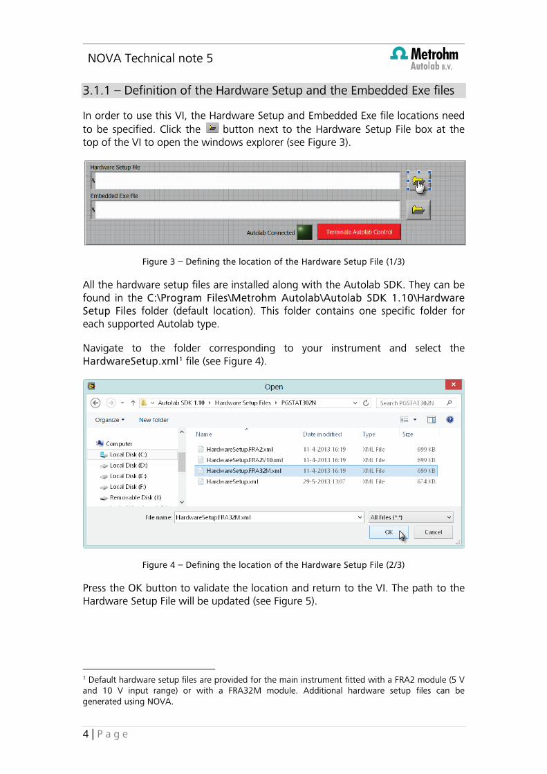
In order to use this VI, the Hardware Setup and Embedded Exe file locations need to be specified. Click the button next to the Hardware Setup File box at the top of the VI to open the windows explorer (see Figure 3).
Figure 3 – Defining the location of the Hardware Setup File (1/3)
All the hardware setup files are installed along with the Autolab SDK. They can be found in the C:\Program Files\Metrohm Autolab\Autolab SDK 1.10\Hardware Setup Files folder (default location). This folder contains one specific folder for each supported Autolab type.
Navigate to the folder corresponding to your instrument and select the HardwareSetup.xml1 file (see Figure 4).
Figure 4 – Defining the location of the Hardware Setup File (2/3)
Press the OK button to validate the location and return to the VI. The path to the Hardware Setup File will be updated (see Figure 5).
1 Default hardware setup files are provided for the main instrument fitted with a FRA2 module (5 V and 10 V input range) or with a FRA32M module. Additional hardware setup files can be generated using NOVA.
NOVA Technical Note 5
5 | P a g e
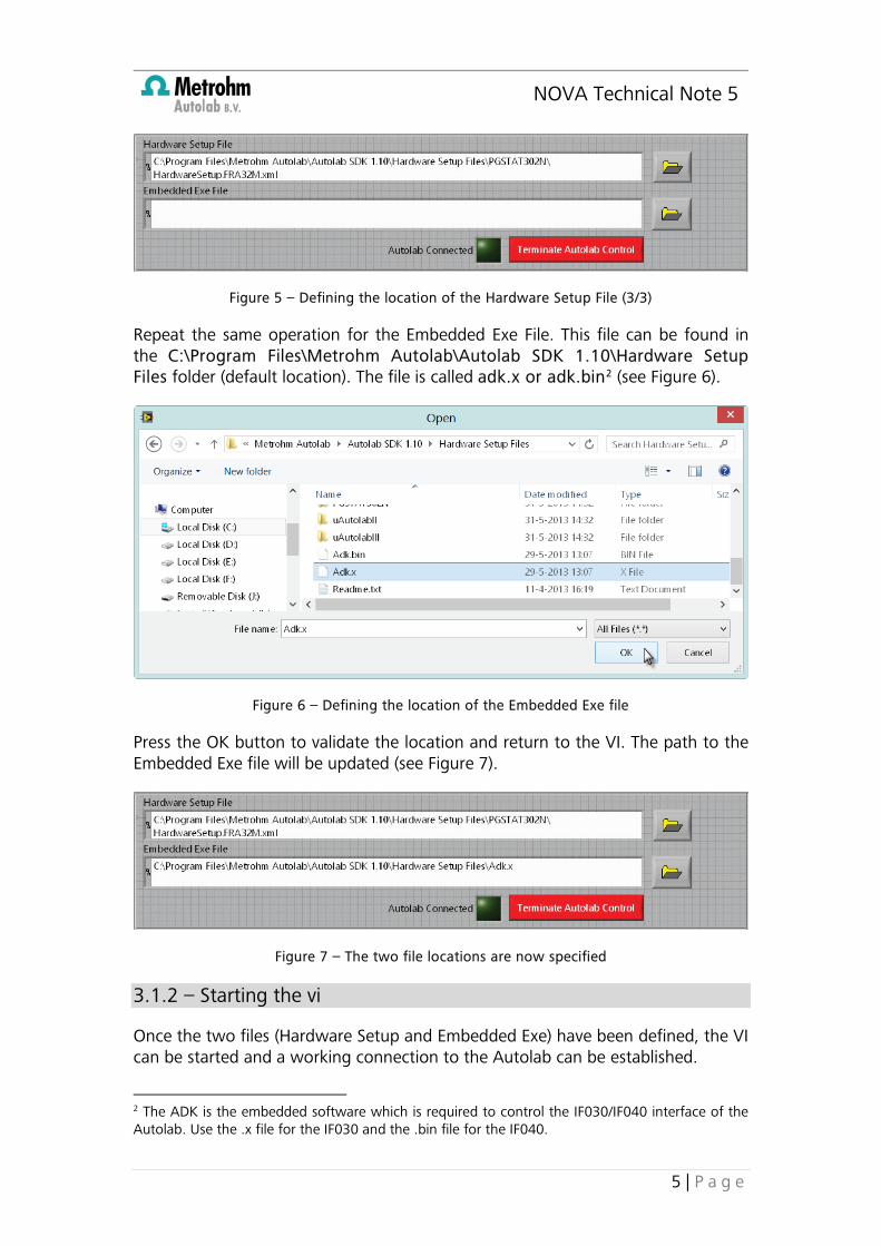
Figure 5 – Defining the location of the Hardware Setup File (3/3)
Repeat the same operation for the Embedded Exe File. This file can be found in the C:\Program Files\Metrohm Autolab\Autolab SDK 1.10\Hardware Setup Files folder (default location). The file is called adk.x or adk.bin2 (see Figure 6).
Figure 6 – Defining the location of the Embedded Exe file
Press the OK button to validate the location and return to the VI. The path to the Embedded Exe file will be updated (see Figure 7).
Figure 7 – The two file locations are now specified
3.1.2 – Starting the vi
Once the two files (Hardware Setup and Embedded Exe) have been defined, the VI can be started and a working connection to the Autolab can be established.
2 The ADK is the embedded software which is required to control the IF030/IF040 interface of the Autolab. Use the .x file for the IF030 and the .bin file for the IF040.

NOVA Technical note 5
6 | P a g e
Press the button located in the toolbar of LabVIEW (see Figure 8).
Figure 8 – Pressing the button starts the VI
The VI will start and the Embedded Exe file will be uploaded to the Autolab. This can take a few seconds. Once the connection has been established, the Autolab Connected indicator will switch to green (see Figure 9).
Figure 9 – The Autolab Connected indicator will be switched on when the connection has been established
Note
It is possible to release the connection to the Autolab at any time by pressing the red Terminate Autolab Control button.
Note
If no FRA2 calibration has been defined, the following warning will be displayed before the Autolab is connected (see Figure 10). Refer to the Getting started of NOVA for more information on how to import the FRA2 calibration file. Click OK to continue without the file.

NOVA Technical Note 5
7 | P a g e
Figure 10 – If the FRA2 calibration file is not found, the following message will be displayed
3.1.3 – Loading a .nox procedure
The Autolab SDK can run a pre-existing NOVA procedure by reading the .nox file. The Autolab SDK comes with a number of example procedures. Using the same mechanism as for the Hardware Setup and the Embedded Exe files, click the button next to the Load procedure box and navigate to the folder containing the procedure files (default: C:\Program Files\Metrohm Autolab\Autolab SDK 1.10\Standard Nova Procedures). Select the Cyclic voltammetry.nox procedure file. Click OK to validate the location of the file and return to the VI (see Figure 11).
Figure 11 – Defining the location of the NOVA .nox procedure file
Once the path to the procedure file has been defined, press the large blue Load button, , located on the right-hand side of the button (see Figure 12). This will load the contents of the .nox file.
Figure 12 – Loading the procedure file
Note
The location of the procedure file can be written in the Load Procedure box directly.

NOVA Technical note 5
8 | P a g e
3.1.4 – Changing a procedure parameter
The .nox files are used ‘as provided’. This means that it is not possible to change the procedure itself (this must be done in NOVA). It is however possible to change one or more command parameters in the loaded procedure.
Press the Load procedure parameters button, , in order to load all the procedure parameters in the VI (see Figure 13).
Figure 13 – Press the Load procedure parameters button to load all the parameters of the procedure
Click the drop-down list on the left hand side of the VI to choose the command in the procedure that needs to be edited. In this example, we will change the Upper vertex potential value. Select the CV staircase command from the Command name drop-down list (see Figure 14).
Figure 14 – Selecting the command from the list
Repeat the same for the Command parameter drop-down list and select the Upper vertex potential from the list (see Figure 15).

NOVA Technical Note 5
9 | P a g e
Figure 15 – Selecting the Upper vertex potential from the command parameter list
The current parameter value will be displayed in the box on the right-hand side of the VI. Since the value of the Upper vertex potential is 1 V in the .nox file, the value displayed should be 1.
Type the value of 1.2 in the Edit parameter field and press the Update value button, (see Figure 16).
Figure 16 – Press the Update value button to change the value of the Command parameter
The VI will be updated and the new value will be displayed in the Current parameter field.
NOVA Technical note 5
10 | P a g e
3.1.5 – Setting up the display settings
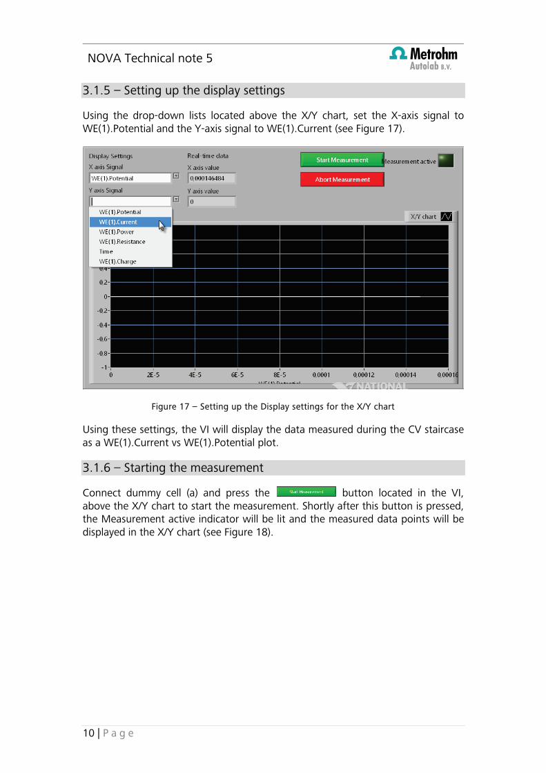
Using the drop-down lists located above the X/Y chart, set the X-axis signal to WE(1).Potential and the Y-axis signal to WE(1).Current (see Figure 17).
Figure 17 – Setting up the Display settings for the X/Y chart
Using these settings, the VI will display the data measured during the CV staircase as a WE(1).Current vs WE(1).Potential plot.
3.1.6 – Starting the measurement
Connect dummy cell (a) and press the button located in the VI, above the X/Y chart to start the measurement. Shortly after this button is pressed, the Measurement active indicator will be lit and the measured data points will be displayed in the X/Y chart (see Figure 18).

NOVA Technical Note 5
11 | P a g e
Figure 18 – Performing the measurement on dummy cell (a)
When the measurement is complete, the Measurement active indicator will switch off. It is possible to abort the measurement at any time by pressing the Abort Measurement button, .
3.1.7 – Loading the data after the measurement
The data displayed in the X/Y chart during the measurement is not quite ‘real-time’. This is a limitation of the LabVIEW software. In reality, the measurement is always carefully timed by the Autolab, through the embedded controller. At high sampling rate, the data displayed in the X/Y chart could be distorted.
After the measurement is finished, it is possible to inspect the measured data points more carefully. Click the button located at the bottom of the VI to load the data points from the last measurement (see Figure 19).

NOVA Technical note 5
12 | P a g e
Figure 19 – Loading the data from the last measurement
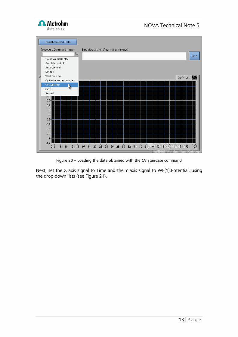
Once the data has been loaded, it is possible to display the data points obtained with each measurement or data handling command in the .nox procedure.
Using the drop-down list, select the CV staircase command to load the data obtained with this command (see Figure 20).
NOVA Technical Note 5
13 | P a g e
Figure 20 – Loading the data obtained with the CV staircase command
Next, set the X axis signal to Time and the Y axis signal to WE(1).Potential, using the drop-down lists (see Figure 21).

NOVA Technical note 5
14 | P a g e
Figure 21 – Setting the X and Y axis signals
All the data points measured during CV staircase command will be displayed accurately in the second X/Y chart (see Figure 22).
Figure 22 – The WE(1).Potential vs Time plot
NOVA Technical Note 5
15 | P a g e
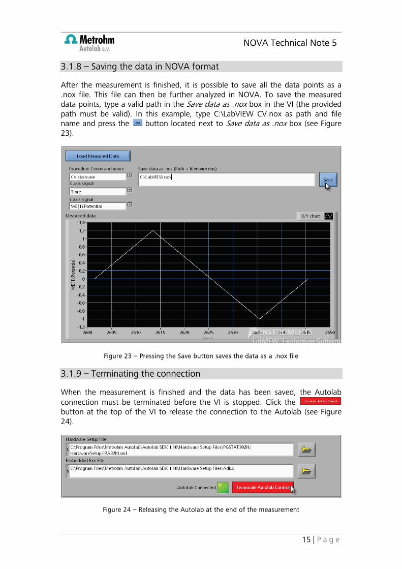
3.1.8 – Saving the data in NOVA format
After the measurement is finished, it is possible to save all the data points as a .nox file. This file can then be further analyzed in NOVA. To save the measured data points, type a valid path in the Save data as .nox box in the VI (the provided path must be valid). In this example, type C:\LabVIEW CV.nox as path and file name and press the button located next to Save data as .nox box (see Figure 23).
Figure 23 – Pressing the Save button saves the data as a .nox file
3.1.9 – Terminating the connection
When the measurement is finished and the data has been saved, the Autolab connection must be terminated before the VI is stopped. Click the button at the top of the VI to release the connection to the Autolab (see Figure 24).
Figure 24 – Releasing the Autolab at the end of the measurement

NOVA Technical note 5
16 | P a g e
Once the Autolab control has been terminated, the VI will stop completely.
3.2 – TN#5 FRA example (A).vi
Double click the [TN#5] FRA example (A).vi in the Advanced Examples group to load it. This VI works in the same way as the previous one. First the location of the Hardware Setup and the Embedded Exe files must be provided. Then the VI can be started and a connection with the Autolab is created. A .nox procedure for a FRA measurement can then be provided and loaded (see Figure 25). An example of a FRA measurement procedure is provided in the C:\Program Files\Metrohm Autolab\Autolab SDK 1.10\Standard Nova Procedures folder.
Figure 25 – Using the FRA example VI
Once the procedure has been loaded (do not forget to press the button), the procedure can be started. Pressing the button will start the FRA frequency scan in potentiostatic mode.
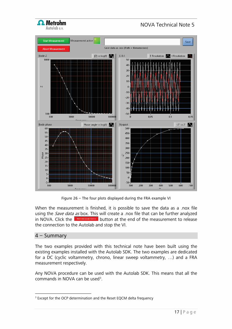
During the measurement, four plots will be shown (see Figure 26):
• Bode plot, Z • Resolution plot for Current and Potential • Bode plot, phase • Nyquist plot
Warning
Always remember to terminate the Autolab control before stopping the VI. If the VI is stopped before the Autolab control is released, LabVIEW will crash. This is a problem of LabVIEW.
NOVA Technical Note 5
17 | P a g e
Figure 26 – The four plots displayed during the FRA example VI
When the measurement is finished, it is possible to save the data as a .nox file using the Save data as box. This will create a .nox file that can be further analyzed in NOVA. Click the button at the end of the measurement to release the connection to the Autolab and stop the VI.
4 – Summary
The two examples provided with this technical note have been built using the existing examples installed with the Autolab SDK. The two examples are dedicated for a DC (cyclic voltammetry, chrono, linear sweep voltammetry, …) and a FRA measurement respectively.
Any NOVA procedure can be used with the Autolab SDK. This means that all the commands in NOVA can be used3.
3 Except for the OCP determination and the Reset EQCM delta frequency