1

HOW TO GO ABOUT DATA GENERATION AND ANALYSIS (Lecture 11, 2009_03_08) ### Please recall my remarks in Lecture 1 about the nature of the lecture notes. ### Outlines of „lit reviews” ? Steve Levitt’s (J.B.Clark medal 2003) Rules of thumb for successful empirical research 1) A paper must ask a good question - one that has never been asked - you do not know the answer in advance - no matter what answer you get it will be interesting - others were getting a wrong answer so far 2) A paper should have an “idea” - a clever new way of answering an old question - a new source of identification - uncovering a relationship nobody has thought of so far - a new econometric method 3) The simpler the execution the better - present data and results in as raw a form as possible - build-in complexity later - avoid too many assumptions when constructing more complicated estimators - people should see where your results are coming from 4) Be certain you have the right answer - check robustness to death - think through all the implications of your model for the results 5) Interpret your results - throwing regression coefficients into a table is not enough - what’s the economic significance of your results? - do some cost-benefit analysis, implications for policy, etc.. 6) Become an expert - learn as much as you can about the institutional background - some first-hand, insider experience will tell you far more than the books 7) When you should, fail quickly and leave the sunk costs - if there’s nothing in the data, dump it - if the data goes the wrong way at the first glimpse, drop the project 8) Practice makes perfect

2

### Review ON SUBJECT POOLS AND LEVELS OF REASONING (Lecture 10, 2009_03_08) ### Bosch-Domenech et al., One. Two. (three), infinity, … : newspaper and lab beauty-contest experiments (AER 2002) BCG (e.g., Nagel AER 1995): Players submit a number between 0 and 100. The winner is the person whose number is closest to p times the average of all submitted numbers, where 0 < p < 1, and here 2/3. Winners split prize. Design and Implementation

- Historically, lots of lab experiments … (Nagel 1995 and many others including new ones reported in this paper)

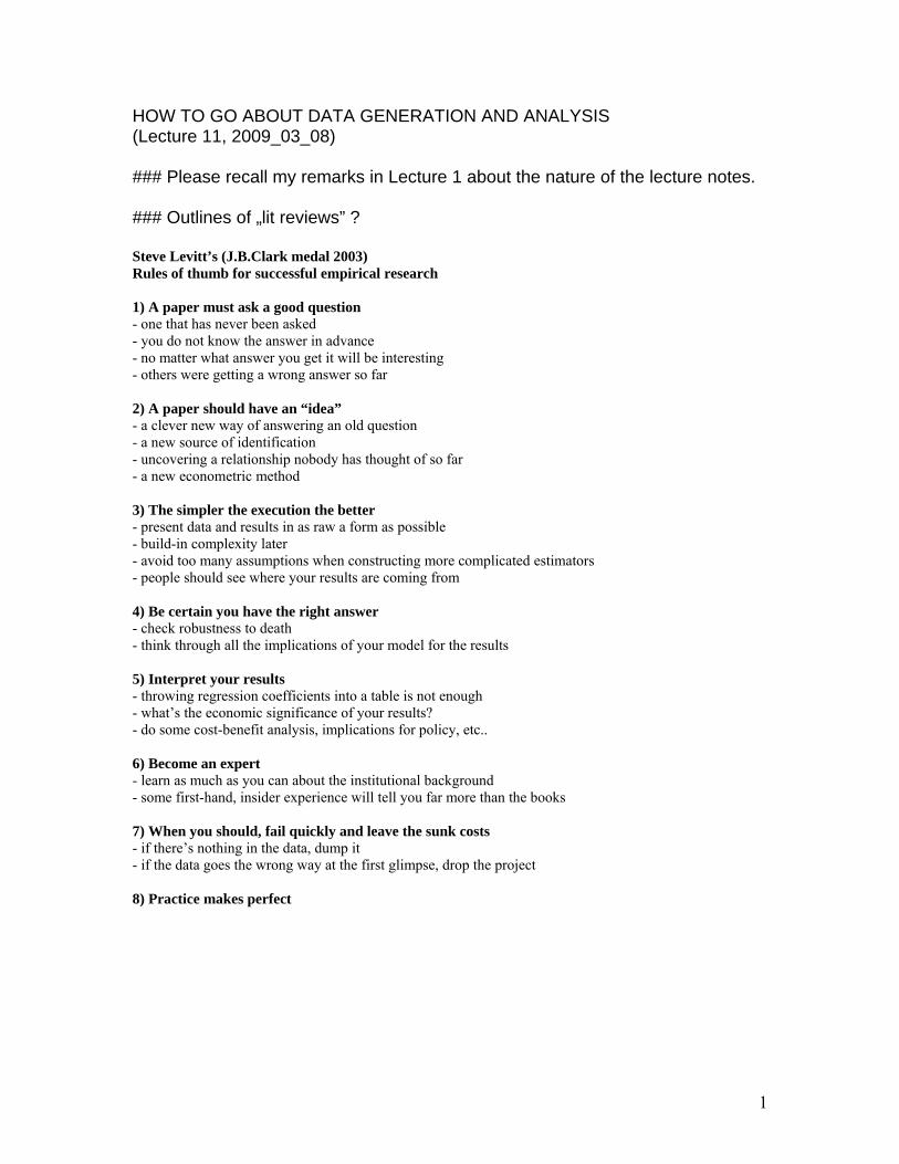
- Here also reported newspaper (artefactual) experiments with readers of Financial Times, Spektrum der Wissenschaft, and Expansion

- (p.p. 1693 – 7)

(a) subjects’ socio-demographic characteristics (b) information acquisition (c) coalition formation

3

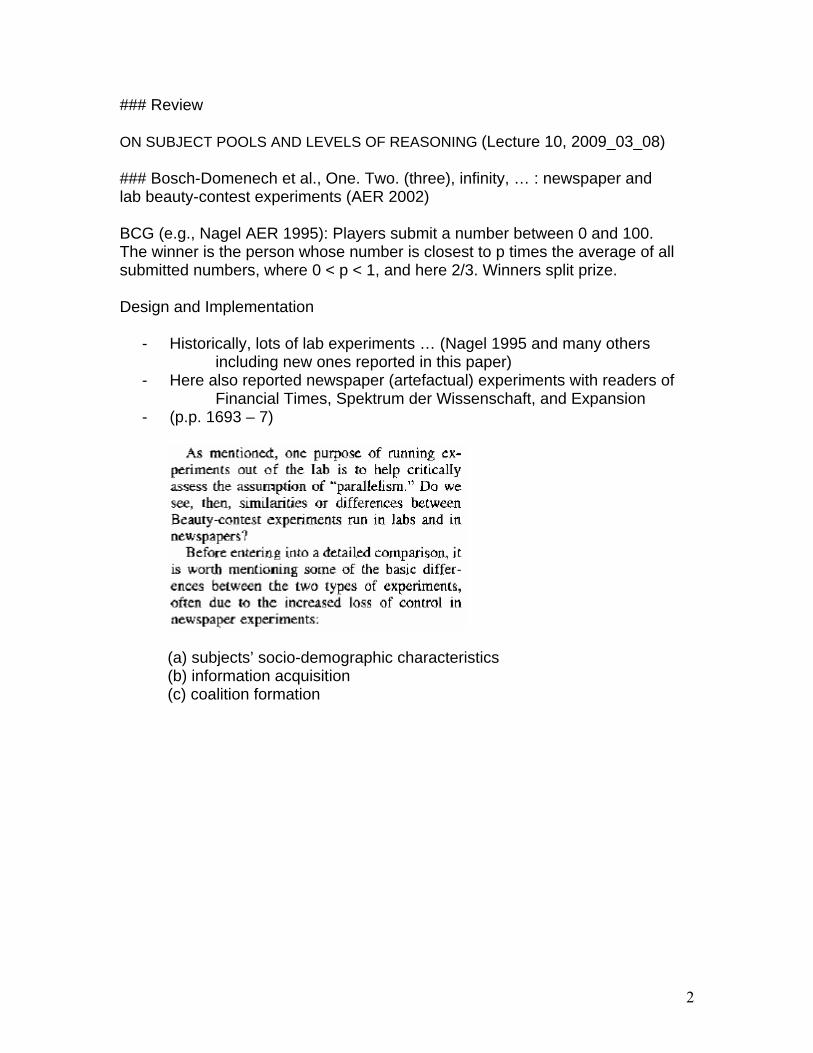
Results (see also the various facts extracted in the lecture notes from the article):

Summary

- Yes, subject pools do matter but … (qualitatively the same picture) - People of various walks of life do not engage in many steps of reasoning - “Experimenters” do rather well (in the sense that they figure out what

others think), at least in this experiment

4

### Johnson et al., Detecting failures of backward induction: Monitoring information search in sequential bargaining (JET 2002)

Motivation

To tease apart why people do not manage to implement the subgame-perfect solution in alternating offer games [explain specifically how used in the present paper], or in simple bargaining games for that matter: - Is it due to social preferences? - Is it due to cognitive limitations?

Design and implementation Use MouseLab and undergraduate students to find an answer. Three experimental studies:

- Bargaining with other players - Bargaining with robots and instructions - turning off “social preferences’ - also, teaching subjects - Mixing trained and untrained subjects

Each subject plays 8 (16, 16) three-round alternating offer games, rematched each round in group of 10 with another member of the group. Payment in cash at the end according to performance (half of dollar earnings and show-up fee)

5

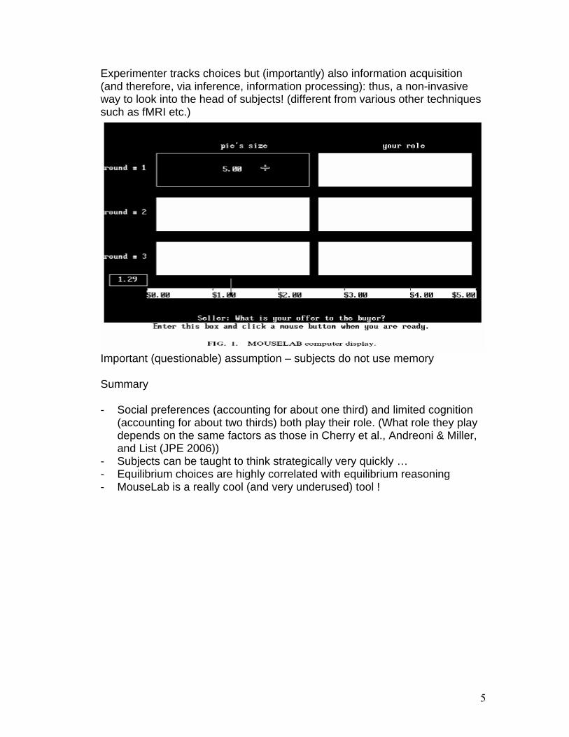
Experimenter tracks choices but (importantly) also information acquisition (and therefore, via inference, information processing): thus, a non-invasive way to look into the head of subjects! (different from various other techniques such as fMRI etc.)

Important (questionable) assumption – subjects do not use memory Summary - Social preferences (accounting for about one third) and limited cognition

(accounting for about two thirds) both play their role. (What role they play depends on the same factors as those in Cherry et al., Andreoni & Miller, and List (JPE 2006))

- Subjects can be taught to think strategically very quickly … - Equilibrium choices are highly correlated with equilibrium reasoning - MouseLab is a really cool (and very underused) tool !

6

### Rubinstein, Instinctive and Cognitive Reasoning: A study of response times (EJ 2007) Motivation Rather than fMRI [to be discussed later in this course] or similar expensive, small-sample (and hence noisy) studies, Rubinstein wants “to explore the deliberation process of decision makers based on their response times.” (p. 1244) Definition “Response time [RT] is defined here as the number of seconds between the moment that our server receives the request for a problem until the moment that an answer is returned to the server.” (p. 1245, see also p. 1257, 5.(a) )

- no control for differential server speed, or transfer speeds - no control for differential speed of reading etc.

“The magic of a large sample gives us a clear picture of the relative time responses.” (p. 22; indeed statistical tests highly significant – no surprise given the numbers involved.; see p. 1257, 5.(b))

(p. 1257) -> worksheet [recall earlier lecture on financial and social incentives]

7

Basic working hypothesis Action that require lesser response time are more instinctive (i.e., on the basis of an emotional response); those requiring more response time are more cognitive. [We’ll return to this issue also in L 13, 14 when we discuss issues in neuroeconomics.] Basic methodology Classify “intuitively” (“I have done so intuitively.” p. 1245, see also p. 1258, 5.(c)):

See related questions on worksheet.

8

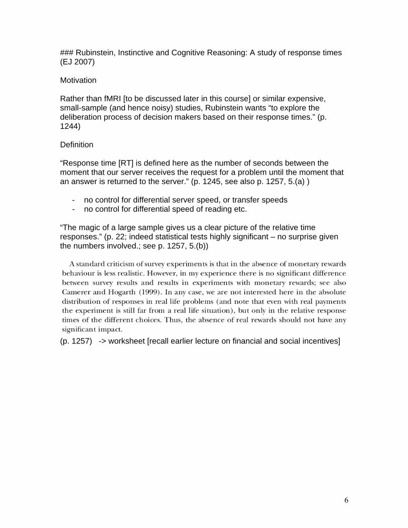
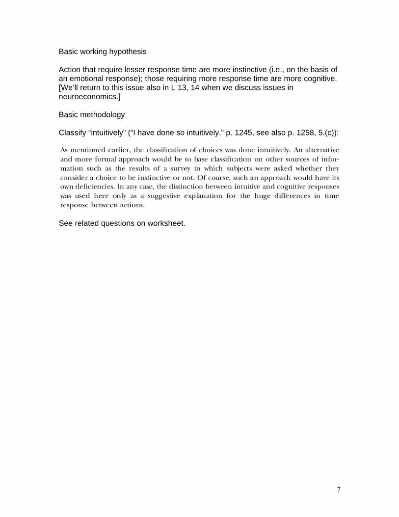
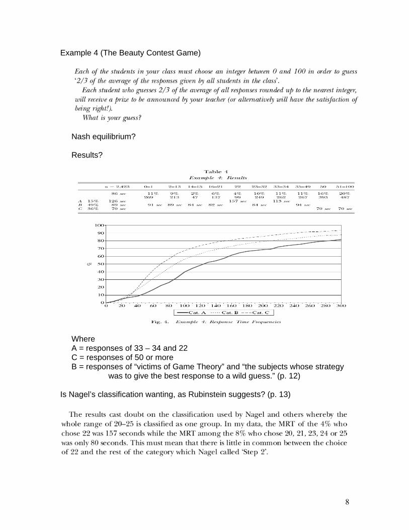
Example 4 (The Beauty Contest Game)

Nash equilibrium? Results?

Where A = responses of 33 – 34 and 22 C = responses of 50 or more B = responses of “victims of Game Theory” and “the subjects whose strategy

was to give the best response to a wild guess.” (p. 12)

Is Nagel’s classification wanting, as Rubinstein suggests? (p. 13)

9

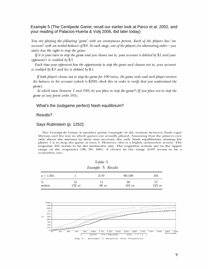
Example 5 (The Centipede Game; recall our earlier look at Parco et al. 2002, and your reading of Palacios-Huerta & Volij 2006, tbd later today)

What’s the (subgame perfect) Nash equilibrium? Results? Says Rubinstein (p. 1252):

10

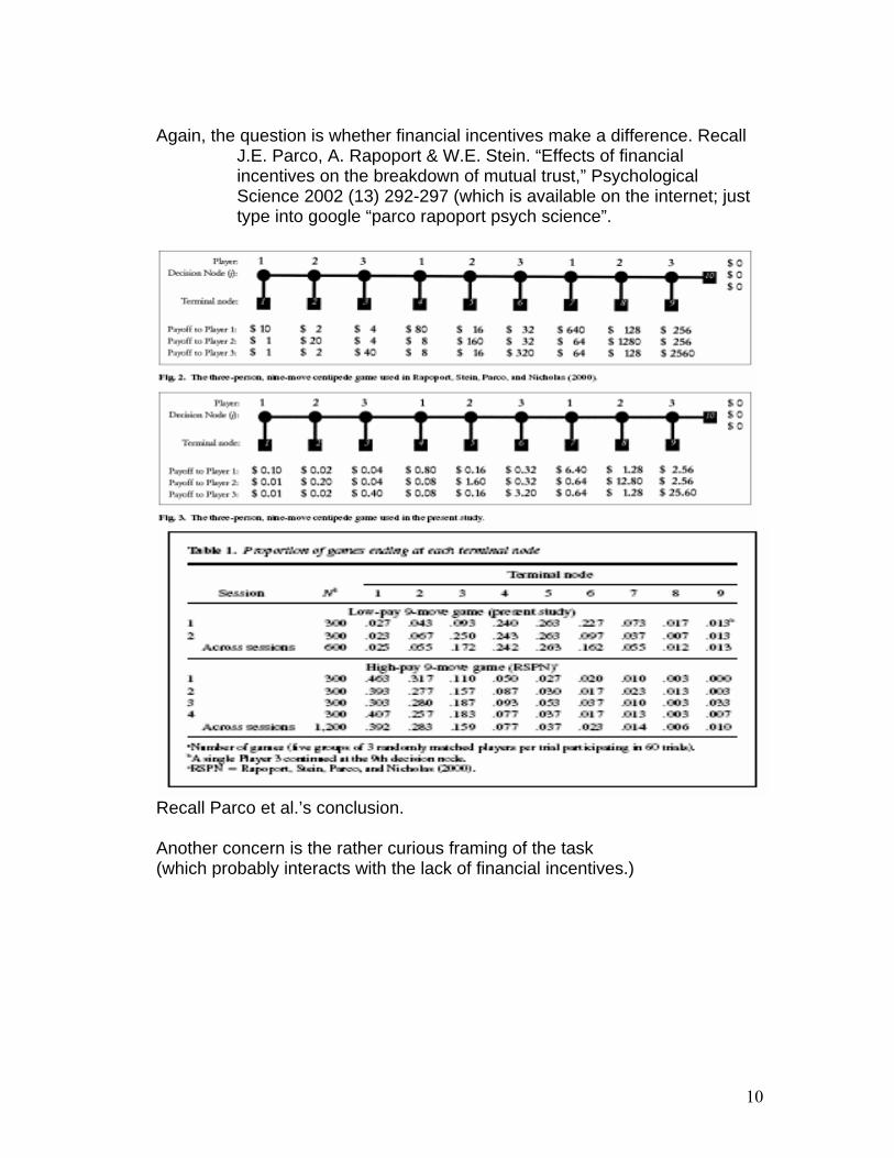
Again, the question is whether financial incentives make a difference. Recall

J.E. Parco, A. Rapoport & W.E. Stein. “Effects of financial incentives on the breakdown of mutual trust,” Psychological Science 2002 (13) 292-297 (which is available on the internet; just type into google “parco rapoport psych science”.

Recall Parco et al.’s conclusion. Another concern is the rather curious framing of the task (which probably interacts with the lack of financial incentives.)

11

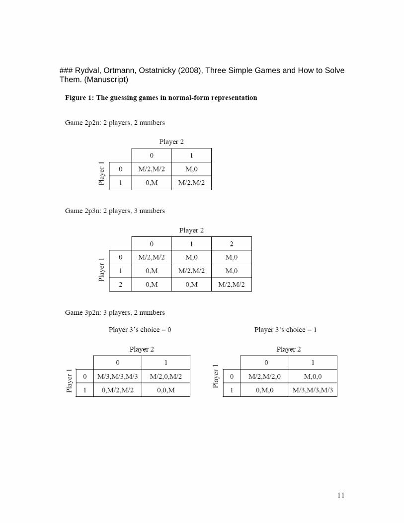
### Rydval, Ortmann, Ostatnicky (2008), Three Simple Games and How to Solve Them. (Manuscript)

12

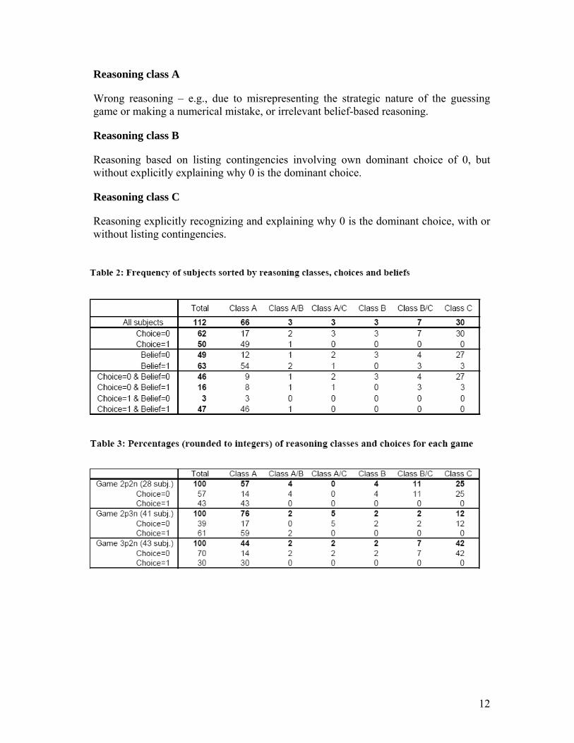
Reasoning class A

Wrong reasoning – e.g., due to misrepresenting the strategic nature of the guessing game or making a numerical mistake, or irrelevant belief-based reasoning.

Reasoning class B

Reasoning based on listing contingencies involving own dominant choice of 0, but without explicitly explaining why 0 is the dominant choice.

Reasoning class C

Reasoning explicitly recognizing and explaining why 0 is the dominant choice, with or without listing contingencies.

13

### Kovalchik, Camerer, Grether, Plott, Allman, Aging and decision making: a comparison between neurologically healthy elderly and young individuals (JEBO 2005) How many experiments on how many populations? Specifically what are the populations? 4, 2, neurologically healthy elderly (ave age 82, N = 50, 70 % female) and young individuals (probably from PCC, N = 51, 51 % female ) What are the tasks used in those experiments?

- Confidence (exploring meta-knowledge, see Hertwig & Ortmann book chapter, lecture 9)

- decisions under uncertainty - differences between WTP – WTA (as in Plott Zeiler) - strategic thinking (as in Bosch-Domenech et al)

What exactly was the confidence task? (Make sure you read Appendix A; do you see any problem with the questions?)

- 20 trivia questions (general knowledge questions? These questions seem to reflect the age of the experimenters! They may be trivia questions but I doubt whether they are legitimate general knowledge questions!)

- all questions two possible answers - subjects had to try to give answer and provide a confidence assessment of their answer

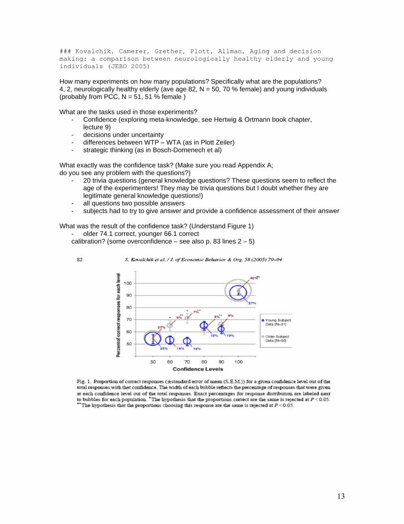
What was the result of the confidence task? (Understand Figure 1)

- older 74.1 correct, younger 66.1 correct calibration? (some overconfidence – see also p. 83 lines 2 – 5)

14

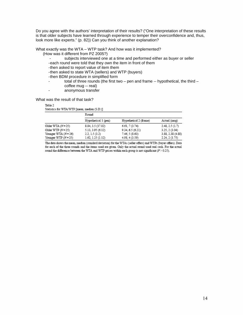
Do you agree with the authors’ interpretation of their results? (“One interpretation of these results is that older subjects have learned through experience to temper their overconfidence and, thus, look more like experts.” (p. 82)) Can you think of another explanation? What exactly was the WTA – WTP task? And how was it implemented?

(How was it different from PZ 2005?) - subjects interviewed one at a time and performed either as buyer or seller

- each round were told that they own the item in front of them - then asked to report value of item them - then asked to state WTA (sellers) and WTP (buyers) - then BDM procedure in simplified form - total of three rounds (the first two – pen and frame -- hypothetical, the third –

coffee mug -- real) - anonymous transfer

What was the result of that task?

15

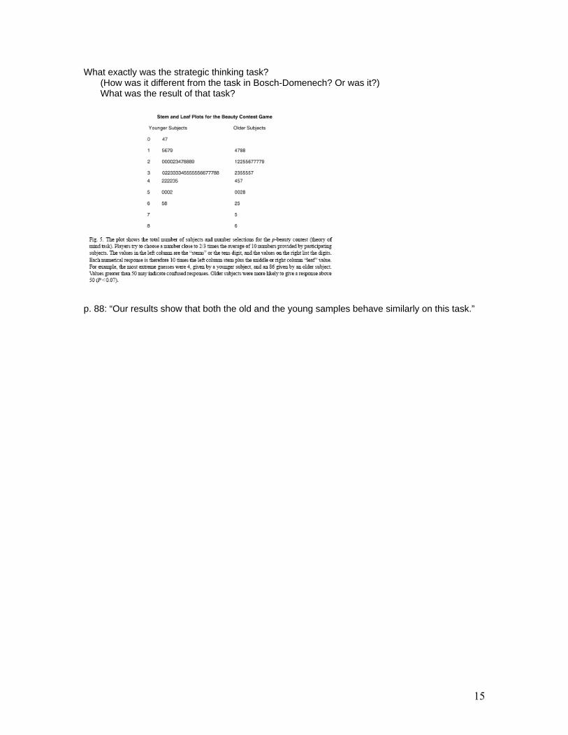
What exactly was the strategic thinking task? (How was it different from the task in Bosch-Domenech? Or was it?) What was the result of that task?

p. 88: “Our results show that both the old and the young samples behave similarly on this task.”

16

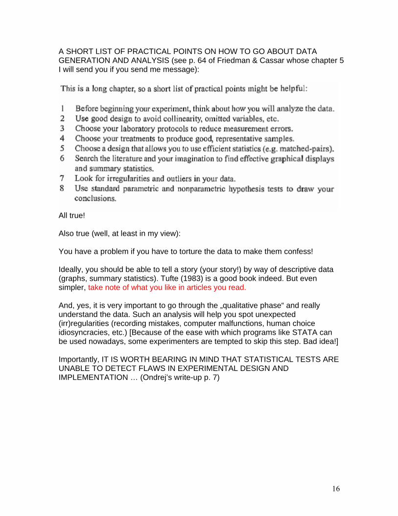
A SHORT LIST OF PRACTICAL POINTS ON HOW TO GO ABOUT DATA GENERATION AND ANALYSIS (see p. 64 of Friedman & Cassar whose chapter 5 I will send you if you send me message):

All true! Also true (well, at least in my view): You have a problem if you have to torture the data to make them confess! Ideally, you should be able to tell a story (your story!) by way of descriptive data (graphs, summary statistics). Tufte (1983) is a good book indeed. But even simpler, take note of what you like in articles you read. And, yes, it is very important to go through the „qualitative phase“ and really understand the data. Such an analysis will help you spot unexpected (irr)regularities (recording mistakes, computer malfunctions, human choice idiosyncracies, etc.) [Because of the ease with which programs like STATA can be used nowadays, some experimenters are tempted to skip this step. Bad idea!] Importantly, IT IS WORTH BEARING IN MIND THAT STATISTICAL TESTS ARE UNABLE TO DETECT FLAWS IN EXPERIMENTAL DESIGN AND IMPLEMENTATION … (Ondrej’s write-up p. 7)

17

A little excursion of a more general nature: The following text has been copied and edited from a wonderful homepage that I recommend to you enthusiastically: http://www.socialresearchmethods.net/

It’s an excellent resource for social science reseach methods.

Four interrelated components that influence the conclusions you might reach from a statistical test in a research project [Sadly, it has to be said that most experimentalists do not think much about the interrelatedness of these components, or any of these components other than the alpha level; but the prevalence of a bad practice does not mean, that one ought, or has to, adopt it]:

The four components are:

sample size, or the number of units (e.g., people) accessible to the study effect size, or the salience of the treatment relative to the noise in measurement alpha level (α, or significance level), or the odds that the observed result is due to chance power, or the odds that you will observe a treatment effect when it occurs

Given values for any three of these components, it is possible to compute the value of the fourth. For instance, you might want to determine what a reasonable sample size would be for a study. If you could make reasonable estimates of the effect size, alpha level and power, it would be simple to compute (or, more likely, look up in a table) the sample size.

Some of these components will be more manipulable than others depending on the circumstances of the project. For example, if the project is an evaluation of an educational program, the sample size is predetermined. Or, if the drug dosage in a program has to be small due to its potential negative side effects, the effect size may consequently be small. The goal is to achieve a balance of the four components that allows the maximum level of power to detect an effect if one exists, given programmatic, logistical or financial constraints on the other components. Of course, financial constraints are always a concern to experimental economists.

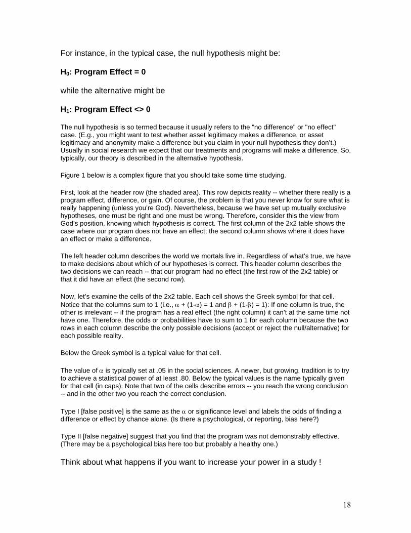
Figure 1 shows the basic decision matrix involved in a statistical conclusion. All statistical conclusions involve constructing two mutually exclusive hypotheses, termed the null (labeled H0) and alternative (labeled H1) hypothesis. Together, the hypotheses describe all possible outcomes with respect to the inference. The central decision involves determining which hypothesis to accept and which to reject.

18

For instance, in the typical case, the null hypothesis might be:

H0: Program Effect = 0

while the alternative might be

H1: Program Effect <> 0

The null hypothesis is so termed because it usually refers to the "no difference" or "no effect" case. (E.g., you might want to test whether asset legitimacy makes a difference, or asset legitimacy and anonymity make a difference but you claim in your null hypothesis they don’t.) Usually in social research we expect that our treatments and programs will make a difference. So, typically, our theory is described in the alternative hypothesis.

Figure 1 below is a complex figure that you should take some time studying.

First, look at the header row (the shaded area). This row depicts reality -- whether there really is a program effect, difference, or gain. Of course, the problem is that you never know for sure what is really happening (unless you’re God). Nevertheless, because we have set up mutually exclusive hypotheses, one must be right and one must be wrong. Therefore, consider this the view from God’s position, knowing which hypothesis is correct. The first column of the 2x2 table shows the case where our program does not have an effect; the second column shows where it does have an effect or make a difference.

The left header column describes the world we mortals live in. Regardless of what’s true, we have to make decisions about which of our hypotheses is correct. This header column describes the two decisions we can reach -- that our program had no effect (the first row of the 2x2 table) or that it did have an effect (the second row).

Now, let’s examine the cells of the 2x2 table. Each cell shows the Greek symbol for that cell. Notice that the columns sum to 1 (i.e., α + (1-α) = 1 and β + (1-β) = 1): If one column is true, the other is irrelevant -- if the program has a real effect (the right column) it can’t at the same time not have one. Therefore, the odds or probabilities have to sum to 1 for each column because the two rows in each column describe the only possible decisions (accept or reject the null/alternative) for each possible reality.

Below the Greek symbol is a typical value for that cell.

The value of α is typically set at .05 in the social sciences. A newer, but growing, tradition is to try to achieve a statistical power of at least .80. Below the typical values is the name typically given for that cell (in caps). Note that two of the cells describe errors -- you reach the wrong conclusion -- and in the other two you reach the correct conclusion.

Type I [false positive] is the same as the α or significance level and labels the odds of finding a difference or effect by chance alone. (Is there a psychological, or reporting, bias here?)

Type II [false negative] suggest that you find that the program was not demonstrably effective. (There may be a psychological bias here too but probably a healthy one.)

Think about what happens if you want to increase your power in a study !

19

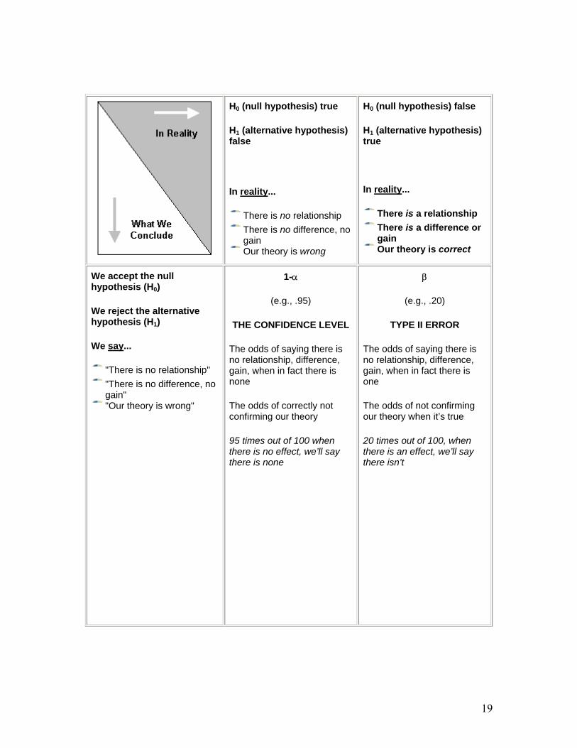
H0 (null hypothesis) true

H1 (alternative hypothesis) false

In reality...

There is no relationship There is no difference, no gain Our theory is wrong

H0 (null hypothesis) false

H1 (alternative hypothesis) true

In reality...

There is a relationship There is a difference or gain Our theory is correct

We accept the null hypothesis (H0)

We reject the alternative hypothesis (H1)

We say...

"There is no relationship"

"There is no difference, no gain" "Our theory is wrong"

1-α

(e.g., .95)

THE CONFIDENCE LEVEL

The odds of saying there is no relationship, difference, gain, when in fact there is none

The odds of correctly not confirming our theory

95 times out of 100 when there is no effect, we’ll say there is none

β

(e.g., .20)

TYPE II ERROR

The odds of saying there is no relationship, difference, gain, when in fact there is one

The odds of not confirming our theory when it’s true

20 times out of 100, when there is an effect, we’ll say there isn’t

20

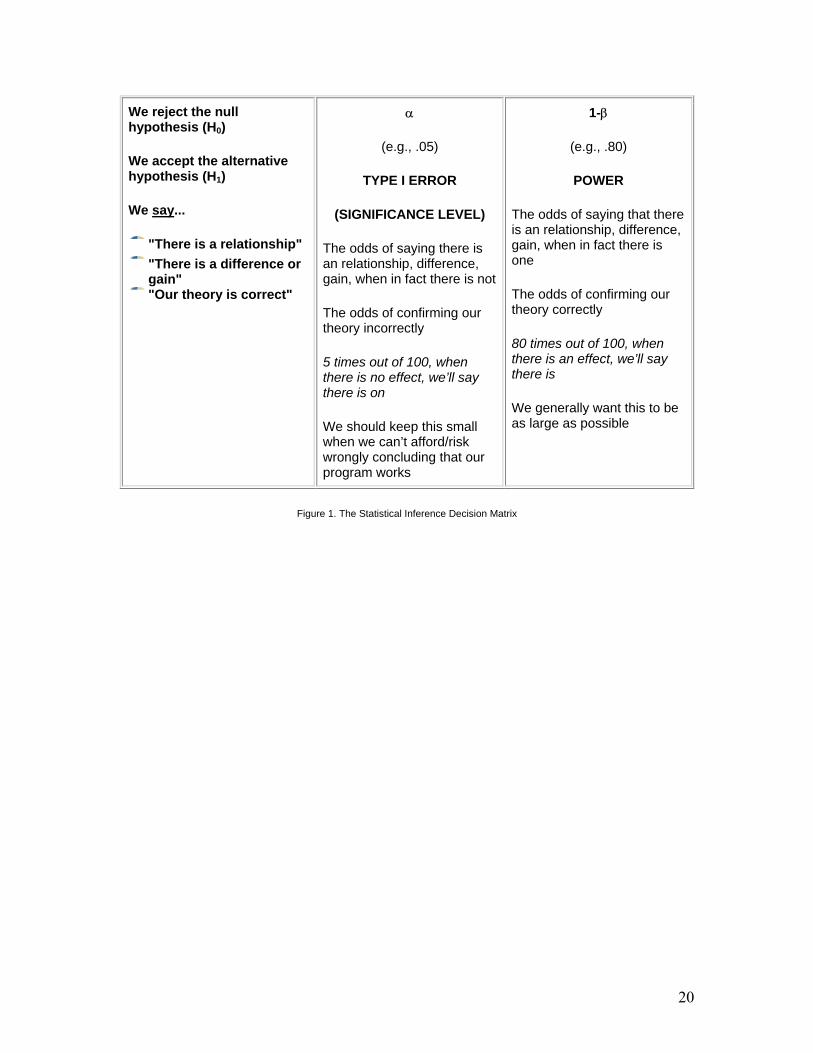
We reject the null hypothesis (H0)

We accept the alternative hypothesis (H1)

We say...

"There is a relationship"

"There is a difference or gain" "Our theory is correct"

α

(e.g., .05)

TYPE I ERROR

(SIGNIFICANCE LEVEL)

The odds of saying there is an relationship, difference, gain, when in fact there is not

The odds of confirming our theory incorrectly

5 times out of 100, when there is no effect, we’ll say there is on

We should keep this small when we can’t afford/risk wrongly concluding that our program works

1-β

(e.g., .80)

POWER

The odds of saying that there is an relationship, difference, gain, when in fact there is one

The odds of confirming our theory correctly

80 times out of 100, when there is an effect, we’ll say there is

We generally want this to be as large as possible

Figure 1. The Statistical Inference Decision Matrix

21

We often talk about alpha (α) and beta (β) using the language of "higher" and "lower." For instance, we might talk about the advantages of a higher or lower α-level in a study. You have to be careful about interpreting the meaning of these terms. When we talk about higher α-levels, we mean that we are increasing the chance of a Type I Error. Therefore, a lower α-level actually means that you are conducting a more rigorous test. With all of this in mind, let’s consider a few common associations evident in the table. You should convince yourself of the following:

the lower the α, the lower the power; the higher the α, the higher the power the lower the α, the less likely it is that you will make a Type I Error (i.e., reject the null when it’s true) the lower the α, the more "rigorous" the test an α of .01 (compared with .05 or .10) means the researcher is being relatively careful, s/he is only willing to risk being wrong 1 in a 100 times in rejecting the null when it’s true (i.e., saying there’s an effect when there really isn’t) an α of .01 (compared with .05 or .10) limits one’s chances of ending up in the bottom row, of concluding that the program has an effect. This means that both your statistical power and the chances of making a Type I Error are lower. an α of .01 means you have a 99% chance of saying there is no difference when there in fact is no difference (being in the upper left box) increasing α (e.g., from .01 to .05 or .10) increases the chances of making a Type I Error (i.e., saying there is a difference when there is not), decreases the chances of making a Type II Error (i.e., saying there is no difference when there is) and decreases the rigor of the test increasing α (e.g., from .01 to .05 or .10) increases power because one will be rejecting the null more often (i.e., accepting the alternative) and, consequently, when the alternative is true, there is a greater chance of accepting it (i.e., power)

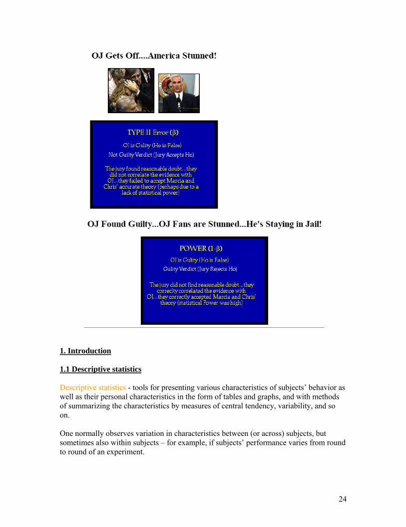
Robert M. Becker at Cornell University illustrates these concepts masterfully, and entertainingly, by way of the OJ Simpson trial (note that this is actually a very nice illustration of the advantages of contextualization although there may be order effects here ): http://www.socialresearchmethods.net/OJtrial/ojhome.htm H0: OJ Simpson was innocent

(although our theory is that in fact he was guilty as charged) HA: Guilty as charged (double murder) Can H0 be rejected, at a high level of confidence? I.e. …

22

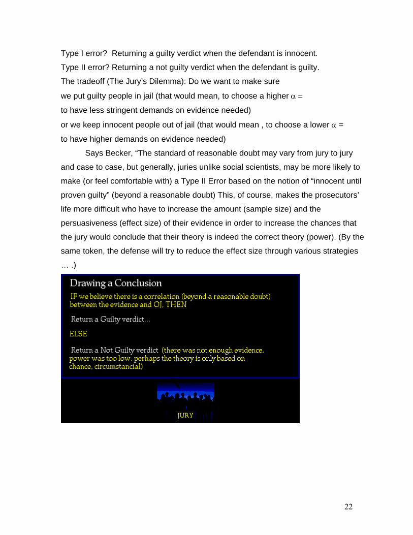
Type I error? Returning a guilty verdict when the defendant is innocent.

Type II error? Returning a not guilty verdict when the defendant is guilty.

The tradeoff (The Jury’s Dilemma): Do we want to make sure

we put guilty people in jail (that would mean, to choose a higher α =

to have less stringent demands on evidence needed)

or we keep innocent people out of jail (that would mean , to choose a lower α =

to have higher demands on evidence needed)

Says Becker, “The standard of reasonable doubt may vary from jury to jury

and case to case, but generally, juries unlike social scientists, may be more likely to

make (or feel comfortable with) a Type II Error based on the notion of “innocent until

proven guilty” (beyond a reasonable doubt) This, of course, makes the prosecutors’

life more difficult who have to increase the amount (sample size) and the

persuasiveness (effect size) of their evidence in order to increase the chances that

the jury would conclude that their theory is indeed the correct theory (power). (By the

same token, the defense will try to reduce the effect size through various strategies

… .)

23

24

1. Introduction 1.1 Descriptive statistics Descriptive statistics - tools for presenting various characteristics of subjects’ behavior as well as their personal characteristics in the form of tables and graphs, and with methods of summarizing the characteristics by measures of central tendency, variability, and so on. One normally observes variation in characteristics between (or across) subjects, but sometimes also within subjects – for example, if subjects’ performance varies from round to round of an experiment.

25

Inferential statistics - formal statistical methods of making inferences (i.e., conclusions) or predictions regarding subjects’ behavior. Types of variables (Stevens 1946) - categorical variables (e.g., gender, or field of study) - ordinal variables (e.g., performance rank) - interval variables (e.g., wealth or income bracket) - ratio variables (e.g., performance score, or the number of subjects choosing

option A rather than option B). Different statistical approaches may be required by different types of variables. 1.1.1 Measures of central tendency and variability Measures of central tendency - the (arithmetic) mean (the average of a variable’s values) - the mode (the most frequently occurring value(s) of a variable) - the median (the middle-ranked value of a variable) – useful when the variable’s distribution is asymmetric or contains outliers Measures of variability - the variance (the average of the squared deviations of a variable’s values from the variable’s arithmetic mean) - an unbiased estimate of the population variance, ŝ2=ns2/(n-1), where s2 is the sample variance as defined in words directly above, and n is the number of observations on the variable under study) - the standard deviation (the square root of the variance) - the range (the difference between a variable’s highest and lowest value) - the interquartile range (the difference between a variable’s values at the first quartile (i.e., the 25th percentile) and the third quartile (i.e., the 75th percentile) - Furthermore, … measures assessing the shape of a variable’s distribution – such as the degree of symmetry (skewness) and peakedness (kurtosis) of the distribution – useful when comparing the variable’s distribution to a theoretical probability distribution (such as the normal distribution, which is symmetric and moderately peaked). 1.1.2 Tabular and graphical representation of data ALWAYS inspect the data by visual means before conducting formal statistical tests! And do it on as disaggregated level as possible! 1.2 Inferential statistics We use a sample statistic such as the sample mean to make inferences about a (unknown) population parameter such as the population mean.1

1 As further discussed below, random sampling is important for making a sample representative of the population we have in mind, and consequently for drawing valid conclusions about population parameters based on sample statistics. Recall the problematic recruiting procedure in Hoelzl Rustichini (2005) and Harrison’s et al (2005) critique of the unbalanced subject pools in Holt & Laury (2002).

26

Difference between the two is the sampling error, it decreases with larger sample size. Sample statistics draw on measures of central tendency and variability, so the fields of descriptive and inferential statistics are closely related: A sample statistic can be used for summarizing sample behavior as well as for making inferences about a corresponding population parameter. 1.2.1 Hypothesis testing (as opposed to estimation of population parameters – see 2.1.1.) classical hypothesis testing model H0, of no effect (or no difference) versus H1, of the presence of an effect (or presence of a difference) where H1 is stated as either nondirectional (two-tailed) if no prediction about the direction of the effect or difference, or directional (one-tailed) if prediction (researchers sometimes speak of two-tailed and one-tailed statistical tests, respectively). A more conservative approach is to use a nondirectional (two-tailed) H1. Can we reject H0 in favor of H1? Example: Two groups of subjects facing different experimental conditions: Does difference in experimental conditions affects subjects’ average performance? H0: µ1 = µ2 and H1: µ1 ≠ µ2, or H1: µ1 > µ2 or H1: µ1 < µ2, if we have theoretical or practical reasons for entertaining a directional research hypothesis, where µI denotes the mean performance of subjects in Population i from which Sample i was drawn. How confident are we about our conclusion?

27

1.2.2 The basics of inferential statistical tests

- compute a test statistic based on sample data - compare to the theoretical probability distribution of the test statistic constructed

assuming that H0 is true - If the computed value of the test statistic falls in the extreme tail(s) of the

theoretical probability distribution – the tail(s) being delimited from the rest of the distribution by the so called critical value(s) – conclude that H0 is rejected in favor of H1; otherwise conclude that H0 of no effect (or no difference) cannot be rejected. By rejecting H0, we declare that the effect on (or difference in) behavior observed in our subject sample is statistically significant, meaning that the effect (or difference) is highly unlikely due to chance (i.e., random variation) but rather due to some systematic factors.

By convention, level of statistical significance (or significance level), α, often set at 5% (α=.05), sometimes at 1% (α=.01) or 10% (α=.10). Alternatively, one may instead (or additionally) wish to report the exact probability value (or p-value), p, at which statistical significance would be declared. The significance level at which H0 is evaluated and the type of H1 (one-tailed or two-tailed) ought to be chosen (i.e., predetermined) by the researcher prior to conducting the statistical test or even prior to data collection. The critical values of common theoretical probability distributions of test statistics, for various significance levels and both types of H1, are usually listed in special tables in appendices of statistics (text) books and in Appendix X of Ondrej’s chapter. 1.2.3 Type I and Type II errors, power of a statistical test, and effect size Lowering α (for a given H1) - increases the probability of a Type II error, β, which is committed when a false H0 is erroneously accepted despite H1 being true. - decreases the power of a statistical test, 1- β, the probability of rejecting a false H0. Thus, in choosing a significance level at which to evaluate H0, one faces a tradeoff between the probabilities of committing the above statistical errors. Other things equal, the larger the sample size and the smaller the sampling error, the higher the likelihood of rejecting H0 and hence the higher the power of a statistical test. The probability of committing a Type II error as well as the power of a statistical test can only be determined after specifying the value of the relevant population parameter(s) under H1.

28

Other things equal, the test’s power increases the larger the difference between the values of the relevant population parameter(s) under H0 and H1. This difference, when expressed in standard deviation units of the variable under study, is sometimes called the effect size (or Cohen’s d index). Especially in the context of parametric statistical tests, some scientists prefer to do a power-planning exercise prior to conducting an experiment: After specifying a minimum effect size they wish to detect in the experiment, they determine such a sample size that yields what they deem to be sufficient power of the statistical test to be used. Note, however, that one may not know a priori which statistical test is most appropriate and thus how to perform the calculation. In addition, existing criteria for identifying what constitutes a large or small effect size are rather arbitrary (Cohen (1977) proposes that d greater than 0.8 (0.5, 0.2.) standard deviation units represents a large (medium, small) effect size). Other things equal, however, the smaller the (expected) effect size, the larger the sample size required to yield a sufficiently powerful test capable of detecting the effect. See, e.g., [S] pp. 164-173 and pp. 408-412 for more details. Criticisms of the classical hypothesis testing model: Namely, with a large enough sample size, one can almost always obtain a statistically significant effect, even for a negligible effect size (by similar token, of course, a relatively large effect size may turn out statistically insignificant in small samples). Yet if one statistically rejects H0 in a situation where the observed effect size is practically or theoretically negligible, one is in a practical sense committing a Type I error. For this reason, one should strive to assess whether or not the observed effect size – i.e., the observed magnitude of the effect on (or difference in) behavior – is of any practical or theoretical significance. To do so, some researchers prefer to report what is usually referred to as the magnitude of treatment effect, which is also a measure of effect size (and is in fact related to Cohen’s d index). We discuss the notion of treatment effect in Sections 2.2.1 and 2.3.1, and see also [S] pp.1037-1061 for more details. Another criticism: improper use, particularly in relation to the true likelihood of committing a Type I and Type II error. Within the context of a given research hypothesis, statistical comparisons and their significance level should be specified prior to conducting the tests. If additional unplanned tests are conducted, the overall likelihood of committing a Type I error in such an analysis is inevitably inflated well beyond the α significance level prespecified for the additional tests. For explanation, and possible remedies, see Ondrej’s text, Alternatives: the minimum-effect hypothesis testing model the Bayesian hypothesis testing model

29

See Cohen (1994), Gigerenzer (1993) and [S] pp. 303-350 for more details, also text. 1.3 The experimental method and experimental design How experimental economists and other scientists design experiments to evaluate research hypotheses. Proper design and execution of your experiment ensure reliability of your data and hence also the reliability of your subsequent statistical inference. (Statistical tests are unable to detect flaws in experimental design and implementation.) A typical research hypothesis involves a prediction about a causal relationship between an independent and a dependent variable (e.g.. effect of financial incentives on risk aversion, or on effort, etc.) A common experimental approach to studying the relationship is to compare the behavior of two groups of subjects: the treatment (or experimental) group and the control (or comparison) group. The independent variable is the experimental conditions – manipulated by the experimenter – that distinguish the treatment and control groups (one can have more than one treatment group and hence more than two levels of the independent variable). The dependent variable is the characteristic of subjects’ behavior predicted by the research hypothesis to depend on the level of the independent variable (one can also have more than one dependent variable). In turn, one uses an appropriate inferential statistical test to evaluate whether there indeed is a statistically significant difference in the dependent variable between the treatment and control groups. What we describe above is commonly referred to as true experimental designs, characterized by a random assignment of subjects into the treatment and control groups (i.e., there exists at least one adequate control group) and by the independent variable being exogenously manipulated by the experimenter in line with the research hypothesis. These characteristics jointly limit the influence of confounding factors and thereby maximize the likelihood of the experiment having internal validity, which is achieved to the extent that observed differences in the dependent variable can be unambiguously attributed to a manipulated independent variable. Confounding factors are variables systematically varying with the independent variable (e.g., yesterday’s seminar?), which may produce a difference in the dependent variable that only appears like a causal effect. Unlike true experiments, other types of experiments conducted outside the laboratory – such as what is commonly referred to as natural experiments exercise less or no control over random assignment of subjects and exogenous manipulation of the independent variable, and hence are more prone to the potential effect of confounding variables and have lower internal validity.

30

Random assignment of subjects conveniently maximizes the probability of obtaining control and treatment groups equivalent with respect to potentially relevant individual differences such as demographic characteristics. As a result, any difference in the dependent variable between the treatment and control groups is most likely attributable to the manipulation of the independent variable and hence to the hypothesized causal relationship. Nevertheless, the equivalence of the control and treatment groups is rarely achieved in practice, and one should control for any differences between the control and treatment groups if deemed necessary (e.g., as illustrated in Harrison et al 2005, in their critique of Holt & Laury 2002). Similarly, one should not simply assume that a subject sample is drawn randomly and hence is representative of the population under study. Consciously or otherwise, we often deal with nonrandom samples. Volunteer subjects, or subjects selected based on their availability at the time of the experimental sessions, are unlikely to constitute true random samples but rather convenience samples. As a consequence, the external validity of our results – i.e., the extent to which our conclusions generalize beyond the subject sample(s) used in the experiment – may suffer.2 Choosing an appropriate experimental design often involves tradeoffs. One must pay attention to the costs of the design in terms of the number of subjects and the amount of money and time required, to whether the design will yield reliable results in terms of internal and external validity, and to the practicality of implementing the design. In other words, you may encounter practical, financial or ethical limitations preventing you from employing the theoretically best design in terms of the internal and external validity. 1.4 Selecting an appropriate inferential statistical test

- Determine whether the hypothesis (and hence your data set) involves one or more samples.

- Single sample: use a single-sample statistical test to test for the absence or presence of an effect on behavior, along the lines described in the first example in Section 1.2.1.

- Two samples: use a two-sample statistical test for the absence or presence of a difference in behavior, along the lines described in the second example in Section 1.2.1.

- Most common single- and two-sample statistical tests in Sections 2 to 6; other statistical tests and procedures intended for two or more samples are not discussed in this book but can be reviewed, for example, in [S] pp. 683-898.

2 In the case of convenience samples, one usually does not know the probability of a subject being selected. Consequently one cannot employ methods of survey research that use known probabilities of subjects’ selection to correct for the nonrandom selection and thereby to make the sample representative of the population. One should rather employ methods of correcting for how subjects select into participating in the experiment (see, e.g., Harrison et al., UCF WP 2005, forthcoming in JEBO?).

31

When making a decision on the appropriate two-sample test, one first needs to determine whether the samples – usually the treatment and control groups/conditions in the context of the true experimental design described in Section 1.3 – are independent or dependent. Independent samples design (or between-subjects design, or randomized-groups design) – where subjects are randomly assigned to two or more experimental and control groups – one employs a test for two (or more) independent samples. Dependent samples design (or within-subjects design, or randomized-blocks design) – where each subject serves in each of the k experimental conditions, or, in the matched-subjects design, each subject is matched with one subject from each of the other (k-1) experimental conditions based on some observable characteristic(s) believed to be correlated with the dependent variable – one employs a test for dependent samples. One needs to ensure internal validity of the dependent samples design by controlling for order effects (so that differences between experimental conditions do not arise solely from the order of their presentation to subjects), and, in the matched-subjects design, by ensuring that matched subjects are closely similar with respect to the matching characteristic(s) and (within each pair) are assigned randomly to the experimental conditions. Finally, in factorial designs, one simultaneously evaluates the effect of several independent variables (factors) and conveniently also their interactions, which usually requires using a test for factorial analysis of variance or other techniques (which are not discussed in this book but can be reviewed, e.g., in [S] pp.900-955). Sections 2 to 6: we discuss the most common single- and two-sample parametric and nonparametric inferential statistical tests. The parametric label is usually used for tests that make stronger assumptions about the population parameter(s) of the underlying distribution(s) for which the tests are employed, as compared to non-parametric tests that make weaker assumptions (for this reason, the non-parametric label may be slightly misleading since nonparametric tests are rarely free of distributional and other assumptions). Some researchers instead prefer to make the parametric-nonparametric distinction based on the type of variables analyzed by the tests, with nonparametric tests analyzing primarily categorical and ordinal variables with lower informational content (see Section 1.1). Behind the alternative classification is the widespread (but not universal) belief that a parametric test is generally more powerful than its nonparametric counterpart provided the assumption(s) underlying the former test are satisfied, but that a violation of the assumption(s) calls for transforming the data into a format of (usually) lower informational content and analyzing the transformed data by a nonparametric test.

32

Alternatively, … use parametric tests even if some of their underlying assumptions are violated, but make adjustments to the test statistic to improve its reliability. While the reliability and validity of statistical conclusions depends on using appropriate statistical tests, one often cannot fully validate the assumptions underlying specific tests and hence faces the risk of making wrong inferences. For this reason, one is generally advised to conduct both parametric and nonparametric tests to evaluate a given statistical hypothesis, and – especially if results of alternative tests disagree – to conduct multiple experiments evaluating the research hypothesis under study and jointly analyze their results by using meta-analytic procedures. See, e.g., [S] pp.1037-1061 for further details. Of course, that’s only possible if you have enough resources. 2. t tests for evaluating a hypothesis about population mean(s) 3. Nonparametric alternatives to the single-sample t test 4. Nonparametric alternatives to the t test for two independent samples 5. Nonparametric alternatives to the t test for two dependent samples 6. A brief discussion of other statistical tests 6.1 Tests for evaluating population skewness and kurtosis 6.2 Tests for evaluating population variability

33

On to public good provision (in the lab)

34

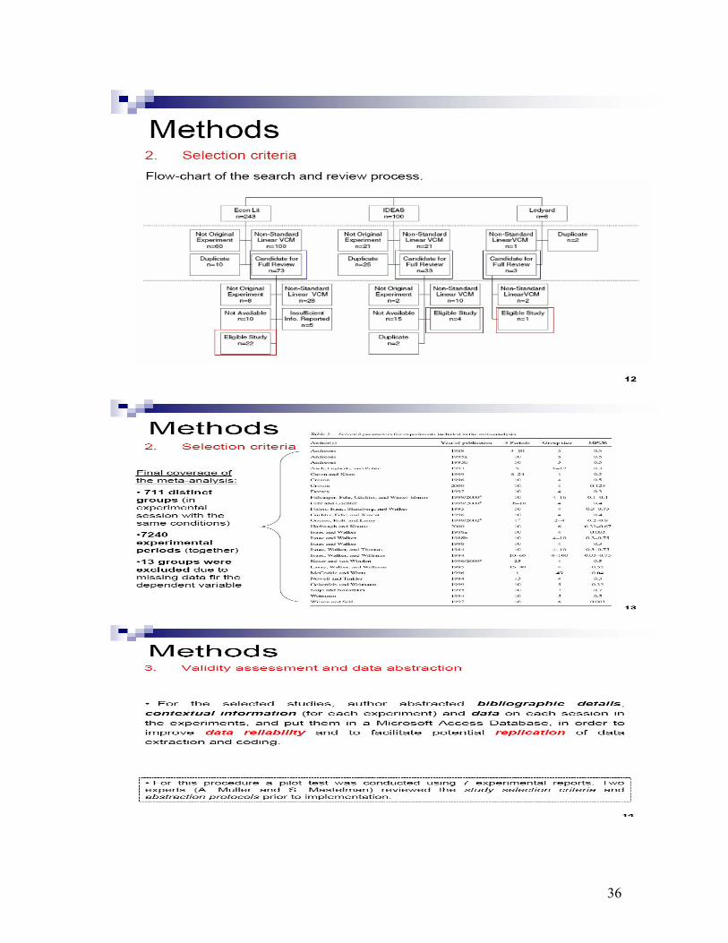
35

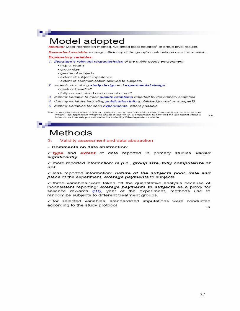
36

37

38

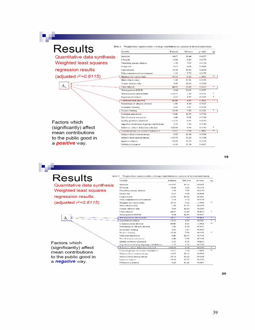
39

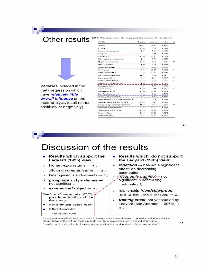
40

41

On with the show ☺

This is a chapter in Cherry et al (2008), Environmental Economics, Experimental Methods, Routlege.

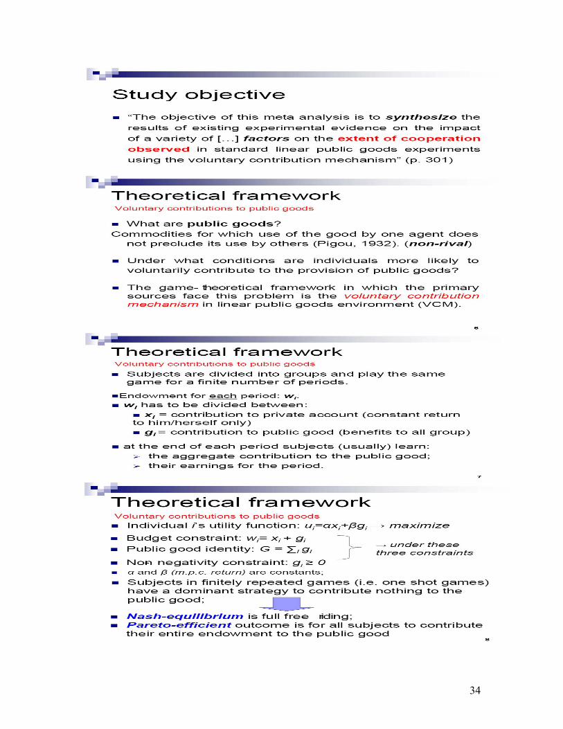
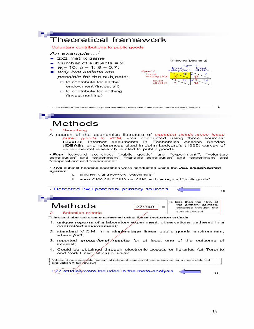
- VCM (= voluntary contributions mechanism) is the cornerstone of experimental investigations on the private provision of public goods

- Standard experimental investigation places individuals in a context-free setting where the public good, which is non-rival and non-excludable in consumption, simply money

- Specifically, “tokens” have to be divided between a private and a public account

- Typically, parameterized/designed so that each player has a dominant strategy of not contributing (to the public account)

- In one-shot (single-round) VCM experiments, subjects contribute – contrary to the theoretical prediction – about 40% - 60 %

- In finitely-repeated VCM experiments, subjects contribute about the same initially but contributions then decline towards zero (but rarely ever zero)

42

- “Thus, there seem to be motives for contributing that outweigh the incentive to free ride” (CFV 194)

- Possible “motives”: “pure altruism”, “warm-glow” (also called, “impure altruism”), “conditional cooperation”, “confusion”

- “Confusion” describes individuals’ failure to identify (in the laboratory set-up) the dominant strategy of no contribution (a realistic concern, see Rydval, Ortmann, Ostatnicky, Three Simple Games and How to Solve Them, now forthcoming in Journal of Economic Behavior and Organization: http://www.cerge-ei.cz/pdf/wp/Wp347.pdf

- Findings: o Palfrey & Prisbey (AER 1997) - find warm-glow but no evidence of

pure altruism o Goeree et al. (JPublE 2002) - find pure altruism but no warm-glow o Fischbacher et al. (EL 2001) – find conditional cooperation but no

pure / impure altruism, as do Fischbacher & Gaechter (manuscript 2004)

o etc. (contradictory gender effects, but see Ortmann & Tichy JEBO 1999)

o apparent lack of correspondence between contributions behavior in experimental and naturally occurring settings (e.g., Laury & Taylor JEBO 2008)

- Could it be that these findings are the result of confusion that “confounds” the interpretation of behavior in public good experiments? (p. 195)

o One new experiment, two old ones o Using the “virtual-player” method to sort out pro-social motives such

as altruism … - Finding:

o “The level of confusion in all experiments is both substantial and troubling.” (p. 196)

o “The experiments provide evidence that confusion is a confounding factor in investigations that discriminate among motives for public contributions, … “ (p. 196)

- Solutions: o Increase monetary rewards in VCM experiments ! (inadequate

monetary rewards having been identified as potential cause of contributions provided out of confusion)

o Make sure instructions are understandable ! (poorly prepared instructions having been identified as possible source of confusion)

o Make sure, more generally, that subjects manage to identify the dominant strategy ! (the inability of subjects to decipher the dominant strategy having been identified as a possible source of confusion)

o “Our results call into question the standard, “context-free” instructions used in public good games.” (p. 208)

43

In more detail:

- Andreoni (AER 1995) first to argue that (parts of) what looks like kindness in VCM experiments is really confusion. Andreoni finds that other-regarding behavior (kindness, altruism) and confusion are “equally important”

- Houser & Kurzban (AER 2oo2) did the same thing but they used a different set-up: - a “human condition” (the standard VCM game) - a “computer condition” (the standard VCM game, played by one

human player and three non-human (or, “virtual”) players. - Each round, the aggregate computer contribution to the public good

is three-quarters of the average contribution observed for that round in the human condition.

- Basic idea: confusion and other=regarding behavior present in the human condition but not in the computer condition

- Basic result: Confusion accounts for about 54 percent of contributions to all public good contributions.

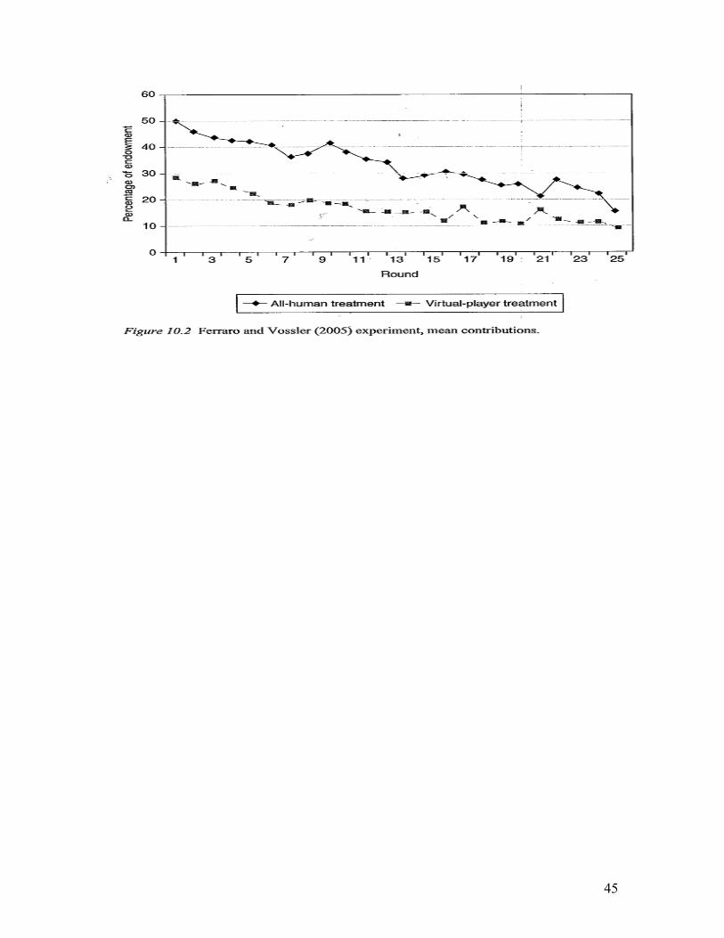
- Ferraro et al. (JEBO 2003) and Ferraro & Vossler (manuscript 2005), with designs similar to Houser & Kurzban find that 54 and 52 percent contributions come from confused subjects.

- Palfrey & Prisbey (1997) find a similar result in their own experiment (not using virtual players) and estimate with their model that “well over half” of the contributions in the classic VCM experiments by Isaac et al. (Public Choice 1984) are attributable to error.

- Goeree et al. (JPublE 2002) find in their own experiment (not using virtual players) both a positive and significant effect on coefficients that correspond to (pure) altruism and decision error (confusion); no point estimate is given,

- Fischbacher & Gaechter (manuscript 2004) find in their own experiment (not using virtual players) that “at most 17.5% “ are contributed by confused subjects; they also argue that none of their subjects exhibits altruism or warm-glow (no subject stated they would contribute if other group members would not). In Fischbacher & Gaechter’s view, all non-confused subjects are “conditional cooperators”

- Summary: every study that looks for confusion finds that it plays a significant role in observed contributions.

44

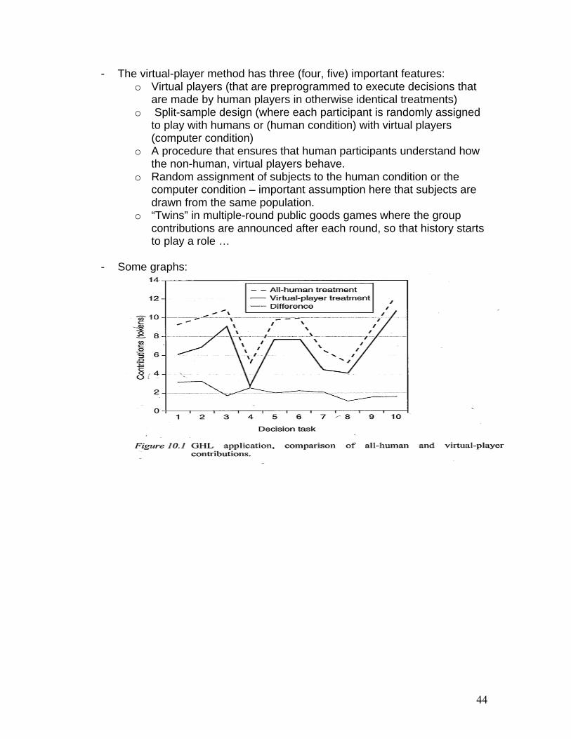
- The virtual-player method has three (four, five) important features: o Virtual players (that are preprogrammed to execute decisions that

are made by human players in otherwise identical treatments) o Split-sample design (where each participant is randomly assigned

to play with humans or (human condition) with virtual players (computer condition)

o A procedure that ensures that human participants understand how the non-human, virtual players behave.

o Random assignment of subjects to the human condition or the computer condition – important assumption here that subjects are drawn from the same population.

o “Twins” in multiple-round public goods games where the group contributions are announced after each round, so that history starts to play a role …

- Some graphs:

45