Embed Size (px)
Citation preview

Number Name of Table
Table WA1 Experimental questions and individual characteristics (female and male; full results)
Table WA2 Time discounting and financial behavior (female and male; means and standard deviations)
Table WA3 Time inconsistent preferences and SHG borrowing (female and male; full results)
Table WA4 Time inconsistent preferences and borrowing (female and male; full results)
Table WA5 Time inconsistent preferences and saving (female and male; full results)
Table WA6 Definition of variables (whole sample)
Table WA7 Correlations between experimental questions and gender, age, education and wealth (whole sample, female and male)
Table WA8 Time inconsistent preferences and SHG borrowing (alternative specification)
Table WA9 Time inconsistent preferences and borrowing (alternative specification)
Table WA10 Time inconsistent preferences and saving (alternative specification)
Table WA11 Time inconsistent preferences and home savings (robustness checks)
Table WA12 Time inconsistent preferences and SHG borrowing (non-linear discount rate)
Table WA13 Time inconsistent preferences and borrowing (non-linear discount rate)
Table WA14 Time inconsistent preferences and saving (non-linear discount rate)
Table WA15 Time inconsistent preferences and financial behavior (female; sub-sample analysis across levels of discount rates)
Table WA16 Time inconsistent preferences and SHG borrowing (strongly and weakly hyperbolic pooled)
Table WA17 Time inconsistent preferences and borrowing (strongly and weakly hyperbolics pooled)
Table WA18 Time inconsistent preferences and saving (strongly and weakly hyperbolics pooled)
Table WA19 Time inconsistent preferences and total savings without SHG savings
Table WA20 Time inconsistent preferences and SHG savings
Table WA21 Time inconsistent preferences and financial behavior (only female, farmers excluded)
Table WA22 Determinants of time preference reversals (farmers not controlled for)
Table WA23 Determinants of time preference reversals (negative shock from harvest not controlled for)
Table WA24 Determinants of discount rates (ordered probit)
Table WA25 Time inconsistent preferences and SHG borrowing (controlling for total savings)
Table WA26 Time inconsistent preferences and borrowing (controlling for total savings)
Behavioral Foundations of Microcredit: Experimental and Survey Evidence from Rural India
Michal Bauer, Julie Chytilová and Jonathan Morduch
SUPPLEMENTARY TABLES
APPENDIX - FOR ONLINE PUBLICATION ONLY

Table WA1: Experimental questions and individual characteristics (female and male; full results)
Dependent variable: Current discount rate Future discount rate Strongly present-biased Weakly present-biased
(1) (2) (3) (4) (5) (6) (7) (8) (9) (10)
female male female male female male female male female male
Gamble 2 -0.035 0.047 -0.019 -0.057 0.034 0.283 -0.038 -0.014 -0.030 -0.029
(0.058) (0.066) (0.057) (0.067) (0.121) (0.222) (0.041) (0.114) (0.090) (0.075)
Gamble 3 -0.054 0.041 -0.017 -0.026 -0.078 0.200 -0.090 0.111 0.032 0.054
(0.050) (0.058) (0.049) (0.059) (0.085) (0.185) (0.036)** (0.138) (0.111) (0.095)
Gamble 4 -0.159 0.029 -0.085 -0.039 -0.082 0.137 -0.046 0.228 0.135 -0.004
(0.054)*** (0.063) (0.052) (0.064) (0.083) (0.189) (0.039) (0.189) (0.151) (0.081)
Gamble 5 -0.084 0.021 -0.047 -0.020 -0.079 0.258 -0.067 0.095 0.025 0.079
(0.054) (0.059) (0.053) (0.060) (0.084) (0.200) (0.032) (0.134) (0.115) (0.106)
Gamble 6 -0.097 0.029 -0.060 -0.042 -0.126 0.214 0.006 0.121 -0.109 0.048
(0.056)* (0.058) (0.054) (0.059) (0.072) (0.190) (0.066) (0.140) (0.060) (0.092)
Education -0.003 -0.012 -0.005 -0.020 -0.005 0.003 0.000 0.003 -0.009 -0.009
(0.004) (0.005)** (0.004) (0.005)*** (0.009) (0.009) (0.005) (0.008) (0.010) (0.007)
Age 0.003 -0.008 0.002 -0.016 -0.017 0.006 0.003 0.015 -0.011 0.005
(0.008) (0.010) (0.008) (0.010) (0.016) (0.018) (0.011) (0.016) (0.019) (0.015)
(Age)2
-0.000 0.000 -0.000 0.000 0.000 -0.000 -0.000 -0.000 0.000 -0.000
(0.000) (0.000) (0.000) (0.000) (0.000) (0.000) (0.000) (0.000) (0.000) (0.000)
Married 0.026 -0.003 0.013 0.079 0.099 -0.137 -0.043 -0.053 -0.103
(0.044) (0.060) (0.043) (0.061) (0.072) (0.139) (0.073) (0.112) (0.115)
Household head -0.015 -0.019 -0.036 -0.024 0.229 0.045 -0.002 -0.061 0.070
(0.056) (0.045) (0.055) (0.046) (0.167) (0.082) (0.072) (0.081) (0.050)
Wealth 0.011 0.004 0.008 0.006 -0.006 -0.013 -0.005 0.022 -0.036 0.001
(0.008) (0.009) (0.008) (0.010) (0.017) (0.018) (0.011) (0.014) (0.023) (0.014)
Relative income 0.009 -0.034 -0.009 -0.054 0.015 -0.037 0.035 0.067 -0.025 -0.075
(0.027) (0.030) (0.026) (0.031)* (0.054) (0.055) (0.038) (0.049) (0.054) (0.041)*
Farmer 0.028 -0.021 -0.010 -0.037 0.097 0.119 -0.082 -0.105 -0.176 0.022
(0.031) (0.039) (0.030) (0.040) (0.056) (0.059)* (0.055) (0.080) (0.098)* (0.045)
Negative shock from harvest -0.036 -0.005 0.010 0.010 -0.090 -0.090 0.046 0.094 -0.022 0.029
(0.029) (0.035) (0.029) (0.036) (0.056) (0.067) (0.047) (0.056)* (0.061) (0.050)
Observations 266 272 266 272 266 243 211 216 151 244
(Pseudo) R-squared 0.29 0.24 0.20 0.22 0.16 0.12 0.22 0.16 0.19 0.13
* significant at 10%
** significant at 5%
*** significant at 1%
In columns 7,8 the dependent variable "Weakly present-biased preferences" equals to one if the respondent chose the more delayed reward one binary choice later in
the current time frame than in the future time frame. In columns 9,10 the dependent variable "Patient now, impatient in the future" equals to one if the respondent
chose more delayed reward earlier in the current time frame than in the future time frame. Omitted dummy variable for risk aversion is "Gamble 1" (the most risk
averse choice). In Column 9 the variables "Married" and "Household head" dropped due to lack of variation.
Level of discounting Time preference reversals
Patient now, impatient
in the future
Notes: All specifications include village fixed effects. OLS in columns 1-4. Probit, marginal effects reported in columns 5-10. In columns 1-2 the dependent variable
is the "Current discount rate" calculated from the binary choices between amount next day and amount after three months. It has six values calculated as arithmetic
means of inferred ranges of discount rate. In columns 3-4 the dependent variable is the "Future discount rate" calculated from the binary choices between amount
after one year or amount after one year and three months. In column 5,6 the dependent variable "Strongly present-biased preferences" equals to one if the respondent
chose the more delayed reward two or more binary choices later in the current time frame than in the future time frame.

Table WA2: Time discounting and financial behavior (female and male; means and standard deviations)
All
Low High
Strongly
hyperbolic
Weakly
hyperbolic
Time
consistent
Patient now,
impatient in
future
Female
Borrowing
SHG loan 0.426 0.457 0.371 0.607 0.447 0.359 0.391
(0.495) (0.500) (0.486) (0.493) (0.504) (0.481) (0.499)
Non-SHG loan 0.281 0.318 0.217 0.321 0.263 0.294 0.130
(0.451) (0.467) (0.414) (0.471) (0.466) (0.457) (0.344)
SHG loana
0.665 0.664 0.667 0.791 0.708 0.579 0.818
(0.473) (0.474) (0.476) (0.412) (0.464) (0.496) (0.405)
Saving
Any savings 0.863 0.884 0.825 0.857 0.842 0.876 0.826
(0.345) (0.321) (0.382) (0.353) (0.370) (0.331) (0.388)
Total savings (Rs. th.) 2.016 2.198 1.691 1.636 2.069 2.305 0.936
(2.736) (2.646) (2.875) (1.788) (3.808) (2.849) (0.952)
Share of home savingsb
0.191 0.182 0.208 0.164 0.148 0.194 0.306
(0.303) (0.291) (0.326) (0.278) (0.260) (0.307) (0.388)
Male
Borrowing
SHG loan 0.139 0.163 0.110 0.173 0.059 0.157 0.069
(0.346) (0.371) (0.314) (0.382) (0.239) (0.365) (0.258)
Non-SHG loan 0.369 0.367 0.371 0.404 0.412 0.352 0.345
(0.483) (0.484) (0.485) (0.495) (0.500) (0.479) (0.484)
Saving
Any savings 0.836 0.884 0.780 0.827 0.794 0.855 0.793
(0.371) (0.321) (0.416) (0.382) (0.410) (0.353) (0.412)
Total savings (Rs. th.) 3.113 3.350 2.839 3.221 3.206 3.267 1.967
(7.154) (6.375) (7.979) (5.148) (5.093) (8.539) (2.682)
Share of home savingsb
0.479 0.442 0.527 0.440 0.375 0.500 0.546
(0.407) (0.399) (0.415) (0.432) (0.353) (0.414) (0.376)
a The sample is restricted to only those who have any outstanding loan ("Loan"=1).
b The sample is restricted to only those who report having financial savings ("Any savings"=1).
Time consistencyFuture discount rate
Note: The variable "SHG loan" equals to one, if an individual has an outstanding loan from SHG. The variable "Non-SHG loan" equals to one, if an individual
has an outstanding loan from a bank, NGO or a moneylender. The variable "Any savings" equals to if a respondent reports any financial savings. "Total savings
(in thousands of Rs.)" are calculated as a sum of savings on a bank account, in a post office, contributions to SHGs and financial savings held at home. "Share
of home savings" is equal to financial home savings divided by "Total savings".

Table WA3: Time inconsistent preferences and SHG borrowing (female and male; full results)
Estimator
Dependent variable:
Conditioned by:
(1) (2) (3) (4) (5) (6) (7) (8) (9) (10) (11) (12)
female male female male female male female male female male female male
Strongly present-biased 0.277*** 0.0758 -0.00916 0.0616 0.401*** 0.0517 0.216** 0.0235 0.0522 0.0671 0.000855 0.164
(0.0732) (0.0800) (0.109) (0.0825) (0.0981) (0.0499) (0.107) (0.0444) (0.0846) (0.0947) (0.0783) (0.105)
Weakly present-biased -0.0461 -0.0581 -0.136 -0.0485 0.0500 -0.0610*** -0.00918 -0.0619*** -0.0790 0.130 -0.0916 0.166
(0.125) (0.0671) (0.133) (0.0719) (0.130) (0.0222) (0.128) (0.0226) (0.0859) (0.112) (0.0821) (0.116)
Patient now, impatient in the future -0.0748 -0.0879 0.132 -0.0749 0.0512 -0.0533** 0.180 -0.0453 -0.172*** 0.0698 -0.160*** -0.00546
(0.140) (0.0647) (0.109) (0.0695) (0.152) (0.0246) (0.155) (0.0305) (0.0566) (0.123) (0.0620) (0.116)
Current discount rate -0.911*** -0.113 -0.514** -0.0828 -0.191 0.181
(0.239) (0.122) (0.252) (0.0633) (0.169) (0.168)
Future discount rate -1.110*** 0.0135 -0.738*** -0.0395 -0.101 0.305*
(0.253) (0.128) (0.272) (0.0679) (0.175) (0.176)
Gamble 2 -0.220 0.145 -0.205 0.136 -0.292** 0.0598 -0.301** 0.0548 0.159 0.155 0.158 0.171
(0.203) (0.162) (0.206) (0.160) (0.137) (0.101) (0.135) (0.0991) (0.173) (0.166) (0.173) (0.167)
Gamble 3 -0.0119 0.104 -0.0311 0.0964 -0.0289 0.0276 -0.0622 0.0227 0.00559 0.158 0.00145 0.168
(0.152) (0.129) (0.156) (0.128) (0.168) (0.0730) (0.169) (0.0720) (0.127) (0.144) (0.126) (0.144)
Gamble 4 -0.453*** 0.00897 -0.463*** 0.00602 -0.181 -0.0135 -0.204 -0.0150 -0.00583 0.174 0.00580 0.187
(0.168) (0.123) (0.166) (0.122) (0.163) (0.0598) (0.160) (0.0602) (0.134) (0.158) (0.135) (0.159)
Gamble 5 -0.257 0.0756 -0.289 0.0713 -0.179 0.00105 -0.204 -0.000573 0.0684 -0.00855 0.0695 -0.00524
(0.180) (0.131) (0.181) (0.130) (0.160) (0.0679) (0.157) (0.0681) (0.145) (0.142) (0.145) (0.143)
Gamble 6 -0.0616 0.0317 -0.0932 0.0275 0.0400 0.0359 0.0101 0.0334 0.00939 -0.149 0.0119 -0.142
(0.180) (0.117) (0.186) (0.117) (0.191) (0.0796) (0.191) (0.0798) (0.137) (0.124) (0.137) (0.126)
Education -0.0192 0.0281*** -0.0214 0.0295*** -0.0179 0.00955* -0.0192 0.0101* -0.00159 0.00519 -0.00131 0.00804
(0.0134) (0.00889) (0.0135) (0.00891) (0.0140) (0.00545) (0.0141) (0.00561) (0.0103) (0.0117) (0.0103) (0.0119)
Age 0.0924*** -0.00229 0.0884*** -0.000874 0.0975*** 0.00501 0.0960*** 0.00544 0.0351* 0.0118 0.0343* 0.0145
(0.0262) (0.0179) (0.0264) (0.0180) (0.0272) (0.00973) (0.0274) (0.00999) (0.0204) (0.0231) (0.0204) (0.0232)
(Age)2
-0.00114*** -2.32e-05 -0.00112*** -4.02e-05 -0.00118*** -7.11e-05 -0.00117*** -7.64e-05 -0.000454* -0.000132 -0.000447* -0.000161
(0.000325) (0.000206) (0.000327) (0.000207) (0.000335) (0.000113) (0.000337) (0.000116) (0.000254) (0.000252) (0.000254) (0.000253)
Married 0.201 0.196*** 0.223 0.196*** 0.278* 0.0328 0.294** 0.0363 0.253*** 0.267*** 0.250*** 0.256**
(0.177) (0.0533) (0.180) (0.0533) (0.145) (0.0394) (0.143) (0.0388) (0.0630) (0.101) (0.0635) (0.103)
Household head -0.0481 -0.0628 -0.0193 -0.0628 0.103 -0.0269 0.135 -0.0293 0.104 -0.138 0.111 -0.133
(0.185) (0.0831) (0.185) (0.0825) (0.198) (0.0500) (0.200) (0.0510) (0.173) (0.108) (0.172) (0.108)
Wealth 0.0325 0.00355 0.0340 0.00170 -0.00495 0.00466 -0.00214 0.00411 0.0302 0.0182 0.0277 0.0168
(0.0268) (0.0169) (0.0270) (0.0168) (0.0288) (0.00890) (0.0290) (0.00902) (0.0204) (0.0222) (0.0202) (0.0222)
Relative income 0.00154 0.0492 0.0176 0.0533 -0.0124 0.0448 -0.0123 0.0453 -0.0478 0.000217 -0.0460 0.00913
(0.0816) (0.0534) (0.0836) (0.0536) (0.0872) (0.0293) (0.0882) (0.0299) (0.0624) (0.0703) (0.0622) (0.0706)
Farmer 0.130 -0.0756 0.122 -0.0707 -0.0574 -0.0576 -0.0660 -0.0562 0.169*** 0.0404 0.167** 0.0418
(0.102) (0.0830) (0.102) (0.0826) (0.0984) (0.0543) (0.0986) (0.0544) (0.0652) (0.0945) (0.0653) (0.0946)
Negative shock from harvest 0.0265 0.0353 0.0619 0.0355 0.202** 0.00782 0.225** 0.00768 -0.113* 0.0820 -0.111* 0.0848
(0.0958) (0.0641) (0.0959) (0.0642) (0.0959) (0.0342) (0.0963) (0.0347) (0.0651) (0.0830) (0.0655) (0.0831)
Position 0.201*** 0.219*** 0.254*** 0.265*** -0.0635 -0.0643
(0.0774) (0.0807) (0.0889) (0.0904) (0.0612) (0.0614)
(Position)2
-0.0230** -0.0239** -0.0238** -0.0245** 0.00846 0.00858
(0.0106) (0.0110) (0.0119) (0.0121) (0.00835) (0.00837)
Observations 239 261 239 261 232 250 232 250 249 272 249 272
* significant at 10%
** significant at 5%
*** significant at 1%
Notes: In all specifications we control for risk aversion (six dummies corresponding to chosen gamble), observable characteristics (education, age, married, household head, wealth, relative income, farmer, negative shock from
harvest; for women we also control for their position within household) and village fixed effects. The dependent variable in columns 1-4 is "SHG participation" and it equals to one, if an individual is a member of a self-help group
(SHG). The dependent variable in columns 5-8 is "SHG borrowing" and it equals to one if an individual has an outstanding loan from SHG. The dependent variable in columns 9-12 is "Non-SHG borrowing" and it equals to one if an
individual has an outstanding loan from a bank or a moneylender.
Current discount rate Future discount rate Current discount rate Future discount rate Current discount rate Future discount rate
Probit Probit Probit
SHG participation SHG borrowing Non-SHG borrowing

Table WA4: Time inconsistent preferences and borrowing (female and male; full results)
Estimator
Dependent variable:
Conditioned by:
(5) (6) (7) (8) (1) (2) (3) (4)
female male female male female male female male
Strongly present-biased 0.318*** 0.0109 0.253*** -0.0403 0.0600 0.0877 -0.0636 0.111
(0.0800) (0.0881) (0.0932) (0.0838) (0.140) (0.116) (0.150) (0.125)
Weakly present-biased 0.0138 -0.180*** -0.0214 -0.184*** -0.0482 0.139 -0.0990 0.138
(0.161) (0.0510) (0.167) (0.0510) (0.190) (0.140) (0.191) (0.143)
Patient now, impatient in the future 0.225** -0.129** 0.238*** -0.107 0.257** 0.0901 0.275** 0.0621
(0.0915) (0.0554) (0.0812) (0.0738) (0.130) (0.169) (0.119) (0.177)
Current discount rate -0.303 -0.190 -0.424 0.113
(0.328) (0.153) (0.338) (0.233)
Future discount rate -0.375 -0.146 -0.380 0.0735
(0.366) (0.165) (0.401) (0.242)
Gamble 2 -0.0841 0.164 -0.121 0.146 0.0564 0.192 0.0634 0.199
(0.287) (0.222) (0.298) (0.219) (0.214) (0.177) (0.212) (0.174)
Gamble 3 0.291* 0.0905 0.275 0.0751 0.386*** 0.196 0.374*** 0.207
(0.164) (0.168) (0.169) (0.165) (0.129) (0.172) (0.133) (0.169)
Gamble 4 0.234 0.0500 0.220 0.0483 0.445*** 0.0693 0.449*** 0.0774
(0.150) (0.186) (0.159) (0.188) (0.0636) (0.205) (0.0632) (0.203)
Gamble 5 0.189 0.152 0.180 0.151 0.244* -0.0148 0.244* -0.00783
(0.154) (0.225) (0.159) (0.226) (0.146) (0.201) (0.146) (0.200)
Gamble 6 0.244* 0.358 0.232 0.341 0.433*** 0.129 0.431*** 0.141
(0.140) (0.252) (0.148) (0.252) (0.0901) (0.189) (0.0922) (0.184)
Education -0.00374 0.0188 -0.00628 0.0200 -0.0245 0.0160 -0.0266 0.0152
(0.0183) (0.0126) (0.0187) (0.0128) (0.0221) (0.0168) (0.0222) (0.0168)
Age 0.0772** -0.000982 0.0799** -0.00189 0.0353 0.0380 0.0324 0.0388
(0.0346) (0.0225) (0.0348) (0.0228) (0.0408) (0.0345) (0.0408) (0.0345)
(Age)2
-0.000906** 3.51e-05 -0.000940** 4.40e-05 -0.000636 -0.000471 -0.000609 -0.000479
(0.000422) (0.000246) (0.000424) (0.000249) (0.000494) (0.000378) (0.000495) (0.000378)
Married 0.190 -0.0260 0.195 -0.0129 0.634*** -0.0365 0.621*** -0.0416
(0.292) (0.139) (0.292) (0.135) (0.202) (0.198) (0.209) (0.198)
Household head -0.00497 -0.0625 0.0185 -0.0627 0.337*** -0.0237 0.343*** -0.0256
(0.246) (0.120) (0.240) (0.120) (0.116) (0.156) (0.115) (0.156)
Wealth -0.00331 0.00850 -0.00128 0.00814 0.120** -0.0291 0.116** -0.0281
(0.0394) (0.0223) (0.0399) (0.0226) (0.0500) (0.0326) (0.0500) (0.0324)
Relative income -0.0953 0.0724 -0.0902 0.0716 -0.0794 0.155 -0.0707 0.152
(0.107) (0.0696) (0.107) (0.0712) (0.126) (0.0989) (0.126) (0.0995)
Farmer -0.233** -0.258 -0.237** -0.252 -0.129 0.284* -0.141 0.279*
(0.108) (0.180) (0.106) (0.179) (0.145) (0.155) (0.142) (0.155)
Negative shock from harvest 0.278*** 0.0150 0.283*** 0.0102 0.109 -0.0405 0.126 -0.0353
(0.104) (0.0913) (0.104) (0.0921) (0.123) (0.123) (0.120) (0.122)
Position 0.252** 0.255** 0.395** 0.374**
(0.121) (0.121) (0.161) (0.157)
(Position)2
-0.0222 -0.0226 -0.0375* -0.0353*
(0.0161) (0.0161) (0.0202) (0.0198)
Observations 139 140 139 140 130 151 130 151
* significant at 10%
** significant at 5%
*** significant at 1%
Notes: In all specifications we control for risk aversion (six dummies corresponding to chosen gamble), observable characteristics (education, age, married, household
head, wealth, relative income, farmer, negative shock from harvest; for women we also control for their position within household) and village fixed effects. The
dependent variable in columns 1-4 is "SHG borrowing" "SHG borrowing" and it equals to one if an individual has an outstanding loan from SHG. The dependent
variable in columns 5-8 is "Delayed repayment of outstanding loan" and it equals to one if an individual has been delayed on repayment of the outstanding loan for at
least one installment.
ProbitProbit
Delayed repayment of outstanding loan
Current discount rate Future discount rateCurrent discount rate Future discount rate
SHG borrowing

Table WA5: Time inconsistent preferences and saving (female and male; full results)
Estimator
Dependent variable:
Conditioned by:
(1) (2) (3) (4) (5) (6) (7) (8)
female male female male female male female male
Strongly present-biased -0.277 0.641 -0.839* 0.0588 -0.179** -0.132 0.0155 -0.0345
(0.450) (1.123) (0.442) (1.189) (0.0885) (0.125) (0.0825) (0.126)
Weakly present-biased -0.202 -0.634 -0.363 -1.003 0.0373 -0.0437 0.0953 -0.00808
(0.535) (1.321) (0.535) (1.351) (0.101) (0.144) (0.101) (0.146)
Patient now, impatient in the future -1.279** -0.257 -0.892 0.144 0.230** 0.102 0.109 0.0165
(0.605) (1.402) (0.611) (1.377) (0.107) (0.150) (0.111) (0.150)
Current discount rate -1.438 -0.462 0.603*** 0.181
(0.920) (2.041) (0.167) (0.225)
Future discount rate -2.032** -2.294 0.500*** 0.358
(0.952) (2.109) (0.176) (0.228)
Gamble 2 0.0628 3.765** 0.0818 3.700** 0.245* -0.146 0.241* -0.121
(0.765) (1.874) (0.761) (1.869) (0.142) (0.213) (0.144) (0.213)
Gamble 3 0.663 1.113 0.622 1.092 0.203* -0.119 0.217* -0.105
(0.654) (1.664) (0.651) (1.658) (0.122) (0.191) (0.124) (0.190)
Gamble 4 -0.162 0.459 -0.175 0.441 0.340** -0.0300 0.319** -0.0184
(0.715) (1.798) (0.707) (1.792) (0.134) (0.202) (0.136) (0.201)
Gamble 5 0.779 0.0189 0.726 0.0303 0.317** -0.0818 0.331** -0.0723
(0.713) (1.705) (0.711) (1.701) (0.133) (0.192) (0.135) (0.191)
Gamble 6 1.123 1.416 1.084 1.378 0.302** -0.0644 0.296** -0.0502
(0.734) (1.670) (0.731) (1.665) (0.132) (0.192) (0.134) (0.191)
Education -0.0702 0.294** -0.0763 0.260* 0.0158 -0.0291* 0.0163 -0.0259*
(0.0575) (0.142) (0.0574) (0.144) (0.0102) (0.0152) (0.0103) (0.0152)
Age 0.256** 0.403 0.249** 0.377 -0.0233 0.0286 -0.0233 0.0318
(0.106) (0.278) (0.105) (0.278) (0.0192) (0.0311) (0.0193) (0.0310)
(Age)2
-0.00317** -0.00446 -0.00313** -0.00419 0.000241 -0.000303 0.000253 -0.000337
(0.00131) (0.00306) (0.00130) (0.00306) (0.000241) (0.000349) (0.000243) (0.000348)
Married -0.0234 4.070** -0.0131 4.202** 0.382*** -0.586*** 0.380*** -0.605***
(0.638) (1.716) (0.635) (1.715) (0.116) (0.184) (0.117) (0.183)
Household head 0.234 -5.714*** 0.273 -5.782*** 0.427*** 0.0512 0.402*** 0.0601
(0.800) (1.293) (0.795) (1.291) (0.143) (0.138) (0.144) (0.137)
Wealth 0.416*** 1.129*** 0.415*** 1.145*** 0.0264 -0.0757*** 0.0295 -0.0770***
(0.111) (0.268) (0.110) (0.267) (0.0191) (0.0291) (0.0193) (0.0289)
Relative income -0.181 -0.146 -0.181 -0.236 0.154** 0.00658 0.154** 0.0164
(0.354) (0.864) (0.353) (0.864) (0.0627) (0.0937) (0.0634) (0.0933)
Farmer 0.0730 -0.350 0.0623 -0.405 0.129* 0.185 0.133* 0.194
(0.416) (1.124) (0.414) (1.120) (0.0746) (0.124) (0.0751) (0.124)
Negative shock from harvest 0.0258 -1.307 0.0693 -1.300 -0.197*** -0.0466 -0.214*** -0.0432
(0.391) (1.009) (0.389) (1.006) (0.0718) (0.114) (0.0726) (0.114)
Position 0.0239 0.0317 0.0215 0.0144
(0.347) (0.345) (0.0653) (0.0663)
(Position)2
-0.00732 -0.00664 0.00138 0.00188
(0.0466) (0.0464) (0.00851) (0.00863)
Observations 249 272 249 272 213 227 213 227
R-squared 0.256 0.329 0.263 0.332
a The sample is restricted to only those who report having positive financial savings ("Total savings">0).
* significant at 10%
** significant at 5%
*** significant at 1%
Notes: In all specifications we control for risk aversion (six dummies corresponding to chosen gamble), observable characteristics (education, age, married, household
head, wealth, relative income, farmer, negative shock from harvest; for women we also control for their position within household) and village fixed effects. The
dependent variable in columns 1-4 are Total savings (in thousands of Rs.)" and it is calculated as a sum of savings on a bank account, in a post office, contributions to
SHGs and financial savings held at home. The dependent variable in columns 5-8 is "Share of home savings" and it is equal to financial home savings divided by "Total
savings".
OLS
Total savings (Rs. th.)
Current discount rate Future discount rate
Tobit
Share of home savingsa
Current discount rate Future discount rate

Table WA6: Definition of variables (whole sample)
Variables Definition Mean Std dev
Experimental choice s
6 values approximating 3-months discount rate in earlier time frame:
0.03 = if discount rate < 6%; 0.09= if 6% < discount rate < 12%; 0.16 if 12%
< discount rate < 20%; 0.26 = if 20% < discount rate < 32%, 0.14 if 32% <
discount rate < 50%; 0.6= if 50% < discount rate
6 values approximating 3-months discount rate in delayed time frame:
0.03 = if discount rate < 6%; 0.09= if 6% < discount rate < 12%; 0.16 if 12%
< discount rate < 20%; 0.26 = if 20% < discount rate < 32%, 0.14 if 32% <
discount rate < 50%; 0.6= if 50% < discount rate
Strongly present-biased dummy; 1= current discount rate >> future discount rate, the future income
option is chosen at least two rows later in the current time frame than in the
future time frame
0.199 0.399
Weakly present-biased dummy; 1= current discount rate > future discount rate, the future income
option is chosen one row later in the current time frame than in the future time
frame
0.132 0.339
Patient now, impatient in the future dummy, 1= current discount rate < future discount rate 0.096 0.294
Attitude to risk set of dummies, one for each of the following gambles: (250,250); (225,475);
(200,600); (150,750); (50,950); (0,1000). In this table the mean is for first
gamble=1, second gamble=2, …, sixth gamble=6.
3.844 1.538
Financial behavior
SHG participation Dummy; 1 = being a member of a self-help group (SHG); 0 = not being a
member of a SHG
0.427 0.495
SHG borrowing Dummy; 1 = has an outstanding loan from SHG; 0 = doesn’t have an
outstanding loan from SHG
0.281 0.450
Non-SHG borrowing Dummy; 1 = has an outstanding loan from a bank or a moneylender; 0 =
doesn’t have an outstanding loan from a bank or a moneylender
0.325 0.469
Delayed repayment of outstanding loan Dummy; 1 = being delayed on repayment of the outstanding loan for at least
one installment; 0 = never delayed on repayment
0.628 0.484
Total savings Rs. th. (savings in bank + savings in post office + SHG monthly
contribution*average length of participation + home savings)
2.569 5.454
Savings in bank Rs. th. 1.127 3.808
Savings in post office Rs. th. 0.441 2.523
SHG savings Rs. th. (SHG monthly contribution*average length of participation) 0.431 0.606
Home savings Rs. th. 0.570 1.606
Share of home savings Home savings /Total savings (%, only those who save) 0.333 0.386
Future oriented purpose of savings Dummy; 1 = if the major purpose of savings is future-oriented (agricultural
investment, business, education, doctor); 0 = if it focuses on current
consumption (celebration, personal items, household equipment)
0.546 0.498
Socioeconomic characteristics
Female Dummy; 1 = female; 0 = male 0.496 0.500
Age Age in years 36.822 11.756
Education Years of schooling completed 4.256 4.442
Married Dummy; 1 = married; 0 = single or widow 0.786 0.410
Household head Dummy; 1 = household head; 0 = non household head 0.397 0.490
Wealth index Wealth index calculated by principal component analyses from questions on
type of house, electricity connection, land ownership and dummies for
possesion of 14 types of household equipment
0.000 1.893
Relative income Dummy; 1 = if income in June < income in September; 0 = if income in June
>= income in September
0.496 0.500
Farmer Dummy; 1 = farmer; 0 = non farmer 0.702 0.458
Negative shock from harvest Dummy; 1 = bad harvest reported as the major negative shock in the past five
years0.423 0.494
Current discount rate 0.244 0.228
Future discount rate 0.193 0.221

Table WA7: Correlations between experimental questions and gender, age, education and wealth (whole sample, female and male)
Current discount
rate Future discount rate
Strongly present-
biased
Weakly present-
biased
Patient now,
impatient in the
future
Whole sample
Sex -0.114* -0.150* 0.022 0.025 -0.035
(0.008) (0.000) (0.607) (0.567) (0.414)
Education -0.222* -0.224* -0.043 0.050 -0.023
(0.000) (0.000) (0.315) (0.248) (0.593)
Wealth -0.122* -0.126* -0.047 0.065 -0.063
(0.004) (0.003) (0.272) (0.130) (0.143)
Female
Education -0.127 -0.121 -0.052 -0.002 -0.060
(0.037) (0.047) (0.399) (0.971) (0.323)
Wealth -0.040 -0.060 -0.047 0.026 -0.126
(0.509) (0.325) (0.446) (0.666) (0.040)
Male
Education -0.337* -0.349* -0.030 0.106 -0.005
(0.000) (0.000) (0.618) (0.079) (0.930)
Wealth -0.199* -0.188* -0.046 0.105 -0.014
(0.001) (0.002) (0.444) (0.083) (0.821)
* significant at 1%
p-values in parentheses

Comparison of specifications in this paper and in Ashraf, Karlan and Yin (2006)
Ashraf et al. (2006) apply the following specification: (2)
Table WA8: Time inconsistent preferences and SHG borrowing (alternative specification)
Estimator
Dependent variable:
(1) (2) (3) (4) (5) (6)
female male female male female male
Strongly hyperbolic 0.209 -0.051 0.323 -0.038 0.378 -0.123
(0.109) (0.094) (0.119)*** (0.059) (0.096)*** (0.113)
Weakly hyperbolic -0.036 -0.119 0.053 -0.074 0.172 -0.179
(0.101) (0.070) (0.125) (0.042) (0.090) (0.071)*
Current discount rate==.09 0.027 0.047 0.044 -0.107 -0.045 -0.190
(0.101) (0.121) (0.147) (0.033)** (0.177) (0.075)**
Current discount rate==.16 -0.075 0.131 -0.051 0.043 -0.285 0.059
(0.145) (0.140) (0.156) (0.091) (0.157)* (0.141)
Current discount rate==.26 -0.225 0.315 -0.196 0.140 -0.230 0.183
(0.161) (0.176)** (0.150) (0.125) (0.230) (0.204)
The next Tables WA8-WA10 show our results using the specification of Ashraf et al. (2006)
Ashfaf et al. use a related specification in their analysis of a commitment savings product—with a slightly different
interpretation. To see the difference, consider the case when there are only two values of each discount rate – high and
low. There are then four types of individuals: patient and time consistent, impatient and time consistent, hyperbolic
(current discount rate high, future discount rate low), and time inconsistent with a future bias (current discount rate
low, future discount rate high).
The coefficient α3 estimates the effect of being hyperbolic relative to time consistent or future biased individuals
(here, it is not possible to also identify the coefficient on the dummy for being future-biased). A comparable version
of our specification (1) can be written as where t=0,1.
The difference is that we include only one of the discount rates and add the dummy for future biased individuals.
When we control for current patience, the coefficient β'3 indicates a difference in behavior between the hyperbolic
group and the time consistent impatient group, and it can be shown that β'3=α3-α2 . In the second version, where we
control for future patience, the behavior of hyperbolic group is contrasted to the time consistent patient group and
β'3=α3-α2. Our specification generalizes this simple set-up.
In the paper we compare how the behavior of the hyperbolic individuals departs from that of time consistent
individuals, conditional on their level of patience. Two natural benchmarks arise: the level of patience associated with
current patience (current self) and the level associated with future patience (future self). In equation (1) our two
coefficients for hyperbolic preferences directly capture these departures, whereas the coefficient in Ashraf et al (2006)
compares hyperbolic individuals to the average behavior of the group of time consistent and future-biased individuals.
Probit Probit Probit
SHG participation SHG borrowing SHG borrowinga
0 1
0 1 2 3i i i i iY D D Hα α α α ε= + + + + +6 iα X
' ' ' '
0 1 3 4
t
i i i i iY D H Fβ β β β ε= + + + + +
'
6 iβ X
(0.161) (0.176)** (0.150) (0.125) (0.230) (0.204)
Current discount rate==.41 -0.639 -0.333 -0.659
(0.131)*** (0.082)** (0.086)***
Current discount rate==.60 -0.074 0.023 0.034 0.015 -0.255 0.052
(0.188) (0.139) (0.173) (0.100) (0.293) (0.198)
Future discount rate==.09 -0.226 -0.129 -0.114 -0.012 -0.132 -0.035
(0.112)** (0.072) (0.106) (0.055) (0.138) (0.111)
Future discount rate==.16 -0.173 -0.184 -0.101 -0.121 0.055 -0.217
(0.107)* (0.044)*** (0.128) (0.024)*** (0.185) (0.046)***
Future discount rate==.26 0.162 -0.061 0.192 -0.043 0.254 -0.026
(0.103) (0.087) (0.146) (0.062) (0.096)* (0.149)
Future discount rate==.41 0.119 0.364
(0.229) (0.239)
Future discount rate==.60 -0.464 -0.035 -0.318 -0.064 -0.050 -0.139
(0.161)*** (0.113) (0.105)** (0.062) (0.281) (0.139)
Conditional on borrowing? no no no no yes yes
Pseudo R-squared 0.28 0.14 0.25 0.11 0.19 0.15
Observations 249 260 249 261 157 148
a The sample is restricted to only those who have any outstanding loan ("Loan"=1)
* significant at 10%
** significant at 5%
*** significant at 1%
Notes: Table reports the coefficients after controlling for dummies for each level of current discount rate, dummies
for each level of future discount rate (as in Ashraf et al. 2006). Standard errors corrected for clustering at the village
level. In all columns we control for risk aversion (six dummies corresponding to chosen gamble), observable
characteristics (education, age, married, household head, wealth, relative income, farmer, negative shock from
harvest; for women we also control for their position within household). The dependent variable in columns 1-4 is
"SHG participation" and it equals to one, if an individual is a member of a self-help group (SHG). The dependent
variable in columns 5-12 is "SHG borrowing" and it equals to one if if an individual has an outstanding loan from
SHG.
0 1
0 1 2 3i i i i iY D D Hα α α α ε= + + + + +6 iα X
' ' ' '
0 1 3 4
t
i i i i iY D H Fβ β β β ε= + + + + +
'
6 iβ X
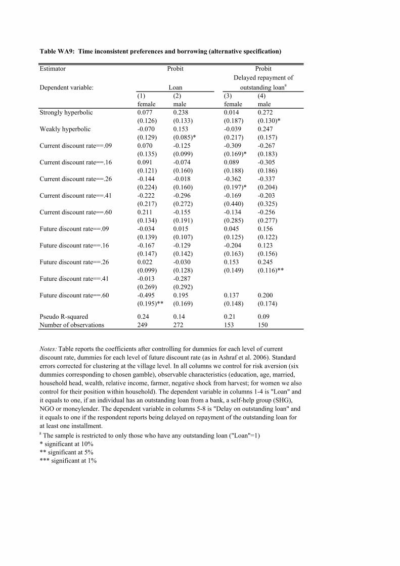
Table WA9: Time inconsistent preferences and borrowing (alternative specification)
Estimator
Dependent variable:
(1) (2) (3) (4)
female male female male
Strongly hyperbolic 0.077 0.238 0.014 0.272
(0.126) (0.133) (0.187) (0.130)*
Weakly hyperbolic -0.070 0.153 -0.039 0.247
(0.129) (0.085)* (0.217) (0.157)
Current discount rate==.09 0.070 -0.125 -0.309 -0.267
(0.135) (0.099) (0.169)* (0.183)
Current discount rate==.16 0.091 -0.074 0.089 -0.305
(0.121) (0.160) (0.188) (0.186)
Current discount rate==.26 -0.144 -0.018 -0.362 -0.337
(0.224) (0.160) (0.197)* (0.204)
Current discount rate==.41 -0.222 -0.296 -0.169 -0.203
(0.217) (0.272) (0.440) (0.325)
Current discount rate==.60 0.211 -0.155 -0.134 -0.256
(0.134) (0.191) (0.285) (0.277)
Future discount rate==.09 -0.034 0.015 0.045 0.156
(0.139) (0.107) (0.125) (0.122)
Future discount rate==.16 -0.167 -0.129 -0.204 0.123
(0.147) (0.142) (0.163) (0.156)
Future discount rate==.26 0.022 -0.030 0.153 0.245
(0.099) (0.128) (0.149) (0.116)**
Future discount rate==.41 -0.013 -0.287
(0.269) (0.292)
Future discount rate==.60 -0.495 0.195 0.137 0.200
(0.195)** (0.169) (0.148) (0.174)
Pseudo R-squared 0.24 0.14 0.21 0.09
Number of observations 249 272 153 150
a The sample is restricted to only those who have any outstanding loan ("Loan"=1)
* significant at 10%
** significant at 5%
*** significant at 1%
Notes:Table reports the coefficients after controlling for dummies for each level of current
discount rate, dummies for each level of future discount rate (as in Ashraf et al. 2006). Standard
errors corrected for clustering at the village level. In all columns we control for risk aversion (six
dummies corresponding to chosen gamble), observable characteristics (education, age, married,
household head, wealth, relative income, farmer, negative shock from harvest; for women we also
control for their position within household). The dependent variable in columns 1-4 is "Loan" and
it equals to one, if an individual has an outstanding loan from a bank, a self-help group (SHG),
NGO or moneylender. The dependent variable in columns 5-8 is "Delay on outstanding loan" and
it equals to one if the respondent reports being delayed on repayment of the outstanding loan for
at least one installment.
Probit
Delayed repayment of
outstanding loana
Loan
Probit

Table WA10: Time inconsistent preferences and saving (alternative specification)
Estimator
Dependent variable:
(1) (2) (3) (4) (5) (6)
female male female male female male
Strongly hyperbolic -1.463 -1.645 0.069 -0.028 -0.204 0.150
(0.630)** (1.369) (0.208) (0.157) (0.166) (0.151)
Weakly hyperbolic -1.068 -2.265 -0.013 -0.041 0.037 0.265
(0.940) (1.782) (0.128) (0.119) (0.097) (0.152)*
Current discount rate==.09 0.954 2.220 0.066 -0.029 -0.221 -0.338
(0.622) (1.837) (0.126) (0.135) (0.105)** (0.120)***
Current discount rate==.16 0.280 1.342 -0.081 -0.098 -0.125 -0.220
(0.703) (1.864) (0.185) (0.175) (0.164) (0.182)
Current discount rate==.26 1.438 1.795 -0.105 0.049 0.127 -0.461
(1.019) (2.239) (0.264) (0.149) (0.181) (0.289)
Current discount rate==.41 0.421 1.232 0.078 -0.278 0.153 -0.096
(1.013) (2.535) (0.320) (0.234) (0.333) (0.195)
Current discount rate==.60 1.254 2.933 -0.261 -0.339 0.138 -0.281
(0.748) (1.431)* (0.190) (0.134)** (0.236) (0.203)
Future discount rate==.09 -0.287 -2.295 -0.065 0.073 0.259 0.088
(0.381) (1.624) (0.125) (0.102) (0.114)** (0.187)
Future discount rate==.16 -0.295 0.524 -0.167 0.137 -0.068 0.065
(0.687) (1.034) (0.143) (0.190) (0.133) (0.172)
Future discount rate==.26 -0.667 -1.645 -0.313 -0.150 -0.146 -0.032
(0.992) (2.025) (0.169)* (0.141) (0.225) (0.358)
Future discount rate==.41 -2.227 -2.086 -0.084 0.285 -0.021 -0.401
(0.767)*** (2.101) (0.454) (0.201) (0.613) (0.182)**
Future discount rate==.60 -2.153 -3.226 -0.094 0.093 0.284 0.426
(0.927)** (1.516)** (0.201) (0.140) (0.233) (0.215)**
(Pseudo) R-squared 0.22 0.28 0.20 0.15 018 0.14
Number of observations 249 272 248 271 213 227
a The sample is restricted to only those who report having positive financial savings ("Total savings">0).
* significant at 10%
** significant at 5%
*** significant at 1%
The dependent variable in columns 9-12 "Future-oriented purpose of savings" is equal to one, if the major self-reported purpose of savings is
future-oriented (agricultural investment, business, education, doctor), and equal to zero, if it focuses on current consumption (celebration,
personal items, household equipment).
Future-oriented
purpose of savings
Notes: Table reports the coefficients after controlling for dummies for each level of current discount rate, dummies for each level of future
discount rate (as in Ashraf et al. 2006). Standard errors corrected for clustering at the village level. In all columns we control for risk aversion
(six dummies corresponding to chosen gamble), observable characteristics (education, age, married, household head, wealth, relative income,
farmer, negative shock from harvest; for women we also control for their position within household). The dependent variable in columns 1-4
are Total savings (in thousands of Rs.)" and it is calculated as a sum of savings on a bank account, in a post office, contributions to SHGs and
financial savings held at home. The dependent variable in columns 5-8 is "Share of home savings" and it is equal to financial home savings
divided by "Total savings".
Share of home savingsa
Tobit
Total savings (Rs. th.)
OLS Probit
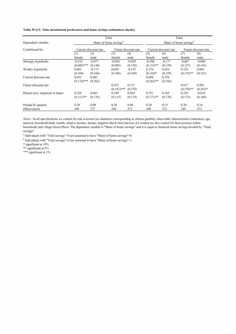
Table WA11: Time inconsistent preferences and home savings (robustness checks)
Dependent variable:
Conditioned by:
(1) (2) (3) (4) (5) (6) (7) (8)
female male female male female male female male
Strongly hyperbolic -0.232 -0.077 -0.036 -0.029 -0.280 -0.177 -0.067 -0.040
(0.088)*** (0.144) (0.085) (0.150) (0.133)** (0.139) (0.127) (0.143)
Weakly hyperbolic 0.003 -0.173 0.054 -0.153 0.276 0.010 0.325 0.065
(0.104) (0.166) (0.106) (0.169) (0.154)* (0.159) (0.155)** (0.161)
Current discount rate 0.652 0.082 0.608 0.238
(0.174)*** (0.262) (0.265)** (0.256)
Future discount rate 0.472 0.171 0.617 0.501
(0.181)*** (0.270) (0.270)** (0.263)*
Patient now, impatient in future 0.229 0.063 0.109 0.024 0.351 0.103 0.218 -0.010
(0.111)** (0.176) (0.115) (0.174) (0.171)** (0.170) (0.173) (0.168)
Pseudo R-squared 0.30 0.08 0.28 0.08 0.20 0.15 0.20 0.16
Observations 249 272 249 272 249 272 249 272
a Individuals with "Total savings"=0 are assumed to have "Share of home savings"=0.
b Individuals with "Total savings"=0 are assumed to have "Share of home savings"=1.
* significant at 10%
** significant at 5%
*** significant at 1%
Tobit
Share of home savingsb
Notes: In all specifications we control for risk aversion (six dummies corresponding to chosen gamble), observable characteristics (education, age,
married, household head, wealth, relative income, farmer, negative shock from harvest; for women we also control for their position within
household) and village fixed effects. The dependent variable is "Share of home savings" and it is equal to financial home savings divided by "Total
savings".
Tobit
Share of home savingsa
Current discount rate Future discount rate Current discount rate Future discount rate

Table WA12: Time inconsistent preferences and SHG borrowing (non-linear discount rate)
Estimator
Dependent variable:
Conditioned by:
(1) (2) (3) (4) (5) (6) (7) (8) (9) (10) (11) (12)
female male female male female male female male female male female male
Strongly hyperbolic 0.334 0.051 -0.032 0.048 0.460 0.056 0.217 0.015 0.319 0.046 0.205 -0.056
(0.067)*** (0.085) (0.115) (0.082) (0.099)*** (0.054) (0.109)* (0.042) (0.084)*** (0.109) (0.105)* (0.072)
Weakly hyperbolic 0.023 -0.086 -0.142 -0.052 0.055 -0.040 -0.081 -0.064 0.077 -0.136 -0.135 -0.175
(0.136) (0.072) (0.140) (0.074) (0.150) (0.035) (0.130) (0.022)* (0.161) (0.074) (0.210) (0.050)***
Current discount rate==.09 -0.011 0.018 0.096 -0.061 -0.024 -0.158
(0.140) (0.105) (0.150) (0.026) (0.196) (0.062)
Current discount rate==.16 -0.293 -0.002 -0.112 -0.036 -0.096 -0.106
(0.144)** (0.091) (0.132) (0.031) (0.202) (0.080)
Current discount rate==.26 -0.136 0.167 -0.156 -0.000 0.187 -0.073
(0.210) (0.153) (0.161) (0.055) (0.133) (0.096)
Current discount rate==.41 -0.684 -0.361 -0.428
(0.080)*** (0.105)*** (0.357)
Current discount rate==.60 -0.515 -0.057 -0.224 -0.052 -0.218 -0.136
(0.135)*** (0.069) (0.130) (0.030) (0.244) (0.078)
Future discount rate==.09 -0.346 -0.060 -0.080 -0.019 -0.105 -0.051
(0.125)*** (0.081) (0.115) (0.043) (0.162) (0.092)
Future discount rate==.16 -0.299 -0.108 -0.273 -0.066 -0.266 -0.156
(0.135)** (0.061) (0.100)** (0.022)* (0.214) (0.047)**
Future discount rate==.26 -0.205 0.018 0.022 -0.006 0.077 0.016
(0.247) (0.128) (0.199) (0.055) (0.222) (0.146)
Future discount rate==.41 -0.147
(0.478)
Future discount rate==.60 -0.718 0.005 -0.412 -0.020 -0.523 -0.079
(0.087)*** (0.076) (0.082)*** (0.034) (0.267)* (0.071)
Patient now, impatient in future -0.056 -0.092 0.165 -0.069 0.068 -0.053 0.175 -0.045 0.222 -0.136 0.244 -0.098
(0.141) (0.066) (0.101) (0.078) (0.157) (0.024) (0.168) (0.031) (0.086) (0.053) (0.079) (0.066)
Conditional on borrowing? no no no no no no no no yes yes yes yes
Pseudo R-squared 0.38 0.21 0.40 0.21 0.29 0.21 0.31 0.20 0.4 0.28 0.34 0.30
Observations 239 255 239 255 232 245 230 244 139 139 137 139
a The sample is restricted to only those who have any outstanding loan ("Loan"=1)
* significant at 10%
** significant at 5%
*** significant at 1%
Future discount rate Current discount rate Future discount rate
Notes: In all specifications we control for risk aversion (six dummies corresponding to chosen gamble), observable characteristics (education, age, married, household head, wealth, relative income, farmer,
negative shock from harvest; for women we also control for their position within household) and village fixed effects. The dependent variable in columns 1-4 is "SHG participation" and it equals to one, if an
individual is a member of a self-help group (SHG). The dependent variable in columns 5-12 is "SHG borrowing" and it equals to one if if an individual has an outstanding loan from SHG. Omitted dummy
variable for current (future) discount rates is "Current (Future) discount rate==0.03"
Current discount rate Future discount rate Current discount rate
Probit Probit Probit
SHG participation SHG borrowing SHG borrowinga

Table WA13: Time Inconsistent Preferences and Borrowing (non-linear discount rate)
Estimator
Dependent variable:
Conditioned by:
(1) (2) (3) (4) (5) (6) (7) (8)
female male female male female male female male
Strongly hyperbolic 0.301 0.189 0.124 0.221 -0.028 0.079 -0.086 0.107
(0.079)*** (0.094)** (0.099) (0.093)** (0.176) (0.137) (0.157) (0.127)
Weakly hyperbolic 0.014 0.164 -0.084 0.150 -0.174 0.148 0.079 0.152
(0.137) (0.126) (0.129) (0.105) (0.229) (0.161) (0.185) (0.141)
Current discount rate==.09 0.100 -0.110 0.038 -0.036
(0.121) (0.138) (0.214) (0.183)
Current discount rate==.16 -0.097 -0.079 0.266 -0.001
(0.136) (0.125) (0.150) (0.180)
Current discount rate==.26 -0.316 0.032 -0.071 0.062
(0.166)* (0.161) (0.294) (0.203)
Current discount rate==.41 -0.451 -0.318 -0.158 0.157
(0.191)* (0.219) (0.442) (0.290)
Current discount rate==.60 -0.182 0.005 -0.108 0.049
(0.141) (0.108) (0.225) (0.140)
Future discount rate==.09 -0.004 -0.116 -0.020 0.066
(0.114) (0.136) (0.175) (0.164)
Future discount rate==.16 -0.246 -0.129 -0.249 0.054
(0.132)* (0.124) (0.206) (0.168)
Future discount rate==.26 0.008 -0.100 0.051 0.166
(0.180) (0.186) (0.293) (0.210)
Future discount rate==.41 0.030 -0.198
(0.360) (0.276)
Future discount rate==.60 -0.375 0.133 -0.006 0.047
(0.130)*** (0.103) (0.253) (0.137)
Patient now, impatient in future -0.177 -0.003 -0.114 -0.007 0.255 0.087 0.280 0.129
(0.140) (0.126) (0.145) (0.130) (0.128) (0.173) (0.112) (0.177)
Pseudo R-squared 0.32 0.25 0.32 0.25 0.36 0.18 0.38 0.19
Number of observations 241 272 241 272 130 151 128 150
a The sample is restricted to only those who have any outstanding loan ("Loan"=1)
* significant at 10%
** significant at 5%
*** significant at 1%
Notes: In all specifications we control for risk aversion (six dummies corresponding to chosen gamble), observable characteristics (education,
age, married, household head, wealth, relative income, farmer, negative shock from harvest; for women we also control for their position within
household)and village fixed effects. The dependent variable in columns 1-4 is "Loan" and it equals to one, if an individual has an outstanding
loan from a bank, SHG, NGO or moneylender. The dependent variable in columns 5-8 is "Delay on outstanding loan" and it equals to one if the
respondent reports being delayed on repayment of the outstanding loan for at least one installment. Omitted dummy variable for current (future)
discount rates is "Current (Future) discount rate==0.03"
Probit Probit
Loan Delayed repayment of outstanding loana
Current discount rate Future discount rate Current discount rate Future discount rate

Table WA14: Time inconsistent preferences and saving (non-linear discount rate)
Estimator
Dependent variable:
Conditioned by:
(1) (2) (3) (4) (5) (6) (7) (8) (9) (10) (11) (12)
female male female male female male female male female male female male
Strongly hyperbolic -0.161 0.387 -0.845 0.211 0.171 -0.056 -0.032 -0.183 -0.166 -0.104 0.051 -0.025
(0.486) (1.185) (0.447)* (1.198) (0.097) (0.109) (0.105) (0.103)* (0.095)* (0.132) (0.082) (0.127)
Weakly hyperbolic -0.331 -1.299 -0.363 -0.990 0.042 0.095 -0.010 0.070 0.080 0.064 0.095 -0.019
(0.607) (1.599) (0.554) (1.349) (0.140) (0.139) (0.137) (0.121) (0.115) (0.171) (0.103) (0.145)
Current discount rate==.09 0.646 1.072 -0.017 -0.079 -0.041 -0.142
(0.603) (1.536) (0.147) (0.134) (0.105) (0.159)
Current discount rate==.16 -0.475 1.243 -0.281 -0.016 -0.005 -0.040
(0.550) (1.396) (0.133)** (0.127) (0.106) (0.152)
Current discount rate==.26 0.440 0.821 -0.354 0.106 0.097 -0.231
(0.705) (1.865) (0.166)** (0.165) (0.120) (0.206)
Current discount rate==.41 -1.299 -0.095 -0.139 -0.276 0.212 0.205
(0.985) (2.745) (0.255) (0.181) (0.174) (0.315)
Current discount rate==.60 -0.611 0.117 -0.317 -0.280 0.314 0.062
(0.561) (1.233) (0.128)** (0.102)*** (0.100)*** (0.133)
Future discount rate==.09 0.181 -0.605 -0.168 -0.029 0.201 -0.032
(0.485) (1.446) (0.119) (0.127) (0.088)** (0.151)
Future discount rate==.16 0.211 2.446 -0.329 0.049 -0.054 -0.017
(0.531) (1.402)* (0.117)*** (0.129) (0.099) (0.152)
Future discount rate==.26 -0.411 0.292 -0.391 -0.229 0.179 -0.208
(0.834) (2.100) (0.169)** (0.160) (0.141) (0.247)
Future discount rate==.41 -1.407 1.408 -0.206 -0.144 -0.091 -0.221
(1.536) (3.054) (0.374) (0.251) (0.279) (0.423)
Future discount rate==.60 -1.028 -1.392 -0.293 -0.260 0.318 0.213
(0.564)* (1.217) (0.130)** (0.102)** (0.101)*** (0.132)
Patient now, impatient in future -1.274 -0.318 -0.956 -0.239 -0.031 0.139 0.125 0.265 0.244 0.112 0.099 0.052
(0.607)** (1.416) (0.634) (1.418) (0.141) (0.132) (0.124) (0.115)** (0.110)** (0.151) (0.113) (0.153)
(Pseudo) R-squared 0.28 0.33 0.27 0.35 0.30 0.27 0.31 0.26 0.36 0.16 0.37 0.16
Number of observations 249 272 249 272 248 271 248 271 213 227 213 227
a The sample is restricted to only those who report having positive financial savings ("Total savings">0).
* significant at 10%
** significant at 5%
*** significant at 1%
Future discount rate Current discount rate Future discount rate
Notes: In all specifications we control for risk aversion (six dummies corresponding to chosen gamble), observable characteristics (education, age, married, household head, wealth, relative income,
farmer, negative shock from harvest; for women we also control for their position within household) and village fixed effects. The dependent variable in columns 1-4 are Total savings (in thousands
of Rs.)" and it is calculated as a sum of savings on a bank account, in a post office, contributions to SHGs and financial savings held at home. The dependent variable in columns 5-8 is "Share of
home savings" and it is equal to financial home savings divided by "Total savings". The dependent variable in columns 9-12 "Future-oriented purpose of savings" is equal to one, if the major self-
reported purpose of savings is future-oriented (agricultural investment, business, education, doctor), and equal to zero, if it focuses on current consumption (celebration, personal items, household
equipment). Omitted dummy variable for current (future) discount rates is "Current (Future) discount rate==0.03"
Current discount rate Future discount rate Current discount rate
Share of home savingsa
TobitOLS Probit
Total savings (Rs. th.) Future-oriented purpose of savings

Table WA15: Time inconsistent preferences and financial behavior (female; sub-sample analysis across levels of discount rates)
Conditioned by
Level of patience CDR=0.03 CDR=0.09 CDR=0.16 CDR=0.26 CDR=0.41 CDR=0.60 FDR=0.03 FDR=0.09 FDR=0.16 FDR=0.26 FDR=0.41 FDR=0.60
(1) (2) (3) (4) (5) (6) (7) (8) (9) (10) (11) (12)
Panel A: Estimator, dependent variable
Strongly hyperbolic 0.480*** -0.0381 0.419** 0.230** 0.0445 0.449***
(0.137) (0.223) (0.167) (0.100) (0.157) (0.155)
Weakly hyperbolic 0 0.183 0 -0.00868 0.0167 0.264 0
(0.143) (0.154) (0.210) (0.104) (0.132) (0.162) (0.428)
Patient now, impatient in future -0.0448 0.267 0.261 -0.246 0 0.264
(0.135) (0.292) (0.326) (0.216) (0.238) (0.220)
Observations 82 43 51 29 10 53 122 51 40 10
Panel B: Estimator, dependent variable
Strongly hyperbolic -0.334 -2.283 -0.0360 1.251** -0.354 -3.108*** -0.580 -2.512
(0.679) (1.608) (0.292) (0.554) (0.552) (0.821) (0.737) (1.715)
Weakly hyperbolic -3.121*** -0.406 0.645 5.155* -0.0598 -1.418*** -2.835*** 2.496 2.643
(0.508) (0.630) (3.125) (2.615) (0.254) (0.461) (0.544) (2.929) (2.710)
Patient now, impatient in future -1.682*** -1.810 -0.721 -2.507 -0.935 -3.303*** -0.511 -2.642 -0.560** 0.133
(0.450) (1.183) (0.644) (1.562) (0.826) (0.593) (1.719) (0.141) (0.446)
Observations 82 43 51 29 11 54 122 51 40 15 4 38
Panel C: Estimator, dependent variable
Strongly hyperbolic -0.309 0.0670 -0.212 -0.140 0.0591 0.0537
(0.210) (0.285) (0.222) (0.108) (0.217) (0.114)
Weakly hyperbolic -0.262* 0.336* 0.0223 -4.537 -0.290* 0.0829 0.148 -0.0985
(0.150) (0.176) (0.328) (0) (0.159) (0.196) (0.132) (0.152)
Patient now, impatient in future -0.111 0.398 0.290 0.298 0.135 -0.107 -0.106
(0.172) (0.247) (0.249) (0.366) (0.273) (0.182) (0.152)
Observations 82 43 51 29 54 122 51 40 15
a The sample is restricted to only those who report having positive financial savings ("Total savings">0).
* significant at 10%
** significant at 5%
*** significant at 1%
Tobit, Share of home savings
Notes: In order not to loose degrees of freedom due to low numbers of observations for some of the groups, we do not control for risk aversion, observable characteristics and village fixed effects. The dependent variable in Panel A
is "SHG borrowing" and it equals to one if if an individual has an outstanding loan from SHG. The dependent variable in Panel B is "Total savings (in thousands of Rs.)" and it is calculated as a sum of savings on a bank account, in
a post office, contributions to SHGs and financial savings held at home. The dependent variable in Panel C is "Share of home savings" and it is equal to financial home savings divided by "Total savings". In Column 1 the sample is
restricted to sub-sample of women who chose the future option in all binary choices in the earlier time frame, in Column 2 it is restricted to women who switched to the future option in the second binary choice in the earlier time
frame, etc. In Columns 7-12 the sample is restricted based on choices in the future time frame.
Current discount rate Future discount rate
Probit, SHG borrowing
OLS, Total savings (Rs. Th.)

Table WA16: Time inconsistent preferences and SHG borrowing (strongly and weakly hyperbolic pooled)
Estimator
Dependent variable:
Conditioned by:
(1) (2) (3) (4) (5) (6) (7) (8) (9) (10) (11) (12)
female male female male female male female male female male female male
Hyperbolic 0.156 0.016 -0.062 0.013 0.259 -0.008 0.128 -0.020 0.255 -0.103 0.172 -0.136
(0.080)* (0.057) (0.090) (0.063) (0.091)*** (0.032) (0.092) (0.033) (0.096)** (0.073) (0.102) (0.077)*
Current discount rate -0.745 -0.069 -0.354 -0.039 -0.240 -0.092
(0.222)*** (0.117) (0.238) (0.067) (0.327) (0.154)
Future discount rate -1.140 -0.000 -0.798 -0.051 -0.539 -0.167
(0.252)*** (0.128) (0.270)*** (0.073) (0.369) (0.172)
Patient now, impatient in future -0.065 -0.084 0.134 -0.075 0.063 -0.056 0.188 -0.049 0.238 -0.136 0.251 -0.114
(0.138) (0.067) (0.109) (0.070) (0.151) (0.031) (0.155) (0.034) (0.092) (0.063) (0.081)* (0.079)
Conditional on borrowing? no no no no no no no no yes yes yes yes
Pseudo R-squared 0.33 0.20 0.37 0.20 0.26 0.17 0.28 0.17 0.30 0.23 0.31 0.23
Observations 239 261 239 261 232 250 232 250 139 140 139 140
a The sample is restricted to only those who have any outstanding loan ("Loan"=1)
* significant at 10%
** significant at 5%
*** significant at 1%
Future discount rate Current discount rate Future discount rate
Notes: In all specifications we control for risk aversion (six dummies corresponding to chosen gamble), observable characteristics (education, age, married, household head, wealth, relative income, farmer,
negative shock from harvest; for women we also control for their position within household) and village fixed effects. The dependent variable in columns 1-4 is "SHG participation" and it equals to one, if an
individual is a member of a self-help group (SHG). The dependent variable in columns 5-12 is "SHG borrowing" and it equals to one if an individual has an outstanding loan from SHG.
Current discount rate Future discount rate Current discount rate
Probit Probit Probit
SHG participation SHG borrowing SHG borrowinga

Table WA17: Time inconsistent preferences and borrowing (strongly and weakly hyperbolics pooled)
Estimator
Dependent variable:
Conditioned by:
(1) (2) (3) (4) (5) (6) (7) (8)
female male female male female male female male
Hyperbolic 0.134 0.155 0.038 0.202 0.023 0.107 -0.075 0.123
(0.082) (0.076)** (0.085) (0.082)** (0.129) (0.103) (0.126) (0.113)
Current discount rate -0.312 0.058 -0.404 0.096
(0.211) (0.171) (0.337) (0.227)
Future discount rate -0.615 0.235 -0.396 0.078
(0.221)*** (0.187) (0.388) (0.241)
Patient now, impatient in future -0.203 -0.016 -0.095 -0.060 0.263 0.092 0.277 0.064
(0.136) (0.125) (0.138) (0.126) (0.127) (0.168) (0.117) (0.177)
Pseudo R-squared 0.29 0.24 0.31 0.24 0.33 0.18 0.33 0.18
Number of observations 241 272 241 272 130 151 130 151
a The sample is restricted to only those who have any outstanding loan ("Loan"=1)
* significant at 10%
** significant at 5%
*** significant at 1%
Notes: In all specifications we control for risk aversion (six dummies corresponding to chosen gamble), observable characteristics (education,
age, married, household head, wealth, relative income, farmer, negative shock from harvest; for women we also control for their position within
household) and village fixed effects. The dependent variable in columns 1-4 is "Loan" and it equals to one, if an individual has an outstanding
loan from a bank, SHG, NGO or moneylender. The dependent variable in columns 5-8 is "Delay on outstanding loan" and it equals to one if the
respondent reports being delayed on repayment of the outstanding loan for at least one installment.
Probit Probit
Loan Delayed repayment of outstanding loana
Current discount rate Future discount rate Current discount rate Future discount rate
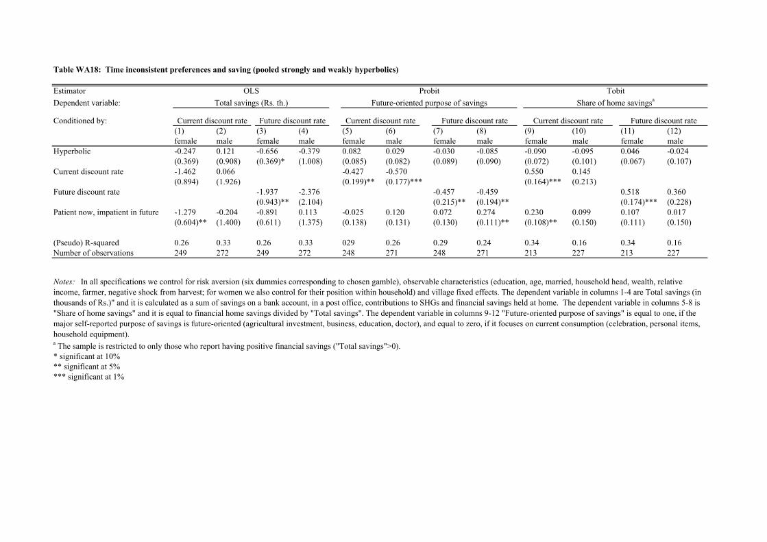
Table WA18: Time inconsistent preferences and saving (pooled strongly and weakly hyperbolics)
Estimator
Dependent variable:
Conditioned by:
(1) (2) (3) (4) (5) (6) (7) (8) (9) (10) (11) (12)
female male female male female male female male female male female male
Hyperbolic -0.247 0.121 -0.656 -0.379 0.082 0.029 -0.030 -0.085 -0.090 -0.095 0.046 -0.024
(0.369) (0.908) (0.369)* (1.008) (0.085) (0.082) (0.089) (0.090) (0.072) (0.101) (0.067) (0.107)
Current discount rate -1.462 0.066 -0.427 -0.570 0.550 0.145
(0.894) (1.926) (0.199)** (0.177)*** (0.164)*** (0.213)
Future discount rate -1.937 -2.376 -0.457 -0.459 0.518 0.360
(0.943)** (2.104) (0.215)** (0.194)** (0.174)*** (0.228)
Patient now, impatient in future -1.279 -0.204 -0.891 0.113 -0.025 0.120 0.072 0.274 0.230 0.099 0.107 0.017
(0.604)** (1.400) (0.611) (1.375) (0.138) (0.131) (0.130) (0.111)** (0.108)** (0.150) (0.111) (0.150)
(Pseudo) R-squared 0.26 0.33 0.26 0.33 029 0.26 0.29 0.24 0.34 0.16 0.34 0.16
Number of observations 249 272 249 272 248 271 248 271 213 227 213 227
a The sample is restricted to only those who report having positive financial savings ("Total savings">0).
* significant at 10%
** significant at 5%
*** significant at 1%
Future discount rate Current discount rate Future discount rate
Notes: In all specifications we control for risk aversion (six dummies corresponding to chosen gamble), observable characteristics (education, age, married, household head, wealth, relative
income, farmer, negative shock from harvest; for women we also control for their position within household) and village fixed effects. The dependent variable in columns 1-4 are Total savings (in
thousands of Rs.)" and it is calculated as a sum of savings on a bank account, in a post office, contributions to SHGs and financial savings held at home. The dependent variable in columns 5-8 is
"Share of home savings" and it is equal to financial home savings divided by "Total savings". The dependent variable in columns 9-12 "Future-oriented purpose of savings" is equal to one, if the
major self-reported purpose of savings is future-oriented (agricultural investment, business, education, doctor), and equal to zero, if it focuses on current consumption (celebration, personal items,
household equipment).
Current discount rate Future discount rate Current discount rate
Share of home savingsa
TobitOLS Probit
Total savings (Rs. th.) Future-oriented purpose of savings

Table WA19: Time inconsistent preferences and total savings without SHG savings
Estimator
Dependent variable:
Conditioned by:
(1) (2) (3) (4)
female male female male
Strongly hyperbolic -0.604 0.478 -0.955 -0.063
(0.440) (1.119) (0.432)** (1.184)
Weakly hyperbolic -0.148 -0.605 -0.253 -0.988
(0.523) (1.316) (0.524) (1.345)
Current discount rate -0.810 -0.263
(0.899) (2.032)
Future discount rate -1.372 -2.231
(0.932) (2.100)
Patient now, impatient in future -1.101 -0.237 -0.852 0.119
(0.592)* (1.396) (0.599) (1.371)
R-squared 0.25 0.32 0.25 0.32
Number of observations 249 272 249 272
* significant at 10%
** significant at 5%
*** significant at 1%
OLS
Total savings without SHG savings (Rs. th.)
Notes: In all specifications we control for risk aversion (six dummies corresponding to
chosen gamble), observable characteristics (education, age, married, household head, wealth,
relative income, farmer, negative shock from harvest; for women we also control for their
position within household) and village fixed effects. The dependent variable are Total
savings without SHG savings (in thousands of Rs.)" and it is calculated as a sum of savings
on a bank account, in a post office, and financial savings held at home.
Current discount rate Future discount rate
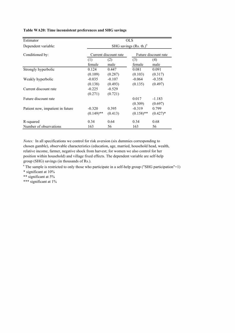
Table WA20: Time inconsistent preferences and SHG savings
Estimator
Dependent variable:
Conditioned by:
(1) (2) (3) (4)
female male female male
Strongly hyperbolic 0.124 0.447 0.081 0.091
(0.109) (0.287) (0.103) (0.317)
Weakly hyperbolic -0.035 -0.107 -0.064 -0.358
(0.138) (0.493) (0.135) (0.497)
Current discount rate -0.225 -0.529
(0.271) (0.721)
Future discount rate 0.017 -1.183
(0.309) (0.697)
Patient now, impatient in future -0.320 0.395 -0.319 0.799
(0.149)** (0.413) (0.158)** (0.427)*
R-squared 0.34 0.64 0.34 0.68
Number of observations 163 56 163 56
a The sample is restricted to only those who participate in a self-help group ("SHG participation"=1)
* significant at 10%
** significant at 5%
*** significant at 1%
OLS
SHG savings (Rs. th.)a
Notes: In all specifications we control for risk aversion (six dummies corresponding to
chosen gamble), observable characteristics (education, age, married, household head, wealth,
relative income, farmer, negative shock from harvest; for women we also control for her
position within household) and village fixed effects. The dependent variable are self-help
group (SHG) savings (in thousands of Rs.).
Current discount rate Future discount rate

Table WA21: Time inconsistent preferences and financial behavior (female, farmers excluded)
Estimator
Dependent variable:
Conditioned by:
Current
discount rate
Future
discount rate
Current
discount
rate
Future
discount
rate
Current
discount
rate
Future
discount
rate
Current
discount
rate
Future
discount
rate
(1) (2) (3) (4) (5) (6) (7) (8)
female female female female female female female female
Strongly hyperbolic -0.496 -0.863 -0.114 -0.055 0.399 0.182 0.229 0.219
(0.742) (0.685) (0.181) (0.123) (0.168)** (0.180) (0.078)** (0.133)*
Weakly hyperbolic 0.671 0.555 -0.051 -0.040 0.266 0.216 0.270 0.265
(1.140) (1.120) (0.115) (0.112) (0.177) (0.185) (0.103)*** (0.144)***
Current discount rate -1.132 0.232 -0.810 -0.122
(1.923) (0.282) (0.272)*** (0.435)
Future discount rate -1.513 0.143 -0.633 0.057
(2.012) (0.256) (0.360)* (0.452)
Patient now, impatient in future -1.344 -1.057 0.271 0.235 0.248 0.381 0.223 0.216
(0.609)** (0.743) (0.150)* (0.153) (0.192) (0.171)** (0.103) (0.131)
(Pseudo) R-squared 0.32 0.32 0.25 0.24 0.29 0.28 0.29 0.29
Observations 83 83 74 74 83 83 42 42
a The sample is restricted to only those who report having positive financial savings ("Total savings">0).
b The sample is restricted to only those who have any outstanding loan ("Loan"=1)
* significant at 10%
** significant at 5%
*** significant at 1%
Notes: Farmers are exluded from the sample. Standard errors corrected for clustering at the village level. In all specifications we control for risk
aversion (six dummies corresponding to chosen gamble), observable characteristics (education, age, married, household head, wealth, relative
income, farmer, negative shock from harvest; for women we also control for their position within household). The dependent variable in columns
1-2 are Total savings (in thousands of Rs.)" and it is calculated as a sum of savings on a bank account, in a post office, contributions to SHGs and
financial savings held at home. The dependent variable in columns 3-4 is "Share of home savings" and it is equal to financial home savings
divided by "Total savings". The dependent variable in columns 5-8 is "SHG borrowing" and it equals to one if an individual has an outstanding
loan from SHG. In columns 7-8 only those who borrow are included.
Probit Probit
SHG borrowing SHG borrowingb
OLS
Total savings (Rs. th.)
Tobit
Share of home savingsa

Table WA22: Determinants of time inconsistent preferences (farmers not controlled for)
Dependent variable Strongly hyperbolic Weakly hyperbolic
(1) (2) (3) (4) (5) (6)
female male female male female male
Gamble 2 0.075 0.334 -0.074 -0.034 -0.020 -0.034
(0.171) (0.155)** (0.068) (0.088) (0.085) (0.069)
Gamble 3 -0.015 0.261 -0.146 0.000 -0.013 0.025
(0.104) (0.168)* (0.076) (0.093) (0.083) (0.090)
Gamble 4 0.010 0.212 -0.097 0.086 0.040 -0.008
(0.116) (0.216) (0.055) (0.121) (0.108) (0.078)
Gamble 5 -0.035 0.280 -0.083 0.037 -0.016 0.077
(0.133) (0.189)* (0.068) (0.082) (0.079) (0.075)
Gamble 6 -0.062 0.256 -0.028 0.064 -0.100 0.043
(0.109) (0.180) (0.096) (0.123) (0.041) (0.108)
Education -0.002 0.002 0.000 0.006 0.003 -0.004
(0.011) (0.008) (0.005) (0.005) (0.009) (0.005)
Age -0.020 -0.001 0.016 0.006 -0.000 0.009
(0.012) (0.013) (0.018) (0.012) (0.012) (0.010)
(Age)2
0.000 0.000 -0.000 -0.000 -0.000 -0.000
(0.000) (0.000) (0.000) (0.000) (0.000) (0.000)
Married 0.134 -0.024 -0.126 -0.028 -0.113
(0.056)** (0.110) (0.111) (0.072) (0.097)
Household head 0.272 0.039 -0.056 -0.005 0.042
(0.163)* (0.084) (0.051) (0.094) (0.049)
Wealth 0.001 -0.009 -0.004 0.006 -0.029 -0.001
(0.017) (0.019) (0.012) (0.010) (0.009)*** (0.010)
Relative income 0.061 -0.046 -0.005 0.043 0.008 -0.050
(0.034)* (0.050) (0.052) (0.050) (0.045) (0.037)
Negative shock from harvest -0.033 -0.027 0.009 0.008 -0.040 -0.001
(0.059) (0.059) (0.052) (0.038) (0.028) (0.036)
Farmer
Pseudo R-squared 0.04 0.04 0.06 0.05 0.08 0.06
Observations 268 274 268 274 204 274
* significant at 10%
** significant at 5%
*** significant at 1%
Patient now, impatient in the
future
Note: In all columns we do not control for being a farmer. Standard errors corrected for clustering at the village level. Probit, marginal effects reported.
In column 1-2 the dependent variable "strongly hyperbolic preferences" equals to one if the respondent chose the more delayed reward two or more binary
choices later in the current time frame than in the future time frame. In columns 3-4 the dependent variable "weakly hyperbolic preferences" equals to one
if the respondent chose the more delayed reward one binary choice later in the current time frame than in the future time frame. In columns 5-6 the
dependent variable "Patient now, impatient in the future" equals to one if the respondent chose more delayed reward earlier in the current time frame than
in the future time frame.

Table WA23: Determinants of time inconsistent preferences (negative shock from harvest not controlled for)
Dependent variable Strongly hyperbolic Weakly hyperbolic
(1) (2) (3) (4) (5) (6)
female male female male female male
Gamble 2 0.067 0.360 -0.069 -0.037 -0.009 -0.034
(0.170) (0.158)** (0.069) (0.085) (0.089) (0.068)
Gamble 3 -0.038 0.269 -0.135 0.002 0.008 0.025
(0.108) (0.167)* (0.074) (0.093) (0.083) (0.091)
Gamble 4 -0.003 0.211 -0.090 0.091 0.067 -0.008
(0.124) (0.216) (0.057) (0.122) (0.113) (0.079)
Gamble 5 -0.038 0.285 -0.079 0.044 0.001 0.077
(0.136) (0.190)* (0.067) (0.082) (0.082) (0.076)
Gamble 6 -0.062 0.268 -0.023 0.054 -0.094 0.044
(0.111) (0.184) (0.094) (0.124) (0.042) (0.111)
Education -0.001 0.003 -0.000 0.004 0.002 -0.004
(0.010) (0.008) (0.005) (0.005) (0.009) (0.005)
Age -0.018 -0.002 0.017 0.007 0.001 0.009
(0.014) (0.014) (0.017) (0.012) (0.014) (0.010)
(Age)2 0.000 0.000 -0.000 -0.000 -0.000 -0.000
(0.000) (0.000) (0.000) (0.000) (0.000) (0.000)
Married 0.124 -0.028 -0.137 -0.031 -0.114
(0.056)* (0.119) (0.105)* (0.074) (0.097)
Household head 0.285 0.043 -0.068 -0.014 0.042
(0.155)** (0.080) (0.047) (0.091) (0.050)
Wealth -0.001 -0.012 -0.004 0.007 -0.028 -0.001
(0.017) (0.019) (0.011) (0.011) (0.009)*** (0.010)
Relative income 0.048 -0.037 -0.002 0.034 0.018 -0.050
(0.035) (0.052) (0.055) (0.048) (0.045) (0.037)
Negative shock from harvest
Farmer 0.057 0.032 -0.036 -0.040 -0.059 -0.000
(0.067) (0.052) (0.034) (0.035) (0.037) (0.043)
Pseudo R-squared 0.04 0.04 0.06 0.04 0.08 0.06
Observations 266 272 266 272 203 272
* significant at 10%
** significant at 5%
*** significant at 1%
Patient now, impatient in the
future
Note: In all columns we do not control for a negative shock from harvest. Standard errors corrected for clustering at the village level. Probit, marginal
effects reported. In column 1-2 the dependent variable "strongly hyperbolic preferences" equals to one if the respondent chose the more delayed
reward two or more binary choices later in the current time frame than in the future time frame. In columns 3-4 the dependent variable "weakly
hyperbolic preferences" equals to one if the respondent chose the more delayed reward one binary choice later in the current time frame than in the
future time frame. In columns 5-6 the dependent variable "Patient now, impatient in the future" equals to one if the respondent chose more delayed
reward earlier in the current time frame than in the future time frame.
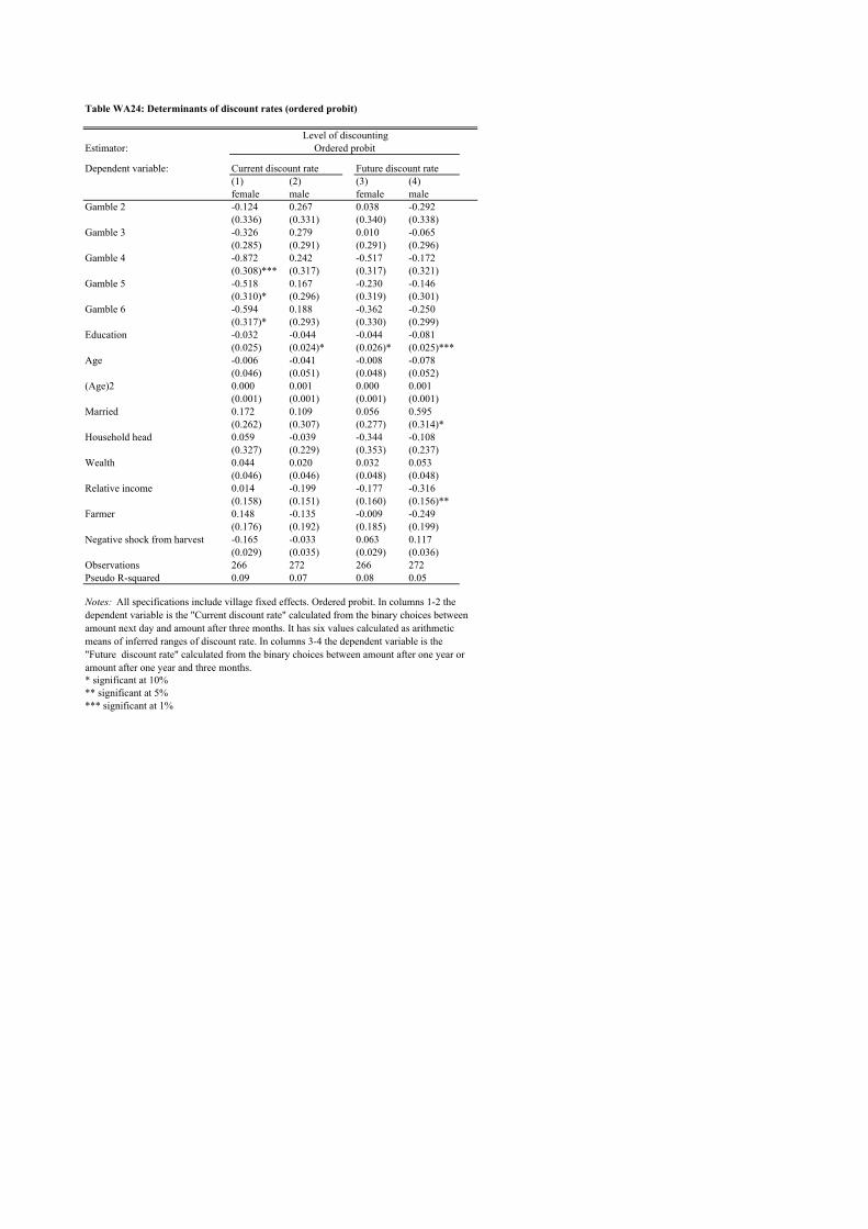
Table WA24: Determinants of discount rates (ordered probit)
Estimator:
Dependent variable: Current discount rate Future discount rate
(1) (2) (3) (4)
female male female male
Gamble 2 -0.124 0.267 0.038 -0.292
(0.336) (0.331) (0.340) (0.338)
Gamble 3 -0.326 0.279 0.010 -0.065
(0.285) (0.291) (0.291) (0.296)
Gamble 4 -0.872 0.242 -0.517 -0.172
(0.308)*** (0.317) (0.317) (0.321)
Gamble 5 -0.518 0.167 -0.230 -0.146
(0.310)* (0.296) (0.319) (0.301)
Gamble 6 -0.594 0.188 -0.362 -0.250
(0.317)* (0.293) (0.330) (0.299)
Education -0.032 -0.044 -0.044 -0.081
(0.025) (0.024)* (0.026)* (0.025)***
Age -0.006 -0.041 -0.008 -0.078
(0.046) (0.051) (0.048) (0.052)
(Age)2 0.000 0.001 0.000 0.001
(0.001) (0.001) (0.001) (0.001)
Married 0.172 0.109 0.056 0.595
(0.262) (0.307) (0.277) (0.314)*
Household head 0.059 -0.039 -0.344 -0.108
(0.327) (0.229) (0.353) (0.237)
Wealth 0.044 0.020 0.032 0.053
(0.046) (0.046) (0.048) (0.048)
Relative income 0.014 -0.199 -0.177 -0.316
(0.158) (0.151) (0.160) (0.156)**
Farmer 0.148 -0.135 -0.009 -0.249
(0.176) (0.192) (0.185) (0.199)
Negative shock from harvest -0.165 -0.033 0.063 0.117
(0.029) (0.035) (0.029) (0.036)
Observations 266 272 266 272
Pseudo R-squared 0.09 0.07 0.08 0.05
* significant at 10%
** significant at 5%
*** significant at 1%
Level of discounting
Notes: All specifications include village fixed effects. Ordered probit. In columns 1-2 the
dependent variable is the "Current discount rate" calculated from the binary choices between
amount next day and amount after three months. It has six values calculated as arithmetic
means of inferred ranges of discount rate. In columns 3-4 the dependent variable is the
"Future discount rate" calculated from the binary choices between amount after one year or
amount after one year and three months.
Ordered probit

Table WA25: Time inconsistent preferences and SHG borrowing (controlling for total savings)
Estimator
Dependent variable:
Conditioned by:
(1) (2) (3) (4) (5) (6) (7) (8) (9) (10) (11) (12)
female male female male female male female male female male female male
Strongly hyperbolic 0.267 0.069 0.036 0.058 0.403 0.052 0.237 0.024 0.317 -0.016 0.296 -0.070
(0.072)*** (0.080) (0.106) (0.082) (0.098)*** (0.050) (0.108)** (0.044) (0.076)*** (0.083) (0.085)** (0.077)
Weakly hyperbolic -0.043 -0.056 -0.123 -0.045 0.045 -0.061 -0.007 -0.062 0.050 -0.182 0.037 -0.184
(0.126) (0.068) (0.134) (0.073) (0.131) (0.022)* (0.129) (0.023)* (0.145) (0.046)*** (0.149) (0.046)***
Current discount rate -0.782 -0.112 -0.462 -0.083 -0.125 -0.243
(0.239)*** (0.122) (0.257)* (0.063) (0.343) (0.156)
Future discount rate -0.950 0.023 -0.669 -0.040 -0.131 -0.168
(0.251)*** (0.129) (0.277)** (0.068) (0.384) (0.163)
Patient now, impatient in future -0.015 -0.086 0.148 -0.074 0.102 -0.053 0.212 -0.045 0.241 -0.127 0.244 -0.100
(0.132) (0.066) (0.099) (0.070) (0.156) (0.024) (0.155) (0.030) (0.067)* (0.053) (0.065)* (0.074)
Total savings (Rs. th.) 0.067 0.004 0.062 0.004 0.027 -0.000 0.023 -0.000 0.045 0.015 0.045 0.013
(0.022)*** (0.005) (0.022)*** (0.005) (0.017) (0.002) (0.017) (0.002) (0.026)* (0.007)** (0.027) (0.007)**
Pseudo R-sqaured
Observations 239 261 239 261 232 250 232 250 139 140 139 140
a The sample is restricted to only those who have any outstanding loans ("Loan"=1)
* significant at 10%
** significant at 5%
*** significant at 1%
Current discount rate Future discount rate
Notes: In all specifications we control for total savings, risk aversion (six dummies corresponding to chosen gamble), observable characteristics (education, age, married, household head, wealth, relative income,
farmer, negative shock from harvest; for women we also control for their position within household) and village fixed effects. The dependent variable in columns 1-4 is "SHG participation" and it equals to one, if an
individual is a member of a self-help group (SHG). The dependent variable in columns 5-12 is "SHG borrowing" and it equals to one if if an individual has an outstanding loan from a self-help group (SHG). In
columns 9-12 only those who borrow are included.
Current discount rate Future discount rate Current discount rate Future discount rate
Probit Probit Probit
SHG participation SHG borrowing SHG borrowinga

Table WA26: Time inconsistent preferences and borrowing (controlling for total savings)
Estimator
Dependent variable:
Conditioned by:
(1) (2) (3) (4) (5) (6) (7) (8)
female male female male female male female male
Strongly hyperbolic 0.249 0.184 0.120 0.229 0.039 0.089 -0.121 0.111
(0.085)*** (0.091)* (0.100) (0.091)** (0.142) (0.117) (0.158) (0.125)
Weakly hyperbolic -0.022 0.102 -0.060 0.136 -0.062 0.140 -0.124 0.138
(0.121) (0.108) (0.124) (0.107) (0.193) (0.141) (0.196) (0.143)
Current discount rate -0.408 0.022 -0.503 0.115
(0.220)* (0.182) (0.342) (0.235)
Future discount rate -0.559 0.220 -0.523 0.073
(0.223)** (0.190) (0.415) (0.242)
Patient now, impatient in future -0.189 -0.023 -0.085 -0.057 0.228 0.090 0.253 0.062
(0.138) (0.127) (0.138) (0.127) (0.147) (0.168) (0.128) (0.177)
Total savings (Rs. th.) 0.013 -0.015 0.011 -0.015 -0.031 -0.001 -0.032
(0.016) (0.006)*** (0.016) (0.006)*** (0.021) (0.011) (0.021)
(Pseudo) R-squared
Observations 241 272 241 272 130 151 130 151
a The sample is restricted to only those who have any outstanding loans ("Loan"=1)
* significant at 10%
** significant at 5%
*** significant at 1%
Notes: In all specifications we control for total savings, risk aversion (six dummies corresponding to chosen gamble), observable characteristics
(education, age, married, household head, wealth, relative income, farmer, negative shock from harvest; for women we also control for their position
within household) and village fixed effects. The dependent variable in columns 1-4 is "Loan" and it equals to one, if an individual has an
outstanding loan from a bank, self-help group (SHG), NGO or moneylender. The dependent variable in columns 5-8 is "Delayed repayment of
outstanding loan" and it equals to one if the respondent reports being delayed on repayment of the outstanding loan for at least one installment.
Current discount rate Future discount rate Current discount rate Future discount rate
Probit Probit
Loan Delayed repayment of outstanding loana