How to establish life cycle inventories of agricultural ...formations.cirad.fr/analyse-cycle-de-vie/pdf/ThomasNemecek.pdf · How to establish life cycle inventories of agricultural

Federal Department of Economic Affairs FDEA

Agroscope Reckenholz-Tänikon Research Station ART

2 March 2010

How to establish life cycle inventories of agricultural products?

Thomas Nemecek

Agroscope Reckenholz-Tänikon Research Station ARTCH-8046 Zurich, Switzerlandhttp://[email protected]

How to establish life cycle inventories of agricultural products?T. Nemecek | © Agroscope Reckenholz-Tänikon Research Station ART 2

Overview

Defining system boundaries: temporal and process related How to get the LCI data: data survey vs. modelling ecoinvent database: Version 2.1 Future development to version 3.0 Direct field and farm emissions: how to estimate? Variability and uncertainty: Sources of variability Examples and implications Analysis of variability Assessment of uncertainty How to deal with missing data: generalisation and extrapolation Towards an integrated framework: SALCA Specific aspects of tropical crops Some recommendations


Defining system boundaries:Temporal system boundariesAnnual crops: Starting after harvest of previous crop (including fallow period

or catch crop, if no product) Ending with harvest of the considered crop

Permanent crops: Annual basis (1st January to 31st December) orMultiannual cropping cycle (distinguishing different phases:

planting, young plantation, main yielding phase, eradication)


Defining system boundaries:Example of crop production

Products:

Infrastructure:•Buildings•Machinery

Field work processes:•Soil cultivation•Fertilisation•Sowing•Chemical plant protection•Mechanical treatment•Harvest•Transport

Field production

Catch crops

Silage maizeSugar beetsFodder beetsBeetrootCarrotsCabbage

WheatBarleyRyeOatsGrain maizeCCMFaba beansSoya beansProtein peasSunflowersRape seed

Potatoes

Co-Product:Straw

Product treatment:

Grain drying

Potato grading

System boundaryR

esou

rces

Direct and indirect emissions

Manure storage

Animal excrements

Animal production system

Inputs:•Seed•Fertilisers (min. & org.)•Pesticides•Energy carriers•Irrigation water

© T. Nemecek, ART 2010


Defining system boundaries:Where to draw the line between animal and plant production?

Animal production (incl. feedstuffs, buildings, emissions, etc.)

Manure storageand treatment

Manure application(incl. machinery use and emissions)

Nutrient use in plant production

?

© Gaillard & Nemecek, 2006


Single crop or cropping system?

YearMonth 1 2 3 4 5 6 7 8 9 10 11 12 1 2 3 4 5 6 7 8 9 10 11 12 1 2 3 4 5 6 7 8 9 10 11 12

Year 4 5 6Month 1 2 3 4 5 6 7 8 9 10 11 12 1 2 3 4 5 6 7 8 9 10 11 12 1 2 3 4 5 6 7 8 9 10 11 12

Springbarley Grass-clover mixture ...

Fallo

w ..

.

... F

allo

w

1 2 3

... G

rass

-cl

over

mix

ture

PotatoesG

reen

man

ure

Winter wheat Forage catch crop Grain maize

© T. Nemecek, ART 2001


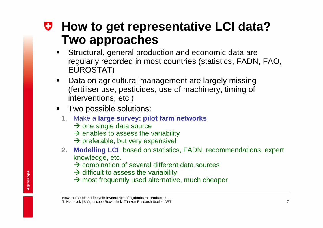
How to get representative LCI data?Two approaches Structural, general production and economic data are

regularly recorded in most countries (statistics, FADN, FAO, EUROSTAT)

Data on agricultural management are largely missing (fertiliser use, pesticides, use of machinery, timing of interventions, etc.)

Two possible solutions:1. Make a large survey: pilot farm networks one single data source enables to assess the variability preferable, but very expensive!

2. Modelling LCI: based on statistics, FADN, recommendations, expert knowledge, etc. combination of several different data sources difficult to assess the variability most frequently used alternative, much cheaper


Integrate environmental LCA into FADN Project supported by the Swiss Federal Office for Agriculture Time-frame: 2004 - 2010 with data acquisition from 2006 - 2008 Establish an operating system with 110 farms (during 3 years

with 60 in the first year) Establish an information technology infrastructure Training life cycle management principles in practiceDevelop concepts for evaluation and communication and

practice them with farmers and extension services Sectoral monitoring and environmental management of

farms

How to get representative LCI data? 1. Example of Swiss farm LCA networkProject Life Cycle Assessment – Farm Accountancy Data Network (LCA-FADN)


How to get representative LCI data? 1. Example of farm network / Project LCA-FADN: workflow

Existing FADN accountancy data

SynergiesFADN LCA-FADN

New FADNLife Cycle Assessment

Export ÖB-Stelle

Trus

t and

ac

coun

ting

offic

e

AccountancyData

FADN database

Accountancy-Software

(AGRO-TWIN)

Plausibility testsSALCAcheck

LCA validation and benchmarking

FAD

N

eval

uatio

n ce

ntre

Farm

LCA

cen

tre

Feedback to farmers

SALCAcalcLCA calculation

Technical data

SALCAprepdata extraction

Farm management software

(AGRO-TECH)

Accountancy data

Accountancy-Software

LCA data

© Agroscope ART 2010


How to get representative LCI data?2. Example of modelling LCI

Source: Nemecek, Erzinger (2004). Modelling representative life cycle inventories for Swiss arable crops. Int J LCA.

Information provided by seed suppliers and experts (survey)Chemical seed dressing

Pilot farm network (years 1994-96 from BLW et al. 1998)Pesticide applications

Pilot farm network (years 1994-96 from BLW et al. 1998) for farmyard manure

Types of fertilisers in organic systems

Import statistics (years 1996-98 from Rossier 2000) for mineral fertilisersPilot farm network (years 1994-96 from BLW et al. 1998) for farmyard manure

Types of fertilisers in integrated systems

Fertilising recommendations (Walther et al. 2001)Quantity of fertilisers

Work budget (planning tool, Näf 1996)Sowing and harvest dates

Gross-margin catalogue from the extension service (LBL et al. 2000)

Moisture contentQuantity of seedUse of machinery (number of passes)

Fertilising recommendations (Walther et al. 2001)Straw yields and crop residues

FADN ART (weighted means for 1996-2003)Yields for main products

Data source(s)Data category


Sources of LCI data:ecoinvent database v.2.1

More than 4000 generic LCI process datasets on energy supply, resource extraction, material supply, chemicals, metals, agriculture, waste management services, and transport services

Used by over 1200 members in more than 40 countries

Included in the leading LCA software and eco-design tools

Online access to LCI and LCIA results for all datasets

Based on industry data, compiled by independent experts

Consistent, validated and transparent

Continuously maintained

International in scope, including e.g. data on US agriculture, worldwide sourcing of raw materials and production of electronics in Asia

A joint initiative of the ETH domain and Swiss Federal Offices


Datasets for the biomassproduction in ecoinvent: Overview

1. Datasets on agricultural means of production: infrastructure (buildings and machinery) and its usage, fertilisers, pesticides, seed and animal feed

2. Datasets on agricultural and biomass products: • Arable crop products• Grass• Wood• Fibres

Swiss Centre For Life CycleInventories



Contents of ecoinvent Version 2.1What is covered in agriculture?

Production branches Buil

ding

s

Mac

hine

ry

Wor

k pr

oces

ses

Inpu

ts

Prod

ucts

CH

Pro

duct

s Eu

rope

Prod

ucts

Am

eric

a

Pro

duct

s As

ia

Arable cropsFodder cropsHorticulture (Field)Horticulture (Greenhouse)Fruit growingVineyardsCattle productionPig productionPoultry productionSheep production

relevant datasests availablepartly availablenot available



© ecoinvent centre, 2007


Contents of ecoinvent version 2.1Datasets for biomass production

Category Subcategory Number of datasetsagricultural means of production buildings 23agricultural means of production machinery 6agricultural means of production work processes 39agricultural means of production mineral fertiliser 24agricultural means of production organic fertiliser 5agricultural means of production pesticides 68agricultural means of production seed 26agricultural means of production feed 10agricultural production plant production 120agricultural production animal production 4biomass production 4wooden materials extraction 123wood energy fuels 13Total 465





Contents of ecoinvent version 2.1Crops and countries

CountriesBrazilCameroonChinaEuropeFranceGermanyGlobalIndiaMalaysiaPhilippinesScandinaviaSpainSwitzerlandThailandUSA

barley potatocotton protein peasfaba beans ramiefodder beets rape seedgrain maize ricegrass ryegrass silage silage maizegreen manure soy beanshay sugar beetshemp sugar canejute sunflowerkenaf sweet sorghumoil palm wheat

CerealsOil cropsProtein cropsFibre cropsGrass

Crops





ecoinvent database: online access


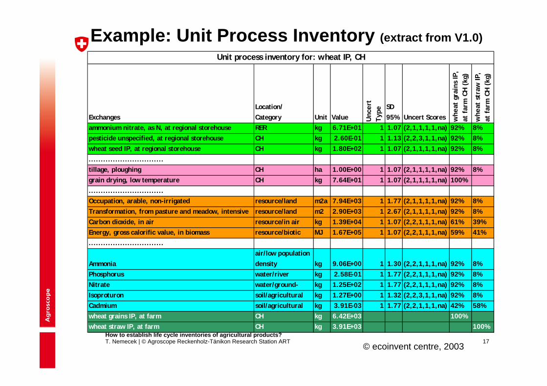
Example: Unit Process Inventory (extract from V1.0)

ExchangesLocation/Category Unit Value U

ncer

tTy

pe

SD95% Uncert Scores w

heat

gra

ins

IP,

at f

arm

CH

(kg

)

whe

at s

traw

IP,

at f

arm

CH

(kg

)

ammonium nitrate, as N, at regional storehouse RER kg 6.71E+01 1 1.07 (2,1,1,1,1,na) 92% 8%pesticide unspecified, at regional storehouse CH kg 2.60E-01 1 1.13 (2,2,3,1,1,na) 92% 8%wheat seed IP, at regional storehouse CH kg 1.80E+02 1 1.07 (2,1,1,1,1,na) 92% 8%...............................tillage, ploughing CH ha 1.00E+00 1 1.07 (2,1,1,1,1,na) 92% 8%grain drying, low temperature CH kg 7.64E+01 1 1.07 (2,1,1,1,1,na) 100%...............................Occupation, arable, non-irrigated resource/land m2a 7.94E+03 1 1.77 (2,1,1,1,1,na) 92% 8%Transformation, from pasture and meadow, intensive resource/land m2 2.90E+03 1 2.67 (2,1,1,1,1,na) 92% 8%Carbon dioxide, in air resource/in air kg 1.39E+04 1 1.07 (2,2,1,1,1,na) 61% 39%Energy, gross calorific value, in biomass resource/biotic MJ 1.67E+05 1 1.07 (2,2,1,1,1,na) 59% 41%...............................

Ammoniaair/low population density kg 9.06E+00 1 1.30 (2,2,1,1,1,na) 92% 8%

Phosphorus water/river kg 2.58E-01 1 1.77 (2,2,1,1,1,na) 92% 8%Nitrate water/ground- kg 1.25E+02 1 1.77 (2,2,1,1,1,na) 92% 8%Isoproturon soil/agricultural kg 1.27E+00 1 1.32 (2,2,3,1,1,na) 92% 8%Cadmium soil/agricultural kg 3.91E-03 1 1.77 (2,2,1,1,1,na) 42% 58%wheat grains IP, at farm CH kg 6.42E+03 100%wheat straw IP, at farm CH kg 3.91E+03 100%

Unit process inventory for: wheat IP, CH



Plans for the ecoinvent database v.3.0 – release 2011Co-operation with national database initiativesMore detail, more technologies, more completeness: International editorial board and broader supplier base Parameterisation (geography, time, technologies, markets) New data structure based on supply-use framework, allowing easier

production of national versions New indicators Sponsor-funded Open Access to individual datasetsMore frequent updating Improved uncertainty estimation and calculation facilities


New developments for ecoinvent V3.0:International editorial board and broader supplier base International editorial board Activity editors, for each industry activity and for household

activities Cross-cutting editors, to ensure consistency and monitor

developments across the entire database, both for specific (groups of) emissions, for geographical areas, scenarios, etc., and for the meta-data fields, e.g. uncertainty

Broader supplier base Making it easier for experts and lay users to contribute with new

data or corrections to existing data All such contributions will still be subject to our strict quality

control, review, and validation procedures before entering into the database


New developments for ecoinvent V3.0: ParameterisationGeographical parameters: Core international datasets + national differences Using GIS coordinates, all other area parameters can be

expressed: Country codes, areas with different population densities, habitat areas, watershed areas, etc. for site-dependent impact assessment

Temporal parameters (years) Scenario parameters (e.g. BaU, optimistic, pessimistic)Dataset-internal parameters Inheritance using parent child-relationships


New developments for ecoinvent V3.0: Better support for alternative modelling options

Attributional and consequential modelling: Average versus marginal market modelling Allocation versus substitution (system expansion) Several versions of attributional allocation

The unallocated (multi-functional) unit processes are the same for both models


Estimating direct field and farm emissionsUsually no measurement on site possibleTwo options: 1. Literature values, experiments: take a value for a given

situation Specific for the situation Difficult to find Not flexible Mitigation options usually cannot be considered 2. Modelling More flexible Mitigation options can be considered, depending on the model Level of detail should be consistent across the models No globally usable emission models available


Estimating direct field and farm emissions

Ideal emission models shouldReflect the underlying environmental mechanisms Be site and time dependentConsider the effect of soil and climateConsider the effect of management Be applicable under a wide range of different situations The different models should have a similar level of detail But also be usable: Parameters are measurable Data can be collected in a reasonable time Calculation is feasible

A compromise is needed!


SALCA emission modelsAmmonia (NH3)4 Emissions paths are modelled:1. Application of farm manure = f(fertiliser amount, NH3 and

NH4-concentration, covered area, saturation deficit in the air in function of average monthly temperature)

2. Application of mineral fertiliser = emission factors according to fertiliser type (2-15%, Asman 1992)

3. Emission from pasture = 5% of total N in excrements emitted as NH3

4. Emission from stable = emission factors dependent on animal category, housing system, farm manure type (liquid or solid) Source: Menzi et al. (1997)

© Agroscope ART, 2010


SALCA emission modelsNitrous oxide (N2O)

Fertilisers: Direct emissions: 1% of available N Symbiotic N-fixation in legumes: no emissionsCrop residues: emission factor 1% Storage of farmyard manure: emission factors 0.1% for liquid

manure and 2% for dung Pasture: emission factor 2% Induced Emissions: 1% of NH3-N and 0.75% of NO3-N

N2O in air: adapted method according to IPCC 2006, under consideration of induced N2O-Emissions:



SALCA emission modelsSALCA-nitrate

Input of mineral N through fertilisers (NH4, NO3, Amid-N)

N minerali-sation of soil organic matter

N uptakeplants

Leaching Leaching

Non leached N

+

GRUDAF:60 dt yield158 kg N uptake

Example:80 dt yield211 kg N uptake

Temperature dependent

N-Uptake functions(STICS)

Monthly N-uptake

Source: Richner et al. (2006)



SALCA emission modelsMethane (CH4) IPCC method 2 (Houghton et al. 1995) currently under revision Animal breading: Emissions from digestion = f(animal category, feeding) Emissions from storage of farm manure = f(animal category,

housing system)

Emission factors:Liquid manure: 10%Dung and pasture: 1%



SALCA emission modelsPhosphorus (P)4 kinds of P-emissions in water:

• Surface run-off in rivers (solved PO43-)

• Drainage losses in rivers (solved PO43-)

• Erosion in rivers (P bound to soil particles)• Leaching in ground water (solved PO4

3-)

Emissions are dependent of:• Soil characteristics (granulation, bulk density, soil water

balance) and drainage• Quantity of P-fertiliser• Type of P-fertiliser (manure, compost, mineral)• Field slope and distance to rivers• Quantity of eroded soil• Plant available P in upper soil

Source: Prasuhn (2006)© Agroscope ART, 2010


SALCA emission modelsHeavy metals

Input-Output-Balance (caused by farmer) per field for:Cd, Cu, Zn, Pb, Ni, Cr, Hg Inputs:

- Fertilisers (mineral and organic)- Seed- Pesticides- Feedstuff and auxiliary materials for animal breeding Outputs:

- Exported primary products (e.g. grains, meat)- Exported co-products (e.g. straw, animal manure)- Leaching to groundwater and drainage to surface water- Erosion to surface water Allocation for inputs caused by the farmer The final balance can be negative! Source: Freiermuth (2006)



Variability and uncertainty: Factors influencing environmental impacts

Crop management

Pedo-climatic conditions

Crop yield

Life cycle inventory

Environmental impacts

To understand the variability of

environmental impacts, we need to

look on the variability of the

influencing factors

Socio-economic conditions

© T. Nemecek ART, 2010


Global variability of yieldsExample: potato

medianq25%

q2.5%

Source: FAOSTAT

Cumulated potato world production as a function of the yield

05

101520253035404550

0.0 20.0 40.0 60.0 80.0 100.0

Cumulated world production [%]

Yiel

d [t/

ha]


T. Nemecek | © Agroscope Reckenholz-Tänikon Research Station ARTKey factors of crop LCI/LCA variability: example of wheat

Variability of environmental impacts:Wheat datasets in ecoinvent V2.01 (2007)

w heat grains, at farm

0.59

0.67

0.59

0.63

0.76

0.55

0.60

0.00 0.20 0.40 0.60 0.80

CH, IP

CH, ext

CH, org

Barrois, FR

Castilla, ES

Saxony, DE

US

GWP 100a, kg CO2-eq./kg

w heat grains, at farm

3.30

3.45

2.31

3.58

6.42

3.49

4.63

0.00 2.00 4.00 6.00 8.00

CH, IP

CH, ext

CH, org

Barrois, FR

Castilla, ES

Saxony, DE

US

energy demand, MJ-eq./kg

©ec

oinv

ent c

entre

200

7


Variability of environmental impacts: Energy demand per ha UAA (62 Swiss farms)

Energy demand per ha UAA

020000400006000080000

100000120000140000160000180000200000220000240000260000280000300000

31 22 21 22 23 11 21 21 15 11 11 14 11 22 21 11 11 21 21 51 13 21 53 51 51 21 21 51 55 51 51 11 11 21 14 21 22 16 53 52 53 21 53 21 55 23 21 21 11 51 53 53 56 51 11 53 53 53

MJ-

Eq.

Fa rmty pe D es c ription Fa rm ty pe D es c rip tio n1 1 a rab le fa rm ing 2 3 o th er cat tle1 3 ve ge ta b le cu ltivat io n 3 1 h orse s/g o ats/sh e ep1 4 f ruit cultivat io n 5 1 d airy fa rm / a ra ble fa rm in g com bin ed1 5 viticultu re 5 2 su ckler cow s / a rab le fa rm ing co m b ine d1 6 o th er cu ltu re s 5 3 p ig s a n d po u ltry / a ra ble fa rm in g com bine d2 1 d airy farm 5 5 d airy fa rm s / o th e r co m b in e d2 2 su ckler co ws 5 6 ca ttle / othe r co m b ine d



Variability of environmental impacts: Example: Energy demand per ha UAA (dairy farms)

Energy demand of dairy farms

0

10000

20000

30000

40000

50000

60000

70000

80000

1 2 3 4 5 6 7 8 9 10 11 12 13 14 15

MJ-

Eq./h

a U

AA

other inputs

emissions of animals

purchase of foodstuff

purchase of animals

PPP

fertiliser / nutrients

seeds

energy carriers

machines

buildings / equipment

Eutrophication of dairy farms

0

50

100

150

200

250

300

350

1 2 3 4 5 6 7 8 9 10 11 12 13 14 15

kg N

-Eq.

/ha

UA

Aother inputs

emissions of animals

purchase of foodstuff

purchase of animals

PPP

fertiliser / nutrients

seeds

energy carriers

machines

buildings / equipment



Variance control as a basis for environmentalmanagement

An balanced use of energy and fertilisers improves eco-efficiency. The best farms (1, 2) had the

lowest pesticide use per area unit.The orchards have high yields (high labour input) and a good physiological and ecological equilibrium.

(i)

y = 3.79x - 0.46r = 0.73, P = 0.007

0.0

2.0

4.0

6.0

0% 20% 40% 60% 80% 100% 120% 140% 160%

Farm No. 1

Farm No. 2

(iii)

y = 0.09x - 0.01r = 0.77, P = 0.003

0.00

0.05

0.10

0.15

0% 20% 40% 60% 80% 100% 120% 140% 160%

Coefficent of Variance

Farm No. 1

Farm No. 2

Energy use (MJ eq./$)

Aq. Eutrophication (PO4 eq./$)

M

M

Source: Mouron et al. (2006)


Variability and non-linearityAverages may lead to wrong results

Ammonia emission as a function of quantity of slurry applied. TAN = total ammonia N in the slurry (after Menzi et al. 1997)

0

2

4

6

8

10

12

14

16

0 10 20 30 40 50m3 of slurry

kg N

H3/

ha

0.0

0.1

0.2

0.3

0.4

0.5

0.6

0.7

0.8

kg N

H3-

N/k

g TA

N

NH3 emission (kg NH3/ha)

Relative emission rate (kg NH3-N/kg TAN)

1x40 m3 slurry 13.5 kg NH3

2x20 m3 slurry 17.4 kg NH3



Uncertainty assessment in ecoinvent V2.1: Pedigree matrix

Indicator score 1 2 3 4 5 Remarks

Reliability Verified data based on measurements

Verified data partly based on assumptions OR non-verified data based on measurements

Non-verified data partly based on qualified estimates

Qualified estimate (e.g. by industrial expert); data derived from theoretical information (stoichiometry, enthalpy, etc.)

Non-qualified estimate

verified means: published in public environmental reports of companies, official statistics, etcunverified means: personal information by letter, fax or e-mail

Completeness

Representative data from all sites relevant for the market considered over an adequate period to even out normal fluctuations

Representative data from >50% of the sites relevant for the market considered over an adequate period to even out normal fluctuations

Representative data from only some sites (<<50%) relevant for the market considered OR >50% of sites but from shorter periods

Representative data from only one site relevant for the market considered OR some sites but from shorter periods

Representativeness unknown or data from a small number of sites AND from shorter periods

Length of adequate period depends on process/technology

Temporal correlation

Less than 3 years of difference to our reference year (2000)




Age of data unknown or more than 15 years of difference to our reference year (2000)

less than 3 years means: data measured in 1997 or later;score for processes with investment cycles of <10 years;for other cases, scoring adjustments can be made accordingly

Geographical correlation

Data from area under study

Average data from larger area in which the area under study is included

Data from smaller area than area under study, or from similar area

Data from unknown OR distinctly different area (north america instead of middle east, OECD-Europe instead of Russia)

Similarity expressed in terms of enviornmental legislation. Suggestion for grouping:North America, Australia;European Union, Japan, South Africa; South America, North and Central Africa and Middle East;Russia, China, Far East Asia

Further technological correlation

Data from enterprises, processes and materials under study (i.e. identical technology)

Data on related processes or materials but same technology, OR Data from processes and materials under study but from different technology

Data on related processes or materials but different technology, OR data on laboratory scale processes and same technology

Data on related processes or materials but on laboratory scale of different technology

Examples for different technology:- steam turbine instead of motor propulsion in ships- emission factor B(a)P for diesel train based on lorry motor dataExamples for related processes or materials:- data for tyles instead of bricks production- data of refinery infrastructure for chemical

Sample size>100, continous measurement, balance of purchased products

>20 > 10, aggregated figure in env. report >=3 unknown sample size behind a figure reported in the

information source



Uncertainty assessment for French wheat

95% confidence interval



Potential use of multivariate statistics in LCA explain variability

Multivariate statistics (like principal component analysis, PCA) can be used to show similarities between environmental impacts It can be also used to group environmental profiles, e.g.

of cropsAnalysis based on a set of midpoint LCIA indicators In the study applied to crop inventories from SALCA

(Switzerland) and ecoinvent (global)


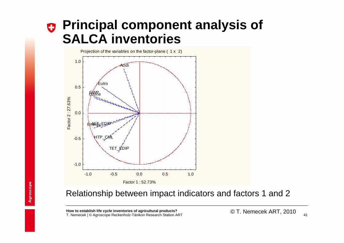
Principal component analysis of SALCA inventories

Eigenvalues of correlation matrixActive variables only

52.73%

27.63%

6.18% 5.07% 4.51% 2.24% .94% .70%

-1 0 1 2 3 4 5 6 7 8 9 10

Eigenvalue number

-0.5

0.0

0.5

1.0

1.5

2.0

2.5

3.0

3.5

4.0

4.5

5.0E

igen

valu

e

80% of variance explained by first two principal components© T. Nemecek ART, 2010



Relationship between impact indicators and factors 1 and 2

Projection of the variables on the factor-plane ( 1 x 2)

Energy

GWP Ozone

Eutro

Acidi

TET_EDIP

AET_EDIP

HTP_CML

-1.0 -0.5 0.0 0.5 1.0

Factor 1 : 52.73%

-1.0

-0.5

0.0

0.5

1.0

Fact

or 2

: 27

.63%



Factor 1: - can group crops- related to the yield

CER LEG MAI OIL ROOT VEG-6 -4 -2 0 2 4 6

Factor 1

-4

-3

-2

-1

0

1

2

3

4

5 Data for Swiss cropsfrom SALCA database: grouping by crop group(CER = cereals, LEG = legumes, MAI = maize, OIL = oil crops, ROOT = root crops, VEG = vegetables).

Fact

or2



Factor 2: - related to the farming system and theintensity

Conv Ipint Ipext Org-6 -4 -2 0 2 4 6

Factor 1

-4

-3

-2

-1

0

1

2

3

4

5

Data for Swiss crops from SALCA database: groupingby farming system(Conv=conventional, IPint = integrated intensive, IPext = integrated extensive, Org = organic). Fa

ctor

2




Yield is a key factor

Scatterplot (FALSR58_Res 14v*246c)

Factor 1 = -5.9426-2.1271*x

-3.0 -2.8 -2.6 -2.4 -2.2 -2.0 -1.8 -1.6 -1.4 -1.2 -1.0 -0.8 -0.6 -0.4

LnInvYield

-7

-6

-5

-4

-3

-2

-1

0

1

2Fa

ctor

1

LnInvYield:Factor 1: r2 = 0.4561



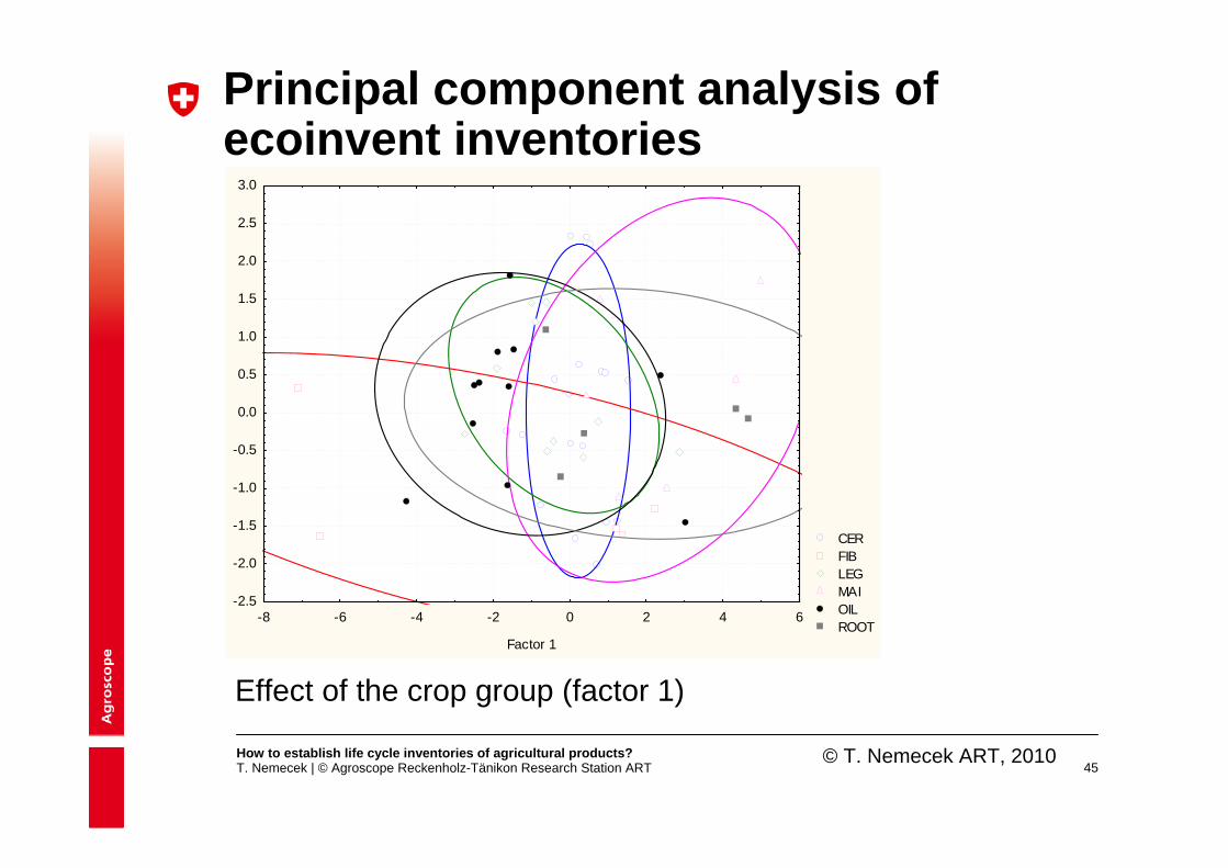
Principal component analysis of ecoinvent inventories

Effect of the crop group (factor 1)

CER FIB LEG MAI OIL ROOT

-8 -6 -4 -2 0 2 4 6

Factor 1

-2.5

-2.0

-1.5

-1.0

-0.5

0.0

0.5

1.0

1.5

2.0

2.5

3.0




Effect of the farming system (factor 2)

Conv IPint IPext Org

-8 -6 -4 -2 0 2 4 6

Factor 1

-2.5

-2.0

-1.5

-1.0

-0.5

0.0

0.5

1.0

1.5

2.0

2.5

3.0




Cereals in different countries

w heat barley rye

CH

FRES

DE

CH

CH

US

CH

FRES

DE

CH

CH

CH

RER

CH

CH

-8 -6 -4 -2 0 2 4 6

Factor 1

-2

-1

0

1

2

3



Potential use of multivariate statistics in LCA to explain variability

Between 76 and 80% of the variability could be explained by the first two principal components. Factor 1 crop (group) and yield Factor 2 farming system (conventional, integrated, extensive,

organic)More data are needed for more systematic analyses

The analysis helps to show similarities and differences between environmental profiles to find suitable proxies to derive simplified methods for extrapolations and approximations


How to fill data gaps in agricultural LCI?

The classical approach:1. Establish detailed and specific inventories for each

situationCurrently used alternatives:

2. Use proxies: what you think is the closest LCI (generalisation)

3. Streamlined LCA modelsNew approaches:

4. Extrapolation by yield correction5. Modular extrapolation method geographical extrapolation product extrapolation


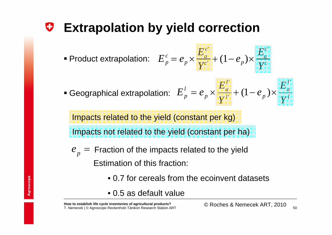
Extrapolation by yield correction

Product extrapolation:

Geographical extrapolation:

c

ca

pc

ca

pcp Y

EeYEeE

'

'

'

)1(

l

la

pl

la

plp Y

Ee

YE

eE'

'

'

)1(

Impacts related to the yield (constant per kg)

Impacts not related to the yield (constant per ha)

pe Fraction of the impacts related to the yieldEstimation of this fraction:

• 0.7 for cereals from the ecoinvent datasets

• 0.5 as default value© Roches & Nemecek ART, 2010


Modular EXtrapolation for Agricultural LCA (MEXALCA)

Basic idea: It is possible to split an inventory into different independent

modules. This enables easier adaptation of an existing inventory to a new

situation.

Working procedure:1. Establish a base inventory for one or several typical situations2. Split the inventory into independent modules3. Calculate unit inventories/impacts per module and input unit4. Determine amount of inputs used in each country (using global

estimators derived from FAOSTAT)5. Extrapolate inventory to any producing country6. Estimate global/regional impacts (medians, means, distribution)


Impacts for extrapolated situation

Input parameters:•yield per area unit•Mechanisation index•% of no-till area•kg N, P2O5, K2O applied•kg pesticide active ingredient•m3 water used•kg water evaporated

Good quality data availablefor some or all inputs

Global estimators(based on FAOSTAT)

Base crop inventory

Impacts per input unitBasic cropping operationsSoil tillageVariable machinery operationsN fertilisation, including N-emissionsP fertilisation, including P-emissionsK fertilisationPesticide applicationIrrigationProduct drying

Splitting

Calculation of unit impacts

Total impactsfor extrapolated

country y


country z


country x

0

0.05

0.1

0.15

0.2

0.25

0.3

0% 20% 40% 60% 80% 100%Percentage of the world potato production

GW

P 10

0 a

[kg

CO

2-eq

/kg]

Extrapolation

Extrapolation using MEXALCA

Global distribution of impacts



MEXALCA results: impacts per input unit

ModulesImpacts MachFix MachTill MachVar Nfert Pfert Kfert Pestic Irrigat Drying

non-renewable Energy [MJ-eq] 13604.50 1818.25 4621.45 70.91 31.26 10.69 341.5 9.988 0

GWP 100a [kg CO2-eq] 1074.68 118.49 272.66 13.45 2 0.614 15.127 0.247 0

photochemic O3 formation [kg ethylene-eq] 0.65 0.08 0.23 0.001 6E-04 2E-04 0.0092 2E-04 0

Nutrient enrichment [kg N-eq] 12.65 0.34 0.60 0.917 0.126 7E-04 0.023 2E-04 0

Acidification [kg SO2-eq] 9.38 0.95 1.80 0.282 0.039 0.003 0.099 9E-04 0

Aquatic ecotoxicity 100a [kg 1,4-DCB-eq] 56.92 0.13 0.45 0.015 0.404 0.007 114.99 4E-04 0

Terrestrial ecotoxicity 100a [kg 1,4-DCB-eq] 0.99 0.01 0.05 7E-04 0.009 3E-04 80.696 1E-04 0

Human toxicity 100a [kg 1,4-DCB-eq] 460.52 38.32 209.11 1.216 0.97 0.337 337.68 0.181 0

Potatoes

© Roches & Nemecek ART, 2010


MEXALCA results: impacts per kg of potato in the world

QUANTILES 2.5% 10.0% 25.0% median 75.0% 90.0% 97.5%Energy [MJ-eq] 9.11E-01 9.77E-01 1.27E+00 1.72E+00 3.00E+00 3.05E+00 4.15E+00GWP [kg CO2-eq] 7.38E-02 8.58E-02 1.11E-01 1.23E-01 1.91E-01 1.92E-01 2.05E-01O3 form. [kg ethylene-eq] 2.84E-05 3.13E-05 4.75E-05 6.59E-05 8.50E-05 8.53E-05 1.07E-04

IMPACTS Nutr. enrich. [kg N-eq] 1.85E-03 1.92E-03 2.41E-03 3.44E-03 5.54E-03 5.61E-03 7.52E-03Acidific. [kg SO2-eq] 9.44E-04 1.14E-03 1.23E-03 1.49E-03 2.27E-03 2.30E-03 2.82E-03Aquat. Ecotox.[kg 1,4-DCB-eq] 1.18E-02 1.65E-02 2.30E-02 3.06E-02 5.24E-02Terr. Ecotox. [kg 1,4-DCB-eq] 5.41E-03 9.15E-03 1.26E-02 1.89E-02 3.50E-02Human tox.[kg 1,4-DCB-eq] 6.91E-02 6.96E-02 7.26E-02 8.34E-02 1.01E-01 1.40E-01 2.00E-01

The modular inventory system enables us to calculate the inputs and impacts in any producing country and to calculate median and quantiles for the inputs and for the impacts for the global production (per kg of product or per cultivated ha).



Results: estimated distribution of GWP of the potato production

0

0.05

0.1

0.15

0.2

0.25

0.3

0% 20% 40% 60% 80% 100%Percentage of the world potato production

GW

P 1

00 a

[kg

CO

2-eq

/kg]



First validation: impacts per kg

2 4 6 8 10

24

68

10

Non renewable energy demand [MJ-eq]

ecoinvent

mod

ular

inve

ntor

y

y 1.163x -0.042r2 0.796

0.2 0.4 0.6 0.8 1.0 1.2

0.2

0.6

1.0

Global Warming Potential 100 years [kg CO2-eq]

ecoinvent

mod

ular

inve

ntor

y

Colours

barleywheatry epotatopea

y 0.386x 0.198r 2 0.493

r2 0.493

0.00005 0.00015 0.00025

0.00

005

0.00

020

Photochemical ozone formation [kg ethylene-eq]

mod

ular

inve

ntor

y

Colours

barleywheatry epot atopea

y 0.973x 0r2 0.939

0.01 0.02 0.03 0.04

0.01

0.02

0.03

0.04

Nutrient enrichment [kg N-eq]m

odul

ar in

vent

ory

Colours

barleywheatry epotatopea

y - 0.158x 0.021r 2 0.022

0.002 0.004 0.006 0.008 0.010

0.00

20.

006

0.01

0

Acidification [kg SO2-eq]

ecoinvent

mod

ular

inve

ntor

y

Colours

b arleywhea try ep otat op ea

y 1.103x 0.002r2 0.435



Sensitivity analysis Performed considering the median (=q50%), q10% and q90% of

each input (estimated variability of the inputs)

POT AT O INPUTSMachVar Nfert Pfert K fert Pestic Irrig at Drying

Quantiles q10% q90% q10% q90% q10% q90% q10% q90% q10% q90% q10% q90% q10% q90%IMPACTSnon-renewable energy [MJ-eq] -1% 7% -11% 22% -2% 3% -1% 4% -2% 7% -27% 62% 0% 0%GWP 100a [kg CO2-eq] -1% 5% -28% 55% -2% 2% -1% 3% -1% 4% -9% 21% 0% 0%photo. ozone formation [kg ethylene-Eq] -1% 11% -5% 11% -1% 1% -1% 3% -2% 6% -15% 34% 0% 0%nutrient enrichm ent [kg N -eq] 0% 0% -64% 125% -4% 5% 0% 0% 0% 0% 0% 1% 0% 0%Acidif icat ion [kg SO2-Eq] 0% 3% -47% 93% -3% 3% 0% 1% -1% 2% -3% 6% 0% 0%Aquatic ecotoxic ity, 100a [kg 1,4-DCB-Eq] 0% 0% 0% 1% -3% 4% 0% 0% -76% 288% 0% 0% 0% 0%Terres trial ecotoxic ity, 100a [kg 1,4-DCB-Eq] 0% 0% 0% 0% 0% 0% 0% 0% -99% 377% 0% 0% 0% 0%Human toxicity, 100a [kg 1,4-DC B-Eq] -1% 7% -4% 8% -1% 2% -1% 3% -43% 165% -11% 25% 0% 0%

Variation: 5 to 10% Variation: 10 to 50% Variation: 50 to 100% Variation: > 100%



Potentials of extrapolation

Extrapolation cannot replace data collection and the establishment of detailed and specific inventories Very important time saving possible Allows to create generic data sets on global and multinational level Assessment of global variability Fairly good estimates possible for energy demand, global warming and

ozone formation, land occupationDifficult for eutrophication and acidification (no site-specific parameters

considered) and toxicity (no detailed information on pesticide active ingredients)Can be used as first approximation and where ingredients is not so

relevant


SALCA: An integrated concept for agricultural environmental assessment

SALCA = Swiss Agricultural Life Cycle Assessment

SALCA consists of the following elements:Database for life cycle inventories for agriculture (in collaboration

with ecoinvent)Models for the calculation of direct emissions from field and farm A selection of impact assessment methods (midpoints)Methods for the assessment of impacts on biodiversity and soil

qualityCalculation tools for agricultural systems (farm, crop) Interpretation scheme for agricultural LCACommunication concept for the environmental management of

farms


SALCA calculation tools

Large variability large number of calculations automation requiredGeneric parametrised system modelling for farms and crops: SALCA-farm: generic LCA system for farms SALCA-crop: generic LCA system for arable crops and forage

production systems The templates are designed in order to cover all farms/crops All elements, which occur in at least one system must be

included Variables are defined, which can describe the different

quantities of inputs The variables that are not relevant for a particular system are

set to zeroModular structure


Data entry

Produktionsinventar.xls

Production inventory:C

omm

on dataentry

of all param

etersforall

tools

Input dataSA

LCA

heavy

metals

Input dataS

ALC

A

(TEA

M/S

imaP

ro)

Input dataS

ALC

A-soilquality

Input dataS

ALC

A-erosion

Input dataS

ALC

A-nitrate

Internal Links in EXCEL-sheet

SALC

A-H

eavym

etalsC

alculations

SALC

A

(TEAM

/SimaPro)

LCI C

alculations

SALC

A-soil

qualityC

alculations

SALC

A-biodiversity

Data entry

Calculations

(separate tool)

SALC

A-N

itrateC

alculations 6 separate tools in EXCEL: dataentry can be donethrough thecommonproduction inventory ordirectly in the tool

LIFE CYCLE INVENTORY (LCI)

LIFE CYCLE IMPACT ASSESSMENT (LCIA)

Transfer LCI data

SALC

A

(TEAM

/SimaPro)

LCIA

Calculation

Modular architecture of the tool SALCA-crop V3.1

© R. Freiermuth, T. Nemecek, ART 2010

SALC

A-Erosion

Calculations

Data transfer by macrosInput dataS

ALC

A-field

SALC

A-Field

(otherdirectem

issions)C

alculations


Specific aspects of tropical production systems: relevant LCI aspects Less managed production higher variability more dependent on the environment Labour input instead of machinery how to consider manpower?Use of draught animals how to consider?Reconsider the delimitation between plant and animal

production Adaptation of emission models to the conditions of the tropics

and subtropics (soil, climate)


Recommendations for agricultural LCILarge variability many observations neededCollect detailed farm management dataStandardised methodologyAutomated calculationUse of standard LCI formats (EcoSpold, ILCD)Need for a standardised format for agricultural

management dataRegionalisation, use of GISVariability and uncertainty should be assessed as

standard Infrastructure should be includedDevelopment of globally applicable emission models


Thanks toThanks toThanks to

My colleagues: GMy colleagues: GMy colleagues: Gééérard Gaillard, Ruth Freiermuth, rard Gaillard, Ruth Freiermuth, rard Gaillard, Ruth Freiermuth, Martina Martina Martina AligAligAlig, Daniel, Baumgartner, Anne , Daniel, Baumgartner, Anne , Daniel, Baumgartner, Anne RochesRochesRoches, , , Katharina Katharina Katharina PlassmannPlassmannPlassmannEcoinvent centreEcoinvent centreEcoinvent centreUnilever: Unilever: Unilever: LlorenLlorenLlorenççç MilMilMilààà i Canals, Sarah i Canals, Sarah i Canals, Sarah SimSimSim, , , TirmaTirmaTirma

GarciaGarciaGarcia---SuarezSuarezSuarez

You for your kind attention!You for your kind attention!You for your kind attention!

Documents

How to establish life cycle inventories of agricultural ...formations.cirad.fr/analyse-cycle-de-vie/pdf/ThomasNemecek.pdf · How to establish life cycle inventories of agricultural