Inventories and the business cycle: An equilibrium

analysis of (S,s) policies

Aubhik Khan1

Federal Reserve Bank of Philadelphia

Julia K. Thomas

University of Minnesota

Federal Reserve Bank of Minneapolis

October 2002 preliminary draft

1This paper has been presented at the 2002 Midwest Macroeconomics and Society for

Economic Dynamics meetings. We thank session participants and, in particular, Tony Smith

and Randall Wright, for their comments. The views expressed in this paper do not necessarily

reflect those of the Federal Reserve Banks of Minneapolis or Philadelphia.

1 Introduction

Inventory investment is both procyclical and volatile. Changes in firms’ inven-

tory holdings appear to account for almost half of the decline in production during

recessions.1 Moreover, the comovement between inventory investment and final sales

raises the variance of production beyond that of sales. Historically, such observations

have often prompted researchers to emphasize inventory investment as central to an

understanding of aggregate fluctuations.2 Blinder (1990), for example, concludes that

“business cycles are, to a surprisingly large degree, inventory cycles”.3 By contrast,

modern business cycle theory has been surprisingly silent on the topic of inventories.4

We study a dynamic stochastic general equilibrium model where, given nonconvex

factor adjustment costs, producers follow generalized (S, s) inventory policies with

regard to intermediate inputs. In particular, we extend the basic equilibrium business

cycle model to include fixed costs associated with the acquisition of intermediate

inputs for use in final goods production. Given these costs, final goods firms (a)

maintain inventories of intermediate inputs, and (b) adjust these inventories only

when their stock is sufficiently far from a target level. Our equilibrium analysis

implies that this target level varies endogenously with the aggregate state of the

economy. Because adjustment costs differ across firms, in addition to productivity

and capital, the aggregate state vector includes a distribution of these producers over

inventory levels.5

Our objective is two-fold. First, we evaluate the ability of our equilibrium general-

1Ramey and West (1999) show that, on average, the change in real inventory investment, relative

to the change in real gross domestic production, accounts for 49 percent of the decline in output

experienced during postwar U.S. recessions.2See Blinder and Maccini (1991).3Blinder (1990) page viii.4When inventories are included in equilibrium models, their role is generally inconsistent with their

definition. See, for example, Kydland and Prescott (1982) and Christiano (1988), where inventories

are factors of production, or Kahn, McConnell and Perez-Quiros (2001), where they are a source of

household utility.5At times, some producers completely exhaust their input stocks. In such instances, the non-

negativity constraint on inventories binds, which necessitates a nonlinear solution of the model.

1

ized (S, s) inventory model to reproduce salient empirical regularities. In particular,

we focus on the cyclicality and variability of inventories, and the relative volatility

of production and sales, as described below. Second, we examine the model’s pre-

dictions for the role of inventories in aggregate fluctuations. This provides a formal

analysis of the extent to which the existence of inventory adjustment amplifies or

prolongs cyclical movements in production.

To assess the usefulness of our model in identifying the role of inventories in the

business cycle, we evaluate its ability to reproduce (1) the volatility of inventory in-

vestment relative to production, (2) the procyclicality of inventory investment and

(3) the greater volatility of production over that of sales. We view these three empir-

ical regularities as essential characteristics of any formal analysis of the cyclical role

of inventories. When we calibrate our equilibrium business cycle model of inventories

to reproduce the average inventory-to-sales ratio in the postwar U.S. data, we find

that it is able to explain half of the measured cyclical variability of inventory in-

vestment. Furthermore, inventory investment is procyclical, and production is more

volatile than sales, as consistent with the data.

Examining our model’s predictions for the aggregate dynamics of output, con-

sumption, investment and employment, we find that the business cycle with inven-

tories is broadly similar to that generated by a comparable model without them.

Nonetheless, the inventory model yields somewhat higher variability in employment,

and lower variability in consumption and investment. Thus our equilibrium analy-

sis, which necessarily endogenizes final sales, alters our understanding of the role of

inventory accumulation for cyclical movements in GDP. In particular, we find that

the positive correlation between final sales and net inventory investment does not

imply that inventories necessarily amplify aggregate fluctuations in production. The

dynamics of final sales are altered by their presence. In the context of our equilibrium

business cycle model, the introduction of inventories does not substantially raise the

variability of production, because it lowers the variability of final sales.

2

2 A brief survey of empirical regularities

In this section, we discuss the small set of empirical regularities concerning in-

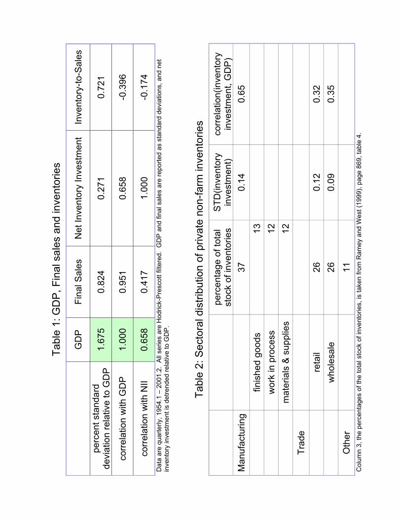
ventory investment that are most relevant to our analysis.6 Table 1 summarizes the

business cycle behavior of GDP, final sales, changes in private nonfarm inventories

and the inventory-to-sales ratio in postwar U.S. data.7 Note first that the relative

variability of inventory investment is large. In particular, though inventory invest-

ment’s share of gross domestic production averages less than one-half of one percent,

its standard deviation is 27 percent that of output. Next, net inventory investment

is procyclical; its correlation coefficient with GDP is 0.66. Moreover, as the correla-

tion between inventory investment and final sales is itself positive, 0.42 for the data

summarized in table 1, the standard deviation of production substantially exceeds

that of sales. It is this second positive correlation that is commonly interpreted as

evidence that fluctuations in inventory investment increase the variability of GDP.

Thus Ramey and West (1999, page 874) suggest that inventories “seem to amplify,

rather than mute movements in production”.

Our interest is in examining this thesis using dynamic stochastic general equilib-

rium analysis. However, inventories have received relatively little emphasis in general

equilibrium models of aggregate fluctuations. Given positive real interest rates, the

first challenge in any formal analysis of inventory adjustment is to explain why they

exist. By far the most common approach is to assume that production is costly

to adjust, and that the associated costs are continuous functions of the change in

production. This is the production smoothing model which, in its simplest form, as-

sumes that final sales are an exogenous stochastic series, and that adjustments to the

level of production incur convex costs. As a result, firms use inventories to smooth

6More extensive surveys are available in Fitzgerald (1997), Horstein (1998) and Ramey and West

(1999).7The table is based on U.S. quarterly data, 1953:1 - 2002:2, seasonally adjusted and chained in

1996 dollars. GDP and final sales are reported as percentage standard deviations, detrended using a

Hodrick-Prescott filter with a weight of 1600. Net investment in private nonfarm inventories xt, is

detrended relative to GDP, yt. The detrended series is xt−xtyt

, where xt is the HP-trend of the series

and yt is the trend for GDP.

3

production in the face of fluctuations in sales. An apparent limitation of the model

is it applies to a narrow subset of inventories, finished manufacturing goods.8 As il-

lustrated in Table 2, these are only 13 percent of the total. The remaining stocks are

commonly rationalized as the result of nonconvex order or delivery costs (see Blinder

and Maccini (1991)).9 Such costs lead firms to adopt (S,s) inventory adjustment poli-

cies, ordering only when their stocks are sufficiently far from a target level. It is the

prominence of inventories associated with nonconvex adjustment costs that leads to

us to the first defining feature of our analysis; we model (S,s) inventory management.

In table 2, we also see that inventories of intermediate inputs are twice the size

of finished goods in manufacturing. Furthermore, manufacturing inventories are far

more cyclical than retail and wholesale inventories, the other main components of

private nonfarm inventories. Humphreys, Maccini and Schuh (2001) undertake a vari-

ance decomposition and find that these input inventories are three times as volatile

as finished goods within manufacturing. Taken together, these findings motivate the

second defining feature of our analysis; we model inventories as stocks of intermediate

goods.10

3 Model

There are three types of optimizing agents in the economy, households, interme-

diate goods producers and final goods firms. Households supply labor to both types

of producers and purchase consumption from final goods firms. They save using asset

8Another difficulty, discussed at length by Blinder and Maccini (1991), is that the basic model,

driven by exogenous fluctuations in sales, predicts that production is less variable than sales, and that

sales and inventory investment are negatively correlated. Ramey (1991) shows that these inconsisten-

cies with the data may be resolved if there are increasing returns to production, while Eichenbaum

(1991) explores productivity shocks and Coen-Pirani (2002) integrates the stockout avoidance motive

of Kahn (1987) in a model of industry equilibrium.9An excellent example is Hall and Rust (1999), who show that a generalised (S, s) decision rule

explains the actual inventory investment behaviour of a U.S. steel wholesaler.10An equilibrium analysis of retail finished goods inventories is undertaken by Fisher and Hornstein

(2000), who use an (S, s) model to explain the higher volatility of production relative to sales.

4

markets where they trade shares that entitle them to the earnings of both interme-

diate and final goods producers. All firms in the economy are perfectly competitive.

First, identical intermediate goods producers own capital and hire labor for produc-

tion. They sell their output to, and purchase investment goods from, final goods

producers. Next, final goods firms use intermediate inputs and labor to produce

output that may be used for consumption or capital accumulation.

We provide an explicit role for inventories by assuming that final goods firms face

fixed costs of ordering or accepting deliveries of intermediate inputs. In particular,

as the costs are independent of order size, these firms choose to hold stocks of inputs,

s, where s ∈ S ⊆ R+. Further, the costs vary across final goods firms, so some

will adjust their inventory holdings, while others will not, at any point in time. As a

result, the model yields an endogenous distribution of final goods firms over inventory

levels, µ : B(S) → [0, 1], where µ(s) represents the measure of firms with start-of-

period inventories s.

The economy’s aggregate state is (z,Ξ), where Ξ ≡ (K,µ) represents the en-

dogenous state vector. K is the aggregate capital stock held by intermediate goods

firms, and z is total factor productivity in the production of intermediate inputs.

The distribution of firms over inventory levels evolves according to a mapping Γµ,

µ0 = Γµ (z,Ξ), and capital similarly evolves according to K 0 = ΓK (z,Ξ).11 For con-

venience, we assume that productivity follows a Markov Chain, z ∈ {z1, . . . , zNz},where

Pr¡z0 = zj | z = zi

¢ ≡ πij ≥ 0, (1)

andPNz

j=1 πij = 1 for each i = 1, . . . , Nz. Except where necessary for clarity, we

suppress the index for current productivity below.

All producers employ labour at the real wage, ω (z,Ξ), and those involved in the

production of final goods purchase intermediate inputs at the relative price q (z,Ξ).

Finally, all firms, whether producing intermediate inputs or final goods, value current

11Throughout the paper, primes indicate one-period ahead values. We define Γµ in section 3.2.3,

following the description of firms’ problems, and ΓK in section 3.4.

5

profits by the final output price p(z,Ξ) and discount future earnings by β.12 For

brevity, we suppress the arguments of ω, q and p where possible below.

3.1 Intermediate goods producers

The representative intermediate goods firm produces using capital, k, and labor,

l, through a constant returns to scale technology, zF (k, l). Intermediate inputs are

sold to final goods firms at the relative price q. The producer may adjust next

period’s capital stock using final goods as investment. Capital depreciates at the rate

δ ∈ (0, 1). Equation 2 below is the functional equation describing the intermediategoods firm’s problem. The value function W is a function of the aggregate state

(z,Ξ), which determines the prices (p, q and ω). Ξ evolves over time according to

µ0 = Γµ(z,Ξ) and K 0 = ΓK(z,Ξ) where Ξ ≡ (K,µ), and changes in productivity

follow the law of motion described in (1).

W (k; z,Ξ) = maxk0,l

µphqzF (k, l) + (1− δ) k − k0 − ωl

i+ β

NzXj=1

πijW¡k0; zj ,Ξ0

¢¶(2)

The following efficiency conditions describe the producer’s selection of employment

and investment.

zD2F (k, l) =ω

q(3)

βNzXj=1

πijD1W¡k0; zj ,Ξ0

¢= p (4)

Because F is linearly homogenous, the firm’s decision rules for employment and

production are proportional to its capital stock; l (k) ≡ L(z,Ξ)k where L (z,Ξ) solves

(3) as a function of (z, ω (z,Ξ) , q (z,Ξ)), and production is given by x(k; z,Ξ) =

zF (1, L(z,Ξ))k. This means that current profits are linear in k; π(z,Ξ) ≡ qzF (1, L(z,Ξ))+

(1 − δ) − ωL(z,Ξ). It is straightforward to show that this property is inherited by

12This is equivalent to requiring that firms discount by 1 + rt,t+k =pt

βkpt+kbetween dates t and

t + k, where p represents households’ current valuation of output and β their subjective discount

factor. This discounting rule is an implication of equilibrium, as discussed in section 3.4.

6

the value function; W (k; z,Ξ) = w (z; ξ) k, where

w (z,Ξ) · k = maxk0

p(z,Ξ)hπ(z,Ξ)k − k0

i+ β

NzXj=1

πijw¡zj ,Ξ

0¢ k0.Equation 4 then implies that an interior choice of investment places the following

restriction on the equilibrium price of final output.

p(z,Ξ) = βNzXj=1

πijw¡zj ,Ξ

0¢ . (5)

When (5) is satisfied, the intermediate goods firm is indifferent to any level of k0 and

will purchase investment as the residual from final goods production after consump-

tion.

3.2 Final goods producers

There are a large number of final goods firms, each facing time-varying costs

of arranging deliveries or sales of intermediate inputs. Given differences in delivery

costs, some firms adjust their stocks, while others do not, at any date. Thus, firms

are distinguished by their inventories of intermediate goods.

At the start of any date, a final goods firm is identified by its inventory holdings,

s, and its current delivery cost, ξ ∈ [A, B]. This cost is denominated in hours

of labor and drawn from a time-invariant distribution H (ξ) common across firms.

Intermediate inputs used in the current period, m, and labor, n, are the sole factors

of final goods production, y = G (m,n), where G exhibits decreasing returns to scale.

Note that technology is common across these firms; the only source of heterogeneity

in production arises from differences in inventories.

The timing of final goods firms’ decisions is as follows. At the beginning of each

period, any such firm observes the aggregate state (z,Ξ) as well as its current deliv-

ery cost ξ. Before production, it undertakes an inventory adjustment decision. In

particular, the firm may absorb its fixed cost and adjust its stock of intermediate

inputs available for production, s1 ≥ 0. Letting xm denote the chosen size of such

7

an adjustment, the stock of intermediate inputs available for current production be-

comes s1 = s + xm. Alternatively, the firm can avoid the cost, set xm = 0, and

enter production with its initial stock; s1 = s. Following the inventory adjustment

decision, the firm determines current production, selecting m ∈ [0, s1] and n ∈ R+.

Intermediate inputs fully depreciate in use, and the remaining stock with which the

firm begins next period is denoted s0. Measuring adjustment costs in units of final

output using the wage rate, ω, the firm’s order choice is summarized below.

order size total order costs production-time stock next-period stock

xm 6= 0 ωξ + qxm s1 = s+ xm s0 = s1 −m

xm = 0 0 s1 = s s0 = s−m

We assume that there is a storage cost associated with holding inputs unused through-

out the period. This cost is proportional to the level of inventories held; in particular,

given end of period inventories s0, the firm’s total cost of storage is σs0 where σ > 0.

Let E (s, ξ; z,Ξ) represent the expected discounted value of a final goods firm with

start-of-date inventory holdings s and fixed order cost ξ. We describe the problem

facing such a firm using (6) - (9) below. First, for convenience, we define the beginning

of period expected value of the firm, prior to the realization of its fixed cost, but given

(s; z,Ξ).

V (s; z,Ξ) ≡Z B

AE (s, ξ; z,Ξ)H (dξ) (6)

Next, we divide the period into two subperiods, adjustment-time and production-

time, and we break the description of the firm’s problem into the distinct problems

it faces as it enters into each of these subperiods.

3.2.1 Production decisions

Beginning with the second subperiod, let E1(s1; z,Ξ) represent the value of en-

tering production with inventories s1. Given this stock of intermediate input available

for production, the firm selects its current employment, n, and inventories for next

8

period, s0, (hence current input usage, m = s1 − s0) to solve

E1 (s1; z,Ξ) = maxs0≥0,n

³phG¡s1 − s0, n

¢− ωn− σs0i+ β

NzXj=1

πijV¡s0; zj ,Ξ0

¢´, (7)

taking prices (p, ω and q), and the evolution of Ξ0 ≡ (K 0, µ0) according to ΓK and

Γµ, as given. Given the production-time stock of intermediate inputs, s1, and the

continuation value of inventories of these inputs, V (s0; zj ,Ξ0), equation (7) yields both

the firm’s employment (in production) decision, which satisfies D2G (s1 − s0, n) = ω,

and its use of intermediate inputs. Let N (s1; z,Ξ) describe its employment and

S(s1; z,Ξ) its stock of intermediate input retained for future use. Current production

of final goods is Y (s1; z,Ξ) = G (s1 − S(s1; z,Ξ), N(s1; z,Ξ)). Thus, we have decision

rules for employment, production, and next-period inventories as functions of the

production-time stock s1.

3.2.2 Inventory adjustment decisions

Given the middle-of-period valuation of the firm, E1, we now examine the in-

ventory adjustment decision that precedes production. At the start of the period,

for a final goods firm with beginning of period inventories s and adjustment cost ξ,

equations (8) - (9) describes the (s, ξ) firm’s determination of (i) whether to place an

order and (ii) the target inventory level with which to begin the production subpe-

riod, conditional on an order. The first term in the braces of (8) represents the net

value of stock adjustment, (the gross adjustment value less the value of the payments

associated with the fixed delivery cost,) while the second term represents the value

of entering production with the beginning of period input stock.

E (s, ξ; z,Ξ) = pqs+maxn−pωξ +EA(z,Ξ),−pqs+E1 (s; z,Ξ)

o(8)

EA(z,Ξ) ≡ maxs1≥0

³−pqs1 +E1 (s1; z,Ξ)

´(9)

Note that the target inventory choice in (9) is independent of both the current

inventory level, s, and fixed cost, ξ. Thus, all firms that adjust their inventory

9

holdings choose the same production-time level, and achieve the same gross value of

adjustment, EA(z,Ξ). Let s∗ ≡ s∗(z,Ξ) denote this common target, which solves

(9) as a function of the aggregate state of the economy. Equation (7) then implies

common employment and intermediate input use choices across all adjusting firms,

as well as identical inventory holdings among these firms at the beginning of the next

period.

Turning to the decision of whether to adjust to the target level of inventories, it

is immediate from equation (8) that a firm will place an order if its fixed cost falls

at or below eξ(s; z,Ξ), the cost that equates the net value of inventory adjustment tothe value of non-adjustment.

−pωeξ(s; z,Ξ) +EA(z,Ξ) = E1 (s; z,Ξ)− pqs (10)

Given the support of the cost distribution, and using (10) above, we define ξ(s; z,Ξ)

as the type-specific threshold costs separating those firms that place orders from those

that do not.

ξ(s; z,Ξ) = minnmax

³A,eξ(s; z,Ξ)´, Bo (11)

Thus, we arrive at the following decision rules for the production-time holdings of

intermediate inputs and associated stock adjustments.

s1 (s, ξ; z,Ξ) =

s∗ (z,Ξ) if ξ ≤ ξ (s; z,Ξ)

s if ξ > ξ (s; z,Ξ)(12)

xm (s, ξ; z,Ξ) = s1 (s, ξ; z,Ξ)− s (13)

The common distribution of adjustment costs facing final goods firms, given their

threshold adjustment costs, implies that H³ξ(s; z,Ξ)

´is the probability that a firm

of type s will alter its inventory stock before production. Using this result, the start-

of-period value of the firm prior to the realization of its fixed delivery cost, (6), may

be simplified as

10

V (s; z,Ξ) = pqs+H¡ξ (s; z,Ξ)

¢EA (z,Ξ)− pω

Z ξ(s;z,Ξ)

AξH (dξ) (14)

+³1−H

¡ξ (s; z,Ξ)

¢´³E1 (s; z,Ξ)− pqs

´,

whereR ξ(s;z,Ξ)A ξH (dξ) is the expectation of the fixed cost ξ conditional on its pay-

ment.

3.2.3 Aggregation

Having described the inventory adjustment and production decisions of final

goods firms as functions of their type, s, and cost draw, ξ, we can now aggregate

their demand for the production of intermediate goods firms, their demand for labour,

and their production of the final good. First, the aggregate demand for intermediate

inputs is the sum of the stock adjustments from each start-of-period inventory level

s, weighted by the measures of firms undertaking these adjustments.

X(z,Ξ) =

ZSH³ξ(s; z,Ξ)

´³s∗(z,Ξ)− s

´µ(ds) (15)

Second, the production of final goods is the population-weighted sum of production

across both adjusting and non-adjusting firms.

Y (z,Ξ) = Y (s∗(z,Ξ); z,Ξ)ZSH³ξ(s; z,Ξ)

´µ (ds) + (16)Z

SY (s; z,Ξ)

h1−H

³ξ(s; z,Ξ)

´iµ (ds)

Finally, employment demand by final goods firms is the weighted sum of labor em-

ployed in production by adjusting and non-adjusting firms, together with the total

time costs of adjustment.

N(z,Ξ) = N (s∗(z,Ξ); z,Ξ)ZSH³ξ(s; z,Ξ)

´µ (dS) (17)

+

ZS

h1−H

³ξ(s; z,Ξ)

´N(s; z,Ξ)

iµ (dS) +

ZS

"Z ξ(s;z,Ξ)

AξH(dξ)

#µ (dS)

11

We next define Γµ, the evolution of the distribution of final goods firms, using

(10) - (11). Of each group of firms sharing a common stock s 6= s∗at the start of

the current period, fraction 1−H(ξ(s; z,Ξ)) do not adjust their inventories. Thus,

µ(s)[1−H³ξ(s; z,Ξ)

´] firms will begin the next period with S(s; z,Ξ) as defined in

section 3.2.1. Those firms that either enter the period with the current target or

actively adjust to it for production, µ(s∗(z,Ξ)) +RSH

³ξ(s; z,Ξ)

´µ (ds) in all, will

move to the next period with S(s∗(z,Ξ); z,Ξ).

Given the preceding discussion, the evolution of the distribution of final goods

firms may be described as follows. Define S−1(es; z,Ξ) as the production-time inven-tory level that gives rise to next period inventories es in the solution to (7). For anystock es other than that arising from the target level of production-time inventories,

S−1(es; z,Ξ) 6= s∗ (z,Ξ),

µ0 (es) = h1−H³ξ¡S−1(es; z,Ξ)¢´iµ³S−1(es; z,Ξ)´. (18)

For the stock arising from the target inventory level, S−1(es; z,Ξ) = s∗ (z,Ξ),

µ0(es) = h1−H³S−1(es; z,Ξ)´iµ³S−1(es; z,Ξ)´+ Z

SH³ξ(s; z,Ξ)

´µ(ds). (19)

3.3 Households

The economy is populated by a unit measure of identical households who value

consumption and leisure and discount future utility by β ∈ (0, 1). Households havefixed time endowments in each period, normalized to 1, and they receive real wage

ω (z,Ξ) for their labor. Their wealth is held as one-period shares in final goods firms,

denoted by the measure λf , and as shares in the unit measure of identical intermediate

goods firms, λi.

At each date, households must determine their current consumption, C, hours

worked, N , as well as the numbers of new shares in final goods firms, λ0f (s), and in-

termediate goods firms, λ0i, to purchase at prices ρf (s; z,Ξ) and ρi(z,Ξ) respectively.

13

13 In equilibrium, these prices are V (s;z,Ξ)p(z,Ξ)

and W (K;z,Ξ)p(z,Ξ)

.

12

Their expected lifetime utility maximization problem is described recursively below.

R (λi, λf ; z,Ξ) = maxC,N,λ

0I ,λ

0F

³U (C, 1−N) + βEz0R[

¡λ0i, λ

0f ; z

0,Ξ0¢ | z]´ (20)

subject to

C + ρi(z,Ξ)λ0i +

ZSρf (s; z,Ξ)λ

0f (ds)

≤ ω (z,Ξ)N + ρI(z,Ξ)λi +

ZSρF (s; z,Ξ)λf (ds) (21)

Ξ0 = Γ (z,Ξ) (22)

Let C (λi, λf ; z,Ξ) summarize their choice of current consumption, N (λi, λf ; z,Ξ)

their allocation of time to working, Λi (k, λi, λf ; z,Ξ) their purchases of shares in the

representative intermediate goods firm, and ΛF (s, λi, λf ; z,Ξ) the quantity of shares

they purchase in final goods firms that will begin next period with inventories s.

3.4 Equilibrium

In equilibrium, households will hold a portfolio of all firms, (Λi (1, µ; z,Ξ) = 1 and

Λf (s, 1, µ; z,Ξ) = µ0(s)), and will supply a level of labor consistent with employment

across these firms, at each date. Consequently, the real wage must equal households’

marginal rate of substitution between leisure and consumption,

ω (z,Ξ) =D2U

³C (1, µ; z,Ξ) , 1−N (1, µ; z,Ξ)

´D1U

³C (1, µ; z,Ξ) , 1−N (1, µ; z,Ξ)

´ , (23)

and all firms must discount future profit flows with state-contingent discount fac-

tors that are consistent with households’ marginal rate of intertemporal substitu-

tion,D1U

³C(1,µ;z,Ξ),1−N(1,µ;z,Ξ)

´βD1U

³C(1,µ0;z0,Ξ0),1−N(1,µ0;z0,Ξ0)

´ . Following the approach outlined in Khan andThomas (2002), we have already imposed the latter restriction in describing firms’

problems above. Specifically, we have assumed that all firms value current profit

flows at the final output price p (z,Ξ), which represents the household marginal util-

ity of equilibrium consumption, and that firms discount their future values by the

subjective discount factor β.

p (z,Ξ) = D1U³C (1, µ; z,Ξ) , 1−N (1, µ; z,Ξ)

´(24)

13

When p and ω are evaluated at the equilibrium values of consumption and total work

hours, we are able to recover all equilibrium decision rules by solving firms’ problems

alone.

Because there is no heterogeneity in intermediate goods production, in equilib-

rium, K = k at each date. Thus, the evolution of the aggregate capital stock,

summarized above by K 0 = ΓK(z,Ξ), is defined as ΓK(z,Ξ) ≡ (1− δ)K + Y (z,Ξ)−C (1, µ; z,Ξ), where Y (z,Ξ) is given by (16). Next, the aggregate demand for in-

termediate inputs by final goods firms adjusting their holdings of inventories must

equal the production of these inputs, and household labor supplied must equal total

employment demand across intermediate and final goods firms;

X(z,Ξ) = x(K; z,Ξ) and N (1, µ; z,Ξ) = L(z,Ξ)K +N(z,Ξ).

For any particular output price p, the two requirements above directly imply a relative

price for intermediate inputs, q(z,Ξ; p), and a wage, ω(z,Ξ; p), which in turn imply

levels of output and consumption. Given these, the equilibrium output price p(z,Ξ)

is that which satisfies condition (5), so that the intermediate goods firm is satisfied

to invest that what remains of final output after consumption.

Y (z,Ξ) = C (1, µ; z,Ξ) +£K 0 − (1− δ)K

¤Finally, it is convenient to describe equilibrium inventory investment in terms

of total use and production of intermediate goods. Define total usage as the total

production-time input stock less that remaining at the end of the period, held as

inventories for the subsequent period.

M(z,Ξ) ≡ZS

·Z B

A(s1 (s, ξ; z,Ξ)− S (s; z,Ξ))H(dξ)

¸µ (dS)

Aggregate inventory investment is the change in total inventories, weighted by the

relative price of intermediate inputs, which in equilibrium is the q-weighted difference

between the intermediate goods firm’s supply and total usage by final goods firms,

q(z,Ξ)³x(K; z,Ξ)−M(z,Ξ)

´.

14

4 Parameter choices

We examine the implications of inventory accumulation for an otherwise stan-

dard equilibrium business cycle model using numerical methods. In calibrating our

model, we choose the length of a period as one quarter and select functional forms

for production and utility as follows. We assume that intermediate goods produc-

ers have a Cobb-Douglas production function with capital share α, and that their

productivity follows a Markov Chain with three values, Nz = 3, that is itself the

result of discretizing an estimated log-normal process for technology with persistence

ρ and variance of innovations, σ2ε. Final goods firms also have Cobb-Douglas tech-

nology, with intermediate input share θm, G(m,n) = mθmnθn . The adjustment costs

that provide the basis for inventory holdings in our model are assumed to be distrib-

uted uniformly with lower support 0 and upper support B. Finally, we assume that

households’ period utility is the result of indivisible labor decisions implemented with

lotteries (Rogerson (1988), Hansen (1985)), u(C, 1−N) = logC + η · (1−N).

4.1 Benchmark model

If we set B = 0, the result is a 2-sector model where firms have no incentive to

hold any inventories.14 With no adjustment costs, final goods firms buy intermediate

inputs in every period; hence there are two representative firms, an intermediate

goods firm and a final goods firm. We take this model as a benchmark against which

to evaluate the effect of introducing inventory accumulation. The parameterization

of the benchmark and inventory models is identical, with the already noted exception

of the cost distribution associated with adjustments to intermediate inputs.

The parameters which are common to both the benchmark and inventory mod-

els, (α, θm, θn, δ, β, η), are derived, wherever possible, from standard values. The

parameter associated with capital’s share, α, is chosen to reproduce a long-run an-

nual business capital-to-GDP ratio of 1.094, a value derived from averaging U.S. data

14This is essentially the real business cycle model of Hansen (1985) generalized for an intermediate

input.

15

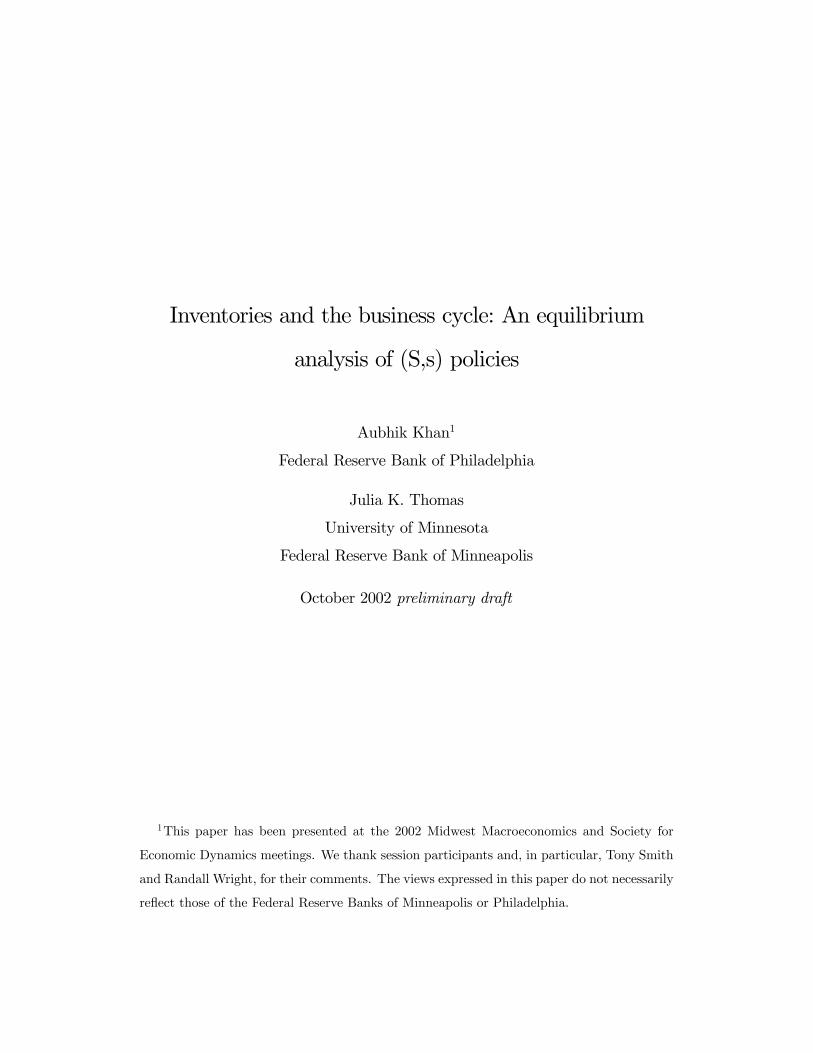
between 1953− 2000. The depreciation rate δ is equal to the average ratio of invest-ment to business capital over the same time period. The distinguishing feature of the

baseline model, relative to the Indivisible Labour Economy of Hansen (1985), is the

presence of intermediate inputs. The single new parameter implied by the additional

factor of production, the share term for intermediate inputs, is set to equal the value

implied by the NBER-CES Manufacturing database, 0.5; this lies in the range esti-

mated by Jorgenson, Gollop and Fraumeni (1987) for U.S. manufacturing over the

years 1947-79. The remaining production parameter, θn, is taken to imply a labour’s

share of output averaging 23 , a value similar to that selected by Hansen (1985) and

Prescott (1986). In terms of preferences, the subjective discount factor, β, is selected

to yield a real interest rate of 4 percent per year in the steady state of the model,

and η is chosen so that average hours worked are 13 of available time. Both values

are taken from Prescott (1986).

We determine the stochastic process for productivity using the Crucini residual

approach described in King and Rebelo (1999). A continuous shock version of the

benchmark model, where log zt+1 = ρ log zt + εt+1 with εt+1 ∼ N¡0, σ2ε

¢, is solved

using linear methods for an arbitrary pair of initial values¡ρ, σ2ε

¢. The linear solution

yields a decision rule for output of the form Yt = πz (ρ) zt + πk (ρ) kt. Rearranging

this solution, data on GDP and capital are then used to infer an implied set of

values for the technology shock series zt. Maintaining the assumption that these

technology shock realizations are generated by a first-order autoregressive process,

the persistence and variance of these implied values yield new estimates of¡ρ, σ2ε

¢.

The process is repeated until these estimates converge. The resulting values for the

persistence and variance of the technology shock process are not uncommon.

4.2 Inventory model

Table 3 lists the baseline calibration of our inventory model. For all parameters

that are also present in the benchmark model, we maintain the same values as there.

This approach to calibrating the inventory model is feasible, as the steady states of

the two model economies, in terms of the capital-output ratio, hours worked, and the

16

shares of the three factors of production, are close.

The two parameters that distinguish the inventory model from the benchmark

are the upper support for adjustment costs (uniformly distributed on [0, B]) and the

storage cost associated with inventories. We determine the upper support as follows.

Using NIPA data, we compute that the quarterly real private nonfarm inventory-to-

sales ratio has averaged 0.714 in the U.S. between 1947 : 1 and 1997 : 4, when the

data series ends. This value lies just above the Ramey and West (1999) average value

across G7 countries of 0.66. Moreover, as noted by these authors, the real series,

in contrast to its nominal counterpart, exhibits no trend. Thus, given the storage

cost σ, we select the parameter B to reproduce this average inventory-to-sales ratio

in our model. The storage cost is difficult to identify in the data; for our baseline

calibration of the model, it is set to equal the rate of depreciation on capital. Given

σ = δ, the upper support of the cost distribution is calibrated at B = 0.204. Higher

storage costs raise the cost of holding inventories and thus require higher adjustment

costs, effectively a larger value for B, to match the measured inventory-sales ratio.

5 Numerical method

(S, s) models of inventory accumulation are rarely examined in equilibrium. As

these models are characterized by an aggregate state vector that includes the distri-

bution of the stock of inventory holdings across firms, computation of equilibrium is

nontrivial. Our solution algorithm involves repeated application of the contraction

mapping implied by (6), (7), (8) and (9) to solve for final goods firms’ start-of-period

value functions V , given the price functions p(z,Ξ), ω(z,Ξ) and q(z,Ξ) and the laws

of motion implied by Γ and (πij). This recursive approach is complicated in two

ways, as discussed below.

First, the nonconvex factor adjustment here requires that we solve for firms’

decision rules using nonlinear methods. This is because firms at times find themselves

with a very low stock of intermediate inputs relative to their production-time target,

but a sufficiently high adjustment cost draw that they are unwilling to replenish

17

their stock in the current period. At such times, they will exhaust their entire stock

in production, deferring adjustment until the beginning of the next period, before

further production. Thus, a non-negativity constraint on inventory holdings binds

occasionally, and firms decision rules are nonlinear and must be solved as such. This

we accomplish using multivariate piecewise polynomial splines, adapting an algorithm

outlined in Johnson (1987). In particular, our splines are generated as the tensor

product of univariate cubic splines, with one of these corresponding to each argument

of the value function.15 We apply spline approximation to V and E1, using a multi-

dimensional grid on the state vector for these functions.

Second, equilibrium prices are functions of a large state vector, given the presence

of the distribution of final goods firms in the endogenous aggregate state vector, Ξ =

(K 0, µ0). For computational feasibility, we assume that agents use a smaller object

to proxy for the distribution in forecasting the future state and thereby determining

their decisions rules given current prices. In choosing this proxy, we extend the

method applied in Khan and Thomas (2002), which itself applied a variation on the

method of Krussel and Smith (1998). In particular, we approximate the distribution

in the aggregate state vector with a vector of moments, m = (m1, ...,mI), drawn

from the distribution. In our work involving discrete heterogeneity in production,

we find that sectioning the distribution into I equal-sized partitions and using the

conditional mean of each partition is very efficient in that it implies small forecasting

errors.

The solution algorithm is iterative, applying one set of forecasting rules to generate

decision rules that are used in obtaining data upon which to base the next set of

forecasting rules. In particular, given I, we assume functional forms that predict

next period’s endogenous state (K 0,m0), and the prices p and pq, as functions of the

current state, K 0 = bΓK ¡z,K,m;χKl¢, m0 = bΓm (z,K,m;χml ), p = bp ¡z,K,m;χpl

¢and pq = bpq ¡z,K,m;χpql

¢, where χKl , χ

ml , χ

pl , and χpql are parameter vectors that

are determined iteratively, with l indexing these iterations. For the class of utility

functions we use, the wage is immediate once p is specified; hence there is no need to

15For additional details, see Khan and Thomas (2002).

18

assume a wage forecasting function.

For any I, bΓK , bΓm, bp, and bpq, we solve for V on a grid of values for (s; z,K,m).

Next, we simulate the economy for T periods, recording the actual distribution of final

goods firms, µt, at the start of each period, t = 1, . . . , T . To determine equilibrium

in each period, we begin by calculating mt using the actual distribution, µt, and

then use bΓK and bΓm to specify expectations of Kt+1 and mt+1. This determines

βNzPj=1

πijw (zj ,Kt+1,mt+1) and βNzPj=1

πijV (s0; zj ,Kt+1,mt+1) for any s0. Given the

second function, the conditional expected continuation value associated with any level

of inventories, we are able to determine s∗ (z,K,m) and ξ (s;K,m), hence recovering

the decisions of final goods firms and the implied next period distribution, given

any values for p and q. Given any p, the equilibrium q is solved to equate the

intermediate input producer’s supply, x(K; z,Ξ), to the demand generated by final

goods firms.16 The equilibrium output price, p(z,Ξ;χKl , χml , χ

pl , χ

pql ), is that which

generates production of the final good such that, given C = 1p , the residual level of

investment, Yt−Ct, implies a level of capital tomorrow, Kt+1 = (1− δ)Kt+Yt−Ct,

that satisfies the restriction in (5). Finally, (18) and (19) determine the distribution

of final goods firms over inventory levels for next period, µt+1. With the equilibrium

Kt+1 and µt+1, we move into the next date in the simulation, again solving for

equilibrium, and so forth. Once the simulation is completed, the resulting data,

(pt, ptqt,Kt,mt)Tt=1, are used to re-estimate

¡χKl , χ

ml , χ

pl , χ

pql

¢using OLS.

We repeat this two-step process, first solving for V given¡χKl , χ

ml , χ

pl , χ

pql

¢, next using

our solution for firms’ value functions to determine equilibrium decision rules over a

simulation, storing the equilibrium results for (pt, ptqt,Kt,mt)Tt=1, and then updating¡

χKl+1, χml+1, χ

pl+1, χ

pql+1

¢, until these parameters converge. The number of partition

means used to proxy for the distribution µ, I, is increased until agents’ forecasting

rules are sufficiently accurate.

16This demand depends on the target inventory level s∗ (z,K,m), the start-of-period distribution

of firms µ(s), and the adjustment thresholds of each firm type ξ (s;K,m).

19

5.1 Forecasting functions

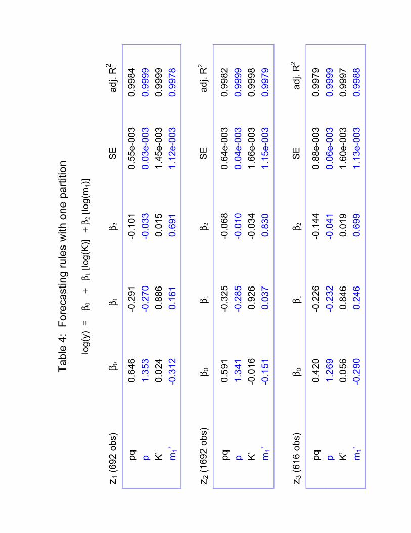
Table 2 displays the actual forecasting functions used for the baseline inventory

model, that in which the model’s inventory-sales ratio matches its measured counter-

part when averaged over the simulation. We use a log-linear functional form for each

forecasting rule that is conditional on the level of productivity, zi, i = 1, . . . ,Nz.17 In

the results reported here, I = 1. This means that, alongside z and K, only the mean

of the current distribution of firms over inventory levels, start-of-period aggregate

inventory holdings, is used by agents to forecast the relevant features of the future

endogenous state. This degree of approximation would be unacceptable if it yielded

large errors in forecasts. However, table 2 shows that, for each of the three values of

productivity, the forecast rules for prices and both elements of the approximate state

vector are extremely accurate. The standard errors across all regressions are small,

and the R-squares are high, all above 0.997.18

In that they provide a description of the behavior of equilibrium prices and the

laws of motion for capital and inventories, the regressions in table 2 also offer some

insight into the impact of inventories on the model. In particular, note that there is

relatively little impact of inventories, m1, on the valuation of current output, p, and

capital, K. Inventories have somewhat larger influence in determining the price of

intermediate inputs and, of course, in forecasting their own future value.

17We have tried a variety of alternatives including adding higher-order terms and a covariance

term. None of these significantly altered the forecasts used in the model. In future we plan to assess

I = 2 for robustness. We were unable to complete this experiment in the current draft because

it implies 5−dimensional value functions, which given our nonlinear method, implies substantialadditional computing cost.18 In evaluating the standard errors, it may be useful to note that the means of p, pq, K and m1

are 3.640, 1.786, 1.239 and 0.4323 respectively.

20

6 Results

6.1 Steady state

Suppressing stochastic changes in the productivity of intermediate goods pro-

ducers, the sole source of uncertainty in our model, table 5 presents the steady state

behavior of final goods firms. This illustrates the mechanics of our generalized (S,s)

inventory adjustment and its consequence for the distribution of production across

firms.

In our baseline calibration, where B = 0.204, there are 5 levels of inventories

identifying firms. This beginning of period distribution is in columns 1 − 5, whilethe first column, labelled adjustors, lists those firms from each of these groups that

undertake inventory adjustment prior to production.

The inventory level selected by all adjusting firms, referred to above as the target

value s∗, is 1.219 in the steady state. Firms that adjusted their inventory holdings

last period, those in column 1, begin the current period with 0.831 units of the inter-

mediate input. Given their relatively high stock of inputs they are unwilling to suffer

substantial costs of adjustment and, as a result, their probability of adjustment is

low, 0.036. The majority of such firms, then, do not undertake inventory adjustment.

These firms use 0.327, almost 40 percent, of their available stock of intermediate

input in current production.

As inventory holdings decline with the time since their last order, firms are willing

to accept larger adjustment costs as they move from group 1 across the distribution

to group 5. Thus, their probability of undertaking an order rises as their inventory

holdings decline, and the model exhibits a rising adjustment hazard in the sense

of Caballero and Engel (1999). Firms optimally pursue generalized (S, s) inventory

policies, undertaking factor adjustment stochastically, and the probability of an in-

ventory adjustment rises in the distance between the current stock and the target

level associated with adjustment.

The steady state table exhibits evidence of some precautionary behavior among

final goods firms, as they face uncertainty about the length of time until they will

21

next undertake adjustment. First, while the representative firm in the benchmark

model orders exactly the amount of inputs it will use in current production, 0.31,

ordering firms in the baseline inventory economy prepare for the possibility of lengthy

delays before the next order, selecting a much higher production-time stock, 1.22.

Next, as these firms’ inventory holdings decline, the amount of intermediate inputs

used in production falls, as does employment and production. The intermediate

input-to-labour ratio also falls, as firms substitute labour for the scarcer factor of

production. However, the fraction of inventories used in production actually rises

until, for firms with very little remaining stock, those in column 4, the entire stock is

exhausted. Nonetheless, firms’ ability to replenish their stocks prior to production in

the next period implies that, even here, the adjustment probability is less than one.

However, for the 0.062 firms that begin the period with zero input holdings, all adjust

prior to production, adopting the common target. Hence, while the columns labelled

1 − 5 reflect the beginning of period distribution of firms over inventory levels, thefinal column is not relevant in the production-time distribution. The first column,

reflecting the behavior of adjusting firms, replaces it in production.

6.2 Business cycles

6.2.1 Inventory investment and final sales

Our first goal was to generalize an equilibrium business cycle model to reproduce

the empirical regularities involving inventory investment. This we saw as a necessary

first step in developing a model useful for analyzing the role of inventories in the

business cycle. Table 6 presents our inventory model’s predictions for the volatility

and cyclicality of GDP, final sales, inventory investment and the inventory-to-sales

ratio. These predictions, derived from model simulations, are contrasted with the

corresponding values taken from postwar U.S. data. All series are Hodrick-Prescott

filtered.

Table 6A reports percentage standard deviations for each series relative to that

22

of GDP.19 Contemporaneous correlations with GDP are listed in table 6B. Together,

the two panels of table 6 establish that our baseline inventory model is successful

in reproducing both the procyclicality of net inventory investment and the higher

variance of production when compared to final sales. Further, this simple model with

nonconvex factor adjustment costs as the single source of inventory accumulation is

able to explain 52 percent of the measured relative variability of net inventory invest-

ment. Finally, from table 6B, note that the inventory-to-sales ratio is countercyclical

in our model, as in the data. We take these results to imply that the predictions

of the model are sufficiently accurate to validate its use in exploring the impact of

inventory investment on aggregate fluctuations.

Certainly, there are differences between the model and data. The most pro-

nounced departures in the model are its understated variability of inventory invest-

ment and its exaggerated counter-cyclicality of the ratio of inventories to final sales.

However, the degree of procyclicality in inventory investment, as well as the excess

variability of production over sales, are well reproduced by the model. The latter

arises from the positive correlation between inventory investment and final sales,

0.781 in our model.

6.2.2 Aggregate implications of inventory investment

In tables 7A and 7B, we begin to assess the role of inventories in the business

cycle using our model. The first row of each table presents results for the benchmark

model without inventories, the second row reports the equivalent moment from the

inventory model. The most striking aspect of this comparison is the broad similarity

in the dynamics of the two model economies. At first look, the introduction of inven-

tories into an equilibrium business cycle model does not appear to alter the model’s

predictions for the variability or cyclicality of production, consumption, investment

or total hours in any substantial way. The differences that do exist are quantita-

tively minor, and the qualitative features of the equilibrium business cycle model are

19The exception is net inventory investment, which is detrended relative to GDP, as described in

footnote 7.

23

unaltered. The familiar features of household consumption smoothing continue to

imply an investment series that is substantially more variable than output, allowing

a consumption series that is less variable than output. Furthermore, the variability of

total hours remains lower than that of production. Likewise, table 7B shows little dif-

ference in the contemporaneous correlations with output across the two models. The

most apparent divergence appears with respect to capital, which is less procyclical in

the inventory economy due to its reduced responsiveness of final sales.

One noteworthy distinction between the benchmark business cycle economy and

the baseline inventory economy is the latter’s higher standard deviation of GDP. We

introduced our paper by discussing the view that inventories exacerbate fluctuations

in production. Table 7A appears to provide some equilibrium substantiation for this

view. However, the increase in GDP volatility is rather small, only 0.092 percentage

points. Given that the level of inventories in our model is calibrated to reproduce their

intensity of use in the US economy, we may conclude from this that inventories are of

minimal consequence in amplifying fluctuations in production. Furthermore, Table

7A shows that the variability of final sales actually falls in the presence of inventory

investment.20 This is further evident in the relative variability of consumption and

investment, both of which are reduced in the inventory model. The variability of total

hours worked, by contrast, is raised relative to the economy without inventories.

Tables 8A and 8B provide additional observations that may help in explaining

the differences across models, particularly with regard to the hours series. Note that

the inventory economy’s higher variance in total hours arises entirely from increased

variability in hours worked in the intermediate goods sector, Ninter. Moreover, shifts

toward more labor-intensive production of intermediate inputs, (evidenced by the

countercyclical K/Ninter series), are stronger in the inventory model, partly because

procyclical inventory investment diverts some resources away from the production of

final goods, and hence from investment in capital. Hours worked in the final goods

sector, Nfinal, are actually less variable in the presence of inventories. In both model

20Recall that final sales in the benchmark model is equivalent to production, given the absence of

inventory investment.

24

economies, the use of intermediate inputs per worker is procyclical, as technology

shocks to the intermediate goods sector make the relative price of intermediate in-

puts, q, countercyclical. However, this effect is weaker in the inventory economy;

consequently M/Nfinal is less variable and less procyclical there.

Inventories exist in our model because of fixed adjustment costs. These costs

imply state-dependent (S, s) adjustment policies for final goods firms maintaining

stocks of intermediate intputs. In table 5, we saw that only about one-third of firms

actively adjust their inventories in any given period in the steady state.21 Staggered

factor adjustment dampens the average response of final goods firms to changes in

relative prices associated with the business cycle. As a result, the response in final

goods is dampened relative to the benchmark economy, as reflected in the reduced

variability of consumption, investment and final sales, the sum of these two series.

One consequence of this dampened response is that efforts to increase production of

intermediate inputs in response to a positive productivity shock must rely relatively

more on employment, and less on capital. This makes hours worked in the intermedi-

ate goods sector rise by more in such times than in the benchmark economy without

inventories. This appears to explain the increased variability of hours worked, both

in total and in the intermediate goods sector, and the reduced variability of final

sales. Moreover, as productivity shocks are persistent, part of the raised level of

intermediate inputs delivered to adjusting final goods firms is retained by these firms

as inventory investment, which increases in times of high productivity. Because this

retained portion does not immediately translate into higher production of final out-

put, fluctuations in final sales are dampened. Thus, inventory accumulation implies

a second restraint on the volatility of final sales, beyond that directly implied by the

scarcity of inputs among those firms deferring orders.

In concluding this section, we emphasize what we see as a central result of our

study. All else equal, a positive covariance between final sales and inventory invest-

21However, the rate of adjustment is procyclical in the inventory model, and relatively variable.

Its percentage standard deviation relative to output is 0.941, and the contemporaneous correlation

between the number of firms undertaking adjustment and GDP is 0.961.

25

ment must increase the variability of production. However, as was clear in table 7

and in the discussion above, final sales are not exogenous; they are affected by the

introduction of inventories. Our general equilibrium analysis suggests that noncon-

vex costs, the impetus for the accumulation of stocks of intermediate inputs, tend to

dampen changes in final output. The percentage standard deviation of final sales,

1.35 for the benchmark model, falls to 1.28 when inventories are present in the econ-

omy. This reduction in final sales variability largely offsets the effects of introducing

inventory investment for the variance of total production.

6.2.3 Inventory-to-sales ratio

The results of the previous section indicate that, when nonconvex costs induce

firms to hold inventories, cyclical fluctuations in final goods production are reduced

relative to those that would occur if the costs could be eliminated. It then follows

that higher levels of these costs, increasing the level of inventories relative to final

output in the economy, should further mitigate the business cycle. In this section,

we explore this possibility by increasing the upper support of the cost distribution,

B, from the baseline value of 0.204 to 0.3. This pushes the average inventory-to-

sales ratio up by approximately 15 percent to 0.83. We interpret this change as a

rise in the average level of inventory holdings in the economy. Maintaining all other

parameters, we contrast the behavior of this high inventory economy to the baseline

inventory economy where the inventory-to-sales ratio is 0.714, the average quarterly

value observed between 1947.1 and 1997.4 in the data.

Table 9A reveals that higher inventory levels are associated with a fall in the

variability of consumption, investment and final sales, and also a reduction in the

percentage standard deviation of GDP.22 Moreover the volatility of hours worked

in the intermediate goods sector rises, though, with lesser responses in intermediate

input usage, the decline in the variability of hours in the final goods sector more than

offsets any impact of this increase on the standard deviation of total hours worked.

22Although the relative volatility of consumption rises in the high inventory economy, the percent

standard deviation in consumption, falls slightly.

26

As we have argued, nonconvex adjustment costs tend to dampen the response of firms

to the exogenous changes in productivity that drive the business cycle, both because

of the staggered nature of their factor adjustments and because of their reluctance

to deplete or over-accumulate their input stocks in response to shocks. As a result,

larger average adjustment costs associated with a higher average inventory-to-sales

ratio necessarily imply less severe business cycles.

The increased prevalence of inventories in the model economy certainly raises the

variability of net inventory investment. Its standard deviation relative to GDP is

now much closer, at 0.222, to the measured value in the data, 0.271. However, the

volatility of final sales declines, its relative standard deviation falling closer to its

empirical counterpart, 0.824. As a result the positive correlation between final sales

and net inventory investment, 0.702, fails to raise the variance of production. GDP

volatility actually falls relative to the economy with the lower inventory-to-sales ratio.

7 Concluding remarks

In the preceding pages, we generalized an equilibrium business cycle model to

allow for endogenous (S, s) inventories of an intermediate input in final goods produc-

tion. We showed that our calibrated baseline model of inventories is able to account

for the procyclicality of inventory investment, the higher variance of production rela-

tive to sales, the countercyclicality of the inventory-to-sales ratio (qualitatively), and

approximately one-half of the relative variability of net inventory investment. Using

this model to assess the role of inventory investment in the aggregate business cy-

cle, we found that the inventory economy exhibits a business cycle that is broadly

similar to that of its benchmark counterpart without inventory investment. How-

ever, the adjustment costs that induce inventory holdings also dampen fluctuations

in final output, which substantially limits the effects of inventory accumulation for

the variability of total production, despite the positive correlation between final sales

and inventory investment. Reexamining the model’s predictions in the presence of

higher adjustment costs, we have seen that an increased presence of inventories in

27

the economy actually reduces aggregate fluctuations.

In future work, we will consider additional sources of fluctuations. This is par-

ticularly important, as we know that the source of shocks has proved critical for the

implications of the traditional inventory model. The technology shock studied here

is ordinarily interpreted as a supply shock, since it raises productivity in the interme-

diate goods sector. However, it may also be viewed by final goods firms as a demand

shock, as it is essentially a rise in the relative price of their output. Thus, in our

multi-sector general equilibrium model, the demand or supply origin of the current

disturbance appears ambiguous. Nonetheless, when fluctuations arise from demand

shocks that do not directly alter the relative price of intermediate inputs, the cyclical

role of inventories may differ from that seen here.

28

References

[1] Blinder, A. S. (1990) Inventory theory and consumer behavior, University of

Michigan Press.

[2] Blinder A. S. and L. J. Maccini (1991) ‘Taking stock: a critical assessment of

recent research on inventories’ Journal of Economic Perspectives 5, 73-96.

[3] Caballero, R. J. and E. M. R. A. Engel (1999) ‘Explaining investment dynamics

in U.S. manufacturing: a generalized (S, s) approach’ Econometrica 67, 783-826.

[4] Christiano, L. J. (1988) ‘Why does inventory investment fluctuate so much?’

Journal of Monetary Economics 21: 247-80.

[5] Coen-Pirani, D. (2002) ‘Microeconomic inventory behavior and aggregate inven-

tory dynamics’ GSIA working paper, Carnegie-Mellon University.

[6] Fisher, J. D. M. and A. Hornstein (2000) ‘(S, s) inventory policies in general

equilibrium’ Review of Economic Studies 67: 117-145.

[7] Fitzgerald, T. J. (1997) ‘Inventories and the business cycle: an overview’ Eco-

nomic Review 33 (3): 11-22, Federal Reserve Bank of Cleveland.

[8] Hall, G. and J. Rust (1999) ‘An empirical model of inventory investment by

durable commodity intermediaries’ Yale University working paper.

[9] Hansen, G. D., (1985) ‘Indivisible labor and the business cycle’ Journal of Mon-

etary Economics 16, 309-327.

[10] Hornstein, A. (1998) ‘Inventory investment and the business cycle’ Economics

Quarterly 84, 49-71, Federal Reserve Bank of Richmond.

[11] Humphreys, B. R., L. J. Maccini, and S. Schuh (2001) ‘Input and output inven-

tories’ Journal of Monetary Economics 47: 347-375.

29

[12] Johnson, S. A. (1989) Spline approximation in discrete dynamic programming

with application to stochastic multi-reservoir systems Unpublished dissertation

(Cornell, Ithaca, NY).

[13] Kahn, J. A. (1987) ‘Inventories and the volatility of production’ American Eco-

nomic Review 77, 667-679.

[14] Kahn, J., M. McConnell and G. Perez-Quiros (2001) ‘Inventories and the infor-

mation revolution: implications for output volatility’ Federal Reserve Bank of

New York working paper (2001).

[15] Khan A.and J. K. Thomas, (2002) ‘Nonconvex factor adjustments in equilib-

rium business cycle models: do nonlinearities matter?’ Journal of Monetary

Economics forthcoming.

[16] King, R. G. and S. T. Rebelo, (1999) ‘Resuscitating real business cycles’ in: M.

Woodford and J. Taylor, eds., Handbook of Macroeconomics IB (Elsevier Science,

Amsterdam): 927 - 1007.

[17] Krusell, P. and A. A. Smith Jr. (1997) ‘Income and wealth heterogeneity, portfo-

lio choice, and equilibrium asset returns’ Macroeconomic Dynamics 1, 387-422.

[18] Krusell, P. and A. A. Smith Jr. (1998) ‘Income and wealth heterogeneity in the

macroeconomy’ Journal of Political Economy 106, 867-896.

[19] Kydland, F. and E. C. Prescott (1982) ‘Time to build and aggregate fluctuations’

Econometrica 50, 1345 - 1370.

[20] Prescott, E. C. (1986), ‘Theory ahead of business cycle measurement’ Quarterly

Review 10, Federal Reserve Bank of Minneapolis: 9-22.

[21] Ramey, V. A., (1991) ‘Nonconvex costs and the behavior of inventories’ Journal

of Political Economy 99, 306-334.

30

[22] Ramey, V. A. and K. D. West. (1999) ‘Inventories’ in: M. Woodford and J.

Taylor, eds., Handbook of Macroeconomics IB. (Elsevier Science, Amsterdam),

863 - 922.

[23] Rogerson, R., (1988) ‘Indivisible labor, lotteries and equilibrium’ Journal of

Monetary Economics 21, 3-16.

31

Tabl

e 1:

GD

P, F

inal

sal

es a

nd in

vent

orie

s

G

DP

Fina

l Sal

es

Net

Inve

ntor

y In

vest

men

t In

vent

ory-

to-S

ales

perc

ent s

tand

ard

devi

atio

n re

lativ

e to

GD

P 1.

675

0.82

4 0.

271

0.72

1

corre

latio

n w

ith G

DP

1.00

0 0.

951

0.65

8 -0

.396

corre

latio

n w

ith N

II 0.

658

0.41

7 1.

000

-0.1

74

Dat

a ar

e qu

arte

rly, 1

954.

1 –

2001

.2.

All s

erie

s ar

e H

odric

k-Pr

esco

tt fil

tere

d. G

DP

and

final

sal

es a

re re

porte

d as

sta

ndar

d de

viat

ions

, and

net

in

vent

ory

inve

stm

ent i

s de

trend

ed re

lativ

e to

GD

P.

Tabl

e 2:

Sec

tora

l dis

tribu

tion

of p

rivat

e no

n-fa

rm in

vent

orie

s

perc

enta

ge o

f tot

al

stoc

k of

inve

ntor

ies

STD

(inve

ntor

y in

vest

men

t) co

rrela

tion(

inve

ntor

y in

vest

men

t, G

DP)

M

anuf

actu

ring

37

0.

14

0.65

finis

hed

good

s 13

w

ork

in p

roce

ss

12

mat

eria

ls &

sup

plie

s 12

Trad

e

reta

il 26

0.

12

0.32

who

lesa

le

26

0.09

0.

35

Oth

er

11

C

olum

n 3,

the

perc

enta

ges

of th

e to

tal s

tock

of i

nven

torie

s, is

take

n fro

m R

amey

and

Wes

t (19

99),

page

869

, tab

le 4

.

Ta

ble

3: B

asel

ine

calib

ratio

n

β η

α θ m

θ n

σ

δ A

B ρ z

σ ε

0.99

0 2.

185

0.25

2 0.

500

0.29

3 0.

019

0.01

9 0.

000

0.20

4 0.

981

0.01

4

Ta

ble

4: F

orec

astin

g ru

les

with

one

par

titio

n

lo

g(y)

=

β0

+

β 1 [l

og(K

)] +

β2 [

log(

m1)

] z 1

(692

obs

)

β 0

β 1

β 2

SE

adj.

R2

pq

0

.646

-0.2

91

-0

.101

0.55

e-00

3

0.99

84

p

1

.353

-0.2

70

-0

.033

0.03

e-00

3

0.99

99

K’

0

.024

0.8

86

0

.015

1.45

e-00

3

0.99

99

m1’

-0.3

12

0

.161

0.6

91

1.

12e-

003

0.

9978

z 2

(169

2 ob

s)

β 0

β 1

β 2

SE

adj.

R2

pq

0.5

91

-0

.325

-0.0

68

0.

64e-

003

0.

9982

p

1.3

41

-0

.285

-0.0

10

0.

04e-

003

0.

9999

K’

-0

.016

0.9

26

-0

.034

1.66

e-00

3

0.99

98

m

1’

-0

.151

0.0

37

0

.830

1.15

e-00

3

0.99

79

z 3

(616

obs

)

β 0

β 1

β 2

SE

adj

. R2

pq

0.4

20

-0

.226

-0.1

44

0.

88e-

003

0.

9979

p

1

.269

-0.2

32

-0

.041

0.06

e-00

3

0.99

99

K’

0.0

56

0

.846

0.0

19

1.

60e-

003

0.

9997

m1’

-0.2

90

0

.246

0.6

99

1.

13e-

003

0.

9988

Ta

ble

5: D

istri

butio

n of

fina

l goo

ds fi

rms

in s

tead

y-st

ate

ad

just

ors

1 2

3 4

5

µ(s)

: sta

rt-of

-per

iod

dist

ribut

ion

0.

279

0.26

9 0.

232

0.15

8 0.

061

s: s

tart-

of-p

erio

d in

vent

orie

s

0.83

3 0.

504

0.23

8 0.

055

0.00

0

α(s)

: fra

ctio

n ad

just

ing

0.

036

0.14

0 0.

318

0.61

1 1.

000

s 1: p

rodu

ctio

n-tim

e in

vent

orie

s 1.

221

0.83

3 0.

504

0.23

8 0.

055

0.00

0

m: i

nter

med

iate

inpu

t 0.

389

0.32

8 0.

266

0.18

3 0.

055

0.00

0

n: la

bour

0.

186

0.16

5 0.

142

0.10

9 0.

047

0.00

0

y: p

rodu

ctio

n 0.

365

0.32

8 0.

287

0.22

3 0.

096

0.00

0

m/n

2.

091

1.99

0 1.

871

1.67

7 1.

176

n/a

prod

uctio

n sh

are

0.27

9 0.

269

0.23

2 0.

158

0.06

1 0.

000

Ta

ble

6: In

vent

ory

dyna

mic

s fo

r the

bas

elin

e m

odel

G

DP

Fina

l Sal

es

Net

Inve

ntor

y In

vest

men

t In

vent

ory/

Sale

s

A: p

erce

nt s

tand

ard

devi

atio

ns re

lativ

e to

GD

P da

ta

1.67

5 0.

824

0.27

1 0.

721

base

line

inve

ntor

y 1.

441

0.88

5 0.

141

0.92

1

B: c

onte

mpo

rane

ous

corre

latio

ns w

ith G

DP

data

0.95

1 0.

658

-0.3

96

base

line

inve

ntor

y

0.99

6 0.

834

-0.9

64

Tabl

e 7:

Bas

elin

e in

vent

ory

mod

el

G

DP

Fina

l Sal

es

Con

sum

ptio

n In

vest

men

tTo

tal H

ours

Cap

ital

A:

per

cent

sta

ndar

d de

viat

ions

rela

tive

to G

DP

benc

hmar

k 1.

349

1.00

0 0.

538

6.65

8 0.

501

0.41

8

base

line

inve

ntor

y 1.

441

0.88

5 0.

471

6.32

3 0.

575

0.40

7

B: c

onte

mpo

rane

ous

corre

latio

ns w

ith G

DP

benc

hmar

k

1.00

0 0.

965

0.96

1 0.

959

0.15

8

base

line

inve

ntor

y

0.99

6 0.

939

0.96

8 0.

964

0.12

7

Tabl

e 8:

Bas

elin

e in

vent

ory

mod

el c

ontin

ued

N

inte

r N

final

X

M

q K

/ Nin

ter

M /

Nfin

al

A: p

erce

nt s

tand

ard

devi

atio

ns re

lativ

e to

GD

P be

nchm

ark

0.50

1 0.

501

1.72

1 1.

721

0.72

3 0.

693

1.25

8

base

line

inve

ntor

y 0.

696

0.44

1 1.

765

1.52

7 0.

667

0.85

3 1.

128

B:

con

tem

pora

neou

s co

rrela

tions

with

GD

P be

nchm

ark

0.95

9 0.

959

0.99

9 0.

999

-0.9

93

-0.5

99

0.98

4

base

line

inve

ntor

y 0.

955

0.96

2 0.

998

0.99

1 -0

.981

-0

.719

0.

966

Ta

ble

9: H

igh

inve

ntor

y m

odel

G

DP

FS

C

I H

ours

Nin

ter

Nfin

al

M

NII

K/N

inte

rM

/Nfin

al

A: p

erce

nt s

tand

ard

devi

atio

ns re

lativ

e to

GD

P ba

selin

e in

vent

ory

1.44

1 0.

885

0.47

1 6.

323

0.57

5 0.

696

0.44

1 1.

527

0.14

1 0.

853

1.12

8

high

in

vent

ory

1.38

2 0.

831

0.48

5 5.

560

0.56

0 0.

739

0.36

6 1.

478

0.22

2 0.

906

1.14

1

B: c

onte

mpo

rane

ous

corre

latio

ns w

ith G

DP

base

line

inve

ntor

y

0.99

6 0.

939

0.96

80.

964

0.95

5 0.

962

0.99

10.

834

-0.7

19

0.96

6

high

in

vent

ory

0.

988

0.93

9 0.

963

0.95

9 0.

936

0.96

8 0.

981

0.80

4 -0

.742

0.

960