1

HOUSEHOLD SCHOOLING DECISIONS

IN RURAL PAKISTAN*

by

Yasuyuki Sawadaa, b ** and Michael Lokshinb

a Department of Advanced Social and International Studies, University of Tokyo, Komabab Development Research Group, World Bank

Abstract

Field surveys were conducted in twenty-five Pakistani villages exclusively for this paper. By integratingfield observations, economic theory, and econometric analysis, this paper investigates the sequentialnature of educational decisions. The full-information maximum likelihood (FIML) estimation of thesequential schooling decision model uncovers important dynamics of the gender gap in education,transitory income and wealth effects, and intrahousehold resource allocation patterns. We find, amongthings, that there is a high educational retention rate, conditional on school entry, and that schoolingprogression rates become comparable between male and female students at a high level of education.Moreover, a household’s human and physical assets and income changes affect child education patternssignificantly. These findings are consistent with the theoretical implications of optimal schoolingbehavior under binding credit constraints. Finally, we found serious supply-side constraints on femaleprimary education in the villages, suggesting the importance of supply-side policy interventions inPakistan’s primary education.

Keywords: sequential schooling decisions; income shocks; birth-order effects; supply-side constraints

* This research is financially supported by the Scientific Research Fund of the Japanese Ministry ofEducation, the Foundation for Advanced Studies on International Development, and the MatsushitaInternational Foundation. We would like to thank Sarfraz Khan Qureshi and Ghaffar Chaudhry, theformer director and the joint director, respectively, of the Pakistan Institute of Development Economics;Punjab village enumerators Azkar Ahmed, Muhammad Azhar, Anis Hamudani, and Ali Muhammad; andNWFP village enumerators Aziz Ahmed, Abdul Azim, Asad Daud, and Lal Muhammad for support offield surveys. Suggestions and guidance from Harold Alderman, Takeshi Amemiya, Jere Behrman,Marcel Fafchamps, Nobu Fuwa, Anjini Kocher, Sohail Malik, Jonathan Morduch, Pan Yotopoulos, andseminar participants at Stanford University are gratefully acknowledged.

** Corresponding author, email: sawada@stanfordalumni.org.

2

1 Introduction

The recent revival of economic growth theory has renewed interest in the nexus of human capital

investment and growth (Barro and Sala-i-Martin 1995). Studies across countries show that human capital

investments in Pakistan are performing poorly: the school enrollment rate is low, school dropouts are

widespread, and there is a distinct gender gap in education (Behrman and Schneider 1993; Sawada 1997).

Theory suggests that the low level of education in Pakistan may have a strong negative effect on the

country’s long-term macroeconomic growth. The microeconomic behavior of Pakistani households

should underlie such a macroeconomic movement, involving the interplay of parental objectives and

constraints faced by the households.

However, human capital is accumulated through a complicated decision-making process. The

educational outcome is typically represented by years of completed schooling, which is a stock rather

than flow variable. In this case, the current outcome depends not only on the current decision but also on

past decisions. Therefore, general reduced form solutions will include the entire history of exogenous

influences (Strauss and Thomas 1995, 1974-75). Yet, such historical data on individual and household

characteristics are rarely available. Because appropriate data are typically missing, the dynamic aspects

of education are ignored in most of the reduced form empirical literature. However, even if we have the

data that theory requires, introducing dynamics by having the current period’s outcome depend on past

outcomes complicates the estimation procedure.

This paper attempts to overcome these two issues in the existing literature on education by

making two important contributions. First, to examine explicitly the dynamic and sequential aspects of

schooling decisions, we use a unique data set on the whole retrospective history of child education and

household background, which was collected exclusively for this analysis through field surveys in rural

Pakistan. This data collection itself contributes to the literature, shedding light on dynamic aspects of

education. Second, in addition to the data contribution, this paper uses the full-information maximum

likelihood (FIML) method to cope with the complicated estimation procedure of multiple integration of

conditional schooling probability. This method, combined with the unique data set, enables us to estimate

the full sequential model.

The estimation results of sequential schooling probabilities provide new and important insights

on demand for education. In sum, five important findings emerge from our estimation. First, the most

striking feature discovered is the high educational retention rate, conditional on school entry. Second, the

schooling progression rates become comparable between male and female students at a high level of

education. These observations indicate that parents might pick the “winners” for educational

3

specialization and allocate more resources to them, regardless of their gender. Third, we found that this

schooling pattern can be explained partly by physical and human asset ownership and parental income

and health shocks. Fourth, we found gender-specific birth-order effects that suggest resource competition

among siblings. These third and fourth findings are consistent with the theoretical implications of the

optimal educational investment behavior under binding credit constraints. Hence, this paper gives

important new insights for understanding the dynamics of household risk-coping strategies and

educational decisions in developing countries. Finally, we found that the supply side constraints of

education in the village significantly restrict education, especially for females. The last finding suggests

the importance of future research on the supply side management of education.

This paper proceeds as follows: Section 2 describes the key features of human capital

investments in rural Pakistan, which were identified from the field research. Based on initial observations

from the field, Section 3 applies the standard theory of dynamic schooling investment decisions. Based

on the theoretical framework, we derive an econometric model with which we can estimate the

conditional schooling probabilities in Section 4. Section 4 then shows estimation results of the empirical

model. The final section offers conclusions and policy implications.

2 The Key Features Identified in the Field

Our approach follows an iterative process of (1) initial hypothesis, (2) field survey, (3) theory, and (4)

empirical analysis, which is suggested by Townsend (1995). Instead of directly implementing

econometric tests based on an existing well-defined data set, this paper starts with key features of

household behaviors discovered in the field. Modification of data collection was undertaken in the initial

stage, and the standard theory is augmented afterward according to the field observations.

Field surveys were conducted twice to gather information exclusively for this paper. In the first

round of the survey in February through April 1997, the survey team carried out interviews in fourteen

villages of the Fisalabad and Attock districts of Punjab province. Then the second-round surveys were

conducted in eleven villages of the Dir districts of the North-West Frontier Province (NWFP) in

December 1997 through January 1998. Our field surveys covered 203 households in Punjab and 164

households in NWFP. Hence, 367 households were interviewed, and information on a total of 2,365

children was collected.1 The combined data give a complete set of retrospective histories of child

==========================================================

1 The selection of our survey sites was predetermined, since we basically resurveyed the panel households that hadbeen interviewed by the International Food Policy Research Institute (IFPRI) through the Food Security ManagementProject (Alderman and Garcia 1993; Alderman 1996). The initial IFPRI data collection was based on a stratifiedrandom sampling scheme. A detailed description of the procedure of our field surveys is summarized in the

4

schooling, together with household and village level information.

The most striking feature uncovered in the field is the high educational retention rate, conditional

on school entry. According to our survey data, years of schooling averaged 1.6 years for all female

children in the overall sample, whereas they were 6.6 years for male children. On the other hand, for

children who had entered primary school, the average years of schooling become 6.0 years for girls and

8.8.years for boys. These numbers indicate that after entering school, children’s years of schooling

dramatically increase.

To examine the school progression rates in detail at different educational stages, we utilize the

framework of estimating the conditional survival function. The Pakistani education system is composed

of five years of primary education, five years of secondary education, and postsecondary education.2

Educational outcomes can be understood as a result of five sequential schooling decisions. The first

decision is whether to enter primary school (S*1), where S*τ represents schooling time of a child at τ-th

educational stage. For those who attended primary school, the second decision is whether to finish

primary school (S*2). Then the third decision for primary school graduates is whether to continue to

secondary school or stop education at grade five (S*3). For those who entered secondary school, the

fourth decision is whether to stop before grade ten or to graduate from secondary school (S*4). The final

decision is whether to continue beyond secondary school—that is, to enter college, technical, or teaching

school (S*5).3

Let nk denote the number of students whose have completed education of the stage of S*k-1. We

simply used data where S*k-1 is not right-censored at the education level k-1. The set of individuals whose

school attainment is at least S*k-1 is called the risk set at the k-th stage of education, S*k, and thus nk

represents the size of the risk set at the level k. Among nk students, let hk denote the number of children

who have completed education level k, and therefore hk = nk+1. Then, an empirical estimate of the

conditional survival probability at education level k would be hk/nk. This number represents the fraction

of students who go on to a higher stage of education, conditional on the completion of the education level

k-1. Also, this can be interpreted as the sample conditional probability of school continuation to the

education level k.

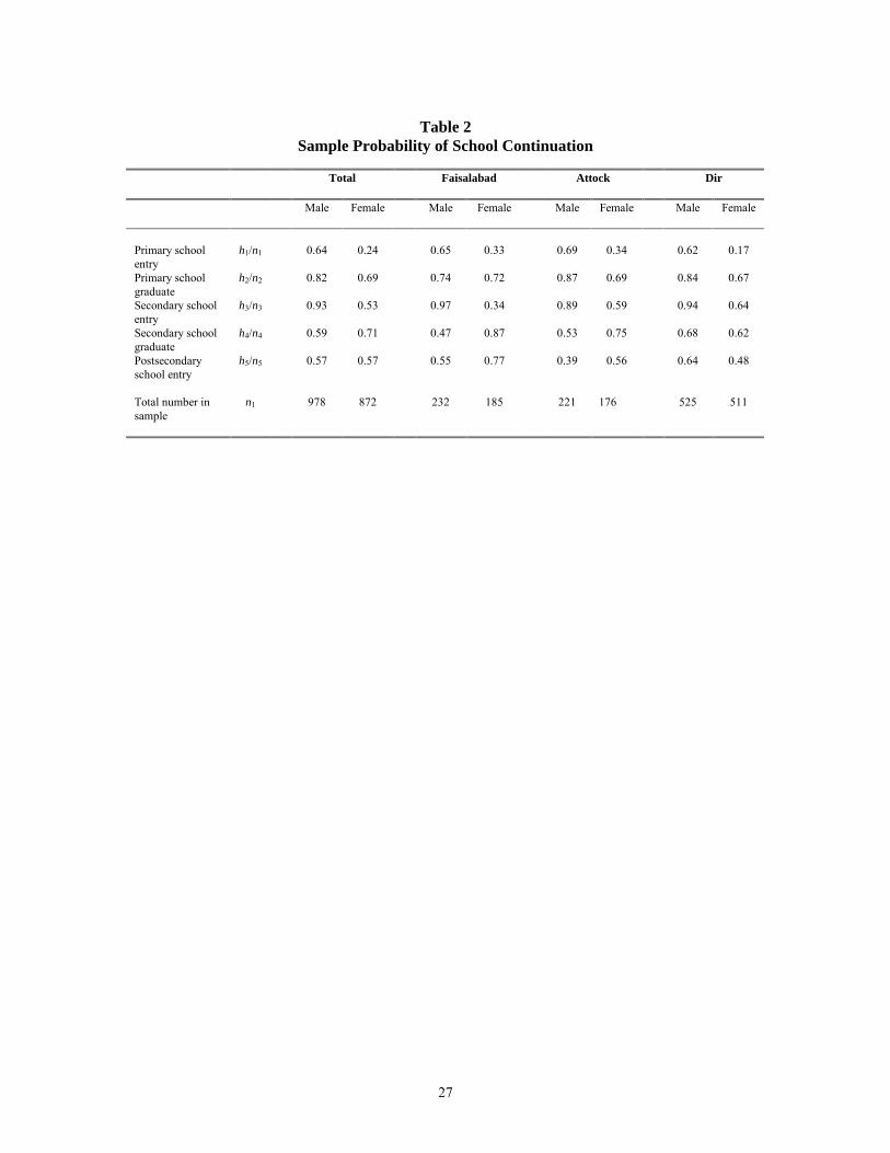
The estimated conditional survival or school continuation probabilities are summarized in Table

2. As we can see in Table 2, the survival rate at the first entry—that is, the probability of ever entering

===========================================================================================================================================================================================

appendix.2 Strictly speaking, secondary education in Pakistan is composed of three years of middle education and two years ofhigh school education.3 We assume that for those who did not enter a primary school, the decision was made when the child was at the ageof six, which is the median age of primary school entry (Table 1). We impose similar assumptions for secondary andpostsecondary education.

5

school—is low both for boys (64 percent) and girls (24 percent). We can also note that the female

conditional schooling probability is less than half of the male conditional probability at primary school

entry. After entering primary school, however, conditional primary school graduation rates become 82

percent and 69 percent for male and female students, respectively. These statistics indicate that after

entering school, the majority of children remain at school. Another interesting finding is that while the

conditional schooling probability is lower for girls than that for boys at primary school entry and

graduation and at secondary school entry, the conditional schooling probabilities after secondary school

entry are consistently higher for females in Punjab province. The gender gap in education eventually

seems to disappear at the higher stages of education.4 This finding indicates an important dynamics of the

gender gap in education, which has not been pointed in the literature.

These basic statistics also suggest substantial differences in the degree of the educational gender

gap among districts. According to Table 2, in the Dir district of NWFP, the conditional survival rates are

consistently lower for females at all stages of the schooling decision. The district differences seem to be

largely due to sociocultural factors. For example, the custom of seclusion of women, purdah, is strictly

maintained in the Dir district. These regional divergences in gender gap in rural Pakistan raise an

important policy issue. Alderman et al. (1995) pointed out that when the government allocates education

expenditures, disadvantaged groups such as girls and children in lagging regions should be targeted to

assure more equitable gains from schooling.

3 The Standard Theory of Educational Investments

Having discussed the key observations in the field, the next step is to formulate a formal model of the

household’s optimal schooling behavior, integrating the key features. A possible interpretation of the

above findings is that parents might pick the “winners” for educational specialization and allocate more

resources to them. As an initial theoretical framework to account for this household behavior, we employ

the two sets of optimal behavioral rules. First, parents decide the intertemporal allocation of resources so

as to maximize the expected total lifetime utility of the family. Second, parents also make a decision on

the allocation of educational resources among children, given the overall resource constraint of the

household.

==========================================================

4 We also estimated the Kaplan-Meier product limit estimator, and the results are available upon request from thecorresponding author. The Kaplan-Meier estimator of survival beyond stage k is the product of survival probabilitiesat k and the preceding periods. Graphing survival probability against sequence k produces a Kaplan-Meier survivalcurve. Again, at the primary school entry level, the school survival rate is much higher for males than for females.The slope of survival function, however, is flatter for females, indicating that gender gap in education becomessmaller at the higher levels of education.

6

We use a standard investment model of education as the benchmark and apply it to the context of

rural Pakistan. The basic setup of our model is based on the seminal works by Levhari and Weiss (1974)

and Jacoby and Skoufias (1997) on human capital investment under uncertainty. In particular, we extend

the Jacoby and Skoufias (1997) model to a generalized form with multiple children. Essentially, risk,

uncertainty, and constraints on insurance and credit influence poor Pakistani households’ investment and

consumption decisions. Therefore, we formalize human capital accumulation in rural Pakistan as

households’ sequential schooling investment decisions under uncertainty and credit constraints.

Suppose a household with n children decides household consumption, C, and schooling for child

i, Si, so as to maximize the household’s aggregated expected utility with concave instantaneous utility

function, U(• ), given the information set at the beginning of time t, Ωt. The information set, Ωt, includes

initial asset ownership and the whole history of household variables. Such a household’s problem can be

represented as follows:

⋅⋅⋅+ +++++

−

=+ t

CnT

CT

CTT

TtT

kkt

k

SCHHHAWCUEMax

itt

Ω ) , ,,,()( 1121111

0,ββ

s.t )1()1()(1

1 ttit

n

ii

Pttt rCSwHYAA +

−−++==

+

[ ] , n, , ieqSfHHn

iititit

Cit

Cit ⋅⋅⋅=++=

=+ 21 ,),(

11

tit

n

ii

Ptt CBSwHYA ≥+−++

=

)1()(1

0 given, are and , ,0 00 ≥≥ TP ABAHB .

In this problem, the objective function includes a concave function, W(• ), of financial bequest and salvage

value of the final stock of the child’s human capital. The parameter β represents a discount factor. The

first constraint is the household’s intertemporal budget constraint. This household’s consumable

resources in each period are composed of assets, A; stochastic parental income, Y, which is a function of

parents’ human capital, HP; and total child income, Σiwi(1-Sit), with wi being the child-specific wage rate.5

Note that a child’s total time endowment is normalized to 1. The second constraint is the human capital

accumulation equation. The human capital production function, f(• ), includes the variable q, which

represents the school supply side-effect, the gender gap, and subjective factors. Among others, the

variable q is a function of a time-invariant gender indicator variable that takes 1 if the child is female and

==========================================================

5 We assume that a child’s schooling does not change the child wage rate immediately, and accumulated humancapital, HC, is reflected in income after the child becomes an adult. In rural Pakistan, the child labor market does notseem to be segmented by level of education, since it is well known that the wage rate is not sensitive to education inrural agricultural areas (Fafchamps and Quisumbing 1999).

7

0 if the child is male. Also, there is an additive stochastic element e, which incorporates possibilities such

as risk of job-mismatching after schooling. We assume that e is independently distributed with E(eit |Ωt) =

0 for all i. The third constraint represents the potentially binding credit constraint where B is a maximum

amount of credit available to a household.

This stochastic programming model has n+1 state variables: physical assets, A, and child human

assets, HiC., i = 1, 2, ⋅⋅⋅, n. When income is stochastic, analytical solutions to this problem, even without

human capital, cannot be derived in general (Zeldes 1989). However, we can derive a set of first-order

conditions that is necessary for an optimum solution, applying the Kuhn-Tucker conditions to the

standard Bellman equation. In the arguments below, we will use the first-order conditions of the above

problem.6

Now let us specify the functional forms of utility and human capital production functions. For

the utility function, we assume the constant absolute risk aversion (CARA) specification.

(1) )exp(1)( tt CCU αα

α −−= ,

Note that α represents the coefficient of absolute risk aversion. For the human capital production

function, we also select the exponential function:7

(2) ( )[ ]itititit SqqSf −−= exp),( 10 γγ ,

where γ0 > 0 and γ1 > 0 and it is easily verified that fS > 0 and fSS < 0.

Noting that parental human capital affects permanent income, let YtP(HP) and Yt

T represent

permanent and transitory components, respectively, of parents’ income, Yt(HP). Then, by definition, we

have Yt(HP) = YtP(HP) + Yt

T with E(Yt|Ωt) = YtP(HP) and E(Yt

T|Ωt) = 0. Our further assumption is

represented by Yt ∼ N(YtP(HP) , σt

2)—that is, parental income follows an augmented i.i.d. normal

stationary process. Moreover, we select that following particular specification for the permanent income

function: YtP(HP) = ρ HPt + g(HP), where the first term in the right hand side represents that human capital

adjusted time-trend of income with parameter ρ. The second term, g(• ), is a general nonlinear function

that defines the form of parents’ human capital specific wage profile.

There are two different solutions for this problem. First, when a household can borrow and save

money freely at an exogenously given interest rate, the credit constraint is not binding. In this case, the

household determines the evolution of optimal schooling so as to equalize the net marginal rate of

transformation of human capital production and the nonstochastic market interest rate, that is,

==========================================================

6 For the full derivation of the first-order conditions, see Sawada (1999).7 For an alternative specification of the human capital production function, see Sawada (1999).

8

11

1//

−−

+=∂∂∂∂

tit

it rSfSf

, ∀ i.

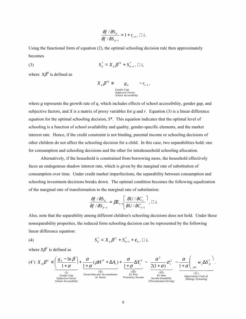
Using the functional form of equation (2), the optimal schooling decision rule then approximately

becomes

(3) *1

*−+= it

Nitit SXS β , ∀ i,

where XβN is defined as

1

−−≡ t

ityAccessibilSchoolFactorSubjective

GapGenderit

Nit rgX β ,

where g represents the growth rate of q, which includes effects of school accessibility, gender gap, and

subjective factors, and X is a matrix of proxy variables for g and r. Equation (3) is a linear difference

equation for the optimal schooling decision, S*. This equation indicates that the optimal level of

schooling is a function of school availability and quality, gender-specific elements, and the market

interest rate. Hence, if the credit constraint is not binding, parental income or schooling decisions of

other children do not affect the schooling decision for a child. In this case, two separabilities hold: one

for consumption and schooling decisions and the other for intrahousehold schooling allocation.

Alternatively, if the household is constrained from borrowing more, the household effectively

faces an endogenous shadow interest rate, which is given by the marginal rate of substitution of

consumption over time. Under credit market imperfections, the separability between consumption and

schooling investment decisions breaks down. The optimal condition becomes the following equalization

of the marginal rate of transformation to the marginal rate of substitution:

∂∂∂∂

=∂∂∂∂

−−

− 11

1 //

//

t

tt

it

it

CUCU

ESfSf β , ∀ =i.

Also, note that the separability among different children's schooling decisions does not hold. Under these

nonseparability properties, the reduced form schooling decision can be represented by the following

linear difference equation:

(4) ititC

itit SXS εβ ++= −*

1* , ∀ i,

where XβC is defined as

(4’)

SchoolingSiblingsofCostsyOpportunit

ijjtj

yInstabilitIncomeAnteEx

t

IncomeTransitoryPostEx

Tt

AssetsofonAccumulatiandOwnership

tP

ityAccessibilSchoolFactorSubjectiveGapGender

itCit SwYAHgX

'

)IV(

*

Saving)ary Precaution(

)III'(

22

)III(

)II(

)I(

1)1(21)(

11ln

∆

+−

+−∆

++∆+

++

+−

≡≠α

ασα

αα

αρα

αα

ββ .

9

Note that εit indicates a mean zero expectation error of parental income Yt. We allow a possibility of

serial correlation of this expectation error. In our estimation, we use various proxy variables for X, which

includes the following five components (equation 4’). First, X includes the gender indicator variable, the

school accessibility variable, and household-specific subjective factors of educational investments. The

second component of X is the ownership and accumulation of human and physical assets. The third term

(III) shows that an ex post realization of transitory income of parents, ∆YtT, has a positive impact on child

schooling. In contrast to a household with perfect credit availability, where parental income variable does

not affect child schooling, a credit-constrained household faces a high marginal cost of schooling if there

is a negative income shock. This reflects that consumption and schooling decisions are not separable

under a binding credit constraint. The fourth term (III’) shows the negative effect of income instability.

This term basically indicates that, given a positive third derivative of utility function, there is a motive for

precautionary saving as an ex ante optimal behavior against income instabilities. The positive

precautionary saving negatively affects child education since there is resource competition between asset

accumulation and investment in education. The final term indicates educational resource competition

among siblings. For example, an increase in other children's schooling time, ∆S*jt, ∀ j ≠ i, or its

opportunity cost, wj∆S*jt, decreases child i's optimal level of schooling.8 Alternatively, the wage earnings

of older siblings will enhance the optimal time allocation to schooling by decreasing wj∆S*jt.

Testable Restrictions

The important testable hypothesis can be derived by comparing equation (4) with equation (3). We can

easily note that the four terms of the right-hand side of equation (4)—terms (II), (III), (III’), and (V)—

should be 0 under perfect credit availability. On the other hand, under the binding credit constraint,

proxy variables for asset ownership and accumulation, transitory income, income stability, and sibling

variables should affect a child’s schooling behavior. Hence, our theoretical framework offers testable

restrictions that characterize two different credit regimes.

The economic intuition of these results should be clear. The two terms (II) and (III) in equation

(4’) indicate that a household’s overall resource constraint and life-cycle considerations will determine

the total amount of expenditure devoted to education. Credit and insurance availability become

==========================================================

8 According to equation (4), the optimization behavior of a household for the ith child is conditional on that for allother children. The optimal choice of child i’s schooling, S*i , depends on S*-i, the optimal schooling decision madefor a child other than i. We therefore derived a Nash equilibrium of child educational decisions implicitly. Strategiesthat comprise a Nash equilibrium at each date are referred to as Markov perfect. The equilibrium represented byequation (4) can thus be interpreted as the Markov perfect equilibrium (Maskin and Tirole 1988; Pakes and McGuire

10

especially important at this stage. If borrowing is allowed under an exogenously given interest rate, a

household can maximize the total wealth simply by investing in the human capital of each child so that

the marginal rate of return from educating each child is equal to the interest rate. However, if credit

availability is limited and thus household’s consumption and investment decisions are not separable, the

household resource availability such as parental income and assets affect the cut-off shadow interest rate

for educational investments. For example, when there is an unexpected income shock, credit-constrained

poor households have relatively high marginal utility of current consumption. This leads to an increase in

the cut-off shadow interest rate and a decrease in child education. In this case, implicit or explicit child

labor income can act as insurance that compensates for unexpected income shortfalls of parents.9

4 The Econometric Framework

There are two empirical approaches for investigating the schooling decision-making process, based on the

basic investment model of equation (4).10 First, the traditional approach employs a simple linear

regression model for years of schooling with various household background variables as explanatory

variables (Taubman 1989). However, the problem of this approach is that the linear regression model

combines the sequential schooling decision process into an estimation of time-invariant parameters and

therefore parameters in the model cannot be interpreted well as structural parameters.

The second approach formalized the process of schooling as a stochastic decision-making model

(Mare 1980; Lillard and Willis 1994, Behrman et. al., 2000). The model explicitly investigates the

determinants of sequence of grade transition probabilities. In other words, the probability of schooling at

τth grade conditional on completing schooling at τ-1th grade is empirically estimated. The model has a

substantial advantage over the linear regression approach since it gives estimates of structural parameters.

The statistical foundation of estimating such a sequential decision-making model was first provided by

Amemiya (1975). The model framework was then applied to estimation of schooling grade probabilities

===========================================================================================================================================================================================

1994; Besley and Case 1993).9 In fact, many estimates of schooling function using household data sets from developing countries report positivecoefficients of current household income variables, which imply the existence of credit market imperfections(Behrman and Knowles 1999; King and Lillard 1987; Sawada 1997).10 In fact, a third approach consists of applying the structural estimation framework for a dynamic stochastic discretechoice model. For a literature survey, see Amemiya (1996) and Eckstein and Wolpin (1989). Yet, given a householdhaving n children, the household’s schooling choice set is composed of 2n mutually exclusive, discrete dependentvariables. Since n takes about seven on average in our households from Pakistan, the structural estimation of such amodel will be computationally intractable. Applications of this framework to development issues include estimatesof the gender and age specific values of Korean children (Ahn 1995), an analysis of sequential farm labor decisionsusing Burkina Faso’s data (Fafchamps 1993), well investment decisions in India (Fafchamps and Pender 1997),bullock accumulation decisions of Indian farmers (Rosenzweig and Wolping 1993), and an analysis of fertility

11

with family background characteristics as determinants of these probabilities. For example, using a

Malaysian data set, Lillard and Willis (1994) estimated the sequential schooling decision model,

controlling for individual unobserved heterogeneity. Cameron and Heckman (1998) constructed an

alternative choice-theoretic model to examine how household background affects the school transition

probabilities. Other papers focus on only one transition out of the many sequences of schooling process,

such as the transition probability of high school graduates (Willis and Rosen 1979).

We will follow the second econometric approach and estimate the sequential schooling decision

model jointly. To estimate probabilities of the sequential decisions with an assumption of serial

correlation, we employ the full-information maximum likelihood method. Recall that there are the three

levels of education in Pakistan: primary, secondary, and postsecondary. Educational outcomes are

assumed to result from the five sequential decisions, as discussed in Section 2.

To formalize the sequential schooling process, we can define an indicator variable of schooling:

(5) δiτ = 1 if S*iτ > 0

= 0 otherwise,

where τ indicates the τth stage of education and S* is a latent variable and corresponds to the schooling

time variable, S*, in equation (4). Note that δiτ = 1 if child i goes to school at the τth stage of education.

We discretize the years of schooling into five categories, and thus τ takes on five values. With this new

discrete variable, the sequential process of schooling decision is described as follows: children are born

with zero years of schooling. If children become the age of six or so, some children enter primary school,

while other children stay uneducated. The uneducated children with no primary school entry, S*i1 = 0, is

represented by the indicator variable δi1 = 0. Having entered primary school (S*i1 > 0 and δi1 = 1), some

children finish primary school (δi2 = 1 or S*i2 > 0) while other children drop out from primary school (δi2

= 0 or S*i2 ≤ 0). Then, of those children who have finished primary school, some enter secondary school

(δi3 = 1 or S*i3 > 0), while others do not (δi3 = 0 or S*i3 ≤ 0). Given entered secondary school, some

children finish secondary school (δi4 = 1 or S*i4 > 0), while other children do not (δi4 = 0 or S*i4 ≤ 0).

Finally, after finishing secondary school, some children enter postsecondary school (δi5 = 1 or S*i5 > 0),

although others do not (δi5 = 0 or S*i5 ≤ 0).

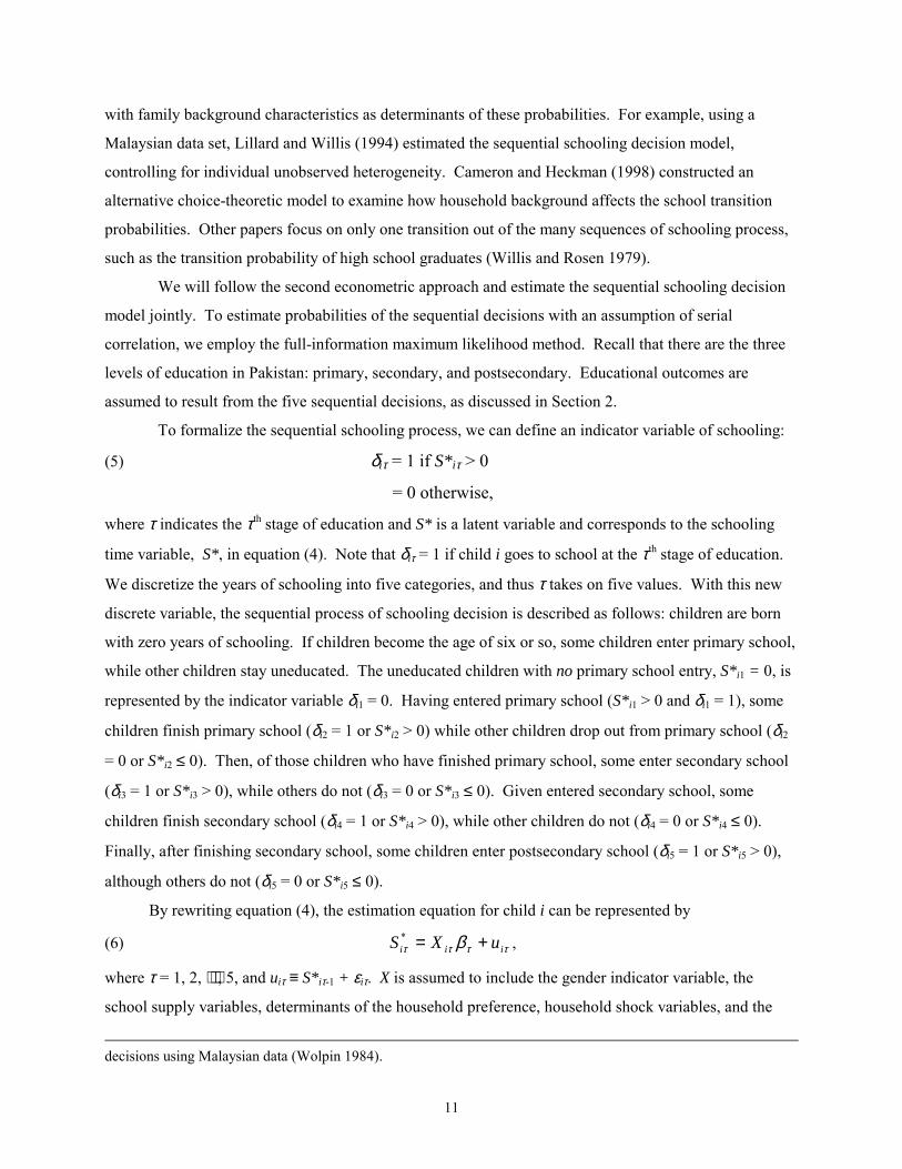
By rewriting equation (4), the estimation equation for child i can be represented by

(6) ττττ β iii uXS +=* ,

where τ = 1, 2, ⋅⋅⋅, 5, and uiτ ≡ S*iτ-1 + εiτ. X is assumed to include the gender indicator variable, the

school supply variables, determinants of the household preference, household shock variables, and the

===========================================================================================================================================================================================

decisions using Malaysian data (Wolpin 1984).

12

sibling composition variables. Note that S*i0 = 0 by construction.

Under an assumption that the decision making is independent across stages, or equivalently, uiτ is

independent across τ, the sequential model of equation (5) and (6) can be estimated by maximizing the

likelihood functions of dichotomous models repeatedly (independent error term specification) (Amemiya,

1975). However, our theoretical result indicates that schooling decisions are not independent across

stages by construction. It is straightforward to show that Cov(S*iτ, S*iτ-1) ≠ 0, since uiτ ≡ S*iτ-1 + εiτ.

These correlations can be explained, for example, by some unobserved propensity for schooling that is

stronger among the children who graduated from a certain grade than among the children who did not

finish this grade.

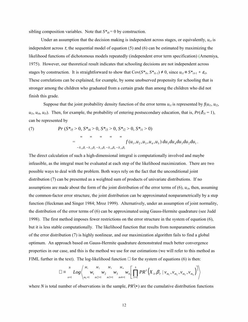
Suppose that the joint probability density function of the error terms uiτ is represented by f(ui1, ui2,

ui3, ui4, ui5). Then, for example, the probability of entering postsecondary education, that is, Pr(δ i5 = 1),

can be represented by

(7) Pr (S*i5 > 0, S*i4 > 0, S*i3 > 0, S*i2 > 0, S*i1 > 0)

= 1234554321 ),,,,(11 22 33 44 55

dududududuuuuuufi i i i iX X X X X

∞

−

∞

−

∞

−

∞

−

∞

−β β β β β

.

The direct calculation of such a high-dimensional integral is computationally involved and maybe

infeasible, as the integral must be evaluated at each step of the likelihood maximization. There are two

possible ways to deal with the problem. Both ways rely on the fact that the unconditional joint

distribution (7) can be presented as a weighted sum of products of univariate distributions. If no

assumptions are made about the form of the joint distribution of the error terms of (6), uiτ, then, assuming

the common-factor error structure, the joint distribution can be approximated nonparametrically by a step

function (Heckman and Singer 1984; Mroz 1999). Alternatively, under an assumption of joint normality,

the distribution of the error terms of (6) can be approximated using Gauss-Hermite quadrature (see Judd

1998). The first method imposes fewer restrictions on the error structure in the system of equation (6),

but it is less stable computationally. The likelihood function that results from nonparametric estimation

of the error distribution (7) is highly nonlinear, and our maximization algorithm fails to find a global

optimum. An approach based on Gauss-Hermite quadrature demonstrated much better convergence

properties in our case, and this is the method we use for our estimations (we will refer to this method as

FIML further in the text). The log-likelihood function ℑ for the system of equations (6) is then:

( )∏= = = = ==

=ℑN

n

M

m

M

m

M

mmmmmi

M

mvvvvXPRwwwwLog

1 1 12 14

5

14

13321

1

1

2 4

4321

3

,,,|τ

τττ β

where N is total number of observations in the sample, PRτ(• ) are the cumulative distribution functions

13

for every equation in system (6) conditional on the common factors, v’s and w’s are one-dimentional

quadrature points (nodes) and weights from a Gauss-Hermite rule (Stroud and Secrest 1966), M’s are the

numbers of quadrature points. As before, X’s represent the equation specific sets of explanatory variables

and β’s are the vectors of unknown parameters to be estimated.

The estimations presented in the paper are based on the approximation of the probability integral

by Gauss-Hermite quadrature with four nodes.11 Further increase in the number of nodes fails to improve

the value of log-likelihood function. Identification is achieved through inclusion of the set of stage-

specific variables such as school supply variables, household human and physical assets, and household

income and health shock variables, as will be discussed in the next subsection. According to the

likelihood-ratio test criterion, the independent error specification is rejected in favor of the FIML

specification that assumes a joint normality of the error distribution.12

5.1 Variables

As we estimate the above sequential schooling model, we start by inspecting the basic data

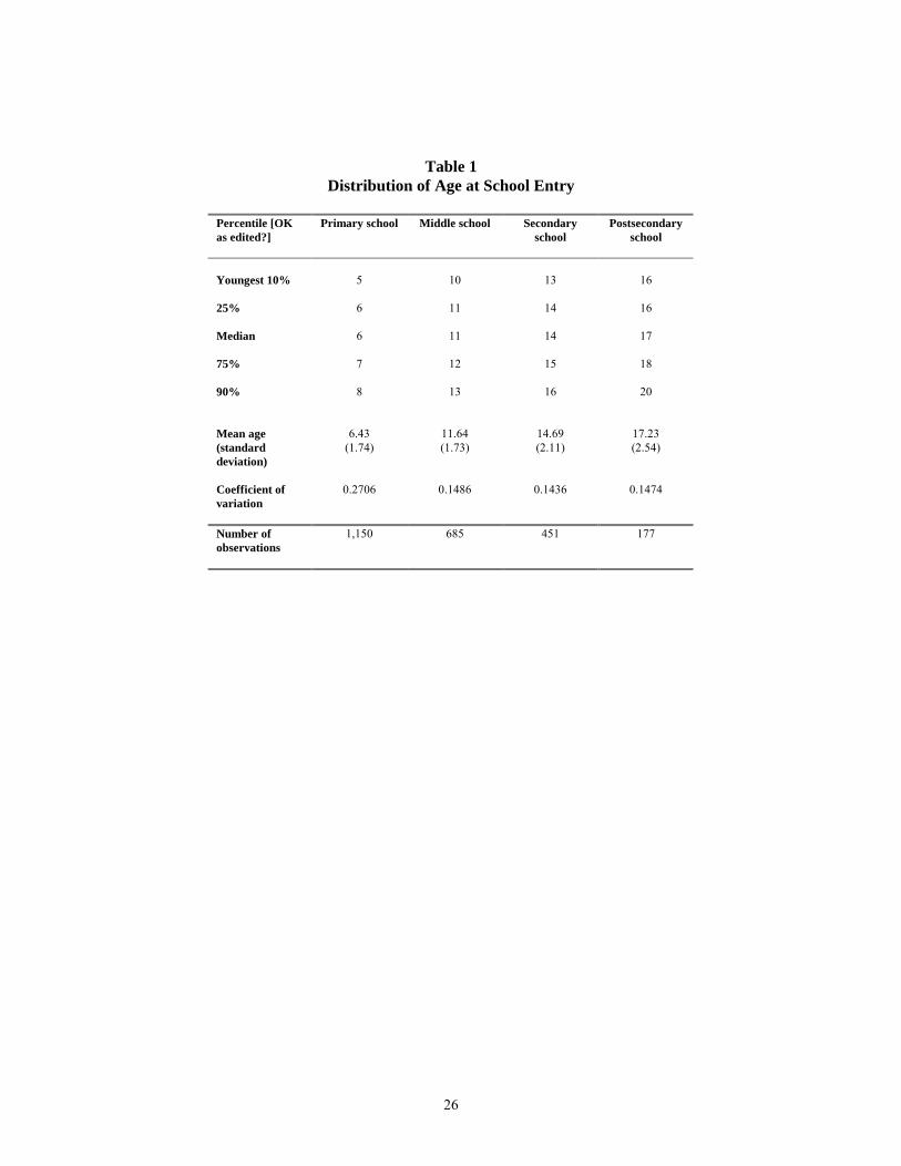
characteristics. According to the median age of school entry, children enter primary schools at the age of

six, secondary schools at the age of eleven, and postsecondary schools at the age of seventeen (Table 1).

Moreover, our survey data show that primary and secondary education last an average of five and six

years, respectively. Since the formal length of the secondary-level schooling is five years in Pakistan, an

extra year in secondary education in our sample indicates that grade repetition or a delay of secondary

school entry, which is quite common in Pakistani villages.

Table 3 summarizes descriptive statistics of variables used in the sequential model of equation (6)

as the discrete dependent variable, S*iτ, and covariates of conditional probabilities, X. According to our

theoretical model (4), X is assumed to include gender gap indicator variables, school supply variables,

subjective discount factor, physical and human assets, transitory income change, and sibling composition

variables.

The gender gap indicator variables are divided into two subgroups according to province. The

first gender variable is for Punjab province and is a dummy variable taking 1 for females in Punjab

==========================================================

11 Parameters of the model are estimated by maximum likelihood using DFP algorithm (Powell 1977) with analyticalderivatives. The variance-covariance matrix of the estimated coefficients is estimated by approximating theasymptotic covariance matrix by the so-called “sandwich” estimator (see, for example, Davidson and MacKinnon1993, 263).12 Results of the independent error term specification are available from authors upon request. While the independenterror term model is thought to provide biased coefficients owing to correlations of sequential decisions, qualitativeresults of the independent error model and the FIML estimates are comparable.

14

province and 0 otherwise. Similarly, the second gender dummy variable for NWFP takes 1 for females in

NWFP and 0 otherwise. These female dummy variables indicate that the share of female students

declined at the primary school entry level (Table 3).

The second block of independent variables contains the gender-specific school supply variables.

The first supply variable takes 1 only if the child is male and there is a male school within the village of

the child’s residence. Otherwise, this variable takes 0. The second supply dummy variable takes 1 only if

the child is female and there is a female school within the village. We can see that for primary school

entry level, 37 percent of male children do not face supply constraints, whereas only 18 percent of girls

have access to female schools in their village (Table 3).13

Third, we assume that a household’s subjective preference depends on the household’s social

class or caste status. Traditionally, the caste status, called biraderi in Punjab and quom in NWFP, is

identified with an occupational position (Eglar 1960; Ahmad 1977; Barth 1981; Ahmed 1980). For

example, agricultural landless laborers are strictly distinguished from landowners. Nonagricultural

laborers such as casual laborers and artisans are also differentiated from landowners. This system of

caste has prevailed in the form of social norms, and members of each class are expected to act according

to their social and economic status. Hence, the caste system indirectly constrains the educational

opportunities of low-caste children. In order to capture these sociocultural effects, we include parents’

occupation dummy variables—farmers with land, landless farmers or nonfarm casual laborers, and

business and government officials. The default variable is those who are unemployed and/or at home

because of sickness or unemployment. According to Table 3, more than 30 percent of our sample is

composed of farmers with land for all schooling processes. It is notable that, at higher schooling stages,

the fraction of children from landless farmers or casual laborers declines significantly. On the other hand,

the share of children of farmers with land ownership increases after secondary school entry. These casual

findings are consistent with the sociocultural background of Pakistani society.

The fourth set of variables is composed of household human and physical asset variables.14 The

first two variables are time-invariant dummy variables for father and mother’s education, which take 1 if

the father or mother has completed at least primary school and take 0 otherwise. Household physical

asset variables include the amount of land ownership and a dummy variable for tractor ownership. We

can easily see that all four of these household asset variables increase as the child education level

increases (Table 3). Children who are studying at higher levels of education are basically from relatively

==========================================================

13 No village in our sample has upper-secondary and/or postsecondary education. This implies that supply constraintssuch as the accessibility of schools are severe at higher levels of education.14 Although our theory requires us to include asset accumulation as independent variables, we utilize a total assetvariable instead of its first difference. This is simply because markets for land and agricultural machinery are thin in

15

rich households of educated parents.

With respect to the transitory income shock variables, the model includes good- or bad-year

dummy variables based on household’s subjective and retrospective assessment of agricultural

production, wage earnings, and livestock income. The health shock effects are also considered by

including dummy variables for the health of the household head and the wife, which take 1 if they are

physically inactive and take 0 otherwise. As Jacoby and Skoufias (1997) pointed out, a distinction

between unanticipated and anticipated components of transitory income movements might be important.

The health shocks might be interpreted as the unanticipated components since these shocks are largely

unexpected. On the other hand, income movements include both anticipated and unanticipated

components.

As sibling variables, we take the number of older brothers and sisters. Alternatively, we can

incorporate more detailed sibling composition variables, separated by current schooling status. Yet, our

older sibling variables are predetermined, and thus we may be allowed to regard these variables as being

exogenous. The descriptive statistics show that there is a negative relationship between education level

and the number of older brothers and sisters (Table 3). This finding suggests that those students who

could obtain higher education are from households with a small number of children. This can be a

reflection of intrahousehold resource competition or birth-order effect.

Finally, according to the age distribution of sampled children of the household head, the average

age of children is 20.5 in 1998. However, there is a large variation in age. Some members are older than

50. The age distribution indicates that there will be a potentially large cohort effect, and thus the

empirical model needs to control for it. Hence, we include age cohort dummy variables.

5.2 Estimation Results of the Sequential Schooling Decision Model

Columns in Table 5 summarize a set of estimated coefficients of the full sequential schooling decision

model for each school level. These results are a derived FIML estimation of conditional probabilities

represented by equations (7) and (8). Detailed descriptions and interpretations of our FIML estimation

results are presented below.

Gender Gap

First, coefficients on gender dummy variables indicate that daughters have lower conditional schooling

===========================================================================================================================================================================================

rural Pakistan and thus we do not observe change in assets frequently.

16

probabilities at the primary entry and exit levels than sons have. The female coefficients in Punjab

province are smaller than those in NWFP at the primary school entry, indicating a smaller gender gap in

Punjab. This regional difference seems to be largely due to the different degree of sociocultural

constraints. Yet the coefficients on the female dummy variable are not statistically significant after

secondary school entry. The gender gap in education seems to disappear among the students who are

studying at secondary and postsecondary level schools. Therefore, schooling progression rates become

comparable between male and female students at higher levels of education. Table 6 summarizes the

discrete marginal change of schooling probabilities with respect to gender dummy variables, evaluated at

mean dependent variables.15 We can easily verify that the marginal effects are different between girls and

boys at the primary school entry level, while the difference disappears at the secondary school exit level.

These marginal effects confirm the above interpretation of the estimation results in Table 5.

Development researchers and practitioners have argued that women are significantly less

educated than men in Pakistan (Khan 1993; Shah 1986; Chaudhary and Chaudhary 1989; Behrman and

Schnieder 1993). There are several possible explanations for the distinct gender gap in education. For

example, the high opportunity costs of daughters’ education in rural Pakistan may lead to apparent

intrahousehold discrimination against women in terms of education. Because of the custom of seclusion

of women, purdah, parents might have a strongly negative perception of female education. However, our

estimation results represent that evidence is not so simple or monotonic. Although there is a distinct

gender gap in primary-level education, the gap is likely to disappear among those who have entered

secondary education.

School Supply

The school availability coefficients are positive and significant for female schools, while the coefficient is

not statistically significant for male schools. This result suggests that the lack of primary and secondary

schools in the village clearly impedes female education, while supply-side constraints are not severe for

male students. The marginal effect of primary school availability within the village is represented in

Table 7.16 According to Table 7, accessibility to a primary school within the village seems to contribute

==========================================================

15 To calculate the marginal effects in a given simulation, the certain value of the variable of interest is assigned to allthe households in the sample in a particular state. The simulated probabilities are generated for each household byintegrating over the estimated distribution and averaging the probabilities across the sample. Next, the value of thevariable of interest is changed, and this changed value is assigned to the whole sample of the households. Then thenew set of simulated probabilities is generated. The marginal effect—that is, the effect of the changes in the particularparameter on the probabilities of school participation—is calculated as a difference in these simulated probabilities.16 See footnote 15 for explanations of our methodology to calculate the marginal effects.

17

to a 18 percent increase in a girl’s primary school entry probability. Moreover, female primary school

drop out will decline by 16%. In fact, our qualitative survey data show that, in 32.5 percent of school

termination decisions, households listed the supply side as the main reason for their decision problems,

including inaccessibility to school and the low teacher quality (Table 4). A significant portion of the

gender gap in Pakistani education may be explained by supply-side quantity and quality constraints

(Alderman et al. 1995, 1996). Although traditional Pakistani culture requires single-sex schools, the lack

of school availability affects female education more seriously than male education (Shah 1986). Parents

are unwilling to send daughters to school if a female school is not available nearby. Since allowing girls

to cross a major road or a river on the way to school often involves the risk that daughters will break

purdah, parents will choose not to let daughters go to school. Moreover, sociocultural forces also create

the needs for women teachers to teach female students in the village. It has been pointed that irrespective

of the monetary or nonmonetary incentives in the form of scholarships, girls will come only if schools are

opened with female teachers in each village (Chaudhary and Chaudhary 1989).17 Even if a girl’s school is

available in the village, a chronic shortage of women teachers imposes serious constraints on female

education.

Social Class Effects

The overall estimated coefficients of the social class variable indicate that, at primary and postsecondary

entry levels, children of business or government official households have the highest schooling

probability among the social classes considered. The second finding is that the farmers with land

ownership have higher level of educational investments at the primary school entry level than landless

farmers or casual labor households. These results suggest that the occupation, which is traditionally

related to social status, affects educational investment decisions at the initial entry decision to schools and

at higher levels of education.

==========================================================

17 Although the supply of teachers is constrained in part by the shortage of women candidates, the villageenvironment also prevents expansion of female teachers in rural areas. Attracting and retaining high-quality femaleteachers from outside villages poses a different set of problems, since they must relocate, gain local acceptance, andclear the difficult hurdle of finding suitable accommodations. Even locally recruited teachers could be chronicallyabsent from school because of responsibilities for their household chores (Khan 1993). Nevertheless, there is notenough monetary compensation to attract women to be teachers. Provincial governments, for instance, provideteachers in villages with lower allowances for house rent than teachers in urban areas. Moreover, there might be a

18

Parental Human Assets

Father and mother’s education variables have consistently positive and significant coefficients in all

levels of schooling except at the secondary school exit level. These estimation results indicate important

complementarity between the education of the parents and the child schooling investments. This

complementarity is generated possibly by educated parents’ positive incentive of educating children,

improved technical or allocative efficiency, and/or superior home teaching environments, as pointed out

by the preceding studies (Schultz 1964; Welch 1970; Behrman and others 2000). Subjective factors

might be important as well. According Table 4, in 13.4 percent of cases, households listed “the

accomplishment of the desired education level” as the primary reason of a child’s school dropout. This is

a purely subjective reason, implying that schooling choice may differ depending on ethnicity, network,

and social status (Psacharopoulos and Woodhall 1985). The more educated mother and father seem to be

better able to perceive the benefit of education than uneducated parents, since they can estimate returns to

education more precisely.

Household Physical Assets

At the primary school entry decision, while the tractor ownership variable has a positive and significant

coefficient, land ownership has a negative significant coefficient. This asymmetry in two physical assets

might be attributable to the difference in complementarity with education. In poor Pakistani villages,

tractor ownership is an obvious measure of a household’s wealth. Hence, our results suggest that the

primary school entry probability of children is systematically higher for households with wealth.

Moreover, it has been argued that technology and education have complementarity (Psacharopoulos and

Woodhall 1985; Foster and Rosenzweig 1996). It is likely that tractor operation requires at least a basic

level of education. On the other hand, the negative coefficient of land ownership at the primary school

entry level might suggest that there is a complementarity between land ownership and on-farm child

work, which results in less education of children.

At the postsecondary education entry level, both tractor and land ownership have positive and

statistically significant coefficients on the conditional schooling probability. At this level, household

ownership of physical assets seems to play an important role in education decisions. In general,

households’ resource availability extends their self-insurance ability and thus encourages high-risk and

high-return investment opportunities. Risk-taking and precautionary saving behaviors may be closely

===========================================================================================================================================================================================

school quality problem originating from the teacher’s low level of education (Warwick and Jatoi 1994).

19

related to physical asset ownership (Morduch 1990). The negative effect of accumulating precautionary

saving on educational investment will be less severe for those households that have assets.

Household Shock Variables

Negative income shocks discourage schooling continuation significantly at the primary school exit and

the secondary school entry and exit levels. Moreover, negative health shocks increase dropouts from

secondary school. These estimation results are favorable to our theoretical model under binding credit

constraints (Equation 4). In general, Pakistani households face considerable income instabilities. Risks

of disaster such as large income shortfalls, sickness, and sudden death of an adult member impose serious

constraints on a household’s resources, since there is a severe limitation on formal and/or informal

insurance and credit availability in rural areas. Accordingly, exogenous negative shocks have non-

negligible effects on the household’s educational investment decisions. Pakistani households might adopt

perverse informal self-insurance devices by using child labor income as parental income insurance,

sacrificing the accumulation of human capital.18

Sibling Competition

According to the estimated coefficients in the sibling variables block, the number of older sisters seems to

be associated with more primary education for younger siblings. This finding is consistent with

Greenhalgh (1985) and Parish and Willis (1993) using Taiwanese data. Older sisters may extend the

household’s resource availability, either by marrying early or by providing domestic labor. This suggests

that households are not discriminating against all daughters, although the older daughters might bear a

large portion of burden under binding resource constraints (Strauss and Thomas 1995).

On the other hand, at the secondary school exit and postsecondary entry levels, the number of

older brothers, instead of the number of older sisters, increases schooling probabilities. These results

suggest that once a child is picked as a “winner” of educational investment within the family, his or her

education at the secondary and postsecondary level is supported partly by the older brother’s resource

contributions. At these higher levels of education, an older brother’s farm or nonfarm monetary income

contributions to household resources might be more important and significant than a daughter’s

nonmarket domestic labor contribution to the household.

==========================================================

18 Sawada (1997) and Alderman et. al. (2000) also found the important impact of shocks on school enrollments inrural Pakistan.

20

Existing empirical studies indicate mixed results for birth-order effects—that is, the sibling

resource competition effects over time.19 There is no consensus in the literature about whether birth-order

effects really exist, and if they exist, whether they are positive, negative, or nonlinear in form (Parish and

Willis 1993). Our estimation results suggest that, under credit constraints, birth-order effects exist, and,

more important, the effects are specific to gender and education level.

6 Concluding Remarks

This paper investigated the sequential educational investment process of Pakistani households by

integrating observations from the field, economic theory, and econometric analysis. The paper makes two

contributions to the literature. First, we use the unique data set on the whole retrospective history of child

education and household background, which was collected exclusively for this analysis through field

surveys in rural Pakistan. Second, in addition to the data contribution, this paper employed full-

information maximum likelihood method to cope with the complicated estimation procedure of multiple

integration of conditional schooling probability. This method, combined with the unique data set,

enabled us to estimate the full sequential model of schooling decisions.

The most striking feature revealed by the data is the high educational retention rate, conditional

on school entry. Moreover, we found important dynamics of the gender gap in education, the significance

of shock variables, wealth effects, and intrahousehold resource allocation with our full sequential

schooling model. These findings are consistent with a household’s optimal education investment under a

binding credit constraint.

Although the demand for education cannot be controlled directly by the government, supply-side

interventions will be effective. Our estimation results suggest that, in addition to household demand

considerations, raising the quantity of female primary schools has a substantial effect in improving

==========================================================

19 There are two possible cases (Behrman and Taubman 1986). The first possibility is a negative birth-order effect.As more children are born, the household resources constraint becomes severe and fewer resources are available perchild. If this per child resource shrinkage effect is dominant, the younger (higher-order) siblings will receive lesseducation than older siblings. Alternatively, the resource competition effects might decline over time, sincehouseholds can accumulate assets and increase income over time. Moreover, the older children may enter the labormarket, contributing to household resources. Therefore younger (higher-order) siblings could spend more years atschool. This is the case of positive birth-order effects. Also, an economy of scale due to household-level publicgoods might exist, since siblings can share various educational inputs and materials. Positive knowledge externalitiesmight be important as well, since younger children can learn easily from the experience of their older siblings throughhome teaching. In sum, having older siblings might promote the education of a younger child, rather than impede theeducation of that child, if the resource extension effects, scale economies, and externalities are larger than thecompetition effects.

21

education in Pakistan. Indeed, the push to expand access to schooling by increasing the supply of schools

has dominated the agenda for education in developing countries since the 1960s (Lockeed et al. 1991).

Yet remote and inappropriate female school locations and resultant high schooling costs are still serious

problems in rural Pakistan. Hence, the cost-effectiveness of providing primary education can be

significantly improved, if the allocation of funds is shifted toward recurring expenditures for construction

of female schools and employment of more female teachers. These supply-side policy interventions have

significant potential for reducing gender biases in human capital investment. We should also note that

closing the gender difference in education creates long-lasting positive effects on economic development,

since education of mothers relates to fertility and population over time. Many empirical studies show a

highly educated mother has lower infant mortality rate, fewer children, and more educated and healthier

children (King and Hill 1993).

22

References

Ahmad, S. 1977. Class and Power in a Punjabi Village (NY: Monthly Review Press).Ahmed, A. S. 1980. Pukhtun Economy and Society: Traditional Structure and Economic

Development in a Tribal Society (London: Routledge & Kegan Paul).Ahn, N. 1995. “Measuring the Value of Children by Sex and Age Using a Dynamic Programming

Model.” Review of Economic Studies 62 (3), July: 361-79.Alderman, H. 1996. “Saving and Economic Shocks in Rural Pakistan,” Journal of Development

Economics 51 (2), December: 343-65.Alderman, H., J. Behrman, S. Khan, D. R. Ross, and R. Sabot. 1995. “Public Schooling Expenditures

in Rural Pakistan: Efficiently Targeting Girls and a Lagging Region.” In D. van de Walle andK. Mead, eds., Public Spending and the Poor: Theory and Evidence (Washington, D.C.: WorldBank).

Alderman, H., J. Behrman, V. Lavy, and Rekha Menon, 2000, “Child Health and School Enrollment: ALongitudinal Analysis,” forthcoming, Journal of Human Resources.

Alderman, H., J. Behrman, D. Ross, and R. Sabot, 1996. “Decomposing the Gender Gap in CognitiveSkills

in a Poor Rural Economy,” Journal of Human Resources 31 (1), 229-54.Alderman, H., and M. Garcia. 1993. Poverty, Household Food Security, and Nutrition in Rural

Pakistan. IFPRI Research Report 96 (Washington, D.C.: International Food Policy ResearchInstitute).

Alderman, H., and P. Gertler. 1997. “Family Resources and Gender Difference in Human CapitalInvestments: The Demand for Children’s Medical Care in Pakistan.” In L. Haddad, J.Hoddinott, and H. Alderman eds., Intrahousehold Resource Allocation in DevelopingCountries: Models, Methods, and Policy (Baltimore: Johns Hopkins University Press).

Amemiya, T. 1975. “Qualitative Response Models.” Annals of Economic and Social Measurement4 (3), Summer: 363-72.

———. 1996. “Structural Duration Models.” Journal of Statistical Planning and Inference 49:39-52.

Barro, R. J., and X. Sala-i-Martin. 1995. Economic Growth (New York: McGraw-Hill).Barth, F. 1981. Features of Person and Society in Swat: Collected Essays on Pathans (London:

Routledge & Kegan Paul).Behrman, J. R., A. D. Foster, M. R. Rosenzweig, and P. Vashishta. 2000. “Women’s Schooling,

Home Teaching, and Economic Growth.” Journal of Political Economy 107 (4): 682-714.Behrman, J. R. and J. C. Knowles. 1999. “Household Income and Child Schooling in Vietnam” World

Bank Economic Review 13 (2): December, 211-56.Behrman, J. R., and R. Schneider. 1993. “An International Perspective on Pakistani Human Capital

Investments in the Last Quarter Century.” Pakistan Development Review 32 (1), Spring: 1-68.Behrman, J. R., P. Sengupta, and P. Todd, 2000, “Progressing through PROGRESA: An Impact

Assessment of Mexico’s School Subsidy Experiment,” processed, International Food PolicyResearch Institute.

Behrman, J. R., and P. Taubman. 1986. “Birth Order, Schooling, and Earnings.” Journal of LaborEconomics 4 (3), July: S121-S145.

Besley, T., and A. Case. 1993. “Modelling Technology Adoption in Developing Countries.”AEA Papers and Proceedings 83 (2), May: 396-402.

Birdsall, N. 1991. “Birth Order Effects and Time Allocation.” In T. P. Schultz, ed. Research inPopulation Economics, Vol. 7 (Greenwich, Conn.: JAI Press).

Cameron, S. V., and J. Heckman. 1998. “Life Cycle Schooling and Dynamic Selection Bias: Modelsand Evidence for Five Cohorts of American Males.” Journal of Political Economy 106 (2), April:

23

262-333.Chaudhary, N. P., and A. Chaudhary. 1989. “Incentives for Rural Female Students in

Pakistan.” BRIDGES project, Harvard Institute of International Development and thethe Academy of Educational Planning and Management, Pakistani Ministry of Education.Mimeo (Islamabad, Pakistan).

Davidson, R., and J. G. MacKinnon. 1993. Estimation and Inference in Econometrics (New York: OxfordUniversity Press).

Eckstein, Z., and K. I. Wolpin. 1989. “The Specification and Estimation of Dynamic StochasticDiscrete Choice Models.” Journal of Human Resources 24 (4), Fall: 562-98.

Eglar, Z. 1960. A Punjabi Village in Pakistan (New York: Columbia University Press).Fafchamps, M. 1993. “Sequential Labor Decisions under Uncertainty: An Estimable Household

Model of West-African Farmers.” Econometrica 61 (5), September: 1173-97.Fafchamps, M., and J. Pender. 1997. “Precautionary Saving, Credit Constraints, and

Irreversible Investment: Theory and Evidence from Semi-Arid India.” Journal of Businessand Economic Statistics 15 (2), April: 180-94.

Fafchamps, M., and A. R. Quisumbing. 1999. Human Capital, Productivity, and Labor Allocation inRural Pakistan. Journal of Human Resources 34 (2), Spring: 369-406.

Foster, A., and M. R. Rosenzweig. 1996. “Technological Change and Human-Capital Returns andInvestments: Evidence from the Green Revolution.” American Economic Review 86 (4),September: 931-53.

Garg, A., and J. Morduch. 1998. “Sibling Rivalry and the Gender Gap: Evidence from Child HealthOutcomes in Ghana.” Journal of Population Economics 11 (4), December: 471-93.

Greenhalgh, S. 1985. “Sexual Stratification in East Asia: The Other Side of ‘Growth with Equity’in East Asia.” Population and Development Review 11 (2), June: 265-314.

Heckman, J., and E. Singer. 1984. “A Method of Minimizing the Impact of Distributional Assumptions inEconometric Models for Duration Data.” Econometrica 52 (2), March: 271-320.

Ismail, Z. H. 1996. “Gender Differentials in the Cost of Primary Education: A Study ofPakistan.” Pakistan Development Review 35 (4): 835-49.

Jacoby, H., and E. Skoufias. 1997. “Risk, Financial Markets and Human Capital in a DevelopingCountry.” Review of Economic Studies 64 (3), July: 311-35.

Judd, K. L. 1998. Numerical Methods in Economics (Cambridge, Mass.: MIT Press).Khan, S. R. 1993. “Women's Education in Developing Countries: South Asia.” In E. M. King and

Anne M. Hill, eds., Women's Education in Developing Countries: Barriers,Benefits, and Policies (Baltimore: Johns Hopkins University Press for theWorld Bank).

King, E. M., and A. M. Hill, eds. 1993. Women’s Education in Developing Countries (Baltimore: JohnsHopkins University Press for World Bank).

King, E. M., and L. Lillard. 1987. “Education Policy and Schooling Attainment in Malaysia and thePhillipines.” Economics of Education Review 6 (2): 167-81.

Levhari, D., and Y. Weiss. 1974. “The Effect of Risk on the Investment in Human Capital.” AmericanEconomic Review 64 (6), December: 950-63.

Lillard, L. A., and R. J. Willis. 1994. “Intergenerational Educational Mobility: Effects of Family andState in Malaysia.” Journal of Human Resources 24 (4), Fall: 1126-66.

Lockheed, M. E., A. M. Verspoor, and associates. 1991. Improving Primary Education inDeveloping Countries (Washington, D.C.: World Bank).

Mare, R. D. 1980. “Social Background and School Continuation Decisions.” Journal of theAmerican Statistical Association 75 (370), June: 295-305.

Maskin, E., and J. Tirole. 1988. “A Theory of Dynamic Oligopoly I: Overview and QuantityCompetition with Large Fixed Costs.” Econometrica 56 (3), May: 549-69.

Morduch, J. 1990, “Risk, Production, and Saving,” draft, Harvard University.

24

Mroz, T. 1999. “Discrete Factor Approximations in Simultaneous Equation Models: Estimating theImpact of a Dummy Endogenous Variable on a Continuous Outcome.” Journal of Econometrics92 (2), October: 233-74.

Pakes, A., and P. McGuire. 1994. “Computing Markov-perfect Nash Equilibria: NumericalImplications of a Dynamic Differentiated Product Model.” Rand Journal of Economics 25 (4),Winter: 555-89.

Parish, W. L., and R. J. Willis. 1993. “Daughters, Education and Family Budgets: TaiwanExperiences.” Journal of Human Resources 28 (4), Fall: 868-98.

Powell, M. J. D. 1977. “Restart Procedures for the Conjugate Gradient Method.” MathematicalProgramming 12: 241-54.

Psacharopoulos, G., and M. Woodhall. 1985. Education for Development: An Analysis ofInvestment Choices (Washington, D.C.: World Bank).

Rosenzweig, M. R., and K. I. Wolpin. 1993. “Credit Constraints, Consumption Smoothing, andthe Accumulation of Durable Production Assets in Low-Income Countries: Investments inBullocks in India.” Journal of Political Economy 101 (2), April: 223-44.

Sawada, Y. 1997. Human Capital Investments in Pakistan: Implications of Micro Evidence fromRural Households.” Pakistan Development Review 36 (4), Winter: 695-712.

———. 1999. “Essays on Schooling and Economic Development: A Micro-econometric Approachfor Rural Pakistan and El Salvador.” Ph.D. diss., Stanford University, Department of Economics.

Schultz, T. W. 1964. Economic Value of Education (New York: Columbia University Press).Shah, N. M. 1986. Pakistani Women: A Socioeconomic and Demographic Profile (Islamabad, Pakistan:

Pakistan Institute of Development Economics; Honolulu, Hawaii: East-West Population Instituteof East-West Center.

Strauss, J., and D. Thomas. 1995. “Human Resources: Empirical Modeling of Household andFamily Decisions.” In J. Bherman and T. N. Srinivasan, eds., Handbook of DevelopmentEconomics, Vol. 3A (North-Holland: Elsevier Science Ltd.).

Stroud, A., and D. Secrest. 1966. Gaussian Quadrature Formulas (Englewood Cliffs, N.J.: Prentice Hall).Taubman, P. 1989. “Role of Parental Income in Educational Attainment.” AEA Papers and

Proceedings 79 (2), May: 57-61.Townsend, R. M. 1995. “Financial Systems in Northern Thai Villages.” Quarterly Journal of

Economics 110 (4), November: 1011-46.Warwick, D. P., and H. Jatoi. 1994. “Teacher Gender and Student Achievement in Pakistan.”

Comparative Education Review 38 (3): 377-99.Welch, F. 1970. “Education in Production.” Journal of Political Economy 78 (1) Jan-Feb: 35-59.Willis, R. J., and S. Rosen. 1979. “Education and Self-Selection.” Journal of Political Economy 87

(5), October: S7-S36.Wolpin, K. I. 1984. “An Estimable Dynamic Stochastic Model of Fertility and Child Mortality.”

Journal of Political Economy 92 (5), October: 852-74.Zeldes, S. P. 1989. “Consumption and Liquidity Constraints: An Empirical Investigation.” Journal of

Political Economy 97 (2), April: 305-46.

25

Appendix: A Summary of the Field Survey

Field surveys were conducted twice to gather information exclusively for this paper. In the first round ofthe survey in February through April 1997, the survey team carried out interviews in fourteen villages ofthe Fisalabad and Attock districts of Punjab province (Sawada, 1999). The selection of our survey siteswas predetermined, since we basically resurveyed the panel households that had previously beeninterviewed by the International Food Policy Research Institute (IFPRI) through the Food SecurityManagement Project, based on a stratified random sampling scheme (Alderman and Garcia 1993). Thefirst district in our sample, Faisalabad, is a well-developed irrigated wheat and livestock production area.The second district, Attock, is a rainfed wheat production region near the industrial city of Taxila. In thisdistrict earnings from nonfarm activities are the major component of household income. Then the secondround surveys were carried out in eleven villages of the Dir district of the North-West Frontier Province(NWFP) in December 1997 through January 1998. Dir is also a rainfed wheat production area with somecash crop production such as citrus. There is a limited set of nonfarm income-earning opportunitieswithin and around the district. However, temporary emigration to the Persian Gulf countries is commonin Dir. As a result, nonfarm income and remittances account for more than 60 percent of averagehousehold income, according to the IFPRI data files (Sawada 1999).

In our retrospective surveys, we used three different sets of questionnaires. The firstquestionnaire is composed of questions on basic child information and retrospective schooling progress.The second questionnaire collects basic household background information, such as household size,permanent components of household resources, and fluctuations in household assets and income overtime. With the third questionnaire, village-level retrospective information was gathered by interviewinglocal government officials and/or educated village dwellers such as schoolteachers. In particular, wecollected information about the year when male and female primary schools were built in the village.

These questionnaires seemed to work well in the field. Farmers remembered incidents related tochild education and enjoyed talking about their children. Each household interview lasted approximatelyone and a half to two hours, largely depending on the number of children. We visited the villages withoutprior notification, and the availability of respondents was uncertain in advance. Therefore, we mayplausibly assume that our attrition of panel households is determined by a random process.

Our field surveys covered 203 households in Punjab and 164 households in NWFP. Hence, 367households were interviewed, and information on a total of 2,365 children was collected. The combineddata set gives a complete set of retrospective histories of child schooling, together with household- andvillage-level information, which make the estimation of a full sequential schooling decision modelfeasible. Moreover, the field survey data set is matched with the IFPRI data files. Since our purpose is anestimation of the full sequential schooling decision model, we use part of the IFPRI data files thatcontains long-term retrospective information on household and village characteristics.

26

Table 1Distribution of Age at School Entry

Percentile [OKas edited?]

Primary school Middle school Secondaryschool

Postsecondaryschool

Youngest 10% 5 10 13 16

25% 6 11 14 16

Median 6 11 14 17

75% 7 12 15 18

90% 8 13 16 20

Mean age(standarddeviation)

6.43(1.74)

11.64(1.73)

14.69(2.11)

17.23(2.54)

Coefficient ofvariation

0.2706 0.1486 0.1436 0.1474

Number ofobservations

1,150 685 451 177

27

Table 2Sample Probability of School Continuation

Total Faisalabad Attock Dir

Male Female Male Female Male Female Male Female

Primary schoolentry

h1/n1 0.64 0.24 0.65 0.33 0.69 0.34 0.62 0.17

Primary schoolgraduate

h2/n2 0.82 0.69 0.74 0.72 0.87 0.69 0.84 0.67

Secondary schoolentry

h3/n3 0.93 0.53 0.97 0.34 0.89 0.59 0.94 0.64

Secondary schoolgraduate

h4/n4 0.59 0.71 0.47 0.87 0.53 0.75 0.68 0.62

Postsecondaryschool entry

h5/n5 0.57 0.57 0.55 0.77 0.39 0.56 0.64 0.48

Total number insample

n1 978 872 232 185 221 176 525 511

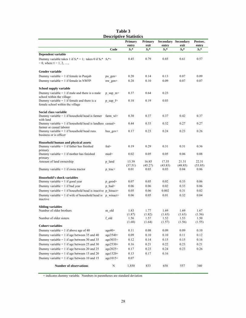
28

Table 3Descriptive Statistics

Primaryentry

Primaryexit

Secondaryentry

Secondaryexit

Postsec.entry

Code S1* S2* S3* S4* S5*Dependent variableDummy variable takes 1 if Sτ* = 1; takes 0 if Sτ*= 0, where τ = 1, 2, …,

Sτ*+ 0.45 0.79 0.85 0.61 0.57

Gender variableDummy variable = 1 if female in Punjab pu_gen+ 0.20 0.14 0.13 0.07 0.09Dummy variable = 1 if female in NWFP nw_gen+ 0.28 0.10 0.09 0.07 0.07

School supply variableDummy variable = 1 if male and there is a maleschool within the village

p_sup_m+ 0.37 0.64 0.23

Dummy variable = 1 if female and there is afemale school within the village

p_sup_f+ 0.18 0.19 0.03

Social class variableDummy variable = 1 if household head is farmerwith land

farm_wl+ 0.30 0.37 0.37 0.42 0.37

Dummy variable = 1 if household head is landlessfarmer or casual laborer

casual+ 0.44 0.33 0.32 0.27 0.27

Dummy variable = 1 if household head runsbusiness or is officer

bus_gov+ 0.17 0.23 0.24 0.23 0.26

Household human and physical assetsDummy variable = 1 if father has finishedprimary

fed+ 0.19 0.29 0.31 0.31 0.36

Dummy variable = 1 if mother has finishedprimary

med+ 0.02 0.05 0.05 0.06 0.08

Amount of land ownership p_land 13.39(37.51)

16.85(45.27)

17.35(43.83)

21.31(48.85)

22.31(53.85)

Dummy variable = 1 if owns tractor p_trac+ 0.01 0.03 0.03 0.04 0.06

Household’s shock variablesDummy variable = 1 if good year p_good+ 0.07 0.05 0.02 0.33 0.06Dummy variable = 1 if bad year p_bad+ 0.06 0.06 0.02 0.33 0.06Dummy variable = 1 if household head is inactive p_hinact+ 0.05 0.06 0.002 0.31 0.02Dummy variable = 1 if wife of household head isinactive

p_winact+ 0.06 0.05 0.01 0.32 0.04

Sibling variablesNumber of older brothers m_old 1.83

(1.87)1.77

(1.82)1.69

(1.63)1.69

(1.63)1.67

(1.56)Number of older sisters f_old 1.56

(1.68)1.57

(1.64)1.52

(1.57)1.53

(1.56)1.50

(1.55)Cohort variablesDummy variable = 1 if above age of 40 age40+ 0.11 0.08 0.09 0.09 0.10Dummy variable = 1 if age between 35 and 40 age3540+ 0.09 0.10 0.10 0.11 0.12Dummy variable = 1 if age between 30 and 35 age3035+ 0.12 0.14 0.15 0.15 0.16Dummy variable = 1 if age between 25 and 30 age2530+ 0.16 0.21 0.22 0.23 0.21Dummy variable = 1 if age between 20 and 25 age2025+ 0.17 0.23 0.24 0.23 0.26Dummy variable = 1 if age between 15 and 20 age1520+ 0.13 0.17 0.16Dummy variable = 1 if age between 10 and 15 age1015+ 0.07

Number of observations N 1,850 833 658 557 340

+ indicates dummy variable. Numbers in parentheses are standard deviation

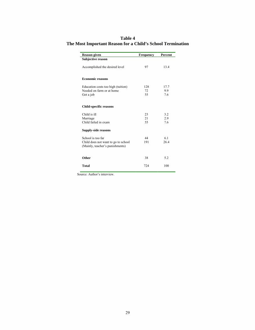
29

Table 4The Most Important Reason for a Child’s School Termination

Reason given Frequency PercentSubjective reason

Accomplished the desired level 97 13.4

Economic reasons

Education costs too high (tuition) 128 17.7Needed on farm or at home 72 9.9Got a job 55 7.6

Child-specific reasons

Child is ill 23 3.2Marriage 21 2.9Child failed in exam 55 7.6

Supply-side reasons

School is too far 44 6.1Child does not want to go to school(Mainly, teacher’s punishments)

191 26.4

Other 38 5.2

Total 724 100

Source: Author’s interview.

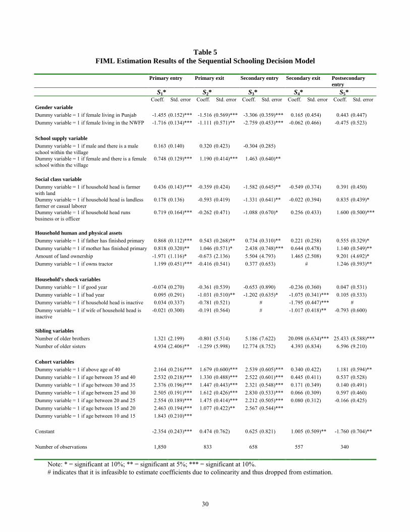
30

Table 5FIML Estimation Results of the Sequential Schooling Decision Model

Primary entry Primary exit Secondary entry Secondary exit Postsecondaryentry

S1* S2* S3* S4* S5*Coeff. Std. error Coeff. Std. error Coeff. Std. error Coeff. Std. error Coeff. Std. error

Gender variableDummy variable = 1 if female living in Punjab -1.455 (0.152)*** -1.516 (0.569)*** -3.306 (0.359)*** 0.165 (0.454) 0.443 (0.447)Dummy variable = 1 if female living in the NWFP -1.716 (0.134)*** -1.111 (0.571)** -2.759 (0.453)*** -0.062 (0.466) -0.475 (0.523)

School supply variableDummy variable = 1 if male and there is a maleschool within the village

0.163 (0.140) 0.320 (0.423) -0.304 (0.285)

Dummy variable = 1 if female and there is a femaleschool within the village

0.748 (0.129)*** 1.190 (0.414)*** 1.463 (0.640)**

Social class variableDummy variable = 1 if household head is farmerwith land

0.436 (0.143)*** -0.359 (0.424) -1.582 (0.645)** -0.549 (0.374) 0.391 (0.450)

Dummy variable = 1 if household head is landlessfarmer or casual laborer

0.178 (0.136) -0.593 (0.419) -1.331 (0.641)** -0.022 (0.394) 0.835 (0.439)*

Dummy variable = 1 if household head runsbusiness or is officer

0.719 (0.164)*** -0.262 (0.471) -1.088 (0.670)* 0.256 (0.433) 1.600 (0.500)***

Household human and physical assetsDummy variable = 1 if father has finished primary 0.868 (0.112)*** 0.543 (0.268)** 0.734 (0.310)** 0.221 (0.258) 0.555 (0.329)*Dummy variable = 1 if mother has finished primary 0.818 (0.320)** 1.046 (0.571)* 2.438 (0.748)*** 0.644 (0.478) 1.140 (0.549)**Amount of land ownership -1.971 (1.116)* -0.673 (2.136) 5.504 (4.793) 1.465 (2.508) 9.201 (4.692)*Dummy variable = 1 if owns tractor 1.199 (0.451)*** -0.416 (0.541) 0.377 (0.653) # 1.246 (0.593)**

Household’s shock variablesDummy variable = 1 if good year -0.074 (0.270) -0.361 (0.539) -0.653 (0.890) -0.236 (0.360) 0.047 (0.531)Dummy variable = 1 if bad year 0.095 (0.291) -1.031 (0.510)** -1.202 (0.635)* -1.075 (0.341)*** 0.105 (0.533)Dummy variable = 1 if household head is inactive 0.034 (0.337) -0.781 (0.521) # -1.795 (0.447)*** #Dummy variable = 1 if wife of household head isinactive

-0.021 (0.300) -0.191 (0.564) # -1.017 (0.418)** -0.793 (0.600)

Sibling variablesNumber of older brothers 1.321 (2.199) -0.801 (5.514) 5.186 (7.622) 20.098 (6.634)*** 25.433 (8.588)***Number of older sisters 4.934 (2.406)** -1.259 (5.998) 12.774 (8.752) 4.393 (6.834) 6.596 (9.210)

Cohort variablesDummy variable = 1 if above age of 40 2.164 (0.216)*** 1.679 (0.600)*** 2.539 (0.605)*** 0.340 (0.422) 1.181 (0.594)**Dummy variable = 1 if age between 35 and 40 2.532 (0.218)*** 1.330 (0.488)*** 2.522 (0.601)*** 0.445 (0.411) 0.537 (0.528)Dummy variable = 1 if age between 30 and 35 2.376 (0.196)*** 1.447 (0.443)*** 2.321 (0.548)*** 0.171 (0.349) 0.140 (0.491)Dummy variable = 1 if age between 25 and 30 2.505 (0.191)*** 1.612 (0.426)*** 2.830 (0.533)*** 0.066 (0.309) 0.597 (0.460)Dummy variable = 1 if age between 20 and 25 2.554 (0.189)*** 1.475 (0.414)*** 2.212 (0.505)*** 0.080 (0.312) -0.166 (0.425)Dummy variable = 1 if age between 15 and 20 2.463 (0.194)*** 1.077 (0.422)** 2.567 (0.544)***Dummy variable = 1 if age between 10 and 15 1.843 (0.210)***

Constant -2.354 (0.243)*** 0.474 (0.762) 0.625 (0.821) 1.005 (0.509)** -1.760 (0.704)**

Number of observations 1,850 833 658 557 340

Note: * = significant at 10%; ** = significant at 5%; *** = significant at 10%.# indicates that it is infeasible to estimate coefficients due to colinearity and thus dropped from estimation.

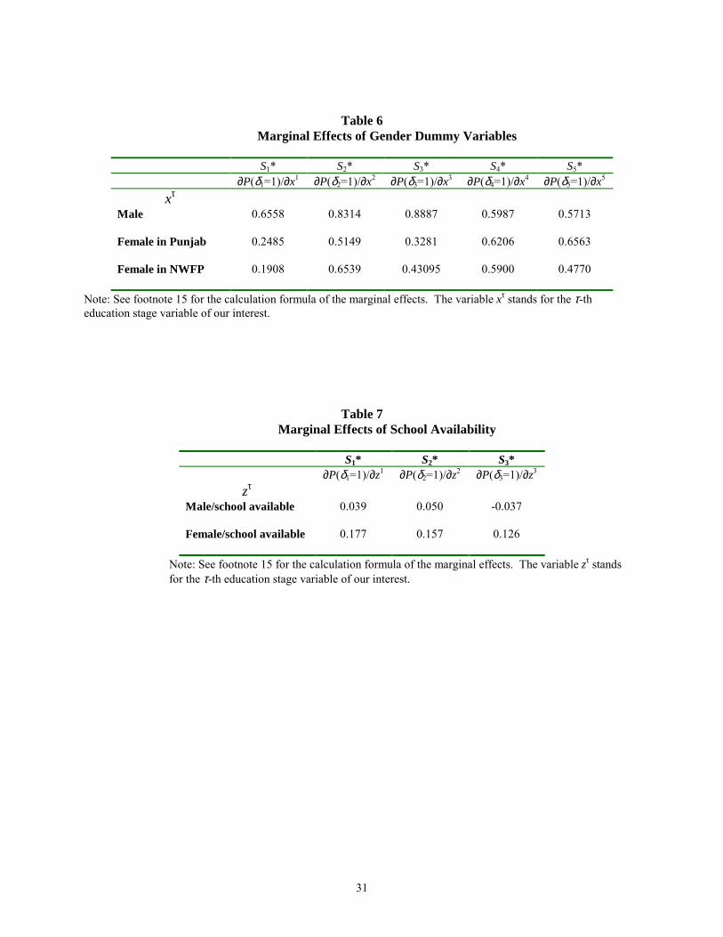
31

Table 6Marginal Effects of Gender Dummy Variables

S1* S2* S3* S4* S5*∂P(δ1=1)/∂x1 ∂P(δ2=1)/∂x2 ∂P(δ3=1)/∂x3 ∂P(δ4=1)/∂x4 ∂P(δ5=1)/∂x5

xτ

Male 0.6558 0.8314 0.8887 0.5987 0.5713

Female in Punjab 0.2485 0.5149 0.3281 0.6206 0.6563

Female in NWFP 0.1908 0.6539 0.43095 0.5900 0.4770

Note: See footnote 15 for the calculation formula of the marginal effects. The variable xτ stands for the τ-theducation stage variable of our interest.

Table 7Marginal Effects of School Availability

S1* S2* S3*∂P(δ1=1)/∂z1 ∂P(δ2=1)/∂z2 ∂P(δ3=1)/∂z3

zτ

Male/school available 0.039 0.050 -0.037

Female/school available 0.177 0.157 0.126

Note: See footnote 15 for the calculation formula of the marginal effects. The variable zτ standsfor the τ-th education stage variable of our interest.