Household schooling and child labor decisions in rural ...mnshafiq/M_Najeeb_Shafiq_(University_of_Pittsburgh... · Household schooling and child labor decisions in rural Bangladesh

Household schooling and child labor

decisions in rural Bangladesh

M. Najeeb Shafiq *

Department of Educational Leadership and Policy Studies, Indiana University,

201 North Rose Avenue, Bloomington, IN 47405, United States

Abstract

Using empirical methods, this paper examines household schooling and child labor decisions in rural

Bangladesh. The results suggest the following: poverty and low parental education are associated with lower

schooling and greater child labor; asset-owning households are more likely to have children combine child

labor with schooling; households choose the same activity for all children within the household, regardless

of gender; there is a weak association between direct costs and household decisions; finally, higher child

wages encourage households to practice child labor.

# 2007 Elsevier Inc. All rights reserved.

JEL classification : C35; D19; I29; J13

Keywords: Child labor; Education; Demography; Economic development; Bangladesh

1. Introduction

A household’s schooling and child labor decisions have several implications for the household

itself and society. By not enrolling children in school, a household prevents itself and its children

from benefiting from higher earnings (associated with educational attainment) in the future; for a

poor household, this diminishes its chances of escaping the vicious cycle of poverty (Ljungqvist,

1993). Not enrolling children in school also inhibits a household and its children from enjoying

the non-pecuniary benefits of schooling, such as improvements in patience, risk management

skills, and health (Becker & Mulligan, 1997; Sander, 1995). From a society’s perspective, lower

school enrollment undermine social cohesion, diminish political participation, encourage crime,

and lessen numerous other social benefits from having an educated populace (Behrman & Stacey,

Journal of Asian Economics 18 (2007) 946–966

* Tel.: +1 812 856 8235; fax: +1 812 856 8394.

E-mail address: [email protected].

1049-0078/$ – see front matter # 2007 Elsevier Inc. All rights reserved.

doi:10.1016/j.asieco.2007.07.003

mailto:[email protected]

http://dx.doi.org/10.1016/j.asieco.2007.07.003

1997). A household’s decision to practice child labor may expose its children to physical

injury and other health problems (Beegle, Dehejia, and Gatti, 2004; O’Donnell, Rosati, &

Doorslaer, 2002); furthermore, health problems harm children’s participation in school.

Consequently, household decisions to practice child labor eventually deprive society of

healthy and productive adult citizens. Nonetheless, many households in the developing world

(especially in rural areas) practice child labor for reasons of survival or saving the costs of

outside labor (Edmonds, 2007).

The troubling household- and social-level implications arising from household schooling

and child labor decisions are likely to be substantial in rural Bangladesh. Among the 27.4

million rural children in the 5–14 age-group, at least 4.8 million children are not enrolled in

school (most of whom are engaging in child labor) and a further 5.6 million children combine

schooling with child labor (refers to 2002–2003 figures; Bangladesh Bureau of Statistics,

2003). This persistence of household underinvestment in schooling and practice of child labor

continues despite respectable private returns to schooling (7.1% for each year of schooling;

Asadullah, 2006), government and non-government initiatives at building schools and

keeping costs low, and nation-wide laws requiring compulsory primary school attendance and

banning child labor (for details on educational initiatives, see World Bank, 2000). Given the

household- and social-level consequences of not enrolling children in school and practicing

child labor, the purposes of this study are to understand the child-, household-, and village-

level characteristics associated with the schooling and child labor decisions of households in

rural Bangladesh, and addressing the implications of the results for educational and child

labor policies.1

2. Literature review

This section reviews some of the existing theoretical and empirical literature on household

schooling and child labor decisions from the developing world (for reviews, see Basu, 1999;

Brown, Deardorff, & Stern, 2002; Dar, Blunch, Kim, & Sasaki, 2002; Edmonds, 2007; Edmonds

& Pavcnik, 2005; Glewwe, 2002; Hannum & Buchmann, 2004; Udry, 2006).

Much theoretical and empirical research shows that household poverty either prevents

investment in schooling, or forces the practice of child labor (for survival), or both (Basu & Van,

1998; Edmonds, 2005; Edmonds & Pavcnik, 2005). Regarding poverty and schooling in South

Asia, Maitra (2003), Dreze and Kingdon (2001) and Holmes (2003) present evidence on the

negative association between poverty and schooling in rural areas of Bangladesh (the Matlab

area), India, and Pakistan. As for poverty and child labor in South Asia, Swaminathan (1998) and

Rossi and Rosati (2003) find associations between poverty and child labor in India and Pakistan;

however, Bhatty (1998) finds no association between poverty and child labor in rural India, and

Bhalotra and Heady (2003) reach the same conclusion with girls in rural Pakistan.

Arguably, the most consistent finding in theoretical and empirical research is that

underinvestment in schooling and the practice of child labor is a consequence of low parental

educational attainment (Dar et al., 2002). There are at least three possible reasons for greater

M.N. Shafiq / Journal of Asian Economics 18 (2007) 946–966 947

1 The following are some additional regional characteristics (for details, see World Bank and Asian Development Bank,

2003a,b): Bangladesh is small and densely populated country in South Asia. The population in 2000 was 140 million; of

this, 54 million were categorized as poor; of the total poor, 85.2% resided in rural areas; the average annual GDP per

capita in Bangladesh in 2000 was US$ 370.

parental education resulting in more schooling and less child labor. First, there may be a positive

correlation between parental education and children’s ability, which reduces the likelihood of a

child failing out of school. Second, educated parents raise the likelihood of a child remaining in

school by providing an environment conducive to learning (such as directly helping with

schoolwork) and being knowledgeable about children’s nutritional and health needs. Third,

during income shocks (such as unemployment and natural disasters), a household with educated

parents is less likely to pull a child out of school, practice child labor, or both because educated

workers have safety nets (such as insurance).

An objective of economic development is to enable poor households to acquire income-

generating assets. There is, however, curious evidence on the association between asset-

ownership and child labor. Bhalotra and Heady (2003) find that farm-owning households are

more likely to practice child labor in rural Ghana and rural Pakistan; Edmonds and Turk (2004)

find evidence from rural Vietnam that business-owning households are more likely to practice

child labor. This wealth paradox (as labeled by Bhalotra and Heady) is open to misinterpretation

unless the schooling activities of these children are also considered. That is, a household with a

farm or business assets may ask a child to help operate those assets (or supervise outside laborers

work on the assets), but that household is also more likely to send the child to school; it follows

that an asset-less household would be less likely to send its child to school. There remains cause

for concern because asset-ownership can encourage both more child labor and less schooling, as

Wydick (1999) finds among rural Guatemalan households.

There is substantial research on the intra-household resource allocation in developing

countries. There is, however, no research to my knowledge on the effect of other children’s

schooling and child labor activities (within the household) on a particular child (Strauss &

Thomas, 1995).

Existing research suggests that the direct and indirect costs of schooling affect household

schooling and child labor decisions. In the developing world, households face direct costs of

schooling, such as tuition, fees, donations, books, supplies, uniform, transportation, private

tutoring, and miscellaneous costs. In a survey, Tsang (1994) reports that direct costs are often a

heavy financial burden for households in developing countries. In response, major international

education initiatives such as the United Nations’ ‘‘Education for All’’ strongly consider reducing

or eliminating the direct costs of schooling in order to raise school enrolment and attainment rates

in developing countries (UNESCO, 2005). Deininger (2003) and Hazarika (2001) present

evidence from Uganda and Pakistan on direct costs discouraging household investment in

schooling., Grootaert (1999a), however, finds no association between direct costs and household

schooling and child labor decisions in rural Cote d’Ivoire. Regarding indirect costs of schooling,

Schultz (1960) and Rozenzweig and Evenson (1977) were among the first to discuss the

possibility of children’s opportunity costs discouraging household schooling decisions. More

recently, Duryea and Arends-Kuenning (2003) and Binder and Scrogin (1999) find evidence that

the rates of child labor are higher at times when children receive better pay in urban child labor

markets of Brazil and Mexico.

Accordingly, this study contributes by examining the following issues for households in rural

Bangladesh: whether poverty is associated with less schooling and more child labor; whether

asset-ownership is associated with less schooling and more child labor; whether the composition

and activities of other children within a household are associated with the schooling and child

labor decision towards a particular child; whether direct and indirect costs of schooling are

associated with less schooling and more child labor; and finally, whether households behave

differently towards boys and girls.

M.N. Shafiq / Journal of Asian Economics 18 (2007) 946–966948

3. Data and definitions

The data for this study comes from a typical multipurpose household survey: the Bangladesh

Household Income and Expenditure Survey 2000 (henceforth referred to as HIES 2000). The

HIES 2000, conducted in the year 2000, was a joint project of the Bangladesh Bureau of Statistics

and the World Bank, and followed a stratified and clustered survey strategy (i.e., allowing each

household in the population to have an equal probability of inclusion), and therefore nationally

representative. The survey questionnaire is based on the popular World Bank Living Standards

Measurement Surveys, with detailed person, household, and community-level data. Survey staffs

collected information on household composition, education, health, employment, asset-

ownership, consumption, and expenditure from urban and rural communities. The staffs also

collected community-level information for rural areas, such as commodity prices, location,

infrastructure, and wage rates. The rural sample of the HIES 2000 consists of 5,040 households

and 26,231 people.

For children, the HIES 2000 includes basic information on household members over the age

of five, such as school enrolment status, educational attainment, and work status. I use the

sample of children in the 6–15 age-group because six is the age when children are socially

encouraged to begin primary schooling (and therefore the start of the potential trade-offs

between schooling and child labor), and fifteen is the age when children are expected to finish

secondary school.2

I define schooling as children being enrolled in school, and define child labor as all forms of

work performed by children (i.e., within the child’s household or in the child labor market). To

determine whether a child engages in schooling, a binary value 1 is assigned if the child is

enrolled in school and zero is assigned otherwise. To determine a child laborer, a binary value 1 is

assigned to a child laborer, and 0 to a child who reportedly does not engage in child labor.

Following the HIES 2000 questionnaire, one is assigned for a child reported as having worked in

the past week, being available for work in the past week, or looking for work in the past week.

Along with all children in self-employment and wage work, some children who were not working

during the survey period are still assigned one if survey respondents claimed one of the following

reasons for the child not working: already have enough work (domestic or occupational),

temporarily sick, waiting to start a new job, or no work available. However, I am unable to

distinguish between domestic work (e.g., cooking and taking care of dependents) versus

fieldwork (e.g., working on a farm or business), and between own-household work versus market

work.3 All other children who are reportedly idle or only engage in schooling are assigned zero,

implying that they reportedly do not practice any form of child labor.

Using these definitions of schooling and child labor, I produce three household decisions on

schooling and child labor: SCHOOLONLY, COMBINE, and OS. The SCHOOLONLY category

consists of children who attend school and avoid child labor. Children in the COMBINE category

are those that combine schooling with child labor. Finally, the OS category includes children

whose only activity is child labor, or idle (i.e., reportedly involved in neither schooling nor child

labor). Any child can be categorized in one of the three child activity categories.


2 The education structure of Bangladesh involves 5 years of primary school, 5 years of secondary school, 2 years of

upper secondary school, and at least 3 years of higher education.3 The HIES 2000 also has also patchy information on time-use, and no information on school-outcomes and physical

injuries sustained from child labor, thereby limiting inquiry into trade-offs between child labor and education and health.

4. Methodology

Much of the theoretical research on a household’s child activity decision originates from the

seminal pieces on fertility by Becker (1960) and Becker and Lewis (1973). In the original

models, the household’s child activity decision involves a constrained (indirect) utility

maximization problem, where a household faces tradeoffs between the number of children,

investment in children’s human capital, and current consumption of goods. Testing these and

subsequent models using econometric analysis has traditionally been difficult because of the

dearth of child labor data in multipurpose household surveys. Indeed, early econometric

approaches were limited to binomial logit or probit specifications that assumed child labor as the

inverse of schooling—which is problematic because it ignores the possibility of a child

combining child labor and schooling, or the possibility of a child being idle. Efforts at collecting

basic child labor data in multipurpose household surveys increased in the 1990s largely because

of International Labour Organisation led efforts (Asgharie, 1993), and the MNL emerged as a

popular specification in response to the basic data on child labor and schooling (Edmonds, 2007).

The foundation for the estimation methodology in this study comes from Maitra and Ray

(2002). The following latent variable model describes the household’s decision to enroll a child

in school:

S�i ¼ X2ibþ e2i (1)

where S�i is the utility attained by the household from having child i engage in schooling, Xi a

vector of child-, household-, and community-level characteristics that determine S�i , and e2i is a

random error with zero mean and unit variance. For schooling, the researcher observes the

following binary variable:

Si ¼ 1 if the household enrolls the child in school ðS�i > 0Þ; 0; otherwise (2)

Similarly, the following latent variable model describes the household’s decision to choose

child labor as the child’s activity:

L�i ¼ X1ibþ e1i (3)

where L�i is the utility attained by the household by having child i in engage in child labor, Xi a

vector of child-, household-, and community-level characteristics that determine L�i , and e1i is a

random error, with zero mean and unit variance. In practice, however, the researcher observes

neither the decision-making process nor L�i . Rather, the researcher only observes the following

binary variable:

Li ¼ 1 if the households makes the child work ðL�i > 0Þ; 0; otherwise (4)

Given this study’s emphasis on SCHOOLONLY, COMBINE, and OS, the two-equation

system (given by Eqs. (1) and (3)) into an observable form Y, involving the three child activity

decisions:

SCHOOLONLY) Yi ¼ 1 : L�i � 0; S�i > 0

COMBINE) Yi ¼ 2 : L�i > 0; S�i > 0

OS) Yi ¼ 3 : S�i

� 0ðwith L�i > 0 implying ‘only child labor’; and L�i � 0 implying ‘idle’Þ


The estimated equation is given by

Yi ¼ Xibþ ei (5)

where Yi is the utility attained by the household from having child i engage in a particular child

labor and schooling decision, Xi a vector of child-, household-, and community-level character-

istics that determine Yi, and ei is a random error with zero mean and unit variance.

The MNL specification assumes that a household simultaneously compares the expected

utilities from SCHOOLONLY, COMBINE, and OS. The unordered nature of the categorical

variables in a MNL specification indicate that a household makes its child activity decision in a

single step. The key characteristic of the MNL approach is that it makes no assumptions about the

household’s child activity preferences, so any of the three child activities can be a particular

household’s most preferred activity. The equation of the MNL specification is

PrðYiÞ ¼ePK

k¼1b jkXk

1þP3

j¼1 ePK

k¼1b jkXk

; Yi ¼ 1; 2; 3 (6)

where parameters b have two subscripts in the model, k for distinguishing X explanatory

variables. The subscript j indicates how there are three sets of b estimates, implying that the total

number of parameter estimates will be (3 � K). There is a single estimation process, using the

entire sample of children. A weakness of the MNL specification is that it requires the

independence of irrelevant alternatives (IIA) assumption, where the odds ratios derived from

the model remain the same, irrespective of the number of choices offered (Maddala, 1983). That

is, the IIA requires that the relative probability of choosing between two alternatives is unaffected

by the presence of a third alternative. In practice, this assumption is incorrect if the choices are

close substitutes, as are schooling and child labor alternatives. Consequently, the MNL model can

overestimate the selection probabilities of the child activity decisions.4 The appropriateness of

the MNL specification can be tested using the Hausman–McFadden specification test for the

presence of IIA (Hausman & McFadden, 1984).

5. Results

5.1. Descriptive statistics

The sample of analysis refers to the number of children, but can also refer to the number of

household child labor and schooling decisions. Figs. 1 and 2 illustrate the activities of boys and

girls by age. Most households decide on SCHOOLONLY, and this decision peaks around the ages

of 8 and 9. The COMBINE decision remains small and steady across the age-groups. The

increasing proportion of OS children from age of 10 indicates that many households break the

compulsory primary school attendance law by pulling children out of school before primary

school completion. Overall, the proportion of child laborers (i.e., those in the COMBINE and OS

categories) may be underreported because households do not consider domestic work as child

labor, or because households are hesitant to report child labor practices to survey collectors (as

discussed earlier, child labor is illegal in Bangladesh; Biggeri, Guarcello, Lyon, & Rosati, 2003).


4 Grootaert and Patrinos (1999) note that using a multinomial probit model (in which the residuals have a multivariate

normal distribution and which is not subject to the IIA) to get around this problem is not practical because computational

difficulties only allow a small number of alternatives.

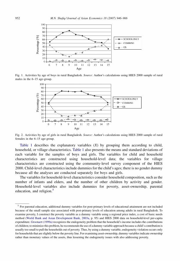
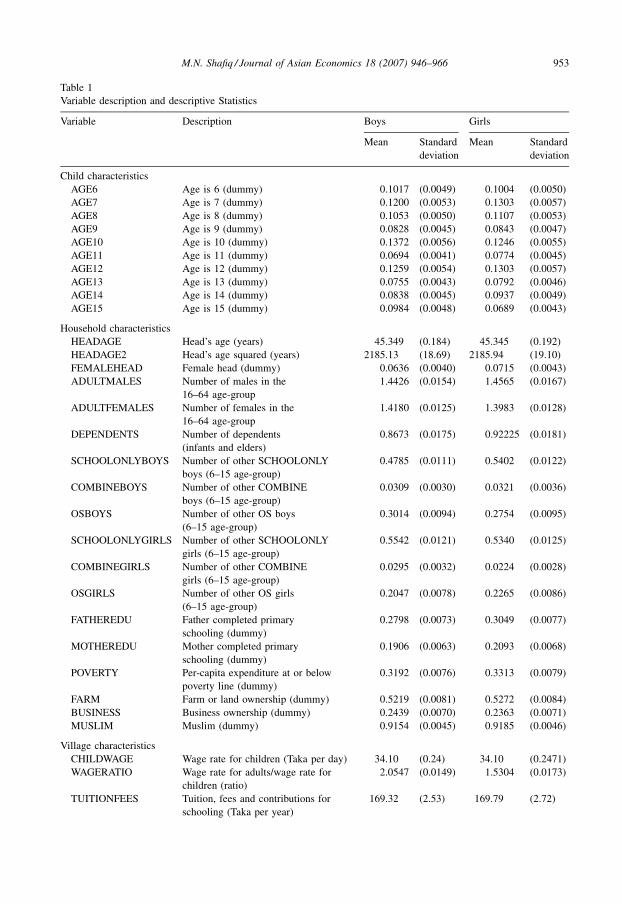
Table 1 describes the explanatory variables (X) by grouping them according to child,

household, or village characteristics. Table 1 also presents the means and standard deviations of

each variable for the samples of boys and girls. The variables for child and household

characteristics are constructed using household-level data; the variables for village

characteristics are constructed using the community-level survey component of the HIES

2000. Child-level characteristics include dummies for the child’s ages; there is no gender dummy

because all the analyses are conducted separately for boys and girls.

The variables for household-level characteristics consider household composition, such as the

number of infants and elders, and the number of other children by activity and gender.

Household-level variables also include dummies for poverty, asset-ownership, parental

education, and religion.5


Fig. 1. Activities by age of boys in rural Bangladesh. Source: Author’s calculations using HIES 2000 sample of rural

males in the 6–15 age-group.

Fig. 2. Activities by age of girls in rural Bangladesh. Source: Author’s calculations using HIES 2000 sample of rural

females in the 6–15 age-group.

5 For parental education, additional dummy variables for post-primary levels of educational attainment are not included

because of the small sample size associated with post-primary levels of education among adults in rural Bangladesh. To

examine poverty, I construct the poverty variable as a dummy variable using a regional price index, a cost of basic needs

method (World Bank and Asian Development Bank, 2003a, p. 95) and HIES 2000 data on household-level per-capita

expenditure. Grootaert (1999a) recognizes the endogeneity problem that the household’s income includes the contributions

of children; to minimize this problem, he recommends the use of a dummy variable approach because a child’s contribution is

usually too small to pull the households out of poverty. Thus, by using a dummy variable, endogeneity violation occurs only

for households that are slightly below the poverty line. For examining asset-ownership, dummy variables indicate ownership

rather than monetary values of the assets, thus lessening the endogeneity issues with also addressing poverty.


Table 1

Variable description and descriptive Statistics

Variable Description Boys Girls

Mean Standard

deviation

Mean Standard

deviation

Child characteristics

AGE6 Age is 6 (dummy) 0.1017 (0.0049) 0.1004 (0.0050)

AGE7 Age is 7 (dummy) 0.1200 (0.0053) 0.1303 (0.0057)

AGE8 Age is 8 (dummy) 0.1053 (0.0050) 0.1107 (0.0053)

AGE9 Age is 9 (dummy) 0.0828 (0.0045) 0.0843 (0.0047)

AGE10 Age is 10 (dummy) 0.1372 (0.0056) 0.1246 (0.0055)

AGE11 Age is 11 (dummy) 0.0694 (0.0041) 0.0774 (0.0045)

AGE12 Age is 12 (dummy) 0.1259 (0.0054) 0.1303 (0.0057)

AGE13 Age is 13 (dummy) 0.0755 (0.0043) 0.0792 (0.0046)

AGE14 Age is 14 (dummy) 0.0838 (0.0045) 0.0937 (0.0049)

AGE15 Age is 15 (dummy) 0.0984 (0.0048) 0.0689 (0.0043)

Household characteristics

HEADAGE Head’s age (years) 45.349 (0.184) 45.345 (0.192)

HEADAGE2 Head’s age squared (years) 2185.13 (18.69) 2185.94 (19.10)

FEMALEHEAD Female head (dummy) 0.0636 (0.0040) 0.0715 (0.0043)

ADULTMALES Number of males in the

16–64 age-group

1.4426 (0.0154) 1.4565 (0.0167)

ADULTFEMALES Number of females in the

16–64 age-group

1.4180 (0.0125) 1.3983 (0.0128)

DEPENDENTS Number of dependents

(infants and elders)

0.8673 (0.0175) 0.92225 (0.0181)

SCHOOLONLYBOYS Number of other SCHOOLONLY

boys (6–15 age-group)

0.4785 (0.0111) 0.5402 (0.0122)

COMBINEBOYS Number of other COMBINE

boys (6–15 age-group)

0.0309 (0.0030) 0.0321 (0.0036)

OSBOYS Number of other OS boys

(6–15 age-group)

0.3014 (0.0094) 0.2754 (0.0095)

SCHOOLONLYGIRLS Number of other SCHOOLONLY

girls (6–15 age-group)

0.5542 (0.0121) 0.5340 (0.0125)

COMBINEGIRLS Number of other COMBINE

girls (6–15 age-group)

0.0295 (0.0032) 0.0224 (0.0028)

OSGIRLS Number of other OS girls

(6–15 age-group)

0.2047 (0.0078) 0.2265 (0.0086)

FATHEREDU Father completed primary

schooling (dummy)

0.2798 (0.0073) 0.3049 (0.0077)

MOTHEREDU Mother completed primary

schooling (dummy)

0.1906 (0.0063) 0.2093 (0.0068)

POVERTY Per-capita expenditure at or below

poverty line (dummy)

0.3192 (0.0076) 0.3313 (0.0079)

FARM Farm or land ownership (dummy) 0.5219 (0.0081) 0.5272 (0.0084)

BUSINESS Business ownership (dummy) 0.2439 (0.0070) 0.2363 (0.0071)

MUSLIM Muslim (dummy) 0.9154 (0.0045) 0.9185 (0.0046)

Village characteristics

CHILDWAGE Wage rate for children (Taka per day) 34.10 (0.24) 34.10 (0.2471)

WAGERATIO Wage rate for adults/wage rate for

children (ratio)

2.0547 (0.0149) 1.5304 (0.0173)

TUITIONFEES Tuition, fees and contributions for

schooling (Taka per year)

169.32 (2.53) 169.79 (2.72)

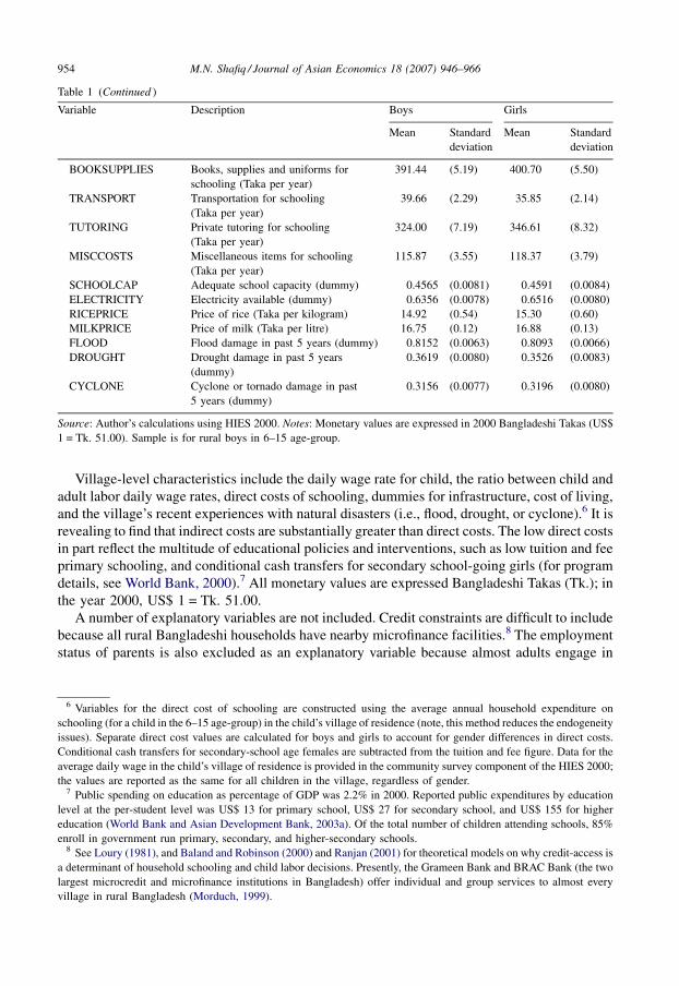
Village-level characteristics include the daily wage rate for child, the ratio between child and

adult labor daily wage rates, direct costs of schooling, dummies for infrastructure, cost of living,

and the village’s recent experiences with natural disasters (i.e., flood, drought, or cyclone).6 It is

revealing to find that indirect costs are substantially greater than direct costs. The low direct costs

in part reflect the multitude of educational policies and interventions, such as low tuition and fee

primary schooling, and conditional cash transfers for secondary school-going girls (for program

details, see World Bank, 2000).7 All monetary values are expressed Bangladeshi Takas (Tk.); in

the year 2000, US$ 1 = Tk. 51.00.

A number of explanatory variables are not included. Credit constraints are difficult to include

because all rural Bangladeshi households have nearby microfinance facilities.8 The employment

status of parents is also excluded as an explanatory variable because almost adults engage in


Table 1 (Continued )

Variable Description Boys Girls

Mean Standard

deviation

Mean Standard

deviation

BOOKSUPPLIES Books, supplies and uniforms for

schooling (Taka per year)

391.44 (5.19) 400.70 (5.50)

TRANSPORT Transportation for schooling

(Taka per year)

39.66 (2.29) 35.85 (2.14)

TUTORING Private tutoring for schooling

(Taka per year)

324.00 (7.19) 346.61 (8.32)

MISCCOSTS Miscellaneous items for schooling

(Taka per year)

115.87 (3.55) 118.37 (3.79)

SCHOOLCAP Adequate school capacity (dummy) 0.4565 (0.0081) 0.4591 (0.0084)

ELECTRICITY Electricity available (dummy) 0.6356 (0.0078) 0.6516 (0.0080)

RICEPRICE Price of rice (Taka per kilogram) 14.92 (0.54) 15.30 (0.60)

MILKPRICE Price of milk (Taka per litre) 16.75 (0.12) 16.88 (0.13)

FLOOD Flood damage in past 5 years (dummy) 0.8152 (0.0063) 0.8093 (0.0066)

DROUGHT Drought damage in past 5 years

(dummy)

0.3619 (0.0080) 0.3526 (0.0083)

CYCLONE Cyclone or tornado damage in past

5 years (dummy)

0.3156 (0.0077) 0.3196 (0.0080)

Source: Author’s calculations using HIES 2000. Notes: Monetary values are expressed in 2000 Bangladeshi Takas (US$

1 = Tk. 51.00). Sample is for rural boys in 6–15 age-group.

6 Variables for the direct cost of schooling are constructed using the average annual household expenditure on

schooling (for a child in the 6–15 age-group) in the child’s village of residence (note, this method reduces the endogeneity

issues). Separate direct cost values are calculated for boys and girls to account for gender differences in direct costs.

Conditional cash transfers for secondary-school age females are subtracted from the tuition and fee figure. Data for the

average daily wage in the child’s village of residence is provided in the community survey component of the HIES 2000;

the values are reported as the same for all children in the village, regardless of gender.7 Public spending on education as percentage of GDP was 2.2% in 2000. Reported public expenditures by education

level at the per-student level was US$ 13 for primary school, US$ 27 for secondary school, and US$ 155 for higher

education (World Bank and Asian Development Bank, 2003a). Of the total number of children attending schools, 85%

enroll in government run primary, secondary, and higher-secondary schools.8 See Loury (1981), and Baland and Robinson (2000) and Ranjan (2001) for theoretical models on why credit-access is

a determinant of household schooling and child labor decisions. Presently, the Grameen Bank and BRAC Bank (the two

largest microcredit and microfinance institutions in Bangladesh) offer individual and group services to almost every

village in rural Bangladesh (Morduch, 1999).

productive activities in a poor rural economy, either through wage employment, self-

employment, or inside their own household.

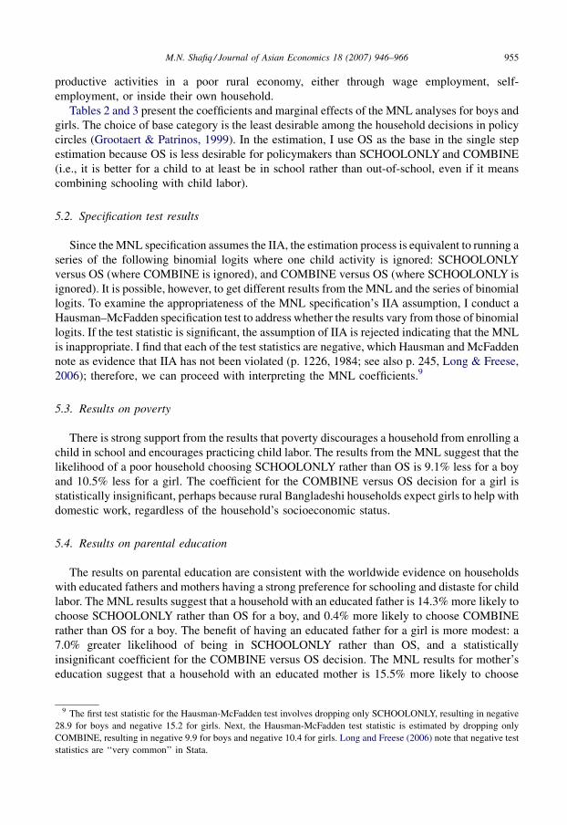
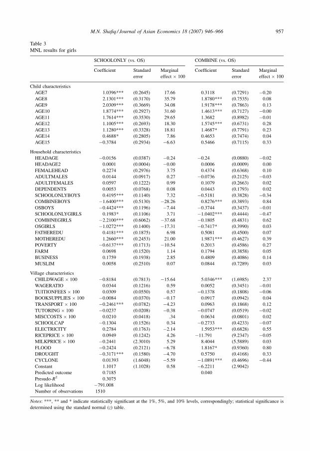
Tables 2 and 3 present the coefficients and marginal effects of the MNL analyses for boys and

girls. The choice of base category is the least desirable among the household decisions in policy

circles (Grootaert & Patrinos, 1999). In the estimation, I use OS as the base in the single step

estimation because OS is less desirable for policymakers than SCHOOLONLY and COMBINE

(i.e., it is better for a child to at least be in school rather than out-of-school, even if it means

combining schooling with child labor).

5.2. Specification test results

Since the MNL specification assumes the IIA, the estimation process is equivalent to running a

series of the following binomial logits where one child activity is ignored: SCHOOLONLY

versus OS (where COMBINE is ignored), and COMBINE versus OS (where SCHOOLONLY is

ignored). It is possible, however, to get different results from the MNL and the series of binomial

logits. To examine the appropriateness of the MNL specification’s IIA assumption, I conduct a

Hausman–McFadden specification test to address whether the results vary from those of binomial

logits. If the test statistic is significant, the assumption of IIA is rejected indicating that the MNL

is inappropriate. I find that each of the test statistics are negative, which Hausman and McFadden

note as evidence that IIA has not been violated (p. 1226, 1984; see also p. 245, Long & Freese,

2006); therefore, we can proceed with interpreting the MNL coefficients.9

5.3. Results on poverty

There is strong support from the results that poverty discourages a household from enrolling a

child in school and encourages practicing child labor. The results from the MNL suggest that the

likelihood of a poor household choosing SCHOOLONLY rather than OS is 9.1% less for a boy

and 10.5% less for a girl. The coefficient for the COMBINE versus OS decision for a girl is

statistically insignificant, perhaps because rural Bangladeshi households expect girls to help with

domestic work, regardless of the household’s socioeconomic status.

5.4. Results on parental education

The results on parental education are consistent with the worldwide evidence on households

with educated fathers and mothers having a strong preference for schooling and distaste for child

labor. The MNL results suggest that a household with an educated father is 14.3% more likely to

choose SCHOOLONLY rather than OS for a boy, and 0.4% more likely to choose COMBINE

rather than OS for a boy. The benefit of having an educated father for a girl is more modest: a

7.0% greater likelihood of being in SCHOOLONLY rather than OS, and a statistically

insignificant coefficient for the COMBINE versus OS decision. The MNL results for mother’s

education suggest that a household with an educated mother is 15.5% more likely to choose


9 The first test statistic for the Hausman-McFadden test involves dropping only SCHOOLONLY, resulting in negative

28.9 for boys and negative 15.2 for girls. Next, the Hausman-McFadden test statistic is estimated by dropping only

COMBINE, resulting in negative 9.9 for boys and negative 10.4 for girls. Long and Freese (2006) note that negative test

statistics are ‘‘very common’’ in Stata.


Table 2

MNL results for boys

SCHOOLONLY (vs. OS) COMBINE (vs. OS)

Coefficient Standard

error

Marginal

effect � 100


error

Marginal

effect � 100


AGE7 0.5877*** (0.2191) 12.04 1.9092*** (0.7767) 0.88

AGE8 1.5121*** (0.2391) 31.90 2.5792*** (0.8109) 0.90

AGE9 1.9198*** (0.2810) 40.98 2.0565*** (0.9010) 0.43

AGE10 1.2842*** (0.2194) 26.82 2.8555*** (0.7686) 1.15

AGE11 1.1938*** (0.2681) 25.07 2.3236*** (0.8582) 0.88

AGE12 0.4870*** 0.2133 9.89 1.7841*** (0.8106) 0.85

AGE13 �0.0958 (0.2474) �2.93 2.1197*** (0.7929) 1.27

AGE14 �0.4379* (0.2387) �10.20 1.6593*** (0.8134) 1.14

AGE15 �1.1168*** (0.2309) �24.57 0.6326 (0.8092) 0.81


HEADAGE �0.0192 (0.0305) �0.41 �0.0294 (0.0734) �0.01

HEADAGE2 0.0001 (0.0003) 0.00 0.0003 (0.0007) 0.00

FEMALEHEAD �0.3812 (0.2506) �8.39 0.2348 (0.5331) 0.29

ADULTMALES �0.0316 (0.0722) 0.60 �0.2200 (0.1714) �0.12

ADULTFEMALES 0.1286 (0.0974) 2.75 0.1228 (0.1984) 0.02

DEPENDENTS �0.0429 (0.0556) �0.99 0.1612 (0.1293) 0.11

SCHOOLONLYBOYS 0.1173 (0.0893) 2.66 �0.2778 (0.2559) �0.21

COMBINEBOYS �0.8024*** (0.3596) �17.95 1.2096*** (0.3644) 1.02

OSBOYS �0.7457*** (0.0913) �16.02 �0.5532*** (0.2739) �0.25

SCHOOLONLYGIRLS 0.3377*** (0.0817) 7.81 �1.1460*** (0.3764) �0.80

COMBINEGIRLS �0.5697 (0.4259) �13.32 2.2980*** (0.4056) 1.57

OSGIRLS �0.4588*** (0.1112) �9.85 �0.3449 (0.3145) �0.02

FATHEREDU 0.6783*** (0.1514) 14.32 1.1156*** (0.3309) 0.38

MOTHEREDU 0.7239*** (0.1843) 15.51 0.6119* (0.3535) 0.07

POVERTY �0.4344*** (0.1263) �9.10 �0.9030*** (0.3649) �0.35

FARM 0.6097*** (0.1149) 13.03 0.6112*** (0.3030) 0.11

BUSINESS �0.0138 (0.1319) �0.41 0.2862 (0.29311) 0.17

MUSLIM �0.3896 (0.2081) �8.55 0.1669 (0.5325) 0.25


CHILDWAGEx100 �0.5519 (0.6419) �13.20 2.9671* (1.5047) 1.95

WAGERATIO 0.0670 (0.0898) 1.31 0.3684 (0.2309) 0.18

TUITIONFEES � 100 �0.0024 (0.0531) 0.07 0.0552 (0.1357) 0.03

BOOKSUPPLIES � 100 0.0157 (0.0324) 0.0 0.1106 (0.0799) 0.06

TRANSPORT � 100 �0.0145 (0.0411) �0.29 �0.0577 (0.1199) �0.03

TUTORING � 100 �0.0022 (0.0166) 0.00 �0.1300*** (0.0589) 0.09

MISCCOSTS � 100 0.0010 (0.0455) �0.05 0.1724*** (0.0918) 0.10

SCHOOLCAP 0.0824 (0.1136) 1.92 �0.3216 (0.2974) �0.22

ELECTRICITY 0.2855*** (0.1206) 6.12 0.2281 (0.3296) 0.02

RICEPRICE � 100 0.0573 (0.1194) 9.73 �21.306*** (8.9284) �12.44

MILKPRICE � 100 �0.5634 (1.0360) 112.91 2.9109 (3.4257) �1.47

FLOOD 0.0333 (0.1658) 0.84 �0.2870 (0.3765) �0.18

DROUGHT �0.1794 (0.1149) �3.69 �0.5421* (0.2981) �0.24

CYCLONE �0.0520 (0.1234) �1.00 �0.3366 (0.3616) �0.18

Constant 0.6904 (0.8651) �2.3208 (2.2778)

Predicted outcome 0.6796 0.0059

Presudo-R2 0.2778

Log likelihood �1330.633

Number of observations 2229

Notes: ***, ** and * indicate statistically significant at the 1%, 5%, and 10% levels, correspondingly; statistical significance is

determined using the standard normal (z) table.


Table 3

MNL results for girls

SCHOOLONLY (vs. OS) COMBINE (vs. OS)


error

Marginal

effect � 100


error

Marginal

effect � 100


AGE7 1.0396*** (0.2645) 17.66 0.3118 (0.7291) �0.20

AGE8 2.1301*** (0.3170) 35.79 1.8780*** (0.7535) 0.08

AGE9 2.0309*** (0.3669) 34.08 1.9178*** (0.7863) 0.13

AGE10 1.8774*** (0.2927) 31.60 1.4613*** (0.7127) �0.00

AGE11 1.7614*** (0.3530) 29.65 1.3682 (0.8982) �0.01

AGE12 1.1005*** (0.2693) 18.30 1.5745*** (0.6731) 0.28

AGE13 1.1280*** (0.3328) 18.81 1.4687* (0.7791) 0.23

AGE14 0.4688* (0.2805) 7.86 0.4653 (0.7474) 0.04

AGE15 �0.3784 (0.2934) �6.63 0.5466 (0.7115) 0.33


HEADAGE �0.0156 (0.0387) �0.24 �0.24 (0.0880) �0.02

HEADAGE2 0.0001 (0.0004) �0.00 0.0006 (0.0009) 0.00

FEMALEHEAD 0.2274 (0.2976) 3.75 0.4374 (0.6368) 0.10

ADULTMALES 0.0144 (0.0917) 0.27 �0.0736 (0.2125) �0.03

ADULTFEMALES 0.0597 (0.1222) 0.99 0.1079 (0.2663) 0.02

DEPENDENTS 0.0053 (0.0768) 0.08 0.0443 (0.1793) 0.02

SCHOOLONLYBOYS 0.4195*** (0.1140) 7.32 �0.5181 (0.3828) �0.34

COMBINEBOYS �1.6400*** (0.5130) �28.26 0.8276*** (0.3893) 0.84

OSBOYS �0.4424*** (0.1196) �7.44 �0.3744 (0.3437) �0.01

SCHOOLONLYGIRLS 0.1983* (0.1106) 3.71 �1.0402*** (0.4444) �0.47

COMBINEGIRLS �2.2100*** (0.6062) �37.68 �0.1805 (0.4831) 0.62

OSGIRLS �1.0272*** (0.1400) �17.31 �0.7417* (0.3990) 0.03

FATHEREDU 0.4181*** (0.1875) 6.98 0.5081 (0.4500) 0.07

MOTHEREDU 1.2660*** (0.2453) 21.00 1.9871*** (0.4627) 0.39

POVERTY �0.6137*** (0.1713) �10.54 0.2013 (0.4586) 0.27

FARM 0.0698 (0.1520) 1.14 0.1794 (0.3858) 0.05

BUSINESS 0.1759 (0.1938) 2.85 0.4809 (0.4086) 0.14

MUSLIM 0.0058 (0.2510) 0.07 0.0844 (0.7289) 0.03


CHILDWAGE � 100 �0.8184 (0.7813) �15.64 5.0346*** (1.6985) 2.37

WAGERATIO 0.0344 (0.1216) 0.59 0.0052 (0.3451) �0.01

TUITIONFEES � 100 0.0309 (0.0550) 0.57 �0.1378 (0.1808) �0.06

BOOKSUPPLIES � 100 �0.0084 (0.0370) �0.17 0.0917 (0.0942) 0.04

TRANSPORT � 100 �0.2461*** (0.0782) �4.23 0.0963 (0.1868) 0.12

TUTORING � 100 �0.0237 (0.0208) �0.38 �0.0747 (0.0519) �0.02

MISCCOSTS � 100 0.0210 (0.0418) .34 0.0634 (0.0801) 0.02

SCHOOLCAP �0.1304 (0.1526) 0.34 �0.2733 (0.4233) �0.07

ELECTRICITY 0.2784 (0.1763) �2.14 1.5953*** (0.6828) 0.55

RICEPRICE � 100 0.0949 (0.1242) 4.26 �11.791 (9.2347) �0.05

MILKPRICE � 100 �0.2441 (2.3010) 5.29 8.4044 (5.5889) 0.03

FLOOD �0.2424 (0.2121) �6.78 1.8167* (0.9360) 0.80

DROUGHT �0.3171*** (0.1580) �4.70 0.5750 (0.4168) 0.33

CYCLONE 0.01393 (1.6048) �5.59 �1.0891*** (0.4696) �0.44

Constant 1.1017 (1.1028) 0.58 �6.2211 (2.9042)


Presudo-R2 0.3075

Log likelihood �791.008

Number of observations 1510



SCHOOLONLY rather than OS for its boy, and only 0.1% more likely to choose COMBINE

rather than OS for a boy. The benefit of having an educated mother for a girl is larger, as a

household is 21.0% more likely to choose SCHOOLONLY rather than OS, and COMBINE rather

than OS by just 0.4%.

5.5. Results on asset-ownership

The results call for a careful interpretation of the wealth paradox: while there is a positive

association between household asset-ownership and child labor, those asset-owning households

are more likely to send children to school. Furthermore, asset-owning households appear to have

a greater preference for SCHOOLONLY: for a boy, the MNL results show that a farm or land-

owning household is 13.0% more likely to choose SCHOOLONLY rather than OS, and 0.1%

more likely to choose COMBINE rather than OS. For a girl, the MNL results suggest that

business-owning household is 3.6% more likely to choose COMBINE rather OS.

5.6. Results on intra-household decisions

The number and activities of other children is strongly associated with a household’s decision

toward a particular child. Specifically, the results imply that households in rural Bangladesh

prefer to choose the same activity for all children within the household, regardless of gender. The

results suggest that each additional girl in SCHOOLONLY increases the likelihood of a boy

being in SCHOOLONLY by 7.8%; for each additional child who is not in SCHOOLONLY, the

household’s likelihood of choosing SCHOOLONLY for the boy is between 9.9% and 18.0% less.

The COMBINE decision for a boy shows that each additional boy and girl in COMBINE is

associated with 1.0% and 1.6% greater likelihoods of the household choosing COMBINE rather

than OS. Similarly, the results for girls show that an additional boy and girl in SCHOOLONLY is

associated with a 7.3% and 3.7% greater likelihood of the household choosing SCHOOLONLY

rather than COMBINE; for each additional child in a non-SCHOOLONLY activity, a girl’s the

likelihood of being in SCHOOLONLY rather than OS is between 7.4% and 37.7% less. For the

COMBINE versus OS decision for a girl, the results suggest that each additional boy in

COMBINE increases the likelihood by 0.8%; each additional child in a non-COMBINE category

reduces the likelihood of a household choosing COMBINE rather than OS for a girl by under

0.5%.

5.7. Results on the indirect cost of schooling

The results on indirect costs indicate that a household in a village with a higher daily child

wage rate is more likely to invest in schooling but is unwilling to forego child labor earnings,

especially in the case of girls. The results suggest that a household in a village with Tk. 10 higher

daily child wage rate (corresponding to 19.3% increase in the average daily wage rate for a child

in rural Bangladesh) is 2.0% and 2.4% more likely to choose COMBINE rather than OS for a boy

and a girl.

5.8. Results on the direct cost of schooling

There are limited statistically significant associations between the direct costs of schooling

and household decisions. The results suggest that an annual rise of Tk. 100 (which corresponds to


approximately 9.6% and 9.3% of average annual total direct costs for a boy and girl) in

transportation costs reduces the likelihood of a household choosing SCHOOLONLY rather than

COMBINE for a girl by 4.2%. For the COMBINE versus OS decision for a boy, a Tk. 100

increase in private tutoring cost is associated with 0.1% less likelihood; the association between

miscellaneous costs is even smaller but (unexpectedly) positive. This result for a girl offers some

support for Arends-Kuenning and Amin’s (2004) study of two rural Bangladeshi villages, where

they observe that direct costs affect household secondary school decisions towards girls. There is

also some support for worldwide evidence in Bray (1999), with private tutoring costs

discouraging households to enroll boys to school. Overall, the probable explanation for small

magnitudes is that educational policies in rural Bangladesh have succeeded in keeping direct cost

levels relatively low: as a percentage of the average annual per-capita expenditure in rural

Bangladesh, the average annual direct cost is 11.6% for a boy and 12.0% for a girl.

5.9. Other results

There is some evidence that the number of adults in the household reduces the need to send a

child to work. The results also show that children in villages with electricity are more likely to

choose SCHOOLONLY (rather than OS) for a boy, perhaps because economically developed

villages discourage child labor, or because the adults are more productive (from being able to use

electric-powered tools, and lighting to work in the evening), and therefore do need assistance

from boys. For a girl, there is greater likelihood of a household choosing COMBINE (rather than

OS), possibly because electricity facilitates work in the daytime and provides lighting to study in

the evening. In terms of the cost of living, the prices of rice and milk decrease the likelihood of

schooling for a boy. Lastly, the recent occurrence of natural disasters reduces the likelihood of a

household enrolling its child in school.

5.10. Differences in results by gender

The results provide some evidence of rural Bangladeshi households behaving differently

towards boys and girls. Household decisions towards girl are less sensitive to poverty, possibly

because rural Bangladeshi girls help with domestic work regardless of their household’s

socioeconomic status. Father’s education matters less for girls than it does for boys, while

mother’s education matters more for girls. There is also evidence that ownership of farm or land is

associated with household decisions towards boys, while ownership of business is associated

with household decisions towards girls. In addition, households are also more sensitive to

transportation costs of schooling for girls, perhaps out of greater safety concerns for girls.

5.11. Evidence from an alternative empirical specification

As frequently encountered in empirical research from all disciplines, the results and policy

implications drawn from the results can vary depending on the researcher’s choice of empirical

specification. Furthermore, it unlikely that schooling and child labor decisions are independently

considered in rural Bangladesh (despite the Hausman–McFadden specification test results

suggesting that schooling and child labor decisions are unrelated). I examine the sensitivity of the

results and conclusions to empirical specification by adopting the Grootaert (1999b) sequential

probit (SEQP) specification, which has emerged as a competing approach for understanding

household schooling and child labor decisions. While the SEQP specification relaxes the IIA, it


assumes that the household’s child activity decision is based on the following preferences (from

the highest to lowest valued latent variable of household utility): SCHOOLONLY, COMBINE,

and OS. Thus, the SEQP specification assumes that all households prefer having their children

only engage in schooling and having a strong distaste for child labor. Unlike the SEQP

specification, the MNL specification makes no such assumptions on household preferences.

Given the descriptive nature of this study, I have placed more emphasis on the unranked approach

of the MNL specification.

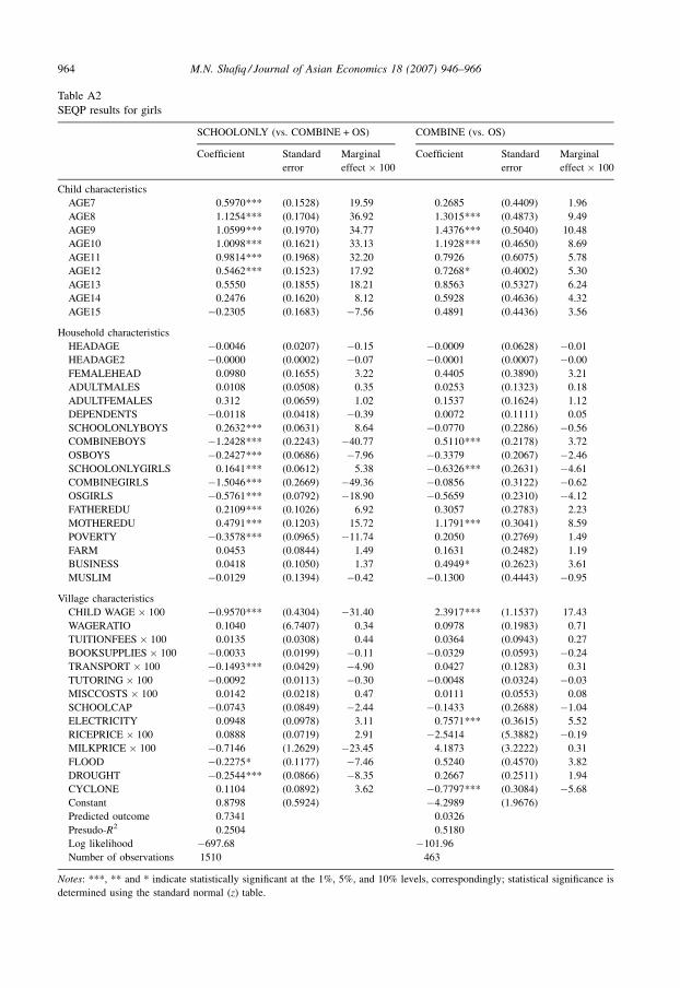
The SEQP results for boys and girls are shown in Appendix Tables 1 and 2. A comparison

between the MNL and SEQP specifications is possible for the marginal effects and standard

errors for COMBINE categories. This exercise provides evidence that results and conclusions

are sensitive to the choice of specification. The magnitudes of the marginal effects in the

SEQP are consistently larger than the MNL marginal effects. An exercise in constructing

confidence intervals for marginal effects of the statistically significant coefficients (not shown

in this paper) reveals that SEQP estimates do not lie in the 95% interval around the MNL

marginal effects, and vice versa. In addition, the MNL and SEQP specifications results are

somewhat different with respect to the statistical significance of coefficients: for boys, the

results vary for the number of adult males, number of dependents, and the price of rice; for

girls, the results differ for other OS girls, business-ownership, and flood occurrences. Overall,

unlike some other research comparing alternative specifications of household schooling and

child labor decisions (e.g., Grootaert, 1999a), this study cannot provide basis for favoring one

specification over another.

5.12. Limitations of the study

There are at least three limitations with the empirical analysis in this study. First, the small

proportion of boys and girls in COMBINE in the HIES 2000 arguably makes it redundant to

include the COMBINE category in the analysis, and that a category for schooling (i.e.,

SCHOOLONLY plus COMBINE) versus non-schooling (i.e., OS) is adequate. However, the

inclusion of COMBINE is warranted on the grounds of policy formulation: historical experiences

from today’s developed economies has shown that it takes much longer for policy to shift OS

children into SCHOOLONLY, than it does to shift OS children into COMBINE (Humphries,

2003). Unless there are substantial positive shocks, households gradually reduce child labor

practices (often over generations). Moreover, considering COMBINE in the study clarifies that

while the wealth paradox is correct in predicting that asset-ownership is positively associated

with household child labor practices, there is no paradox when it comes to asset-ownership and

school enrollment (i.e., asset-ownership is positively associated with schooling) in the case of

rural Bangladeshi households.

Second, data limitations prevent this and other similar studies from considering several

important determinants of household child activity decisions. These include variables

identifying extended families (who provide valuable support during hardship, thereby

alleviating the need for children to work), and the household’s perceived rate of return to

schooling. In studies from neighboring India, Kochar (2004) and Chamarbagwala (in press) find

that regional rates of return to schooling affect the schooling and child labor decisions of rural

households. I am unable to follow their approach because Bangladesh’s small size and

geographic mobility imply that rural households observe national labor market conditions; since

all households across regions would observe the same returns, it is redundant to follow Kochar

and Chamarbagwala.


Third, the usual endogeneity-related limitations of household-level empirical methods are

present and therefore undermine claims of causal relationships. Specifically, simultaneity bias

causes endogeneity issues: household expenditures reflect household income, which are affected

by labor supply decisions of parents, which in turn depend on whether or not children are in

school. Parental education and asset-ownership also create endogeneity-related problems

because each also determines poverty. Despite my use of dummy variables for poverty, parental

education, and asset-ownership, these simultaneity biases are likely to persist. There is also

possible omitted variable bias because of within-household differences between children.

Without unusually detailed data, it is not possible to completely correct for simultaneity and

omitted variable endogeneity issues and establish causal relationships. Therefore, the estimates

in this study provide suggestive evidence between a household’s decision and various

characteristics (at the child, household, and village-levels), but not necessarily definitive proof of

causal relationships.

6. Conclusion

This study used recent theoretical advances and empirical techniques to understand household

schooling and child labor decisions towards children in rural Bangladesh. In this concluding

section, I review the results and discuss the implications on educational and child labor policies.

The results indicate that household poverty is strongly associated with keeping children out of

school and practicing child labor. While education policymakers cannot eradicate poverty, the

results support the continued targeting of interventions at children from households living at or

below the poverty line in rural Bangladesh. For child labor policymakers, this result implies that

the current ban on child labor may be making survival difficult for poor households (since poor

households are dependent on the contributions of their children).

The results suggest that households with educated parents have a deep appreciation for

schooling and distaste for child labor. Under an inter-generational ceteris paribus assumption,

the results imply that educating the present generation may increase school enrolment and reduce

child labor in the next generation. For educational policy, the results suggest targeting

interventions towards children from households where one or more of the parents have not

completed primary education.

There is a positive association between household ownership of assets (such as farm, land, or

business) and sending children to school. In some cases, however, asset-owning households may

also decide to have the child combine schooling with child labor. Thus, initiatives that support

asset-ownership (such as microfinance initiatives) may be contributing to greater school

enrolment, but may not be reducing child labor; a caveat is that initiatives that encourage

household asset-ownership may improve the nature of work for some children (since a child is

arguably better off working for her own household rather than an outside employer). In terms of

educational policy, the results support targeting interventions at children from households

without assets.

Regarding intra-household decisions, the results indicate that households in rural Bangladesh

prefer to make the same decision for all children within the household, regardless of gender.

Moreover, I find no evidence of the household sacrificing girl’s schooling for boys’ schooling.

The educational policy implication, therefore, is that interventions in rural Bangladesh should

target both boys and girls.

The results suggest small associations between some direct costs of schooling and household

decisions: when facing high transportation costs, girls are likely to combine schooling with child


labor; and, greater private tutoring costs dissuade the household from enrolling boys in school.

The coefficients for tuition, fees, books, supplies and uniform are not statistically significant.

This lack of statistical association, however, does not necessarily imply that households are not

sensitive to most direct costs, and that policymakers should raise direct costs. Rather, is the issue

of user-fees in education is a sensitive political issue in rural Bangladesh and should be carefully

addressed through in-depth research on direct cost items. For example, future research can

examine the willingness of households to pay for nearer schools, and investigate the main

determinants of household expenditure on private tutoring (e.g., teacher absenteeism and low

school quality; Bray, 1999; Chaudhury, Hammer, Kremer, Muralidharan, & Rogers, 2006). For

now, the results suggest that educational policy in rural Bangladesh should address school

building or transportation initiatives for girls and affordable tutoring alternative for boys.

Finally, the results indicate that rural Bangladeshi households are sensitive to the indirect cost

of schooling. I find that households in villages with better child wages are more likely to send

children to school, but are hesitant to give up child labor earnings and instead have children

combine schooling with child labor. Since these indirect costs are substantial in rural Bangladesh,

a policy involving full-compensation to out-of-school children for indirect costs is prohibitively

costly; however, Mexico’s Opportunidades program (formerly Progresa) provides guidance on

how a well-designed conditional cash transfer program can offer partial compensation and still

succeed in increasing school enrollment and reducing child labor practices among rural

households (Schultz, 2004).10

Acknowledgements

I have benefited from seminars at the Annual Meetings of the Southern Economic Association

(2005), Annual Meetings of the Comparative International Education Society (2004), World

Bank Resident Mission in Dhaka, Columbia University, Florida State University, and

Washington and Lee University. For helpful comments and discussions, I am deeply appreciative

to Christine Allison, Mary Arends-Kuenning, Amita Chudgar, Kevin Dougherty, M. Shahe

Emran, Kristi Fair, Zahid Hussain, Nancy Kendall, Milagros Nores, Francisco Rivera-Batiz,

Nazia Shafiq, Miguel Urquiola, Salman Zaidi (for providing the data), and especially Henry M.

Levin, Amit Dar, Harry Patrinos, Mun Tsang, and an anonymous referee. This study is a part of

my doctoral dissertation, and largely conducted during appointments at the National Center for

Study of Privatization in Education (Teachers College, Columbia University) and World Bank

Resident Mission in Dhaka; their financial support and kind hospitality are gratefully

acknowledged. I alone am responsible for all findings, views, and errors.

Appendix A

Tables A1 and A2.


10 If the government were to compensate the 4.8 million out-of-school children (in the 5–14 age-group; Bangladesh

Bureau of Statistics, 2003) at the average daily wage rate of US$ 0.67 (Tk. 34.10) per day (as reported in the HIES 2000),

it would cost the government US$ 96.28 million per month (Tk. 4.91 billion per month), or US$ 962.82 million for the

school year (Tk. 49.10 billion per year), in addition to various administrative and monitoring costs; furthermore, there are

costs of providing additional schools, supplies, and staff. This translates to at least doubling of the Government of

Bangladesh’s total annual educational expenditures (for Bangladesh’s public expenditure review, see World Bank and

Asian Development Bank, 2003b).


Table A1

SEQP results for boys

SCHOOLONLY (vs. COMBINE + OS) COMBINE (vs. OS)


error

Marginal

effect � 100


error

Marginal

effect � 100


AGE7 0.2785*** (0.1262) 10.52 0.7647* (0.4244) 4.19

AGE8 0.8014*** (0.1352) 30.27 1.1812*** (0.4566) 6.48

AGE9 1.0693*** (0.1540) 40.39 1.1895*** (0.5104) 6.52

AGE10 0.6444*** (0.1244) 24.34 1.4780*** (0.4270) 8.11

AGE11 0.6183*** (0.1514) 23.35 1.1411*** (0.4872) 6.26

AGE12 0.2388* (0.1238) 9.02 0.5897 (0.4478) 3.23

AGE13 �0.1412 (0.1440) �5.33 1.1416*** (0.4386) 6.36

AGE14 �0.2982*** (0.1384) �11.27 0.7101 (0.4443) 3.89

AGE15 �0.6666*** (0.1354) �25.18 0.3271 (0.4280) 1.79


HEADAGE �0.0121 (0.0173) �0.46 �0.0029 (0.0467) �0.02

HEADAGE2 0.0001* (0.0002) 0.00 0.0001*(0 (0.0005) 0.00

FEMALEHEAD �0.2491 (0.1449) �9.41 0.1727 (0.3304) 0.95

ADULTMALES �0.0070 (0.0403) �0.27 �0.1821* (0.1021) �1.00

ADULTFEMALES 0.0597 (0.0546) 2.25 0.1406 (0.1254) 0.77

DEPENDENTS �0.0332 (0.0314) �1.25 0.1359* (0.0819) 0.75

SCHOOLONLYBOYS 0.0973* (0.0504) 3.68 �0.0654 (0.1394) �0.36

COMBINEBOYS �0.8965*** (0.1799) �33.86 0.5803*** (0.2125) 3.18

OSBOYS �0.4082*** (0.0514) �15.42 �0.2720* (0.1531) �1.49


COMBINEGIRLS �1.0115*** (0.1761) �38.21 1.3704*** (0.2348) 7.52

OSGIRLS �0.2499*** (0.0642) �9.44 �0.1277 (0.1648) �0.70

FATHEREDU 0.3113*** (0.0818) 11.76 0.5927*** (0.2011) 3.25

MOTHEREDU 0.3208*** (0.0955) 12.18 0.6525*** (0.2255) 3.58

POVERTY �0.2469*** (0.7290) �9.44 �0.5378*** (0.2029) �2.95

FARM 0.3236*** (0.0653) 11.76 0.2997* (0.1799) 1.64

BUSINESS �0.0256 (0.0744) 12.12 0.2008 (0.1782) 1.10

MUSLIM �0.2322** (0.1173) �9.32 0.1045 ((0.3401)) 0.57


CHILDWAGE � 100 �0.4319 (0.3648) �16.32 1.0168** (0.9478) 5.58

WAGERATIO 0.0170 (0.0509) 0.64 0.2204 (0.1452) 1.21

TUITIONFEES � 100 �0.0174 (0.0300) �0.66 0.0892 (0.0844) 0.49

BOOKSUPPLIES � 100 0.0077 (0.0179) 0.29 0.0208 (0.0441) 0.11

TRANSPORT � 100 0.0044 (0.0228) 0.17 �0.0087 (0.0628) �0.05

TUTORING � 100 0.0076 (0.0094) 0.29 �0.0562* (0.0327) �0.31

MISCCOSTS � 100 �0.0200 (0.0245) �0.75 0.0989*** (0.0652) 0.54

SCHOOLCAP 0.0519 (0.0646) 1.96 �0.0985 (0.1859) �0.54

ELECTRICITY 0.1519*** (0.0689) 5.74 0.2847 (0.1966) 1.56

RICEPRICE � 100 0.0527 (0.0690) 6.9 �6.9275 (5.0471) �37.99

MILKPRICE � 100 �0.2302 (0.5876) �8.7 �4.3133* (2.4749) �23.66

FLOOD 0.0367 (0.0922) 1.4 �0.2039 (0.2350) �1.12

DROUGHT �0.0697 (0.0653) �2.63 �0.3162* (0.1830) �1.73

CYCLONE �0.0117 (0.0705) �0.44 �0.0198 (0.2175) �0.11

Constant 0.5177 (0.4925) �1.6286 (1.4461)


Presudo-R2 0.2193 0.5107

Log likelihood �1165.40 �171.08

Number of observations 2229 874




Table A2

SEQP results for girls

SCHOOLONLY (vs. COMBINE + OS) COMBINE (vs. OS)


error

Marginal

effect � 100


error

Marginal

effect � 100


AGE7 0.5970*** (0.1528) 19.59 0.2685 (0.4409) 1.96

AGE8 1.1254*** (0.1704) 36.92 1.3015*** (0.4873) 9.49

AGE9 1.0599*** (0.1970) 34.77 1.4376*** (0.5040) 10.48

AGE10 1.0098*** (0.1621) 33.13 1.1928*** (0.4650) 8.69

AGE11 0.9814*** (0.1968) 32.20 0.7926 (0.6075) 5.78

AGE12 0.5462*** (0.1523) 17.92 0.7268* (0.4002) 5.30

AGE13 0.5550 (0.1855) 18.21 0.8563 (0.5327) 6.24

AGE14 0.2476 (0.1620) 8.12 0.5928 (0.4636) 4.32

AGE15 �0.2305 (0.1683) �7.56 0.4891 (0.4436) 3.56


HEADAGE �0.0046 (0.0207) �0.15 �0.0009 (0.0628) �0.01

HEADAGE2 �0.0000 (0.0002) �0.07 �0.0001 (0.0007) �0.00

FEMALEHEAD 0.0980 (0.1655) 3.22 0.4405 (0.3890) 3.21

ADULTMALES 0.0108 (0.0508) 0.35 0.0253 (0.1323) 0.18

ADULTFEMALES 0.312 (0.0659) 1.02 0.1537 (0.1624) 1.12

DEPENDENTS �0.0118 (0.0418) �0.39 0.0072 (0.1111) 0.05

SCHOOLONLYBOYS 0.2632*** (0.0631) 8.64 �0.0770 (0.2286) �0.56

COMBINEBOYS �1.2428*** (0.2243) �40.77 0.5110*** (0.2178) 3.72

OSBOYS �0.2427*** (0.0686) �7.96 �0.3379 (0.2067) �2.46


COMBINEGIRLS �1.5046*** (0.2669) �49.36 �0.0856 (0.3122) �0.62

OSGIRLS �0.5761*** (0.0792) �18.90 �0.5659 (0.2310) �4.12

FATHEREDU 0.2109*** (0.1026) 6.92 0.3057 (0.2783) 2.23

MOTHEREDU 0.4791*** (0.1203) 15.72 1.1791*** (0.3041) 8.59

POVERTY �0.3578*** (0.0965) �11.74 0.2050 (0.2769) 1.49

FARM 0.0453 (0.0844) 1.49 0.1631 (0.2482) 1.19

BUSINESS 0.0418 (0.1050) 1.37 0.4949* (0.2623) 3.61

MUSLIM �0.0129 (0.1394) �0.42 �0.1300 (0.4443) �0.95


CHILD WAGE � 100 �0.9570*** (0.4304) �31.40 2.3917*** (1.1537) 17.43

WAGERATIO 0.1040 (6.7407) 0.34 0.0978 (0.1983) 0.71

TUITIONFEES � 100 0.0135 (0.0308) 0.44 0.0364 (0.0943) 0.27

BOOKSUPPLIES � 100 �0.0033 (0.0199) �0.11 �0.0329 (0.0593) �0.24

TRANSPORT � 100 �0.1493*** (0.0429) �4.90 0.0427 (0.1283) 0.31

TUTORING � 100 �0.0092 (0.0113) �0.30 �0.0048 (0.0324) �0.03

MISCCOSTS � 100 0.0142 (0.0218) 0.47 0.0111 (0.0553) 0.08

SCHOOLCAP �0.0743 (0.0849) �2.44 �0.1433 (0.2688) �1.04

ELECTRICITY 0.0948 (0.0978) 3.11 0.7571*** (0.3615) 5.52

RICEPRICE � 100 0.0888 (0.0719) 2.91 �2.5414 (5.3882) �0.19

MILKPRICE � 100 �0.7146 (1.2629) �23.45 4.1873 (3.2222) 0.31

FLOOD �0.2275* (0.1177) �7.46 0.5240 (0.4570) 3.82

DROUGHT �0.2544*** (0.0866) �8.35 0.2667 (0.2511) 1.94

CYCLONE 0.1104 (0.0892) 3.62 �0.7797*** (0.3084) �5.68

Constant 0.8798 (0.5924) �4.2989 (1.9676)


Presudo-R2 0.2504 0.5180

Log likelihood �697.68 �101.96

Number of observations 1510 463



References

Arends-Kuenning, M., & Amin, S. (2004). School incentive programs and children’s activities: The case of Bangladesh.

Comparative Education Review, 48(3), 295–317.

Asadullah, M. N. (2006). Returns to education in Bangladesh. Education Economics, 14(4), 453–468.

Asgharie, K. (1993). Statistics on child labor. Bulletin of Labor Statistics, 3.

Baland, J., & Robinson, J. (2000). Is child labor inefficient? Journal of Political Economy, 108(4), 663–679.

Bangladesh Bureau of Statistics (2003). Report on National Child Labor Survey 2002–2003. Dhaka: Bangladesh Bureau

of Statistics.

Basu, K. (1999). Child labor: Cause, consequence and cure, with remarks on International Labor Standards. Journal of

Economic Literature, 37(3), 1083–1119.

Basu, K., & Van, P. (1998). The economics of child labor. American Economic Review, 88(3), 412–427.

Becker, G. (1960). Demographic and economic change in developed countries. Princeton: Princeton University Press.

Becker, G., & Lewis, H. G. (1973). Interaction between quantity and quality of children. Journal of Political Economy,

81(2), S279–S288.

Becker, G., & Mulligan, C. (1997). The endogenous determination of time preference. Quarterly Journal of Economics,

112(3), 729–757.

Beegle, K., Dehejia, R., Gatti, R. (2004). Why should we care about child labor? The education, labor market, and health

consequences of child labor. Working paper 19980, National Bureau of Economic Research.

Behrman, J., & Stacey, N. (1997). The social benefits of education. Ann Arbor: University of Michigan Press.

Bhalotra, S., & Heady, C. (2003). Child farm labor: The wealth paradox. The World Bank Economic Review, 17(2),

197–227.

Bhatty, K. (1998). Educational deprivation in India: A survey of field investigations.. Economic and Political Weekly 33

1731–1740 and 1858–1869.

Biggeri, M., Guarcello, L., Lyon, S., Rosati, F. (2003). The puzzle of idle children: Neither in school nor performing

economic activities: Evidence from six countries. Working paper 6, Understanding Children’s Work Project.

Binder, M., & Scrogin, D. (1999). Labor force participation and household work of urban schoolchildren in Mexico:

Characteristics and consequences. Economic Development and Cultural Change, 48(1), 123–147.

Bray, M. (1999). The shadow education system: Private tutoring and its implications for planners. Fundamental of

education planning series 61, Paris: UNESCO.

Brown, D., Deardorff, A., Stern, R. (2002). The determinants of child labor: Theory and evidence. Discussion Paper 486,

School of Public Policy, University of Michigan.

Chamarbagwala, R. (in press). Regional returns to education, child labor, and schooling in India. Journal of Development

Studies.

Chaudhury, N., Hammer, J., Kremer, M., Muralidharan, K., & Rogers, F. H. (2006). Missing in action: Teacher and health

workers absence in developing countries. Journal of Economic Perspectives, 20(1), 91–116.

Dar, A., Blunch, N., Kim, B., Sasaki, M. (2002). Participation of children in schooling and labor activities: A review of

empirical studies. Social Protection discussion paper 0221, The World Bank.

Deininger, K. (2003). Does cost of schooling affect enrollment by the poor? Universal primary education in Uganda.

Economics of Education Review, 22(3), 291–305.

Dreze, J., & Kingdon, G. (2001). School participation in rural India. Review of Development Economics, 5(1), 1–24.

Duryea, S., & Arends-Kuenning, M. (2003). School attendance, child labor and local labor market fluctuations in urban

Brazil. World Development, 31(7), 1165–1178.

Edmonds, E. (2005). Does child labor decline with improving economic status? Journal of Human Resources, 40(1),

77–99.

Edmonds, E. (2007). Child labor. In J. Strauss & T. P. Schultz (Eds.), The Handbook of Development Economics (Vol. 4),

Amsterdam: North Holland.

Edmonds, E., & Pavcnik, N. (2005). Child labor in the global economy. Journal of Economic Perspectives, 19(1), 199–

220.

Edmonds, E., & Turk, C. (2004). Child labor in transition in Vietnam. In P. Glewwe, N. Agrawal, & D. Dollar (Eds.),

Economic growth, poverty and household welfare in Vietnam (pp. 505–550). Washington, DC: World Bank.

Glewwe, P. (2002). Schools and skills in developing countries: Educational policies and socioeconomic outcomes.

Journal of Economic Literature, 40(2), 436–482.

Grootaert, C. (1999a). Child labor in Cote d’Ivoire. In C. Grootaert & H. Patrinos (Eds.), The policy analysis of child

labor: A comparative study (pp. 23–62). New York: St. Martins Press.


Grootaert, C. (1999b). Modeling the determinants. In C. Grootaert & H. Patrinos (Eds.), The policy analysis of child labor:

A comparative study (pp. 13–22). New York: St. Martins Press.

Grootaert, C., & Patrinos, H. (1999). The policy analysis of child labor: A comparative study. New York: St Martin’s Press.

Hannum, E., & Buchmann, C. (2004). Global educational expansion and socio-economic development: An assessment of

findings from the social sciences. World Development, 33(3), 333–354.

Hausman, J., & McFadden, D. (1984). Specification tests for the multinomial logit. Econometrica, 52(5), 1219–1240.

Hazarika, G. (2001). The sensitivity of primary school enrollment to the costs of post-primary schooling in rural Pakistan:

A gender perspective. Education Economics, 10(2), 237–244.

Holmes, J. (2003). Measuring the determinants of school completion in Pakistan: Analysis of censoring and selection bias.

Economics of Education Review, 22(3), 249–264.

Humphries, J. (2003). Child labor: Lessons from the historical experience of today’s industrial economies. The World

Bank Economic Review, 17(2), 175–196.

Kochar, A. (2004). Urban Influences on Rural Schooling in India. Journal of Development Economics, 74(1), 113–136.

Ljungqvist, L. (1993). Economic underdevelopment: The case of a missing market for human capital. Journal of

Development Economics, 40(2), 219–239.

Long, J., & Freese, J. (2006). Regression models for categorical dependent variables using Stata (2nd ed.). College

Station, Texas: Stata Press.

Loury, G. (1981). Intergenerational transfers and the distribution of earnings. Econometrica, 49(4), 843–867.

Maddala, G. S. (1983). Limited-dependent and qualitative variables in econometrics. New York: Cambridge University

Press.

Maitra, P. (2003). Schooling and educational achievement: Evidence from Bangladesh. Education Economics, 11(2),

129–153.

Maitra, P., & Ray, R. (2002). The joint estimation of child participation in schooling and employment: Comparative

evidence from three continents. Oxford Development Studies, 30(1), 41–62.

Morduch, J. (1999). The microfinance promise. Journal of Economic Literature, 37(4), 1569–1614.

O’Donnell, O., van Doorslaer, E., Rosati, F. (2002). Child labor and health: Evidence and research issues. Working paper

number 1, Understanding Children’s Work Project.

Ranjan, P. (2001). Credit constraints and the phenomenon of child labor. Journal of Development Economics, 64(1), 81–

102.

Rossi, M., & Rosati, F. (2003). Children’s working hours and school enrolment: Evidence from Pakistan and Nicaragua.

The World Bank Economic Review, 17(2), 283–295.

Rozenzweig, M., & Evenson, R. (1977). Fertility, schooling, and the economic contribution of children in rural India: An

econometric analysis. Econometrica, 45(5), 1065–1079.

Sander, W. (1995). Schooling and smoking. Economics of Education Review, 14(1), 22–33.

Schultz, T. W. (1960). Capital formation by education. Journal of Political Economy, 68(6), 571–583.

Schultz, T. P. (2004). School subsidies for the poor: Evaluating the Mexican Progresa poverty program. Journal of

Development Economics, 74(1), 199–250.

Strauss, J., & Thomas, D. (1995). Human resources: Empirical modeling of household and family decisions. In

Srinivasan, T. N., & Behrman, J. Eds. Handbook of development economics. Vol. 3A (pp.1885–2023). Amster-

dam: North Holland Press.Swaminathan, M. (1998). Economic growth and the persistence of child labor: Evidence from an Indian city. World

Development, 26(8), 523–1528.

Tsang, M. (1994). Private and public costs of schooling in developing nations. In T. Husen & T. Neville Postlethwaite

(Eds.), International encyclopedia of education (2nd ed., pp. 4702–4708). New York: Pergamon Press.

UNESCO, 2005. Education for All 2006: Global monitoring report 2006. Paris: UNESCO.

Udry, C. (2006). Child labor. In A. Banerjee, R. Benabou, & D. Mookherjee (Eds.), Understanding poverty. New York:

Oxford University Press.

World Bank. (2000). Bangladesh education sector review. Dhaka: The University Press Limited.

World Bank and Asian Development Bank (2003a). Poverty in Bangladesh: Building on progress. Joint report, The World

Bank and Asian Development Bank.

World Bank and Asian Development Bank, (2003b). Bangladesh: Public Expenditure Review. Joint report, The World

Bank and Asian Development Bank.

Wydick, B. (1999). The effect of microenterprise lending on child schooling in Guatemala. Economic Development and

Cultural Change, 47(4), 853–868.


Documents

Household schooling and child labor decisions in rural ...mnshafiq/M_Najeeb_Shafiq_(University_of_Pittsburgh... · Household schooling and child labor decisions in rural Bangladesh