Embed Size (px)
Citation preview

WP/08/211
House Price Developments in Europe: A Comparison
Paul Hilbers, Alexander W. Hoffmaister,
Angana Banerji, and Haiyan Shi

© 2008 International Monetary Fund WP/08/211 IMF Working Paper European Department
House Price Developments in Europe: A Comparison
Prepared by Paul Hilbers, Alexander W. Hoffmaister, Angana Banerji, and Haiyan Shi1
October 2008
Abstract
This Working Paper should not be reported as representing the views of the IMF. The views expressed in this Working Paper are those of the author(s) and do not necessarily represent those of the IMF or IMF policy. Working Papers describe research in progress by the author(s) and are published to elicit comments and to further debate.
House prices in Europe have shown diverging trends, and this paper seeks to explain these differences by analyzing three groups of countries: the “fast lane”, the average performers, and the slow movers. Price movements in the first two groups are found to be driven mostly by income and trends in user costs, and housing markets in these countries seem relatively more susceptible to adverse developments in fundamentals. Real house price declines among the slow movers are harder to explain, although ample supply, low home ownership, and less complete mortgage markets are likely factors. The impact of macroeconomic, prudential and structural policies on housing markets can be large and should be a factor in policy decisions. JEL Classification Numbers: R21, R31, G21 Keywords: Housing markets, Europe Authors’ E-Mail Addresses: [email protected], [email protected], [email protected],
1 The authors thank Martin Cihak, Stijn Claessens, James Daniel, Igan Deniz, Luc Everaert, Lorenzo Figliuoli, Simon Gray, Alessandro Leipold, and Ashok Mody for their useful comments. The paper also benefited from feedback from participants in a European Department seminar. Cristina Cheptea put together an extensive database and provided excellent research assistance. The authors are responsible for any remaining errors.

2
Contents Page
I. Introduction………........................................................................................................4 II. Understanding Market Developments ...........................................................................5 A. Key Features ............................................................................................................5 B. Determining Factors and Indicators.........................................................................7 C. Impact of Policies ....................................................................................................9 III. The European Picture: House Price Developments in Selected Countries..................12 A. Market Developments............................................................................................12 B. Demand Factors .....................................................................................................14 C. Supply Side and Rental Market .............................................................................22 D. Taxation Issues.......................................................................................................26 E. Financial Sector .....................................................................................................32
IV. Assessing House Price Developments: An Empirical Approach ................................35 A. House Price Model.................................................................................................35 B. Empirical Evidence................................................................................................40 V. Summary and Concluding Remarks ............................................................................50
References................................................................................................................................52 Boxes 1. Aspects of Housing Markets..........................................................................................6 2. User Cost Framework ....................................................................................................8 3. Measuring User Costs in Europe .................................................................................19 4. Do Housing Prices Reflect a Bubble?..........................................................................39 Tables 1. Indicators for Housing Market Conditions and Trends ...............................................10 2. Real House Price Index................................................................................................13 3. Evolution of User Costs in Europe, 1995–2006 ..........................................................18 4. Understanding the Decline in User Costs in Europe, 2000–05 ...................................18 5. Home Ownership in Europe.........................................................................................20 6. Housing Stocks ............................................................................................................22 7. Housing Stock Rented from Government and Social Housing ...................................25 8. Property-Related Taxes................................................................................................27 9. Mortgage Market Completeness Indicators .................................................................34 10. Standard Model Estimates for P/Rent..........................................................................40

3
11. Standard Model Estimates for P ..................................................................................41 12. User Costs and Interest Rates ......................................................................................42 13. Extended Model Estimates ..........................................................................................45 14. The Impact of the Risk-Free Interest Rate on User Costs ...........................................47 15. Overvaluation Resulting from an Increase in Interest Rates .......................................48 Figures 1. Key Policy Relationships.............................................................................................11 2. Average Real Property Prices, 1985–2007 ..................................................................13 3. House Prices and Income, 1985–2006.........................................................................15 4. House Prices and Interest Rates, 1985–2006...............................................................16 5. Demographics, 1985–2006 ..........................................................................................17 6. Home Ownership and Property Price Appreciation.....................................................21 7. Housing and Household Wealth ..................................................................................21 8. House Prices and Housing Supply, 1985–2006...........................................................23 9. House Prices and Rents, 1985–2006............................................................................25 10. Price-Rental Ratio and Housing Stock ........................................................................26 11. Selected European Countries: Property Taxes by Level, 1975–2005..........................29 12. Selected European Countries: Property Tax Change, 1975–2005...............................30 13. Selected European Countries: Property Tax Deflated by House Prices, 1975–2005 ..31 14. Financial Sector Lending for Residential Property, 1990–2004..................................33 15. Mortgage Lending Growth and Property Prices ..........................................................33 16. Understanding the House Price-Rental Ratio ..............................................................43 17. Understanding the House Price....................................................................................44 18. Overvaluation in Housing Markets in Europe .............................................................49 Appendices I. Data Sources ................................................................................................................55 II. Housing-Related Taxation ...........................................................................................56
4
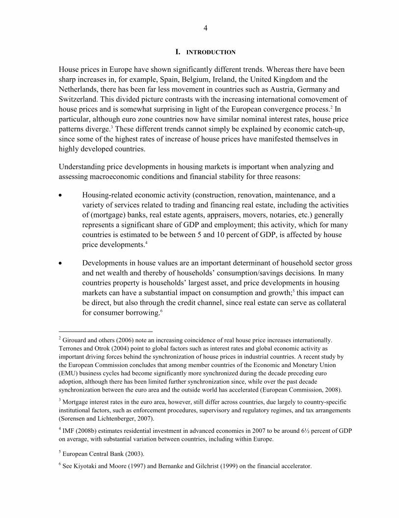
I. INTRODUCTION
House prices in Europe have shown significantly different trends. Whereas there have been sharp increases in, for example, Spain, Belgium, Ireland, the United Kingdom and the Netherlands, there has been far less movement in countries such as Austria, Germany and Switzerland. This divided picture contrasts with the increasing international comovement of house prices and is somewhat surprising in light of the European convergence process.2 In particular, although euro zone countries now have similar nominal interest rates, house price patterns diverge.3 These different trends cannot simply be explained by economic catch-up, since some of the highest rates of increase of house prices have manifested themselves in highly developed countries.
Understanding price developments in housing markets is important when analyzing and assessing macroeconomic conditions and financial stability for three reasons:
• Housing-related economic activity (construction, renovation, maintenance, and a variety of services related to trading and financing real estate, including the activities of (mortgage) banks, real estate agents, appraisers, movers, notaries, etc.) generally represents a significant share of GDP and employment; this activity, which for many countries is estimated to be between 5 and 10 percent of GDP, is affected by house price developments.4
• Developments in house values are an important determinant of household sector gross and net wealth and thereby of households’ consumption/savings decisions. In many countries property is households’ largest asset, and price developments in housing markets can have a substantial impact on consumption and growth;5 this impact can be direct, but also through the credit channel, since real estate can serve as collateral for consumer borrowing.6
2 Girouard and others (2006) note an increasing coincidence of real house price increases internationally. Terrones and Otrok (2004) point to global factors such as interest rates and global economic activity as important driving forces behind the synchronization of house prices in industrial countries. A recent study by the European Commission concludes that among member countries of the Economic and Monetary Union (EMU) business cycles had become significantly more synchronized during the decade preceding euro adoption, although there has been limited further synchronization since, while over the past decade synchronization between the euro area and the outside world has accelerated (European Commission, 2008). 3 Mortgage interest rates in the euro area, however, still differ across countries, due largely to country-specific institutional factors, such as enforcement procedures, supervisory and regulatory regimes, and tax arrangements (Sorensen and Lichtenberger, 2007). 4 IMF (2008b) estimates residential investment in advanced economies in 2007 to be around 6½ percent of GDP on average, with substantial variation between countries, including within Europe.
5 European Central Bank (2003). 6 See Kiyotaki and Moore (1997) and Bernanke and Gilchrist (1999) on the financial accelerator.
5
• House prices, if out of line with fundamentals, can be a threat to economic and financial stability. A better understanding of the process that determines house prices allows an informed assessment of potential overvaluation in the market, which can become a source of economic and financial instability.7
This study aims at determining the main factors behind the divergence in house price developments in Europe. Section II discusses the key features of housing markets that set these markets apart from durable goods and financial asset markets and that are key to interpreting price developments; it provides guidance on how to assess housing market developments and discusses the various relevant indicators. Section III presents selected stylized facts, focusing on key determining factors, and an effort is undertaken to measure user costs, a major factor in understanding house price developments.8 Section IV estimates real house price equations, including income, user costs, demographic developments, and other variables discussed in earlier sections as explanatory variables. In contrast to other housing studies,9 this paper does not focus on deriving a relationship for individual countries, but on trying to uncover differences between three distinct groups of European countries: those with until recently very rapidly increasing house prices (the “fast lane”), those showing a closer to average development (the “average performers”), and those with relatively stagnant house prices (the “slow movers”). Section V concludes.
II. UNDERSTANDING MARKET DEVELOPMENTS
A. Key Features
Houses have a number of unusual features that complicate the interpretation of price developments. The key differences with other products purchased by households, including consumer durables, are summarized in Box 1. In particular, the heterogeneity of the product—no two houses are fully alike—and the low turnover of individual houses complicate the determination and interpretation of average price developments.10 For instance, increases in the mean or median price index can indicate that prices of comparable houses are increasing, but also reflect improvements in the quality of the stock (e.g., due to renovations and expansions)11 or quicker turnover of houses at the high end of the market. In addition, there may also be large regional differences in house price developments, which are
7 Collyns and Senhadji (2002). 8 The analysis generally covers the period up to 2007 and is carried out for a group of 16 advanced European countries for which reliable long-term housing data could be compiled: Austria, Belgium, Denmark, Finland, France, Germany, Greece, Ireland, Italy, the Netherlands, Norway, Portugal, Spain, Sweden, Switzerland, and the United Kingdom. 9 See e.g. Girouard and others (2006) and IMF (2008b). 10 See Bank for International Settlements (2005) for details. 11 Expansions, it can be argued, increase the quantity rather than quality of housing, which could be corrected for by measuring house prices in terms of square footage.

6
Box 1. Aspects of Housing Markets Key features Housing markets are different from most other markets, both in terms of the product and the transaction process. Important features are:
• heterogeneity: different properties have different characteristics, and even for identical properties the location—a key factor in the price—will differ;
• high transaction costs and low turnover: transaction costs are often high and trades in a particular property are usually infrequent, which hampers assessing price developments;
• varying conditions of sales: prices generally result from bilateral negotiations, which include agreements on the price, but also on the condition of the property (e.g., “as is” as opposed to after certain repairs/renovations) and other aspects of the sale (timing, distribution of costs);
• rigid supply: supply may lag demand as a result of scarcity of buildable land and, even if land is widely available, the time needed to secure building permits, obtain financing, and finish construction; in case of a sudden slowdown in demand, the supply response will also be lagged;
• varying financing conditions: these vary widely internationally; key factors include the presence of specialized mortgage finance institutions and mortgage-backed securities markets, options to refinance and the use of real estate as collateral, and the supervisory and regulatory framework for housing finance;
• impact of taxes and subsidies: taxation of, and financial incentives for, home ownership can strongly affect conditions in housing markets; examples include real estate taxes, the tax deductibility of certain costs (such as mortgage interest payments), and housing subsidies.
Measurement issues The key challenge in measuring real estate developments is the comparability of the objects. Often, price developments are measured by monitoring the mean or median of all transaction prices observed. This information is relatively easy to collect, but may suffer from shifts in the composition of objects that change owner. This drawback is avoided by focusing on one sort of well-defined property that can be considered representative for the market. Alternatively, the repeat sales method (used, e.g., for the Standard and Poor’s Case-Shiller index in the United States) focuses on transactions in a single property, but requires at least two sales, and does not account for possible changes in the quality of the object over time. Hedonic price models correct for quality changes through econometric techniques; they are generally the preferred option, but require large and detailed data sets and may suffer from bias due to incorrect model specification.
Data availability Real estate markets are among the less transparent asset markets. The lack of good quality and timely data on real estate developments is a major complicating factor in assessing whether these developments are a cause for concern or not. Available cross-country databases generally do not include key data necessary to assess conditions in real estate markets, such as price indices and data on rents, vacancy rates, construction costs, real estate lending, etc. A frequently used source, also for this study, is the database compiled by the Bank for International Settlements (BIS), which includes a selection of annual and quarterly data for property markets in selected industrial and emerging market countries, based on official and private sources. In addition, we make use of the Hypostat database put together by the European Mortgage Federation (EMF, 2006a).
Sources: Bank for International Settlements (2005); Hilbers, Lei, and Zacho (2001).

7
not captured by nationwide averages, but are likely to have economic and financial implications that are different from those under a more uniform distribution. More generally, houses are nontradables, which—except to some extent for second (vacation) homes and investment properties—limits international arbitrage.
In addition, there is no unified data set for Europe. Many national data-collecting agencies—including statistical offices and central banks—compile housing data, but the coverage and definitions vary widely. Some data are derived wholly or partly from private sources, which may not cover the complete market. Available time series are often short. Moreover, for Eastern Europe data limitations are more severe, and available time series often cover only a limited period and/or only a subset of dwellings (e.g., high-end apartments and housing in the capital); these countries are not included in this study.12
B. Determining Factors and Indicators
Key determining factors include disposable income and interest rates. Interest rates play a dual role: mortgage rates determine financing costs, while the risk-free interest rate serves as an indicator of opportunity costs. The total debt service on a mortgage as a share of disposable income is often used as a measure for the “affordability” of the housing stock.13 Other important demand factors include demographics, specifically population growth and developments in the number and size of households. Since renting (renting out) is an alternative to buying (selling) a home, developments and conditions in the rental market affect those in the housing market.
The user cost framework combines various factors that impinge on house prices. This framework is based on the premise that, in the long run, the expected costs of home ownership—the user costs—should equal those of renting (Poterba, 1984). Key user cost elements include mortgage interest costs (corrected for possible tax deductibility), maintenance costs, property taxes, and expected net capital gains (Box 2).
An important element in determining user costs is taxation. Housing is subject to a variety of taxes, generally linked to ownership and transactions. Examples of the former include real estate taxes and taxation of (imputed) rents, while transaction taxes include turnover taxes and local and regional levies for transferring ownership. In addition, there can be (implicit) subsidies involved in renting or owning, including through the tax deductibility of mortgage interest and the tax treatment of capital gains.
12 See European Central Bank (2007a) and Egert and Mihaljek (2007) for an analysis of recent developments in house prices in Central and Eastern Europe.
13 An analysis of household balance sheets can determine the indebtedness and interest sensitivity of households; see Allen and others (2002) and International Monetary Fund (2005). It can also help assess the implications of a decline in house prices on households’ solvency.
8
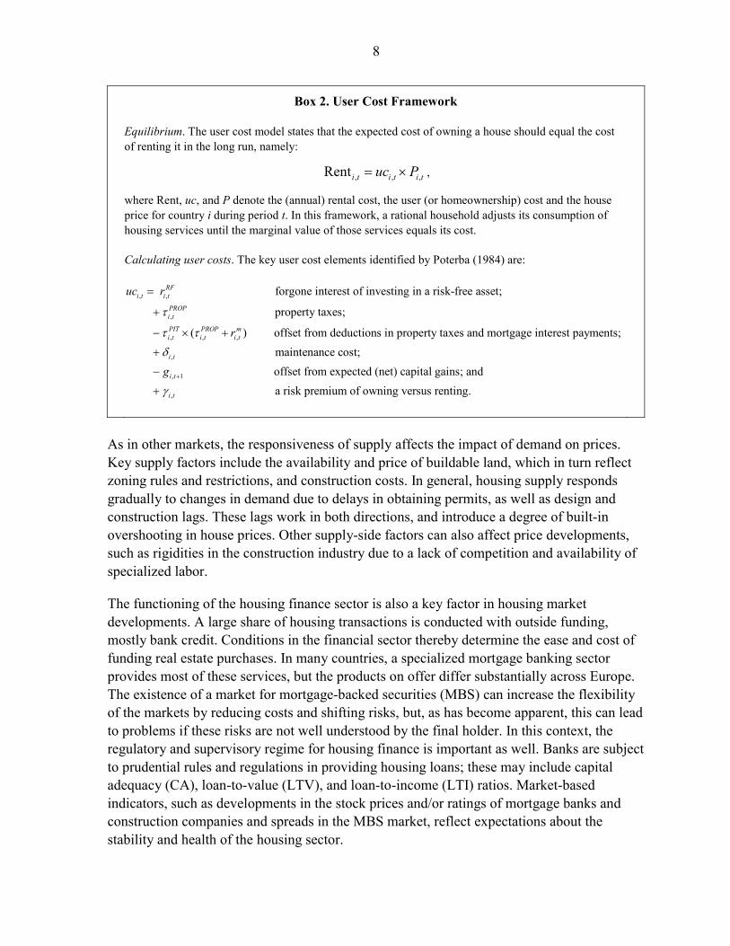
Box 2. User Cost Framework
Equilibrium. The user cost model states that the expected cost of owning a house should equal the cost of renting it in the long run, namely:
, , ,Rent i t i t i tuc P= × ,
where Rent, uc, and P denote the (annual) rental cost, the user (or homeownership) cost and the house price for country i during period t. In this framework, a rational household adjusts its consumption of housing services until the marginal value of those services equals its cost.
Calculating user costs. The key user cost elements identified by Poterba (1984) are:
, ,
,
, , ,
forgone interest of investing in a risk-free asset;
property taxes;
( ) offset from deduc
RFi t i t
PROPi t
PIT PROP mi t i t i t
uc r
r
τ
τ τ
=
+
− × +
,
, 1
,
tions in property taxes and mortgage interest payments; maintenance cost;
offset from expected (net) capital gains; and
i t
i t
i t
gδ
γ+
+
−
+ a risk premium of owning versus renting.
As in other markets, the responsiveness of supply affects the impact of demand on prices. Key supply factors include the availability and price of buildable land, which in turn reflect zoning rules and restrictions, and construction costs. In general, housing supply responds gradually to changes in demand due to delays in obtaining permits, as well as design and construction lags. These lags work in both directions, and introduce a degree of built-in overshooting in house prices. Other supply-side factors can also affect price developments, such as rigidities in the construction industry due to a lack of competition and availability of specialized labor.
The functioning of the housing finance sector is also a key factor in housing market developments. A large share of housing transactions is conducted with outside funding, mostly bank credit. Conditions in the financial sector thereby determine the ease and cost of funding real estate purchases. In many countries, a specialized mortgage banking sector provides most of these services, but the products on offer differ substantially across Europe. The existence of a market for mortgage-backed securities (MBS) can increase the flexibility of the markets by reducing costs and shifting risks, but, as has become apparent, this can lead to problems if these risks are not well understood by the final holder. In this context, the regulatory and supervisory regime for housing finance is important as well. Banks are subject to prudential rules and regulations in providing housing loans; these may include capital adequacy (CA), loan-to-value (LTV), and loan-to-income (LTI) ratios. Market-based indicators, such as developments in the stock prices and/or ratings of mortgage banks and construction companies and spreads in the MBS market, reflect expectations about the stability and health of the housing sector.

9
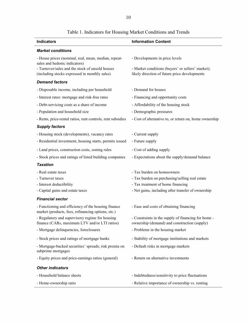
All in all, the qualitative information and the data set required for an in-depth analysis of house price developments is extensive. Table 1 describes the information content of the indicators relevant to assess price developments. Included are indicators on market conditions, demand and supply factors, taxation, financial sector conditions, and structural factors. A key challenge in deriving an overall view of the conditions in a housing market, for instance whether there is a risk of overvaluation or in order to make predictions about the direction of future price movements, is the need to combine this information. Solely basing an assessment on only one or a few variables or ratios—such as, for example, the house price to rents or to income ratio—may not do justice to the impact of other important determining factors, such as supply, rental market conditions, taxation and demographics. Nevertheless, a sharp rise in certain ratios, or historically high levels, should trigger a more detailed study of the underlying factors and possible risks to macroeconomic and financial stability.
Reliable and consistent data series for longer periods for many of these housing-related indicators are hard to collect, and the rest of this paper will focus on the subset of indicators for which there are good-quality and sufficiently long time-series data available.
C. Impact of Policies
Housing markets are affected by macroeconomic, prudential, and structural policies. These policies work through the various factors determining housing market conditions, as discussed above. Specifically,
• Monetary policy affects short-term interest rates, which either directly or through their impact on longer-term rates and inflationary expectations will have an important impact on house price developments. It influences both the demand and supply side of the housing market, the latter through the costs of borrowing for developers and builders.
• Fiscal policy affects house prices and their fundamentals via a host of taxes and subsidies. For example, disposable income is affected through (changes in) income taxation and the tax deductibility of certain costs; user costs include real estate taxation; subsidies can affect the relative cost of renting versus owning, as well as building activity (supply); and turnover taxes influence transaction costs.
• Supervisory and regulatory (prudential) policies affect house prices through their impact on the cost and ease of financing house purchases. These typically include capital requirements for lenders and loan limits for borrowers, but also the legal framework for the use of collateral (e.g., regulations on foreclosure and eviction).
• Structural policies, in particular labor market policies, competition policies, and land and zoning policies, affect construction costs and thereby the supply of housing.
10
Table 1. Indicators for Housing Market Conditions and Trends
Indicators Information Content
Market conditions
- House prices (nominal, real, mean, median, repeat-sales and hedonic indicators)
- Developments in price levels
- Turnover/sales and the stock of unsold houses (including stocks expressed in monthly sales)
- Market conditions (buyers’ or sellers’ market); likely direction of future price developments
Demand factors
- Disposable income, including per household - Demand for houses
- Interest rates: mortgage and risk-free rates - Financing and opportunity costs
- Debt-servicing costs as a share of income - Affordability of the housing stock
- Population and household size - Demographic pressures
- Rents, price-rental ratios, rent controls, rent subsidies - Cost of alternative to, or return on, home ownership
Supply factors
- Housing stock (developments), vacancy rates - Current supply
- Residential investment, housing starts, permits issued - Future supply
- Land prices, construction costs, zoning rules - Cost of adding supply
- Stock prices and ratings of listed building companies - Expectations about the supply/demand balance
Taxation
- Real estate taxes - Turnover taxes - Interest deductibility - Capital gains and estate taxes
- Tax burden on homeowners - Tax burden on purchasing/selling real estate - Tax treatment of home financing - Net gains, including after transfer of ownership
Financial sector
- Functioning and efficiency of the housing finance market (products, fees, refinancing options, etc.)
- Ease and costs of obtaining financing
- Regulatory and supervisory regime for housing finance (CARs, maximum LTV and/or LTI ratios)
- Constraints in the supply of financing for home - ownership (demand) and construction (supply)
- Mortgage delinquencies, foreclosures - Problems in the housing market
- Stock prices and ratings of mortgage banks - Stability of mortgage institutions and markets
- Mortgage-backed securities’ spreads; risk premia on subprime mortgages
- Default risks in mortgage markets
- Equity prices and price-earnings ratios (general) - Return on alternative investments
Other indicators
- Household balance sheets - Indebtedness/sensitivity to price fluctuations
- Home-ownership ratio - Relative importance of ownership vs. renting
11
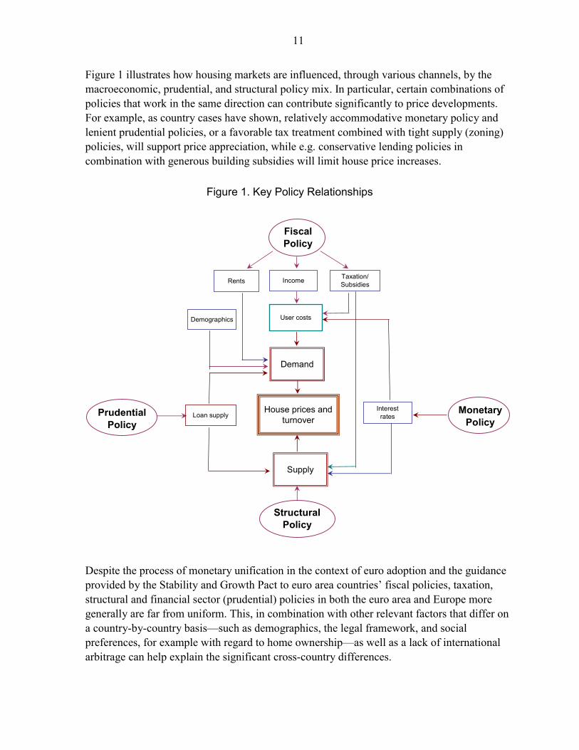
Figure 1 illustrates how housing markets are influenced, through various channels, by the macroeconomic, prudential, and structural policy mix. In particular, certain combinations of policies that work in the same direction can contribute significantly to price developments. For example, as country cases have shown, relatively accommodative monetary policy and lenient prudential policies, or a favorable tax treatment combined with tight supply (zoning) policies, will support price appreciation, while e.g. conservative lending policies in combination with generous building subsidies will limit house price increases.
Demand
House prices and turnover
Rents
User costs
Figure 1. Key Policy Relationships
Supply
Interest rates
Income
Prudential Policy
Fiscal Policy
Monetary Policy
Structural Policy
Taxation/Subsidies
Demographics
Loan supply
Despite the process of monetary unification in the context of euro adoption and the guidance provided by the Stability and Growth Pact to euro area countries’ fiscal policies, taxation, structural and financial sector (prudential) policies in both the euro area and Europe more generally are far from uniform. This, in combination with other relevant factors that differ on a country-by-country basis—such as demographics, the legal framework, and social preferences, for example with regard to home ownership—as well as a lack of international arbitrage can help explain the significant cross-country differences.
12
III. THE EUROPEAN PICTURE: HOUSE PRICE DEVELOPMENTS IN SELECTED COUNTRIES
A. Market Developments
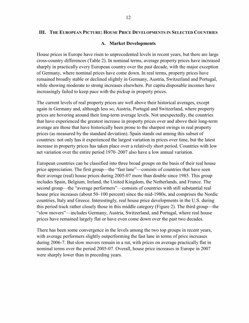
House prices in Europe have risen to unprecedented levels in recent years, but there are large cross-country differences (Table 2). In nominal terms, average property prices have increased sharply in practically every European country over the past decade, with the major exception of Germany, where nominal prices have come down. In real terms, property prices have remained broadly stable or declined slightly in Germany, Austria, Switzerland and Portugal, while showing moderate to strong increases elsewhere. Per capita disposable incomes have increasingly failed to keep pace with the pickup in property prices.
The current levels of real property prices are well above their historical averages, except again in Germany and, although less so, Austria, Portugal and Switzerland, where property prices are hovering around their long-term average levels. Not unexpectedly, the countries that have experienced the greatest increase in property prices over and above their long-term average are those that have historically been prone to the sharpest swings in real property prices (as measured by the standard deviation). Spain stands out among this subset of countries: not only has it experienced the largest variation in prices over time, but the latest increase in property prices has taken place over a relatively short period. Countries with low net variation over the entire period 1970–2007 also have a low annual variation.
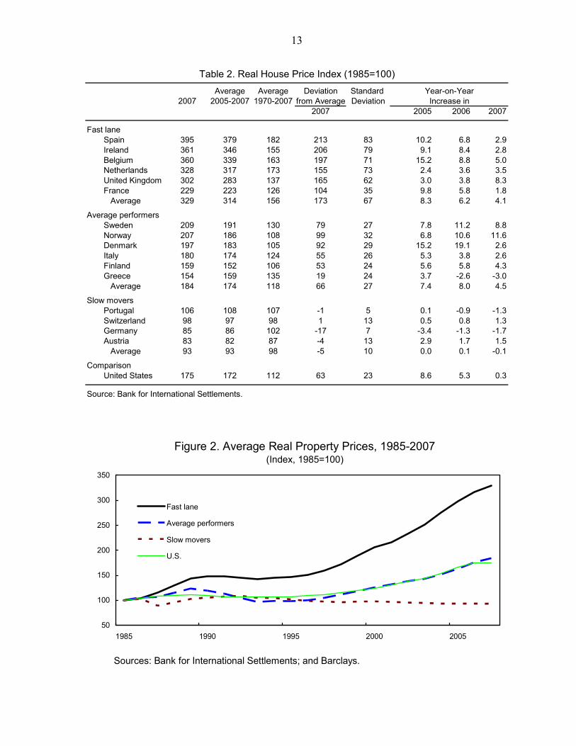
European countries can be classified into three broad groups on the basis of their real house price appreciation. The first group—the “fast lane”—consists of countries that have seen their average (real) house prices during 2005-07 more than double since 1985. This group includes Spain, Belgium, Ireland, the United Kingdom, the Netherlands, and France. The second group—the “average performers”—consists of countries with still substantial real house price increases (about 50–100 percent) since the mid-1980s, and comprises the Nordic countries, Italy and Greece. Interestingly, real house price developments in the U.S. during this period track rather closely those in this middle category (Figure 2). The third group—the “slow movers”—includes Germany, Austria, Switzerland, and Portugal, where real house prices have remained largely flat or have even come down over the past two decades.
There has been some convergence in the levels among the two top groups in recent years, with average performers slightly outperforming the fast lane in terms of price increases during 2006-7. But slow movers remain in a rut, with prices on average practically flat in nominal terms over the period 2005-07. Overall, house price increases in Europe in 2007 were sharply lower than in preceding years.
13
Average Average Deviation Standard 2007 2005-2007 1970-2007 from Average Deviation
2007 2005 2006 2007
Fast laneSpain 395 379 182 213 83 10.2 6.8 2.9Ireland 361 346 155 206 79 9.1 8.4 2.8Belgium 360 339 163 197 71 15.2 8.8 5.0Netherlands 328 317 173 155 73 2.4 3.6 3.5United Kingdom 302 283 137 165 62 3.0 3.8 8.3France 229 223 126 104 35 9.8 5.8 1.8
Average 329 314 156 173 67 8.3 6.2 4.1
Average performersSweden 209 191 130 79 27 7.8 11.2 8.8Norway 207 186 108 99 32 6.8 10.6 11.6Denmark 197 183 105 92 29 15.2 19.1 2.6Italy 180 174 124 55 26 5.3 3.8 2.6Finland 159 152 106 53 24 5.6 5.8 4.3Greece 154 159 135 19 24 3.7 -2.6 -3.0
Average 184 174 118 66 27 7.4 8.0 4.5
Slow moversPortugal 106 108 107 -1 5 0.1 -0.9 -1.3Switzerland 98 97 98 1 13 0.5 0.8 1.3Germany 85 86 102 -17 7 -3.4 -1.3 -1.7Austria 83 82 87 -4 13 2.9 1.7 1.5
Average 93 93 98 -5 10 0.0 0.1 -0.1
ComparisonUnited States 175 172 112 63 23 8.6 5.3 0.3
Source: Bank for International Settlements.
Year-on-YearIncrease in
Table 2. Real House Price Index (1985=100)
Sources: Bank for International Settlements; and Barclays.
50
100
150
200
250
300
350
1985 1990 1995 2000 2005
Fast lane
Average performers
Slow movers
U.S.
Figure 2. Average Real Property Prices, 1985-2007(Index, 1985=100)
14
B. Demand Factors
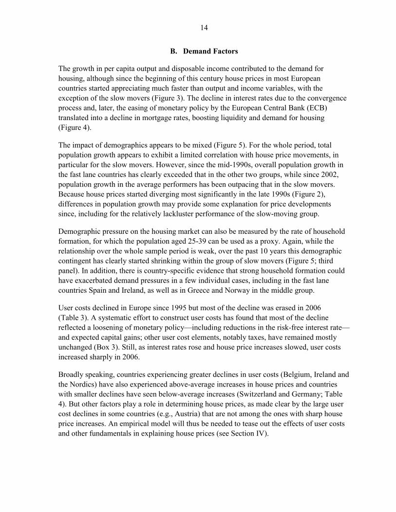
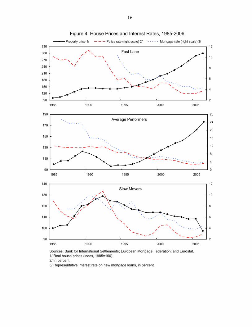
The growth in per capita output and disposable income contributed to the demand for housing, although since the beginning of this century house prices in most European countries started appreciating much faster than output and income variables, with the exception of the slow movers (Figure 3). The decline in interest rates due to the convergence process and, later, the easing of monetary policy by the European Central Bank (ECB) translated into a decline in mortgage rates, boosting liquidity and demand for housing (Figure 4).
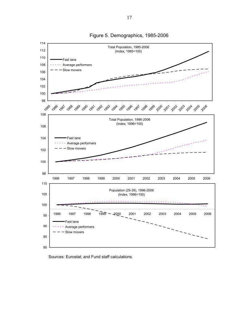
The impact of demographics appears to be mixed (Figure 5). For the whole period, total population growth appears to exhibit a limited correlation with house price movements, in particular for the slow movers. However, since the mid-1990s, overall population growth in the fast lane countries has clearly exceeded that in the other two groups, while since 2002, population growth in the average performers has been outpacing that in the slow movers. Because house prices started diverging most significantly in the late 1990s (Figure 2), differences in population growth may provide some explanation for price developments since, including for the relatively lackluster performance of the slow-moving group.
Demographic pressure on the housing market can also be measured by the rate of household formation, for which the population aged 25-39 can be used as a proxy. Again, while the relationship over the whole sample period is weak, over the past 10 years this demographic contingent has clearly started shrinking within the group of slow movers (Figure 5; third panel). In addition, there is country-specific evidence that strong household formation could have exacerbated demand pressures in a few individual cases, including in the fast lane countries Spain and Ireland, as well as in Greece and Norway in the middle group.
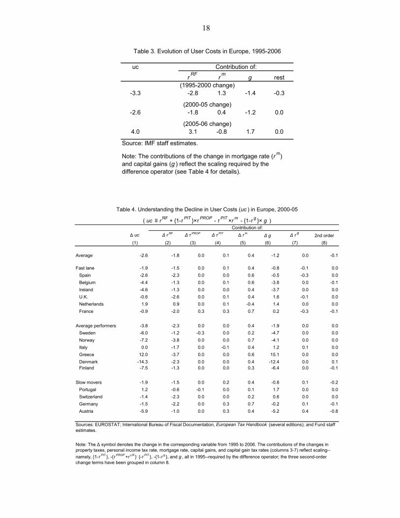
User costs declined in Europe since 1995 but most of the decline was erased in 2006 (Table 3). A systematic effort to construct user costs has found that most of the decline reflected a loosening of monetary policy—including reductions in the risk-free interest rate—and expected capital gains; other user cost elements, notably taxes, have remained mostly unchanged (Box 3). Still, as interest rates rose and house price increases slowed, user costs increased sharply in 2006.
Broadly speaking, countries experiencing greater declines in user costs (Belgium, Ireland and the Nordics) have also experienced above-average increases in house prices and countries with smaller declines have seen below-average increases (Switzerland and Germany; Table 4). But other factors play a role in determining house prices, as made clear by the large user cost declines in some countries (e.g., Austria) that are not among the ones with sharp house price increases. An empirical model will thus be needed to tease out the effects of user costs and other fundamentals in explaining house prices (see Section IV).
15
Figure 3. House Prices and Income, 1985-2006 1/(Index, 1985=100)
Sources: Barclays; Bank for International Settlements; European Mortgage Federation; IMF, World Economic Outlook ; OECD; and IMF staff calculations.1/ All variables are presented as Index 1985=100, corrected for breaks in series.2/ Real house prices.3/ Real per capita GDP (national currency).4/ Real gross disposable income per capita (national currency).
Fast Lane
90
120
150
180
210
240
270
300
330
1985 1990 1995 2000 200590
120
150
180
210
240
270
300
330Property prices 2/ GDP 3/ RDI 4/
Average Performers
90
110
130
150
170
190
1985 1990 1995 2000 200590
110
130
150
170
190
Slow Movers
80
100
120
140
160
180
200
1985 1990 1995 2000 200580
100
120
140
160
180
200
16
Figure 4. House Prices and Interest Rates, 1985-2006
Sources: Bank for International Settlements; European Mortgage Federation; and Eurostat. 1/ Real house prices (index, 1985=100).2/ In percent.3/ Representative interest rate on new mortgage loans, in percent.
Fast Lane
90
120
150
180
210
240
270
300
330
1985 1990 1995 2000 20052
4
6
8
10
12Property price 1/ Policy rate (right scale) 2/ Mortgage rate (right scale) 3/
Average Performers
90
110
130
150
170
190
1985 1990 1995 2000 20050
4
8
12
16
20
24
28
Slow Movers
90
100
110
120
130
140
1985 1990 1995 2000 20052
4
6
8
10
12
17
Figure 5. Demographics, 1985-2006
Sources: Eurostat; and Fund staff calculations.
98
100
102
104
106
108
110
112
114
1985
1986
1987
1988
1989
1990
1991
1992
1993
1994
1995
1996
1997
1998
1999
2000
2001
2002
2003
2004
2005
2006
Fast laneAverage performersSlow movers
Total Population, 1985-2006(Index, 1985=100)
98
100
102
104
106
108
1996 1997 1998 1999 2000 2001 2002 2003 2004 2005 2006
Fast laneAverage performersSlow movers
Total Population, 1996-2006(Index, 1996=100)
80
85
90
95
100
105
110
1996 1997 1998 1999 2000 2001 2002 2003 2004 2005 2006
Fast laneAverage performersSlow movers
Population (25-39), 1996-2006(Index, 1996=100)
18
uc
r RF r m g rest
-3.3 -2.8 1.3 -1.4 -0.3
-2.6 -1.8 0.4 -1.2 0.0
4.0 3.1 -0.8 1.7 0.0
Table 3. Evolution of User Costs in Europe, 1995-2006
Contribution of:
(1995-2000 change)
Note: The contributions of the change in mortgage rate (r m) and capital gains (g ) reflect the scaling required by the difference operator (see Table 4 for details).
(2000-05 change)
(2005-06 change)
Source: IMF staff estimates.
Δ uc Δ r RF Δ τ PROP Δ τ PIT Δ r m Δ g Δ τ g2nd order
(1) (2) (3) (4) (5) (6) (7) (8)
Average -2.6 -1.8 0.0 0.1 0.4 -1.2 0.0 -0.1
Fast lane -1.9 -1.5 0.0 0.1 0.4 -0.8 -0.1 0.0Spain -2.6 -2.3 0.0 0.0 0.6 -0.5 -0.3 0.0Belgium -4.4 -1.3 0.0 0.1 0.6 -3.8 0.0 -0.1Ireland -4.6 -1.3 0.0 0.0 0.4 -3.7 0.0 0.0U.K. -0.6 -2.6 0.0 0.1 0.4 1.6 -0.1 0.0Netherlands 1.9 0.9 0.0 0.1 -0.4 1.4 0.0 0.0France -0.9 -2.0 0.3 0.3 0.7 0.2 -0.3 -0.1
Average performers -3.8 -2.3 0.0 0.0 0.4 -1.9 0.0 0.0Sweden -6.0 -1.2 -0.3 0.0 0.2 -4.7 0.0 0.0Norway -7.2 -3.8 0.0 0.0 0.7 -4.1 0.0 0.0Italy 0.0 -1.7 0.0 -0.1 0.4 1.2 0.1 0.0Greece 12.0 -3.7 0.0 0.0 0.6 15.1 0.0 0.0Denmark -14.3 -2.3 0.0 0.0 0.4 -12.4 0.0 0.1Finland -7.5 -1.3 0.0 0.0 0.3 -6.4 0.0 -0.1
Slow movers -1.9 -1.5 0.0 0.2 0.4 -0.8 0.1 -0.2Portugal 1.2 -0.6 -0.1 0.0 0.1 1.7 0.0 0.0Switzerland -1.4 -2.3 0.0 0.0 0.2 0.6 0.0 0.0Germany -1.5 -2.2 0.0 0.3 0.7 -0.2 0.1 -0.1Austria -5.9 -1.0 0.0 0.3 0.4 -5.2 0.4 -0.8
Table 4. Understanding the Decline in User Costs (uc ) in Europe, 2000-05
Sources: EUROSTAT; International Bureau of Fiscal Documentation, European Tax Handbook (several editions); and Fund staff estimates.
( uc ≡ r RF + {1-τ PIT }×τ PROP - τ PIT ×r m - {1-τ g }× g )Contribution of:
Note: The Δ symbol denotes the change in the corresponding variable from 1995 to 2006. The contributions of the changes in property taxes, personal income tax rate, mortgage rate, capital gains, and capital gain tax rates (columns 3-7) reflect scaling--namely, {1-τ PIT }, -{τ PROP +r LR }, {-τ PIT }, -{1-τ g }, and g , all in 1995--required by the difference operator; the three second-order change terms have been grouped in column 8.
19
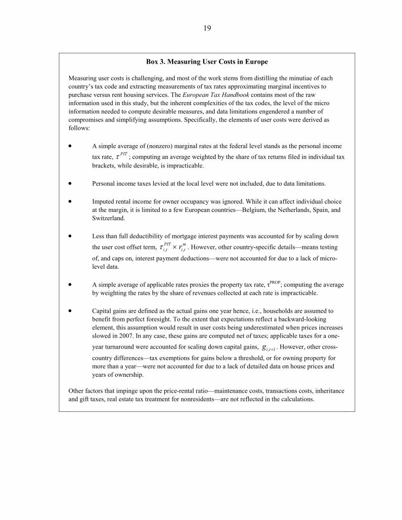
Box 3. Measuring User Costs in Europe
Measuring user costs is challenging, and most of the work stems from distilling the minutiae of each country’s tax code and extracting measurements of tax rates approximating marginal incentives to purchase versus rent housing services. The European Tax Handbook contains most of the raw information used in this study, but the inherent complexities of the tax codes, the level of the micro information needed to compute desirable measures, and data limitations engendered a number of compromises and simplifying assumptions. Specifically, the elements of user costs were derived as follows:
• A simple average of (nonzero) marginal rates at the federal level stands as the personal income
tax rate, PITτ ; computing an average weighted by the share of tax returns filed in individual tax brackets, while desirable, is impracticable.
• Personal income taxes levied at the local level were not included, due to data limitations.
• Imputed rental income for owner occupancy was ignored. While it can affect individual choice at the margin, it is limited to a few European countries—Belgium, the Netherlands, Spain, and Switzerland.
• Less than full deductibility of mortgage interest payments was accounted for by scaling down
the user cost offset term, , ,PIT mi t i trτ × . However, other country-specific details—means testing
of, and caps on, interest payment deductions—were not accounted for due to a lack of micro- level data.
• A simple average of applicable rates proxies the property tax rate, τPROP; computing the average by weighting the rates by the share of revenues collected at each rate is impracticable.
• Capital gains are defined as the actual gains one year hence, i.e., households are assumed to benefit from perfect foresight. To the extent that expectations reflect a backward-looking element, this assumption would result in user costs being underestimated when prices increases slowed in 2007. In any case, these gains are computed net of taxes; applicable taxes for a one-
year turnaround were accounted for scaling down capital gains, , 1i tg + . However, other cross-
country differences—tax exemptions for gains below a threshold, or for owning property for more than a year—were not accounted for due to a lack of detailed data on house prices and years of ownership.
Other factors that impinge upon the price-rental ratio—maintenance costs, transactions costs, inheritance and gift taxes, real estate tax treatment for nonresidents—are not reflected in the calculations.
20
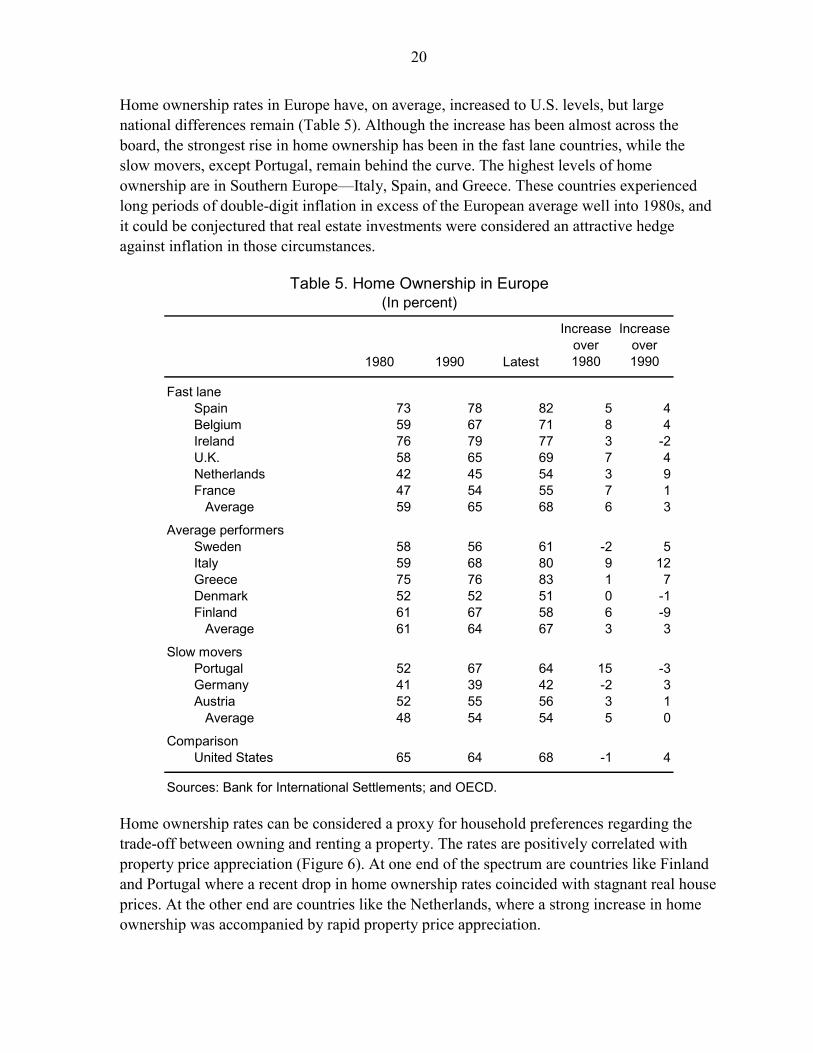
Home ownership rates in Europe have, on average, increased to U.S. levels, but large national differences remain (Table 5). Although the increase has been almost across the board, the strongest rise in home ownership has been in the fast lane countries, while the slow movers, except Portugal, remain behind the curve. The highest levels of home ownership are in Southern Europe—Italy, Spain, and Greece. These countries experienced long periods of double-digit inflation in excess of the European average well into 1980s, and it could be conjectured that real estate investments were considered an attractive hedge against inflation in those circumstances.
1980 1990 Latest
Increase over 1980
Increase over 1990
Fast laneSpain 73 78 82 5 4Belgium 59 67 71 8 4Ireland 76 79 77 3 -2U.K. 58 65 69 7 4Netherlands 42 45 54 3 9France 47 54 55 7 1
Average 59 65 68 6 3
Average performersSweden 58 56 61 -2 5Italy 59 68 80 9 12Greece 75 76 83 1 7Denmark 52 52 51 0 -1Finland 61 67 58 6 -9
Average 61 64 67 3 3
Slow moversPortugal 52 67 64 15 -3Germany 41 39 42 -2 3Austria 52 55 56 3 1
Average 48 54 54 5 0
ComparisonUnited States 65 64 68 -1 4
Sources: Bank for International Settlements; and OECD.
Table 5. Home Ownership in Europe(In percent)
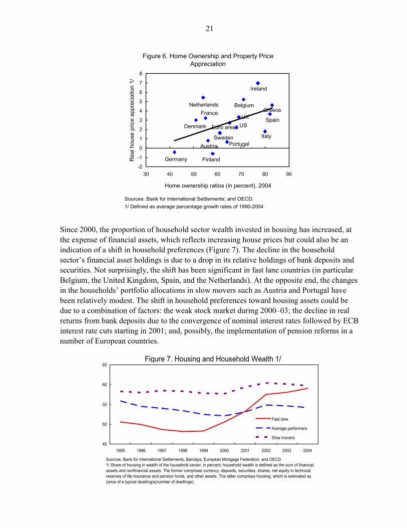
Home ownership rates can be considered a proxy for household preferences regarding the trade-off between owning and renting a property. The rates are positively correlated with property price appreciation (Figure 6). At one end of the spectrum are countries like Finland and Portugal where a recent drop in home ownership rates coincided with stagnant real house prices. At the other end are countries like the Netherlands, where a strong increase in home ownership was accompanied by rapid property price appreciation.
21
Figure 6. Home Ownership and Property Price Appreciation
Sources: Bank for International Settlements; and OECD.1/ Defined as average percentage growth rates of 1990-2004.
Austria
Belgium
Denmark
Finland
France
Germany
Greece
Ireland
Italy
Netherlands
Portugal
Spain
Sweden
UKUSEuro area
-2
-1
0
1
2
3
4
5
6
7
8
30 40 50 60 70 80 90
Home ownership ratios (in percent), 2004
Rea
l hou
se p
rice
appr
ecia
tion
1/
Since 2000, the proportion of household sector wealth invested in housing has increased, at the expense of financial assets, which reflects increasing house prices but could also be an indication of a shift in household preferences (Figure 7). The decline in the household sector’s financial asset holdings is due to a drop in its relative holdings of bank deposits and securities. Not surprisingly, the shift has been significant in fast lane countries (in particular Belgium, the United Kingdom, Spain, and the Netherlands). At the opposite end, the changes in the households’ portfolio allocations in slow movers such as Austria and Portugal have been relatively modest. The shift in household preferences toward housing assets could be due to a combination of factors: the weak stock market during 2000–03; the decline in real returns from bank deposits due to the convergence of nominal interest rates followed by ECB interest rate cuts starting in 2001; and, possibly, the implementation of pension reforms in a number of European countries.
Sources: Bank for International Settlements; Barclays; European Mortgage Federation; and OECD.1/ Share of housing in wealth of the household sector, in percent; household wealth is defined as the sum of financial assets and nonfinancial assets. The former comprises currency, deposits, securities, shares, net equity in technical reserves of life insurance and pension funds, and other assets. The latter comprises housing, which is estimated as (price of a typical dwelling)x(number of dwellings).
45
50
55
60
65
1995 1996 1997 1998 1999 2000 2001 2002 2003 2004
Fast lane
Average performers
Slow movers
Figure 7. Housing and Household Wealth 1/

22
C. Supply Side and Rental Market
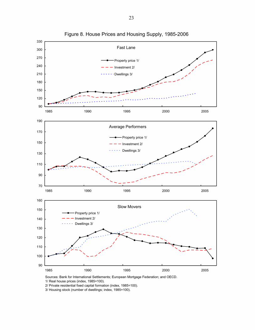
Property price developments in the fast lane and average performers’ groups can also be linked to a muted supply response to the increase in demand for housing (Table 6, Figure 8). It is difficult, however, to measure the degree of supply rigidities across countries and quantify them in a systematic way. Nevertheless, there is anecdotal evidence that structural constraints do exist, including factors such as building regulations, long planning and construction phases, the inertia of existing local land planning schemes, cumbersome zoning regulations and land use restrictions, and slow authorization processes for permits. For instance, while the total stock of housing and number of building permits have picked up, growth has been fairly tepid relative to the house price appreciation in a number of countries (for instance, in the Netherlands and the United Kingdom). These trends are also reflected in the subdued growth of residential investment.
1980s 1990s 2000-04
Fast laneSpain 1.4 1.2 3.4Belgium 0.0 4.5 1.3Ireland 2.0 1.8 6.5U.K. 1.0 0.7 0.7Netherlands 1.9 1.3 0.8France 1.2 1.0 1.0
Average 1.3 1.8 2.3Average performers
Sweden ... 0.6 0.4Italy 1.5 1.0 0.2Greece ... 1.4 2.1Denmark 1.4 0.6 0.6Finland 2.1 1.4 1.2
Average 1.7 1.0 0.9Slow movers
Portugal 2.8 2.2 0.4Germany 0.1 3.9 0.7Austria ... 1.8 5.6
Average 1.4 2.6 2.2
Source: European Mortgage Federation.
Table 6. Housing Stocks (Growth in number of dwellings, in percent)
23
Figure 8. House Prices and Housing Supply, 1985-2006
Sources: Bank for International Settlements; European Mortgage Federation; and OECD. 1/ Real house prices (index, 1985=100).2/ Private residential fixed capital formation (index, 1985=100).3/ Housing stock (number of dwellings; index, 1985=100).
Fast Lane
90
120
150
180
210
240
270
300
330
1985 1990 1995 2000 2005
Property price 1/
Investment 2/
Dwellings 3/
Average Performers
70
90
110
130
150
170
190
1985 1990 1995 2000 2005
Property price 1/
Investment 2/
Dwellings 3/
Slow Movers
90
100
110
120
130
140
150
160
1985 1990 1995 2000 2005
Property price 1/Investment 2/Dwellings 3/

24
Similarly, stagnant property prices in the slow movers could be explained by the supply overhang from strong building activity in the 1990s. Germany is a case in point—until early 2006, the government provided relatively generous subsidies for owner-occupied houses in order to improve housing supply and standards in the New Laender. This large subsidy, provided in response to the inflow of population at the end of the 1980s and early 1990s with the intention of preventing a prolonged increase in house prices, resulted in high levels of residential investment in Germany in the 1990s.
Institutional arrangements in the rental market also have a bearing on house prices. Controls on rents either due to rental contract rigidities or because of government intervention in social housing can depress demand for private dwellings. Alternatively, in a relatively free rental market, housing supply constraints could imply that demand pressures spill into the rental market. In this event, the composition of the total stock of dwellings could be expected to shift toward that segment of the market where prices are increasing more rapidly.
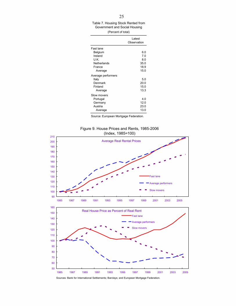
While rental markets in Europe are being liberalized, the pace of liberalization in many countries is slow and, overall, these markets remain highly regulated. A number of countries have introduced greater flexibility in rent increases and the duration and terms of contracts. Ireland led the pack by removing almost all restrictions on rent contracts by the late 1980s. Germany, on the other side, has introduced few reforms in the rental market, although it started allowing greater flexibility in rent increases in 2001.14 Apart from regulation, the role of the government and/or the social housing sector on the supply side of the rental market remains significant in many European countries (Table 7).
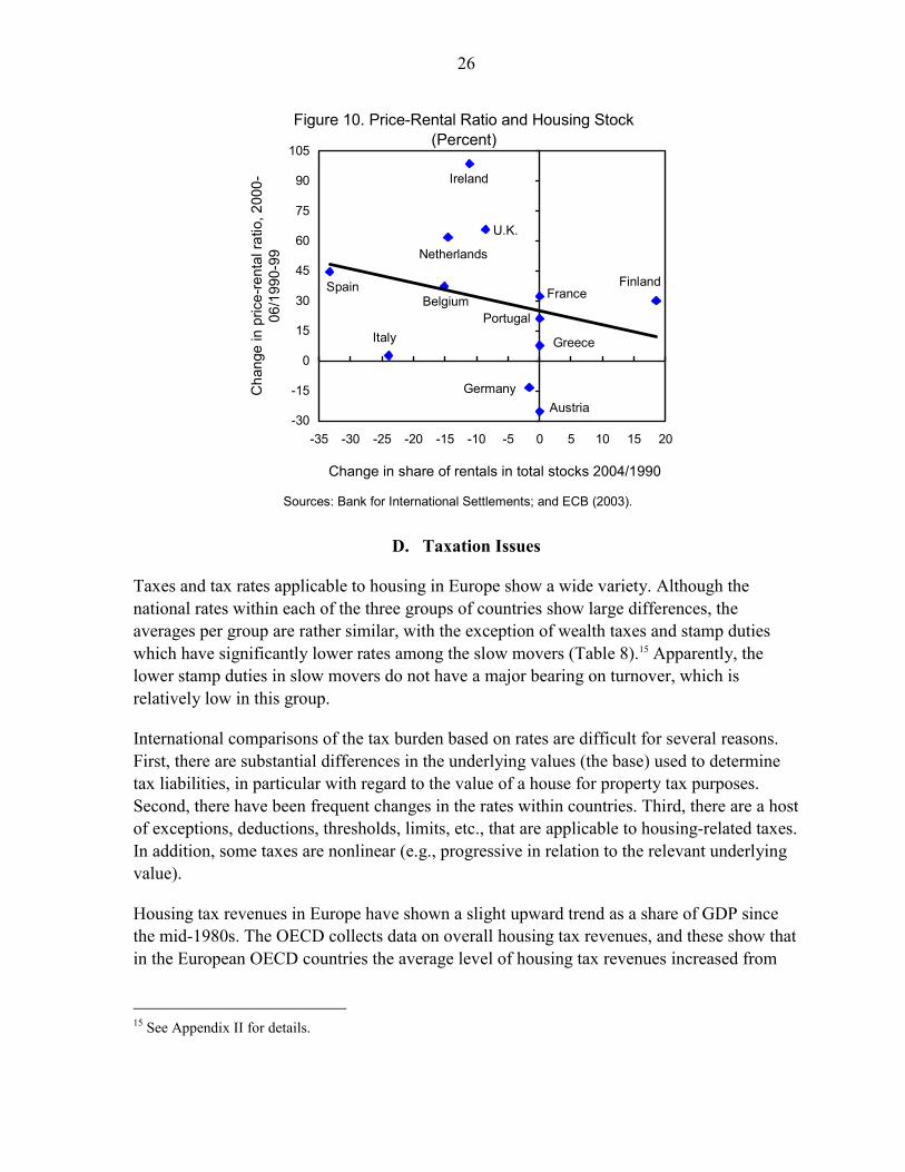
Stocks adjust to relative price changes. Real rents have increased significantly for all three groups, although clearly the least for the slow movers (Figure 9). This suggests that the relative unresponsiveness of housing supply to price increases in the two top groups could have led to a spillover of demand into the rental market. However, the ratio of property prices to rents has increased in the fast lane countries, and the composition of housing stocks has shifted away from rentals in this group (Figure 10). The lower increase in real rents in the slow movers group could be an indication of a relative bias of incentives toward renting rather than purchasing property, due to rigidities in the rental market, the glut on some of the property markets, and the significant role of the government as a landlord. As a result, the share of rented dwellings in housing stocks in most of these countries has remained significant and virtually unchanged. Social preferences are also likely to play a role here.
14 Odenius, Carare, and Crivelli (2008).
25
Figure 9. House Prices and Rents, 1985-2006(Index, 1985=100)
Sources: Bank for International Settlements; Barclays; and European Mortgage Federation.
Average Real Rental Prices
90
100
110
120
130
140
150
160
170
180
190
200
210
1985 1987 1989 1991 1993 1995 1997 1999 2001 2003 2005
Fast lane
Average performers
Slow movers
Real House Price as Percent of Real Rent
50
60
70
80
90
100
110
120
130
140
150
160
1985 1987 1989 1991 1993 1995 1997 1999 2001 2003 2005
Fast lane
Average performers
Slow movers
Latest Observation
Fast laneBelgium 6.0Ireland 7.0U.K. 8.0Netherlands 35.0France 18.9
Average 15.0
Average performersItaly 5.0Denmark 20.0Finland 15.0
Average 13.3
Slow moversPortugal 4.0Germany 12.0Austria 23.0
Average 13.0
Source: European Mortgage Federation.
Table 7. Housing Stock Rented from Government and Social Housing
(Percent of total)
26
D. Taxation Issues
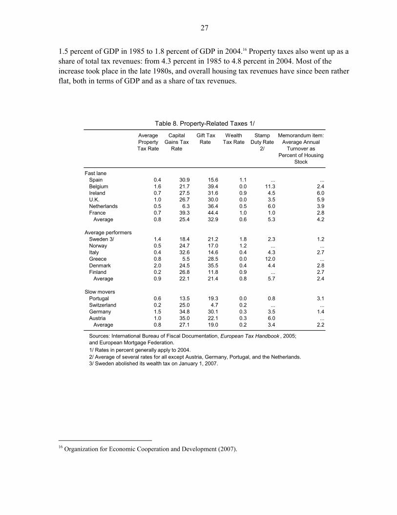
Taxes and tax rates applicable to housing in Europe show a wide variety. Although the national rates within each of the three groups of countries show large differences, the averages per group are rather similar, with the exception of wealth taxes and stamp duties which have significantly lower rates among the slow movers (Table 8).15 Apparently, the lower stamp duties in slow movers do not have a major bearing on turnover, which is relatively low in this group.
International comparisons of the tax burden based on rates are difficult for several reasons. First, there are substantial differences in the underlying values (the base) used to determine tax liabilities, in particular with regard to the value of a house for property tax purposes. Second, there have been frequent changes in the rates within countries. Third, there are a host of exceptions, deductions, thresholds, limits, etc., that are applicable to housing-related taxes. In addition, some taxes are nonlinear (e.g., progressive in relation to the relevant underlying value).
Housing tax revenues in Europe have shown a slight upward trend as a share of GDP since the mid-1980s. The OECD collects data on overall housing tax revenues, and these show that in the European OECD countries the average level of housing tax revenues increased from
15 See Appendix II for details.
Austria
BelgiumFinland
France
Germany
Greece
Ireland
Italy
Netherlands
Portugal
Spain
U.K.
-30
-15
0
15
30
45
60
75
90
105
-35 -30 -25 -20 -15 -10 -5 0 5 10 15 20
Change in share of rentals in total stocks 2004/1990
Cha
nge
in p
rice-
rent
al ra
tio, 2
000-
06/1
990-
99
Sources: Bank for International Settlements; and ECB (2003).
Figure 10. Price-Rental Ratio and Housing Stock(Percent)
27
1.5 percent of GDP in 1985 to 1.8 percent of GDP in 2004.16 Property taxes also went up as a share of total tax revenues: from 4.3 percent in 1985 to 4.8 percent in 2004. Most of the increase took place in the late 1980s, and overall housing tax revenues have since been rather flat, both in terms of GDP and as a share of tax revenues.
Average Property Tax Rate
Capital Gains Tax
Rate
Gift Tax Rate
Wealth Tax Rate
Stamp Duty Rate
2/
Memorandum item: Average Annual
Turnover as Percent of Housing
Stock
Fast laneSpain 0.4 30.9 15.6 1.1 ... ...Belgium 1.6 21.7 39.4 0.0 11.3 2.4Ireland 0.7 27.5 31.6 0.9 4.5 6.0U.K. 1.0 26.7 30.0 0.0 3.5 5.9Netherlands 0.5 6.3 36.4 0.5 6.0 3.9France 0.7 39.3 44.4 1.0 1.0 2.8
Average 0.8 25.4 32.9 0.6 5.3 4.2
Average performersSweden 3/ 1.4 18.4 21.2 1.8 2.3 1.2Norway 0.5 24.7 17.0 1.2 ... ...Italy 0.4 32.6 14.6 0.4 4.3 2.7Greece 0.8 5.5 28.5 0.0 12.0 ...Denmark 2.0 24.5 35.5 0.4 4.4 2.8Finland 0.2 26.8 11.8 0.9 ... 2.7
Average 0.9 22.1 21.4 0.8 5.7 2.4
Slow moversPortugal 0.6 13.5 19.3 0.0 0.8 3.1Switzerland 0.2 25.0 4.7 0.2 ... ...Germany 1.5 34.8 30.1 0.3 3.5 1.4Austria 1.0 35.0 22.1 0.3 6.0 ...
Average 0.8 27.1 19.0 0.2 3.4 2.2
Sources: International Bureau of Fiscal Documentation, European Tax Handbook , 2005; and European Mortgage Federation.1/ Rates in percent generally apply to 2004.2/ Average of several rates for all except Austria, Germany, Portugal, and the Netherlands.3/ Sweden abolished its wealth tax on January 1, 2007.
Table 8. Property-Related Taxes 1/
16 Organization for Economic Cooperation and Development (2007).

28
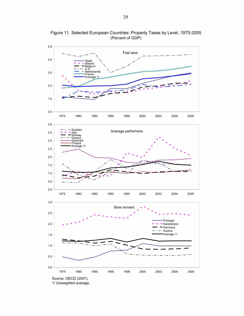
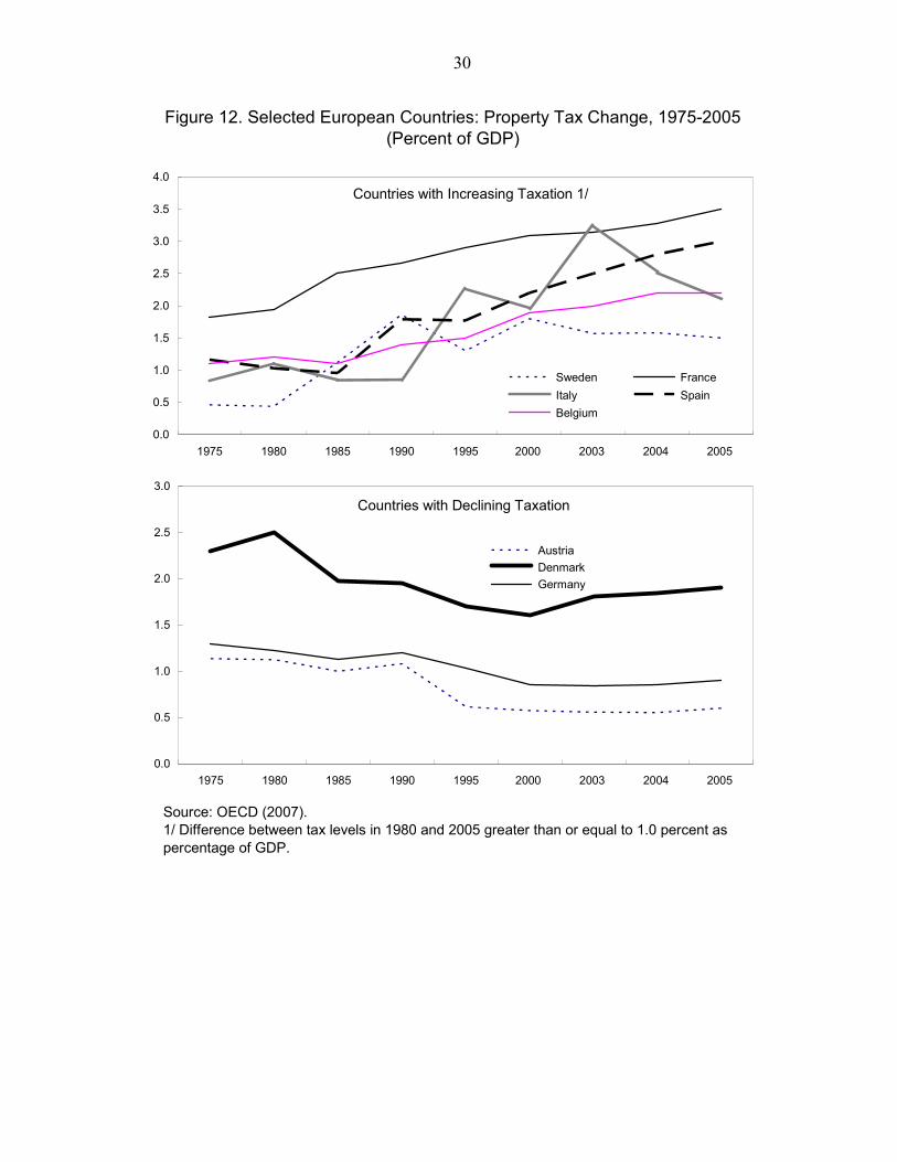
National property tax revenues show a wide variety, both in level and in development (Figures 11 and 12). Nor surprisingly, fast lane countries such as France and Spain show high revenues and the United Kingdom comes out on top, with tax revenues in recent years amounting to 4-5 percent of GDP. These are also among the countries with the fastest increases in tax revenues (Figure 12). At the same time, Germany and Austria had the lowest levels of housing tax revenues, whereas these two countries were also among the few that showed declining revenues. On average, fast lane countries have property tax revenues exceeding 2 percent of GDP, the average performers record revenues of about 1.5 percent of GDP (at least in recent years), and the slow movers show stable average tax revenues in the order of 1¼ percent of GDP.
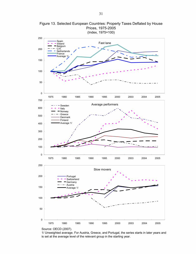
When tax revenues are corrected for developments in house prices, as a proxy for the tax burden on housing, they show an upward movement until 2000 and a decline thereafter. Figure 13, which includes property taxes deflated by house price developments, indicates that this burden had been increasing over the years, but only until about 2000, when for the fast lane countries and the average performers a decline set in, while the average for the slow movers was basically flat.
A few points about individual countries are worth noting. Despite having a rather light and declining overall housing tax burden (Figure 11), Germany has a relatively high property tax rate and is one of the few countries in the sample that does not allow mortgage interest payment deductions. Belgium and Denmark have seen strong increases in property prices in recent years, despite the relatively high tax rates in these countries.17 The decline in property taxes coincided with property price increases in France, Greece and Ireland, although this was counteracted by a reduction in the rate of mortgage interest rate deductibility in the latter two countries.18 A number of housing markets in fast lane countries, such as Spain and the Netherlands, enjoy relatively low property tax rates and, in particular in the case of the Netherlands, a relatively generous regime of mortgage interest deductibility for income taxation.
17 For Denmark, it is relevant to note that the frozen and therefore increasingly below-market valuation of property in determining property taxes contributed to the upward pressures. Recently, house prices in Denmark have come under downward pressures.
18 The rate had been steadily reduced in France until deductibility was partially reinstated in 2007; it was more than halved in Greece in the mid-1990s.
29
Figure 11. Selected European Countries: Property Taxes by Level, 1975-2005(Percent of GDP)
Source: OECD (2007).1/ Unweighted average.
0.0
1.0
2.0
3.0
4.0
5.0
1975 1980 1985 1990 1995 2000 2003 2004 2005
SpainIrelandBelgiumU.K.NetherlandsFranceAverage 1/
Fast lane
0.0
0.5
1.0
1.5
2.0
2.5
3.0
3.5
4.0
1975 1980 1985 1990 1995 2000 2003 2004 2005
SwedenItalyNorwayGreeceDenmarkFinlandAverage 1/
Average performers
0.0
0.5
1.0
1.5
2.0
2.5
3.0
1975 1980 1985 1990 1995 2000 2003 2004 2005
PortugalSwitzerlandGermanyAustriaAverage 1/
Slow movers
30
Figure 12. Selected European Countries: Property Tax Change, 1975-2005(Percent of GDP)
Source: OECD (2007).1/ Difference between tax levels in 1980 and 2005 greater than or equal to 1.0 percent as percentage of GDP.
0.0
0.5
1.0
1.5
2.0
2.5
3.0
3.5
4.0
1975 1980 1985 1990 1995 2000 2003 2004 2005
Sweden France Italy Spain Belgium
Countries with Increasing Taxation 1/
0.0
0.5
1.0
1.5
2.0
2.5
3.0
1975 1980 1985 1990 1995 2000 2003 2004 2005
Austria Denmark Germany
Countries with Declining Taxation
31
Figure 13. Selected European Countries: Property Taxes Deflated by House Prices, 1975-2005 (Index, 1975=100)
Source: OECD (2007).1/ Unweighted average. For Austria, Greece, and Portugal, the series starts in later years and is set at the average level of the relevant group in the starting year.
0
50
100
150
200
250
1975 1980 1985 1990 1995 2000 2003 2004 2005
SpainIrelandBelgiumU.K.NetherlandsFranceAverage 1/
Fast lane
0
100
200
300
400
500
600
700
1975 1980 1985 1990 1995 2000 2003 2004 2005
SwedenItalyNorwayGreeceDenmarkFinlandAverage 1/
Average performers
0
50
100
150
200
250
1975 1980 1985 1990 1995 2000 2003 2004 2005
PortugalSwitzerlandGermanyAustriaAverage 1/
Slow movers

32
E. Financial Sector
The literature points to a number of characteristics of the housing finance sector that are relevant for price developments in housing markets:19
• the structure of the supply side, i.e., the relative role of general banks, specialized (mortgage) banks, credit unions, brokers, and nonbank suppliers of housing finance;
• the flexibility of the products offered with regard to maturity, interest rate flexibility, repayment schemes, and refinancing options;
• the presence and size of subprime mortgage markets;
• transaction costs (brokers’ fees, banks’ and legal fees, points, etc.);
• the existence of a secondary market for mortgages and/or a MBS market;
• the degree of financial liberalization;
• supervisory rules and regulations (LTV and LTI ratios, CARs, etc.); and
• collateral legislation and practices.
It is difficult, however, to construct aggregate indicators that capture the degree of development, efficiency and flexibility of housing finance systems, and reliable information on the indicators listed above is not available on a systematic basis for all countries in the sample.20 This section therefore relies on two types of proxies that are used in other studies. The first one is the share of property-related lending in GDP, which can be considered an indicator of the depth of the mortgage market. The second is a synthetic mortgage market development or “completeness” indicator, which measures the range of products and the flexibility of mortgage markets. Unfortunately, these indicators are only available for specific years and for a subset of countries.
Financial sector lending for property increased in all European countries except Sweden (Figure 14). However, in the slow movers, lending did not increase as rapidly as it did in the fast lane countries.21 By and large, the rate of increase in mortgage lending exceeded the growth in property prices (Figure 15).
19 Committee on the Global Financial System (2006), European Mortgage Federation (2004, 2006b-c), European Commission (2005), and European Central Bank (2003).
20 Indicators for the overall development of the financial sector—see, e.g., Abiad and Mody (2003)—do not generally capture the specific development of the mortgage market.
21 The direction of the causality, however, is not obvious: more conservative financial systems may have kept prices in check through reduced supply of credit, but also the slow pace of house prices may have limited demand for housing finance.
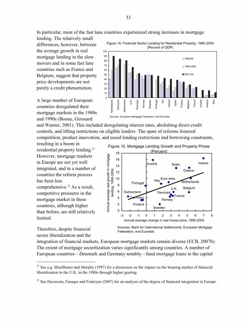
33
In particular, most of the fast lane countries experienced strong increases in mortgage lending. The relatively small differences, however, between the average growth in real mortgage lending in the slow movers and in some fast lane countries such as France and Belgium, suggest that property price developments are not purely a credit phenomenon. A large number of European countries deregulated their mortgage markets in the 1980s and 1990s (Boone, Girouard and Warner, 2001). This included deregulating interest rates, abolishing direct credit controls, and lifting restrictions on eligible lenders. The spate of reforms fostered competition, product innovation, and eased lending restrictions and borrowing constraints, resulting in a boom in residential property lending.22 However, mortgage markets in Europe are not yet well integrated, and in a number of countries the reform process has been less comprehensive.23 As a result, competitive pressures in the mortgage market in these countries, although higher than before, are still relatively limited.
Therefore, despite financial sector liberalization and the integration of financial markets, European mortgage markets remain diverse (ECB, 2007b). The extent of mortgage securitization varies significantly among countries. A number of European countries—Denmark and Germany notably—fund mortgage loans in the capital 22 See e.g. Muellbauer and Murphy (1997) for a discussion on the impact on the housing market of financial liberalization in the U.K. in the 1980s through higher gearing.
23 See Decressin, Faruqee and Fonteyne (2007) for an analysis of the degree of financial integration in Europe.
Figure 14. Financial Sector Lending for Residential Property, 1990-2004(Percent of GDP)
Sources: European Mortgage Federation; and Eurostat.
0
10
20
30
40
50
60
70
80
90
100
Net
herla
nds
Den
mar
k
Switz
erla
nd
U.K
.
Ger
man
y
Nor
way
Swed
en
Por
tuga
l
EU
Irela
nd
Spa
in
Finl
and
Bel
gium
Fran
ce
Aus
tria
Gre
ece
Italy
1990-94
1995-2000
2001-04
Austria
BelgiumDenmark
Finland
FranceGermany
Greece
Ireland
Italy Netherlands
Norway
Portugal
Spain
Sweden
SwitzerlandU.K.
Euro area
0
2
4
6
8
10
12
14
16
18
-3 -2 -1 0 1 2 3 4 5 6 7 8Annual average change in real house price, 1990-2004
Ann
ual a
vera
ge re
al g
row
th in
mor
tgag
e le
ndin
g, 1
990-
2004
Figure 15. Mortgage Lending Growth and Property Prices(Percent)
Sources: Bank for International Settlements; European Mortgage Federation; and Eurostat.
34
markets using bonds (e.g., the German Pfandbriefe). These bonds differ from mortgage-backed securities as they remain on the balance sheet of the issuer, thereby limiting the extent of risk transfer by originating banks.
The degree of sophistication of a country’s mortgage market will affect the demand for housing. The greater the range and flexibility of the financial instruments offered, the more affordable housing can become for a given level of income. Ceteris paribus, this will increase demand for housing. The ability of financial institutions to offer more flexibility in housing finance is determined, inter alia, by collateral legislation and the extent to which mortgage loans can be securitized in order to pool and diversify risks from individual borrowers.
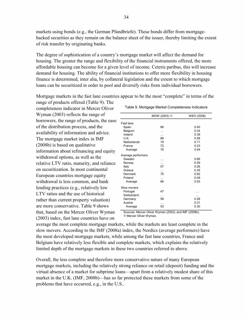
Mortgage markets in the fast lane countries appear to be the most “complete” in terms of the range of products offered (Table 9). The completeness indicator in Mercer Oliver Wyman (2003) reflects the range of borrowers, the range of products, the ease of the distribution process, and the availability of information and advice. The mortgage market index in IMF (2008b) is based on qualitative information about refinancing and equity withdrawal options, as well as the relative LTV ratio, maturity, and reliance on securitization. In most continental European countries mortgage equity withdrawal is less common, and bank lending practices (e.g., relatively low LTV ratios and the use of historical rather than current property valuation) are more conservative. Table 9 shows that, based on the Mercer Oliver Wyman (2003) index, fast lane countries have on average the most complete mortgage markets, while the markets are least complete in the slow movers. According to the IMF (2008a) index, the Nordics (average performers) have the most developed mortgage markets, while among the fast lane countries, France and Belgium have relatively less flexible and complete markets, which explains the relatively limited depth of the mortgage markets in these two countries referred to above.
Overall, the less complete and therefore more conservative nature of many European mortgage markets, including the relatively strong reliance on retail (deposit) funding and the virtual absence of a market for subprime loans—apart from a relatively modest share of this market in the U.K. (IMF, 2008b)—has so far protected these markets from some of the problems that have occurred, e.g., in the U.S..
MOW (2003) 1/ WEO (2008)
Fast laneSpain 66 0.40Belgium … 0.34Ireland … 0.39U.K. 86 0.58Netherlands 79 0.71France 72 0.23
Average 76 0.44
Average performersSweden … 0.66Norway … 0.59Italy 57 0.26Greece … 0.35Denmark 75 0.82Finland … 0.49
Average 66 0.53
Slow moversPortugal 47 …Switzerland … …Germany 58 0.28Austria … 0.31
Average 53 0.30
Sources: Mercer Oliver Wyman (2003); and IMF (2008b).1/ Mercer Oliver Wyman.
Table 9. Mortgage Market Completeness Indicators
35
IV. ASSESSING HOUSE PRICE DEVELOPMENTS: AN EMPIRICAL APPROACH
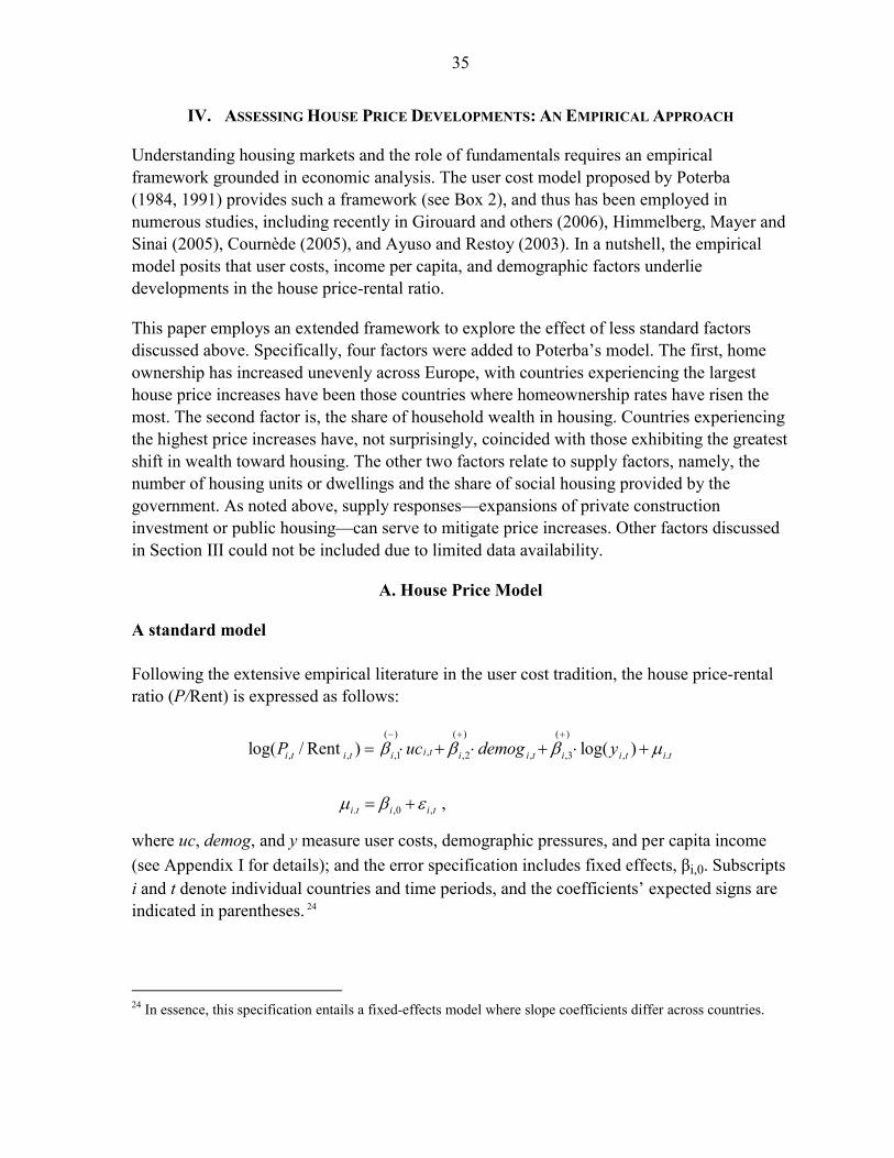
Understanding housing markets and the role of fundamentals requires an empirical framework grounded in economic analysis. The user cost model proposed by Poterba (1984, 1991) provides such a framework (see Box 2), and thus has been employed in numerous studies, including recently in Girouard and others (2006), Himmelberg, Mayer and Sinai (2005), Cournède (2005), and Ayuso and Restoy (2003). In a nutshell, the empirical model posits that user costs, income per capita, and demographic factors underlie developments in the house price-rental ratio.
This paper employs an extended framework to explore the effect of less standard factors discussed above. Specifically, four factors were added to Poterba’s model. The first, home ownership has increased unevenly across Europe, with countries experiencing the largest house price increases have been those countries where homeownership rates have risen the most. The second factor is, the share of household wealth in housing. Countries experiencing the highest price increases have, not surprisingly, coincided with those exhibiting the greatest shift in wealth toward housing. The other two factors relate to supply factors, namely, the number of housing units or dwellings and the share of social housing provided by the government. As noted above, supply responses—expansions of private construction investment or public housing—can serve to mitigate price increases. Other factors discussed in Section III could not be included due to limited data availability.
A. House Price Model
A standard model
Following the extensive empirical literature in the user cost tradition, the house price-rental ratio (P/Rent) is expressed as follows:
( ) ( ) ( )
,, , ,1 ,2 ,3 ., ,
. ,0 ,
log( / Rent ) log( )
,
i ti t i t i i i i ti t i t
i t i i t
P uc demog yβ β β μ
μ β ε
− + +
= ⋅ + ⋅ + ⋅ +
= +
where uc, demog, and y measure user costs, demographic pressures, and per capita income (see Appendix I for details); and the error specification includes fixed effects, βi,0. Subscripts i and t denote individual countries and time periods, and the coefficients’ expected signs are indicated in parentheses. 24
24 In essence, this specification entails a fixed-effects model where slope coefficients differ across countries.
36
A variation of this model is also considered. Rigidities in European rental markets (Section III.C) limit the informational content of rental rates and motivate a second version of the model with house prices, P, as the dependent variable, namely,
( ) ( ) ( )
,, ,1 ,2 ,3 ., ,
. ,0 ,
log( ) log( )
.
i ti t i i i i ti t i t
i t i i t
P uc demog yβ β β μ
μ β ε
− + +
= ⋅ + ⋅ + ⋅ +
= +
The panel estimation techniques employed to estimate these models exploit cross-country differences. In particular, the estimation follows Pedroni (2001) who proposes a mean group estimator (MGE) of dynamic ordinary least squares (DOLS) (Stock and Watson, 1993). The MGE has a distinct advantage when slope coefficients are heterogeneous across countries (as is likely to be the case here): it provides consistent estimates of the sample mean of the heterogeneous cointegrating vectors; pooled-within-dimension (fixed-effects) estimators do not (Pesaran and Smith, 1995). In addition, hypothesis testing for the MGE can proceed without imposing the unappealing restriction that countries share a common coefficient value under the alternative hypothesis. DOLS estimation provides a single-equation method—correcting for the small sample effects of serial autocorrelation and endogeneity—to estimate long-run (cointegrating) models that are asymptotically equivalent to full information maximum likelihood estimators (Johansen, 1988 and 1991).25
The specification of the standard model also intrinsically captures a range of country-specific features contributing to house price developments. Specifically, a built-in layer of cross-country idiosyncrasy stems from the varying effect of interest rates on the price-rental ratio, despite the high degree of comovement in European interest rates noted above. Consider an increase in the risk-free interest rate, rRF, that, through its impact on the user cost, uc, reduces the long-run price-rental ratio. Although the increase in rRF is common across countries, the decline in the price-rental ratio in each country will reflect differences in the tax code and the financial system (it will also reflect cross-country differences in ,1iβ ). Specifically, the price-rental ratio response—holding constant other fundamentals—is captured by the following formula:26
25 The correction augments the long-run equation with auxiliary regressors, namely the leads and lags of the first differences of all right-hand-side variables; the number of leads and lags included is determined empirically by testing down for the highest significant lead and lag.
26 The partial derivative was obtained using the expression for user costs in Box 2, which was substituted into the price-rental ratio equation in the text. As discussed below, the full effect (total differential) of an increase in the interest rate would also include the effect of interest rates on output.
37
( )
( ), , ,
,1
( )
,1 ,
log( / Rent )
1 1 0 .
i t i t i tiRF RF
mPIT i
i i t RF
P ucr r
rr
β
β τ
−
−
∂ ∂= ⋅
∂ ∂⎡ ⎤∂
= ⋅ + − ⋅ <⎢ ⎥∂⎣ ⎦
The decline in the price-rental ratio thus stems from the higher opportunity cost of “investing” in a house (the first term in square brackets), which is common across countries, and the additional (net) cost of servicing mortgage debt (the second term). The latter reflects the mitigating effects of personal income tax deductions, (1 )PIT
iτ− and the degree of
transmission of policy rates to mortgage interest rates, m RFir r∂ ∂ ; both are country specific.27
These models can help us to understand the role that fundamentals play in housing developments. Consider the fitted value of the price-rental ratio,
,, , 1 2 3 ,0, ,ˆ ˆ ˆ ˆlog( / Rent ) log( )FITTED
i ti t i t iti t i tP uc demog yβ β β β= ⋅ + ⋅ + ⋅ + ,
where the symbol “^” denotes the panel estimates. Tracing out the fitted value and its components—namely, 1 ,
ˆi tucβ ⋅ , 2 ,
ˆi tdemogβ ⋅ , and 3 ,
ˆ log( )i tyβ ⋅ —provides an assessment of the importance of the individual fundamentals underlying equilibrium housing market developments. These components are not necessarily independent, however, and thus the breakdown provides no more than an accounting framework to examine these developments. In other words, the breakdown does not properly apportion the indirect effects of either interest rates or output, that is, the effect of interest rates on output and the policy response of interest rates to output.
An extended model
Exploring the effects of nonstandard factors requires adjusting the empirical methodology. This is because these data provide a snapshot of these factors. In the extreme (a single time-invariant observation), their effects cannot be disentangled (identified): the effect is subsumed in the country’s fixed effect. Although formally the effect could be recovered with two observations, these estimates would be suspect as they would rely on a limited amount of information to achieve identification. To overcome this issue, this study relies on Hausman 27 In general, this formula assumes that tax rates are not a function of rRF and that expected capital gains are
invariant to changes in the risk-free rate, that is, / 0RFg r∂ ∂ = . Relaxing the latter restriction adds a third term
to the brackets, namely, ( ),1 0g ii t RF
gr
τ ∂− − ⋅ >
∂, and thus strengthens the inverse relation between the house
price-rental ratio and rRF.
38
and Taylor ‘s (1981) estimation and quantifies the time-invariant effects using the following extended model:
( ) ( ) ( )
,, , 1 2 3 ., ,
. ,0 ,
log( / Rent ) log( )
,
i ti t i t i ti t i t
i t i i t
P uc demog y Zβ β β γ μ
μ β ε
− + +
= ⋅ + ⋅ + ⋅ + +
= +
where Z represents the four nonstandard (time-invariant) factors noted above. The estimation procedure entails feasible generalized least squares (GLS) implemented in three steps. First, within estimates of the β’s are used to obtain initial estimates of μi,t. Second, the latter terms are averaged over time and used to obtain two stage least squares (2SLS) estimates of γ. And third, the feasible GLS estimates for the full model—based on the estimates of error components of the within and time averages—are obtained using weighted 2SLS. Note, however, that the identification of the effect of Z comes at a price: slope homogeneity.28 Thus, to ensure that these estimates are valid, the extended models are subject to “poolability” tests (Pesaran and Yamagata, 2008).
Assessing valuation
Before turning to the empirical results, it is important to stress that judging the extent to which prices are over-or undervalued will reflect one’s beliefs on where fundamentals are heading and how far these will go in the long run. Regardless of the model used to judge house prices, the analyst, either explicitly or implicitly, must take a stand on the (long-run) values of fundamentals. This is unavoidable because of the need to establish a (long-run) benchmark for house prices that, by construction, is conditional on fundamentals. Consider the standard model discussed above. A natural measure of (over) valuation (in percent) would be the difference of the (log) price rental ratio today and the model’s (long-run) forecast:
( ) ( ) ( )( ) ( )
, , , , ,
( ) ( ) ( ),
,1 , i ,2 , i ,3 ,i
/ Rent , , log / Rent log / Rent
ˆ ˆ ˆ ˆlog ,
i t i t i t i i i i t i t i i
i ti i t i i t i i t
OVER P uc demog y P P
yuc uc demog demog
yβ β β ε− + +
= −
⎛ ⎞= ⋅ − + ⋅ − + ⋅ +⎜ ⎟⎜ ⎟
⎝ ⎠
where the (conditional) forecast of the price rental ratio ( / Renti iP ) has been evaluated using
the long-run, or expected, values of the fundamentals, namely, iuc , idemog , and iy . For the
28 Formally, the identification requires that the number of exogenous time-varying instruments exceeds the number of time-invariant regressors.

39
discussion below, it is important to stress that OVER comprises two parts, the model’s inability to track the data, ,i tε and the contribution of fundamentals. The latter component reflects the fundamentals’ deviation from their long-run values, which are scaled by the corresponding coefficient estimates.29 A valuation assessment differs from an assessment of whether house prices exhibit a bubble, which “is a fuzzy word filled with import but lacking a solid operational definition,” (Garber, 2001; see Box 4).
Box 4. Do Housing Prices Reflect A Bubble?
In posing this question, a typical investor would like to know whether house prices will collapse in order to avoid capital losses. A more sophisticated investor would like to know whether the probability of a collapse in house prices outweighs expected capital gains. A rational (and risk-neutral) investor knows, however, that expected capital gains are zero, even if house prices are not only driven by fundamentals because, in well-functioning markets, arbitrage opportunities are squeezed out (no arbitrage condition).
Accordingly, the literature has developed two types of bubbles:
• Irrational bubbles can arise if the market, in addition to rational investors, includes so-called noise traders—agents trading for reasons not modeled, such as herding behavior. In these cases, a natural measure of a bubble would be the difference between the market price and the price that would have arisen had all investors been rational. A persistent difference between these prices can result from (risk-averse) rational investors eschewing arbitrage opportunities from minor price misalignments or from the prevalence of noise traders in the market.
• Rational bubbles can arise, just as in other asset prices, because house prices today reflect tomorrow’s capital gains and rental income. Under forward-looking expectations, this implies that house prices can be expressed as the sum of a fundamental price (the discounted sum of future rental income) and a bubble (the present value of the house price in the distant future), namely, P F B= + . To rule out
excess arbitrage opportunities, these bubbles evolve as follows: 11(1 ) [ ]tB r E B−+= + × , where r is the
real interest rate. For this expression to hold, explosive bubbles must increase at rate r; periodically collapsing bubbles must increase at higher rates. Bubbles can also vary randomly (stochastic bubbles) and be correlated with fundamentals (intrinsic bubbles).
A number of tests have been developed to detect price bubbles, but several weaknesses remain unsolved. Variance-bound tests check for excess volatility in observed prices compared with that expected in the absence of a bubble. These tests, however, do not distinguish between improper model specification and a bubble. West’s two-step test exploits the no-arbitrage condition to separate the model specification test from the bubble test. This test relies on estimation bias arising from the correlation of bubbles and fundamentals, that is, the test has power in detecting intrinsic bubbles. The time-series properties of stochastic bubbles—nonstationary even after ndifferences—form the basis of unit root and cointegration-based tests. While useful in detecting explosive bubbles, periodically collapsing bubbles are more challenging to detect as these resemble mean-reverting prices.
29 Only when the conditional forecast is evaluated using the fundamentals’ current values—
, , ,, and i t i i t i i t iuc uc cc cc y y= = = —would valuation be measured only by the residual.
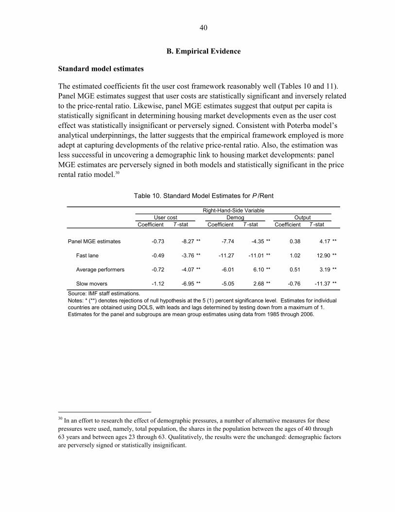
40
B. Empirical Evidence
Standard model estimates
The estimated coefficients fit the user cost framework reasonably well (Tables 10 and 11). Panel MGE estimates suggest that user costs are statistically significant and inversely related to the price-rental ratio. Likewise, panel MGE estimates suggest that output per capita is statistically significant in determining housing market developments even as the user cost effect was statistically insignificant or perversely signed. Consistent with Poterba model’s analytical underpinnings, the latter suggests that the empirical framework employed is more adept at capturing developments of the relative price-rental ratio. Also, the estimation was less successful in uncovering a demographic link to housing market developments: panel MGE estimates are perversely signed in both models and statistically significant in the price rental ratio model.30
30 In an effort to research the effect of demographic pressures, a number of alternative measures for these pressures were used, namely, total population, the shares in the population between the ages of 40 through 63 years and between ages 23 through 63. Qualitatively, the results were the unchanged: demographic factors are perversely signed or statistically insignificant.
Coefficient T -stat Coefficient T -stat Coefficient T -stat
Panel MGE estimates -0.73 -8.27 ** -7.74 -4.35 ** 0.38 4.17 **
Fast lane -0.49 -3.76 ** -11.27 -11.01 ** 1.02 12.90 **
Average performers -0.72 -4.07 ** -6.01 6.10 ** 0.51 3.19 **
Slow movers -1.12 -6.95 ** -5.05 2.68 ** -0.76 -11.37 **
Table 10. Standard Model Estimates for P /Rent
Notes: * (**) denotes rejections of null hypothesis at the 5 (1) percent significance level. Estimates for individual countries are obtained using DOLS, with leads and lags determined by testing down from a maximum of 1. Estimates for the panel and subgroups are mean group estimates using data from 1985 through 2006.
User costRight-Hand-Side Variable
Demog Output
Source: IMF staff estimations.
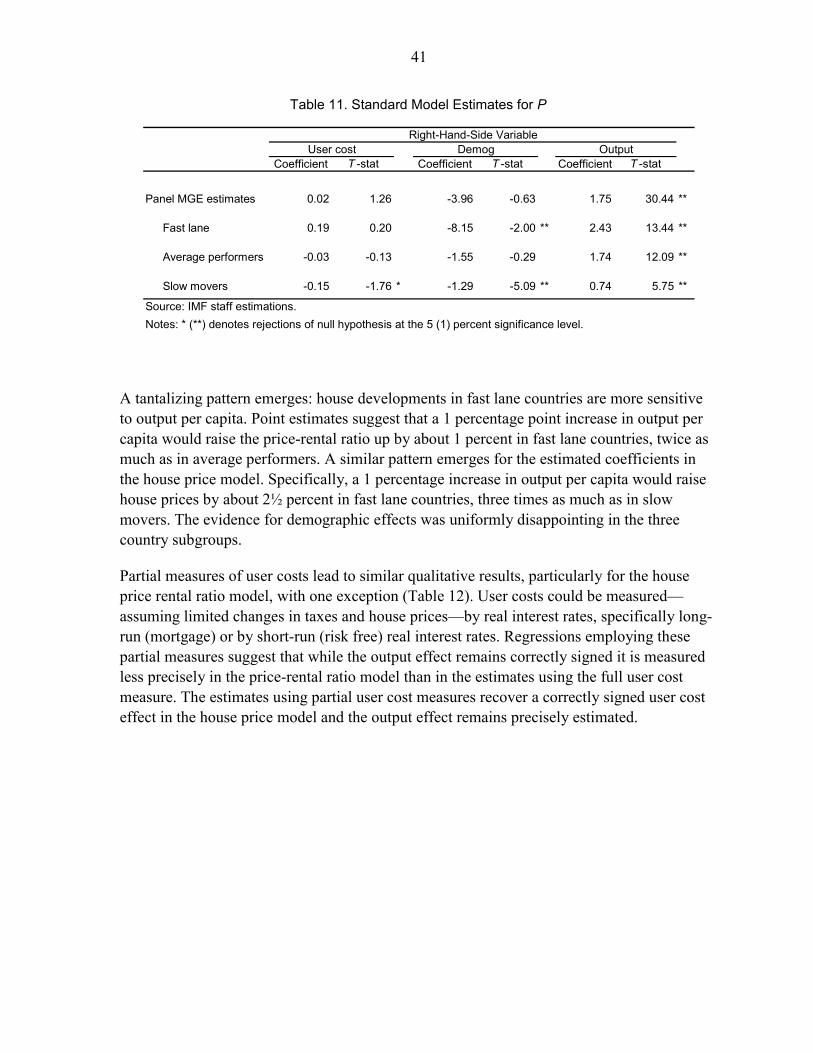
41
A tantalizing pattern emerges: house developments in fast lane countries are more sensitive to output per capita. Point estimates suggest that a 1 percentage point increase in output per capita would raise the price-rental ratio up by about 1 percent in fast lane countries, twice as much as in average performers. A similar pattern emerges for the estimated coefficients in the house price model. Specifically, a 1 percentage increase in output per capita would raise house prices by about 2½ percent in fast lane countries, three times as much as in slow movers. The evidence for demographic effects was uniformly disappointing in the three country subgroups.
Partial measures of user costs lead to similar qualitative results, particularly for the house price rental ratio model, with one exception (Table 12). User costs could be measured—assuming limited changes in taxes and house prices—by real interest rates, specifically long-run (mortgage) or by short-run (risk free) real interest rates. Regressions employing these partial measures suggest that while the output effect remains correctly signed it is measured less precisely in the price-rental ratio model than in the estimates using the full user cost measure. The estimates using partial user cost measures recover a correctly signed user cost effect in the house price model and the output effect remains precisely estimated.
Coefficient T -stat Coefficient T -stat Coefficient T -stat
Panel MGE estimates 0.02 1.26 -3.96 -0.63 1.75 30.44 **
Fast lane 0.19 0.20 -8.15 -2.00 ** 2.43 13.44 **
Average performers -0.03 -0.13 -1.55 -0.29 1.74 12.09 **
Slow movers -0.15 -1.76 * -1.29 -5.09 ** 0.74 5.75 **
Table 11. Standard Model Estimates for P
Notes: * (**) denotes rejections of null hypothesis at the 5 (1) percent significance level.
User costRight-Hand-Side Variable
Demog Output
Source: IMF staff estimations.
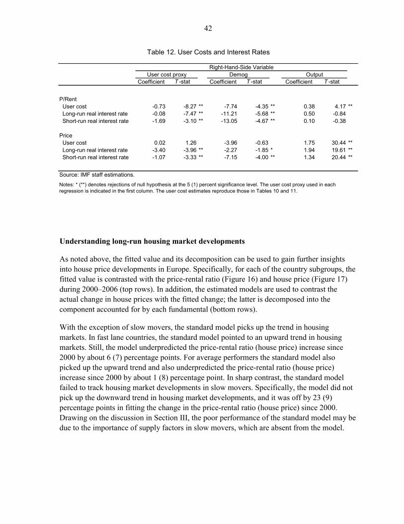
42
Understanding long-run housing market developments
As noted above, the fitted value and its decomposition can be used to gain further insights into house price developments in Europe. Specifically, for each of the country subgroups, the fitted value is contrasted with the price-rental ratio (Figure 16) and house price (Figure 17) during 2000–2006 (top rows). In addition, the estimated models are used to contrast the actual change in house prices with the fitted change; the latter is decomposed into the component accounted for by each fundamental (bottom rows).
With the exception of slow movers, the standard model picks up the trend in housing markets. In fast lane countries, the standard model pointed to an upward trend in housing markets. Still, the model underpredicted the price-rental ratio (house price) increase since 2000 by about 6 (7) percentage points. For average performers the standard model also picked up the upward trend and also underpredicted the price-rental ratio (house price) increase since 2000 by about 1 (8) percentage point. In sharp contrast, the standard model failed to track housing market developments in slow movers. Specifically, the model did not pick up the downward trend in housing market developments, and it was off by 23 (9) percentage points in fitting the change in the price-rental ratio (house price) since 2000. Drawing on the discussion in Section III, the poor performance of the standard model may be due to the importance of supply factors in slow movers, which are absent from the model.
Coefficient T -stat Coefficient T -stat Coefficient T -stat
P/Rent User cost -0.73 -8.27 ** -7.74 -4.35 ** 0.38 4.17 ** Long-run real interest rate -0.08 -7.47 ** -11.21 -5.68 ** 0.50 -0.84 Short-run real interest rate -1.69 -3.10 ** -13.05 -4.67 ** 0.10 -0.38
Price User cost 0.02 1.26 -3.96 -0.63 1.75 30.44 ** Long-run real interest rate -3.40 -3.96 ** -2.27 -1.85 * 1.94 19.61 ** Short-run real interest rate -1.07 -3.33 ** -7.15 -4.00 ** 1.34 20.44 **
Table 12. User Costs and Interest Rates
Notes: * (**) denotes rejections of null hypothesis at the 5 (1) percent significance level. The user cost proxy used in each regression is indicated in the first column. The user cost estimates reproduce those in Tables 10 and 11.
User cost proxyRight-Hand-Side Variable
Demog Output
Source: IMF staff estimations.
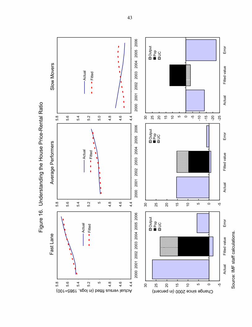
43
Fi
gure
16.
Und
erst
andi
ng th
e H
ouse
Pric
e-R
enta
l Rat
io
Sour
ce: I
MF
staf
f cal
cula
tions
.
4.4
4.6
4.85
5.2
5.4
5.6
5.8
2000
2001
2002
2003
2004
2005
2006
Actual versus fitted (in logs, 1985=100)
Act
ual
Fitte
d
4.4
4.6
4.85
5.2
5.4
5.6
5.8
2000
2001
2002
2003
2004
2005
2006
Act
ual
Fitte
d
4.4
4.6
4.8
5.0
5.2
5.4
5.6
5.8
2000
2001
2002
2003
2004
2005
2006
Act
ual
Fitte
d
-5051015202530
Act
ual
Fitte
d va
lue
Erro
r
Change since 2000 (in percent)
Out
put
Pop
UC
-5051015202530
Act
ual
Fitte
d va
lue
Erro
r
Out
put
Pop
UC
-25
-20
-15
-10-5051015202530
Act
ual
Fitte
d va
lue
Erro
r
Out
put
Pop
UC
Fast
Lan
eAv
erag
e P
erfo
rmer
sSl
ow M
over
s
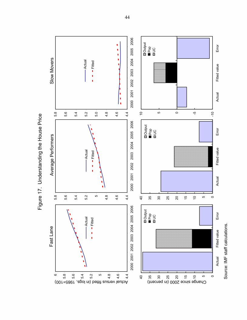
44
Figu
re 1
7. U
nder
stan
ding
the
Hou
se P
rice
Sour
ce: I
MF
staf
f cal
cula
tions
.
4.4
4.6
4.85
5.2
5.4
5.6
5.86
2000
2001
2002
2003
2004
2005
2006
Actual versus fitted (in logs, 1985=100)
Act
ual
Fitte
d
4.4
4.6
4.85
5.2
5.4
5.6
5.8
2000
2001
2002
2003
2004
2005
2006
Act
ual
Fitte
d
4.4
4.6
4.8
5.0
5.2
5.4
5.6
5.8
2000
2001
2002
2003
2004
2005
2006
Act
ual
Fitte
d
0510152025303540
Act
ual
Fitte
d va
lue
Erro
r
Change since 2000 (in percent)
Out
put
Pop
UC
0510152025303540
Act
ual
Fitte
d va
lue
Erro
r
Out
put
Pop
UC
-10-50510
Act
ual
Fitte
d va
lue
Err
or
Out
put
Pop
UC
Fast
Lan
eAv
erag
e Pe
rform
ers
Slow
Mov
ers
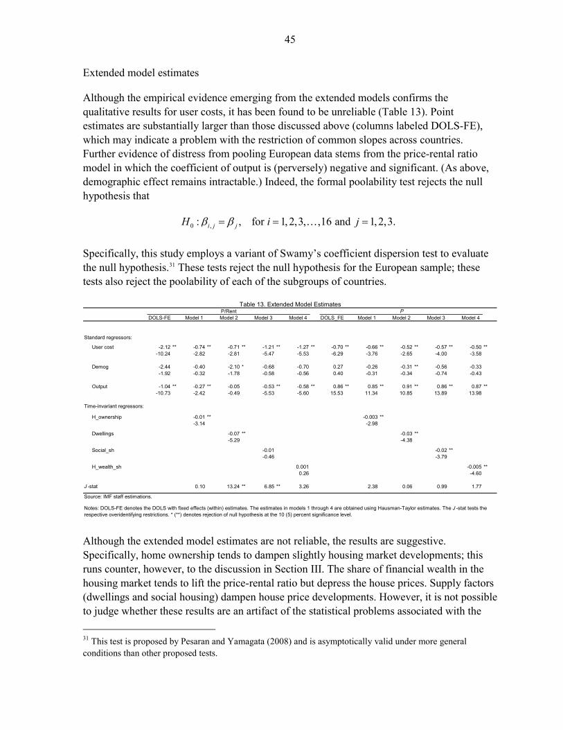
45
Extended model estimates
Although the empirical evidence emerging from the extended models confirms the qualitative results for user costs, it has been found to be unreliable (Table 13). Point estimates are substantially larger than those discussed above (columns labeled DOLS-FE), which may indicate a problem with the restriction of common slopes across countries. Further evidence of distress from pooling European data stems from the price-rental ratio model in which the coefficient of output is (perversely) negative and significant. (As above, demographic effect remains intractable.) Indeed, the formal poolability test rejects the null hypothesis that
0 ,: , for 1, 2,3, ,16 and 1,2,3. i j jH i jβ β= = =…
Specifically, this study employs a variant of Swamy’s coefficient dispersion test to evaluate the null hypothesis.31 These tests reject the null hypothesis for the European sample; these tests also reject the poolability of each of the subgroups of countries.
DOLS-FE Model 1 Model 2 Model 3 Model 4 DOLS_FE Model 1 Model 2 Model 3 Model 4
Standard regressors:
User cost -2.12 ** -0.74 ** -0.71 ** -1.21 ** -1.27 ** -0.70 ** -0.66 ** -0.52 ** -0.57 ** -0.50 **-10.24 -2.82 -2.81 -5.47 -5.53 -6.29 -3.76 -2.65 -4.00 -3.58
Demog -2.44 -0.40 -2.10 * -0.68 -0.70 0.27 -0.26 -0.31 ** -0.56 -0.33-1.92 -0.32 -1.78 -0.58 -0.56 0.40 -0.31 -0.34 -0.74 -0.43
Output -1.04 ** -0.27 ** -0.05 -0.53 ** -0.58 ** 0.86 ** 0.85 ** 0.91 ** 0.86 ** 0.87 **-10.73 -2.42 -0.49 -5.53 -5.60 15.53 11.34 10.85 13.89 13.98
Time-invariant regressors:
H_ownership -0.01 ** -0.003 **-3.14 -2.98
Dwellings -0.07 ** -0.03 **-5.29 -4.38
Social_sh -0.01 -0.02 **-0.46 -3.79
H_wealth_sh 0.001 -0.005 **0.26 -4.60
J -stat 0.10 13.24 ** 6.85 ** 3.26 2.38 0.06 0.99 1.77
Table 13. Extended Model Estimates
Notes: DOLS-FE denotes the DOLS with fixed effects (within) estimates. The estimates in models 1 through 4 are obtained using Hausman-Taylor estimates. The J -stat tests the respective overidentifying restrictions. * (**) denotes rejection of null hypothesis at the 10 (5) percent significance level.
Source: IMF staff estimations.
P/Rent P
Although the extended model estimates are not reliable, the results are suggestive. Specifically, home ownership tends to dampen slightly housing market developments; this runs counter, however, to the discussion in Section III. The share of financial wealth in the housing market tends to lift the price-rental ratio but depress the house prices. Supply factors (dwellings and social housing) dampen house price developments. However, it is not possible to judge whether these results are an artifact of the statistical problems associated with the 31 This test is proposed by Pesaran and Yamagata (2008) and is asymptotically valid under more general conditions than other proposed tests.
46
pooled data or reflect underlying economic relationships. The discussion below thus relies on estimates of the standard model.
Rising interest rates and valuation assessments
Higher interest rates generate overvaluation by increasing user costs. As user costs rise, prices decline in the long run and thus generate overvaluation today. As discussed above, this
leads mechanically to an overvaluation equal to ( )( )
,1 , iˆ .i i tuc ucβ−
⋅ − Measuring this effect,
however, requires not only estimating the ,1iβ but also assessing how the user cost responds
to changes in the real interest rates, namely, / .RFuc r∂ ∂ A simple way to assess this response is to estimate the following model:
, 1, ,
, 0, , ,
RFi t i i t
i t i i t
uc rφ η
η φ ξ
= ⋅ +
= +
where iφ captures cross-country differences in the user cost level and ,i tξ is an error term
with the usual properties.32 The 1,iφ approximates / RFuc r∂ ∂ :
( ) ( )1, , ,1 1 1 0,m
PIT gi ii i t i tRF RF
r gr r
φ τ τ⎡ ⎤∂ ∂
≈ + − ⋅ − − ⋅ >⎢ ⎥∂ ∂⎣ ⎦
where the first term in brackets, as discussed above, represents the common opportunity cost of alternative investments, and the other two terms reflect the net increase in mortgage costs
and the impact of interest rates on expected capital gains, where 0iRF
gr∂
<∂
. In other words,
1,iφ contains a common part (the opportunity cost of investing in housing markets) and country-specific parts (reflecting the tax code, the financial system, and expected capital gains).
Increases in interest rates translate into user costs increases that are about a third as large. Using the panel estimation technique employed above results in an estimate of about 1.3 for
1φ (Table 14).33 This suggests that the country-specific impact—net mortgage costs and net
32 In essence, this specification characterizes user costs as a two-way error component model, with heterogeneous slope coefficients.
33 It is greater than one because the movements in interest rates are smaller compared to those in user costs, as noted in the discussion of partial user cost measures above.
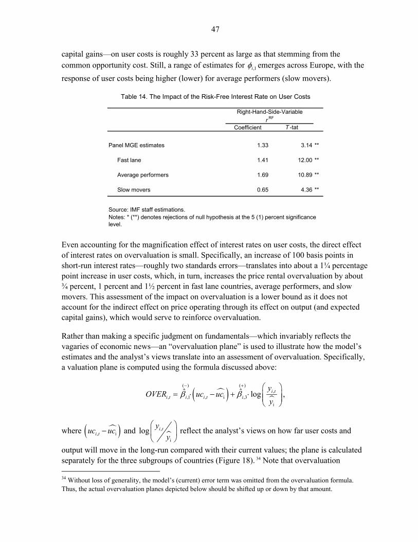
47
capital gains—on user costs is roughly 33 percent as large as that stemming from the common opportunity cost. Still, a range of estimates for ,1iφ emerges across Europe, with the response of user costs being higher (lower) for average performers (slow movers).
Coefficient T -tat
Panel MGE estimates 1.33 3.14 **
Fast lane 1.41 12.00 **
Average performers 1.69 10.89 **
Slow movers 0.65 4.36 **
Source: IMF staff estimations.
Table 14. The Impact of the Risk-Free Interest Rate on User Costs
Notes: * (**) denotes rejections of null hypothesis at the 5 (1) percent significance level.
r RFRight-Hand-Side-Variable
Even accounting for the magnification effect of interest rates on user costs, the direct effect of interest rates on overvaluation is small. Specifically, an increase of 100 basis points in short-run interest rates—roughly two standards errors—translates into about a 1¼ percentage point increase in user costs, which, in turn, increases the price rental overvaluation by about ¾ percent, 1 percent and 1½ percent in fast lane countries, average performers, and slow movers. This assessment of the impact on overvaluation is a lower bound as it does not account for the indirect effect on price operating through its effect on output (and expected capital gains), which would serve to reinforce overvaluation.
Rather than making a specific judgment on fundamentals—which invariably reflects the vagaries of economic news—an “overvaluation plane” is used to illustrate how the model’s estimates and the analyst’s views translate into an assessment of overvaluation. Specifically, a valuation plane is computed using the formula discussed above:
( )( ) ( )
,, ,1 , i ,3
i
ˆ ˆ log ,i ti t i i t i
yOVER uc uc
yβ β− + ⎛ ⎞
= ⋅ − + ⋅ ⎜ ⎟⎜ ⎟⎝ ⎠
where ( ) ,, i
i
and log i ti t
yuc ucy
⎛ ⎞− ⎜ ⎟
⎝ ⎠reflect the analyst’s views on how far user costs and
output will move in the long-run compared with their current values; the plane is calculated separately for the three subgroups of countries (Figure 18). 34 Note that overvaluation 34 Without loss of generality, the model’s (current) error term was omitted from the overvaluation formula. Thus, the actual overvaluation planes depicted below should be shifted up or down by that amount.
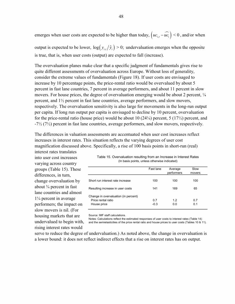
48
emerges when user costs are expected to be higher than today, ( ), i < 0 ,i tuc uc− and/or when
output is expected to be lower, ( ), ˆlog > 0;i t iy y undervaluation emerges when the opposite
is true, that is, when user costs (output) are expected to fall (increase).
The overvaluation planes make clear that a specific judgment of fundamentals gives rise to quite different assessments of overvaluation across Europe. Without loss of generality, consider the extreme values of fundamentals (Figure 18). If user costs are envisaged to increase by 10 percentage points, the price-rental ratio would be overvalued by about 5 percent in fast lane countries, 7 percent in average performers, and about 11 percent in slow movers. For house prices, the degree of overvaluation emerging would be about 2 percent, ¼ percent, and 1½ percent in fast lane countries, average performers, and slow movers, respectively. The overvaluation sensitivity is also large for movements in the long-run output per capita. If long run output per capita is envisaged to decline by 10 percent, overvaluation for the price-rental ratio (house price) would be about 10 (24¼) percent, 5 (17½) percent, and -7½ (7½) percent in fast lane countries, average performers, and slow movers, respectively.
The differences in valuation assessments are accentuated when user cost increases reflect increases in interest rates. This situation reflects the varying degrees of user cost magnification discussed above. Specifically, a rise of 100 basis points in short-run (real) interest rates translates into user cost increases varying across country groups (Table 15). These differences, in turn, change overvaluation by about ¾ percent in fast lane countries and almost 1¼ percent in average performers; the impact on slow movers is nil. (For housing markets that are undervalued to begin with, rising interest rates would serve to reduce the degree of undervaluation.) As noted above, the change in overvaluation is a lower bound: it does not reflect indirect effects that a rise on interest rates has on output.
Fast lane Average Slowperformers movers
Short run interest rate increase 100 100 100
Resulting increase in user costs 141 169 65
Change in overvaluation (in percent)Price rental ratio 0.7 1.2 0.7House price -0.3 0.0 0.1
Source: IMF staff calculations.
Table 15. Overvaluation resulting from an Increase in Interest Rates(In basis points, unless otherwise indicated)
Notes: Calculations reflect the estimated responses of user costs to interest rates (Table 14) and the semielasticities of the price rental ratio and house prices to user costs (Tables 10 & 11).
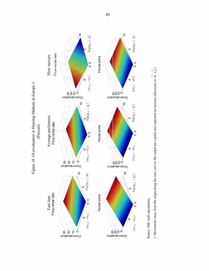
49
Fig
ure
18. O
verv
alua
tion
in H
ousin
g M
arke
ts in
Eur
ope
1/
(Per
cent
)
F
ast l
ane
Ave
rage
per
form
ers
Slo
w m
over
s
So
urce
: IM
F sta
ff ca
lcul
atio
ns.
1/ M
ovem
ents
away
from
the
orig
in a
long
the
user
cos
t (or
the
outp
ut p
er c
apita
) axi
s rep
rese
nt a
n in
crea
se (d
ecre
ase)
in
ii
().
ucy

50
V. SUMMARY AND CONCLUDING REMARKS
The unique features of housing markets complicate assessments of price developments. The heterogeneity of the product in terms of quality, size and location makes the compilation of reliable price indices and, thereby, the identification and interpretation of price developments often difficult. In addition, there are data limitations regarding the factors determining demand and supply. This paper identifies and provides guidance on the key aspects and indicators necessary to assess conditions in housing markets.
The objective is to find out what drives house prices in Europe, and explain the large intra-European differences by distinguishing three groups of advanced economies: (i) fast lane countries—Spain, Ireland, Belgium, the Netherlands, the United Kingdom and France—which until recently experienced very rapid increases in house prices; (ii) average performers—comprising the Nordic countries, Italy and Greece—which witnessed less dramatic but still significant real price increases over the past two decades; and (iii) relatively slow movers—Austria, Germany, Switzerland and Portugal—which stand out the most, with hardly any increase in real house prices.
The study casts a wide net of potential indicators that could help understand housing market developments, including key demand factors such as income, interest rates, and demographics; supply conditions; taxation; and housing finance options. User costs—the total annual cost of home ownership, which lies at the heart of conceptual models of housing markets—were measured and found, until recently, to have declined. Most of the user cost declines were associated with drops in interest rates coupled with (expected) capital gains. However, as interest rates went up and house price increases slowed, user costs have risen markedly since 2006, eroding much of the earlier decline.
The empirical evidence suggests that the standard model—combining user costs, demographic factors and output—fits most of the countries well and points to the differing responsiveness of house prices within Europe. House prices are, as expected, inversely related to user costs and directly linked to output. Demographic factors were not found to be robustly related to house price developments over the 20-year sample period, although since the beginning of this decade the correlation seems to have strengthened. House price developments in fast lane countries appear to be more responsive to income developments than in average performers, which in turn are more sensitive than slow movers. Although the bulk of the movements in house prices projected by the model are associated with output developments, this may overstate (understate) the importance of output (user costs) as the intrinsic effect is not separated from the movement in output in response to changes in the interest rate.
The standard model captures housing market developments in the fast lane and among average performers relatively well. Still, the model underpredicts observed prices in these countries toward the end of the sample period. Assessing the degree to which housing market developments imply overvaluation would require taking a stance on the value of fundamentals in the long run, including hard-to-quantify supply factors not included in the model. Nevertheless, the sensitivity of prices uncovered in the fast lane countries and, to a somewhat lesser extent, the average performers
51
suggests that these countries can face greater challenges following adverse developments in fundamentals.
Consistent with the stylized facts, house price developments in slow movers are harder to explain with the standard set of fundamentals. In part, this may reflect that estimates are based on a smaller sample than those from the other groups. Efforts to better understand housing market developments —extending the set of fundamentals considered in the model—were thwarted by the “snapshot” nature of the available data. The restrictions needed to measure the effects of time-invariant fundamentals were rejected by the data. Nevertheless, ample supply, low home ownership levels and less complete mortgage markets are likely contributing factors to developments in slow movers.
While not the main focus of the study, a few general observations about policy implications are worth making:
• The impact of monetary policy is amplified by its impact on house prices, which differs across Europe. In particular, this effect is more pronounced in the fast lane countries, where house prices have been found to be more sensitive to output and interest rate developments. Of relevance for countries in the euro area is a lack of a uniform reaction to interest rate changes in the various national housing markets.
• Fiscal policy affects house prices largely through taxes and subsidies. Accounting for their impact on the housing market, and thereby on the economy, should be an integral part of assessing the desirability of such policies. Experiences in some countries have shown that gradual changes in housing taxation, in particular when announced well in advance, can help avoid abrupt price movements.
• Structural policies can have a substantial impact on the supply side of the market. Policies affecting the construction industry and building (zoning) regulations affect house prices through their impact on supply. Supply rigidities are a common phenomenon in Europe, and can explain to some degree the until recently sharp price increases in certain countries.
• The study also points to the relevance of financial sector policies for developments in the housing market. More complete mortgage markets with enhanced financing options will stimulate the market, but can also contribute to risks and unbalanced developments. Effective regulatory oversight and supervision of the (mortgage) banking industry is key to limiting the vulnerabilities in housing markets.
In sum, given (i) the increased importance of housing markets for macroeconomic and financial stability; (ii) the historically high real house prices in many European countries and the recent turn in the markets in some of the fast lane countries, where house prices appear most sensitive to fundamentals; and (iii) the significant impact of monetary, taxation, structural and prudential policies on house price developments in Europe, careful consideration of the implications of economic policies on the stability of housing markets is warranted.
52
REFERENCES
Abiad, A, and A. Mody, 2003, “Financial Reform: What Shakes It? What Shapes It?” IMF Working Paper 03/70 (Washington: International Monetary Fund).
Allen, M., C. Rosenberg, C. Keller, B. Setser, and N. Roubini, 2002, “A Balance Sheet Approach to Financial Crisis,” IMF Working Paper 02/210 (Washington: International Monetary Fund).
Ayuso, Juan, and Fernando Restoy, 2003, “House Prices and Rents: An Equilibrium Asset Price Approach,” Bank of Spain, Working Paper No. 0304 (Madrid: Bank of Spain).
Bank for International Settlements, 2005, “Real Estate Indicators and Financial Stability,” BIS Papers, No. 21 (Basel: Bank for International Settlements).
Bernanke, B., and S. Gilchrist, 1999, “The Financial Accelerator in a Quantitative Business Cycle Framework,” in Handbook of Macroeconomics, Vol. 1C, ed. by J. Taylor and M. Woolford (Amsterdam: North-Holland).
Boone, L., N. Girouard, and I. Wanner, 2001, “Financial Market Liberalisation, Wealth and Consumption,” OECD Economics Department Working Papers, No. 308 (Paris: OECD).
Catte, P., N. Girouard, R. Price, and C. André, 2004, “Housing Markets, Wealth and the Business Cycle,” OECD Economics Department Working Papers, No. 394 (Paris: OECD).
Collyns, C., and A. Senhadji, 2002, “Lending Booms, Real Estate Bubbles and the Asian Crisis,” IMF Working Paper 02/20 (Washington: International Monetary Fund).
Committee on the Global Financial System, 2006, “Housing Finance in the Global Financial Market,” CGFS Papers, No. 26 (Basel: Bank for International Settlements).
Cournède, B., 2005, “House Prices and Inflation in the Euro Area,” OECD Economics Department Working Papers, No. 450 (Paris: OECD).
Decressin, J., H. Faruqee, and W. Fonteyne, 2007, eds., Integrating Europe’s Financial Markets, (Washington: International Monetary Fund).
Egert, B., and D. Mihaljek, 2007, “Determinants of House Price Dynamics in Central and Eastern Europe,” in Focus on European Economic Integration 1/07 (Vienna: Austrian National Bank).
Engel, R., and C. Granger, 1987, “Co-integration and Error Correction: Representation, Estimation, and Testing,” Econometrica, Vol. 55, pp. 251–76.
European Central Bank, 2003, “Structural Factors in the EU Housing Markets” (Frankfurt: European Central Bank).
———, 2007a, Monthly Bulletin, September (Frankfurt: European Central Bank).
———, 2007b, Financial Stability Review, December (Frankfurt: European Central Bank).
53
European Commission, 2005, “Green Paper: Mortgage Credit in the EU” (Brussels: Commission of the European Communities).
European Commission, 2008, EMU@10: Successes and Challenges after 10 Years of Economic and Monetary Union (Brussels: Commission of the European Communities).
European Mortgage Federation, 2004, A Review of Europe’s Mortgage and Housing Markets (Brussels: European Mortgage Federation).
———, 2006a, Hypostat (Brussels: European Mortgage Federation).
———, 2006b, Study on Interest Rate Variability in Europe (Brussels: European Mortgage Federation).
———, 2006c, Study on the Cost of Housing in Europe (Brussels: European Mortgage Federation).
Garber, P., 2001, Famous First Bubbles (Cambridge, Massachusetts: MIT Press).
Girouard, N., M. Kennedy, P. van den Noord, and C. André, 2006, “Recent House Price Developments: The Role of Fundamentals,” OECD Economics Department Working Paper No. 475 (Paris: OECD).
Hilbers, P., Q. Lei, and L. Zacho, 2001, “Real Estate Developments and Financial Sector Soundness,” IMF Working Paper 01/129 (Washington: International Monetary Fund).
Hausman, J.A., and W.E. Taylor, 1981, “Panel Data and Unobservable Individual Effects,” Econometrica, Vol. 49, No. 6, pp. 1377–98.
Himmelberg, C., C. Mayer, and T. Sinai, 2005, “Assessing High House Prices: Bubbles, Fundamentals, and Misperceptions,” Journal of Economic Perspectives, Vol. 19, No. 4, pp. 67–92.
International Bureau of Fiscal Documentation, European Tax Handbook (Amsterdam, Netherlands), various annual issues.
International Monetary Fund, 2005, Global Financial Stability Report, April.
———, 2008a, World Economic Outlook, April 2008 (Washington: International Monetary Fund).
———, 2008b, Regional Economic Outlook: Europe, April (Washington: International Monetary Fund).
Johansen, S., 1988, “Statistical Analysis of Cointegrating Vectors,” Journal of Economic Dynamics and Control, Vol. 12, Nos. 2-3, pp. 231–54.
———, 1991, “Estimation and Hypothesis Testing of Cointegrating Vectors in Gaussian Vector Autoregressive Models,” Econometrica, No. 6, Vol. 59, pp. 1551–80.
Kiyotaki, N., and J. Moore, 1997, “Credit Cycles,” Journal of Political Economy, Vol. 105, pp. 211-48.
Mercer Oliver Wyman, 2003, Study on the Financial Integration of the European Mortgage Markets (Brussels: European Mortgage Federation).
54
Muellbauer, J., and A. Murphy, 1997, “Booms and Busts in the UK Housing Market,” Economic Journal, No. 107 (November), pp. 1701-27.
Odenius, J., A. Carare, and E. Crivelli, 2008, “No Boom No Bust—Germany’s Lackluster Real Estate Market” (unpublished; Washington: International Monetary Fund).
Organization for Economic Cooperation and Development, 2007, Revenue Statistics 1965–2006 (Paris: OECD).
Pesaran, M.H., and R. Smith, 1995, “Estimating Long-Run Relationships From Dynamic Heterogeneous Panels,” Journal of Econometrics, Vol. 68 (July), pp. 79–113.
Pesaran, M.H., and T. Yamagata, 2008, “Testing Slope Homogeneity in Large Panels,” Journal of Econometrics, Vol. 142 (January), pp. 50–93.
Pedroni, P., 2001, “Purchasing Power Parity Test in Cointegrated Panels,” Review of Economics and Statistics, Vol. 83, No. 4, pp. 727–31.
Poterba, J., 1984, “Tax Subsidies to Owner-Occupied Housing: An Asset-Market Approach,” The Quarterly Journal of Economics, Vol. 99, No. 4, pp. 729–52.
———, 1991, “House Price Dynamics: The Role of Tax Policy and Demography,” Brooking Papers on Economic Activity: 2, Brookings Institution , pp. 143–203.
Sorensen, C., and J. Lichtenberger, 2007, “Mortgage Interest Dispersion in the Euro Area,” ECB Working Paper No. 733 (Frankfurt: European Central Bank).
Stock, J., and M. Watson, 1993, “A Simple Estimator of Cointegrating Vectors in Higher-Order Integrated Systems,” Econometrica, Vol. 61, No. 4, pp. 783–820.
Terrones, M., and C. Otrok, 2004, “The Global House Price Boom,” in World Economic Outlook September 2004 (Washington: International Monetary Fund), pp. 71-89.
Yelten, S., 2006, “Determinants, Concerns, and Considerations Related to Phasing Out the Tax Deductibility of Mortgage Interest Payments,” in Kingdom of the Netherlands— Selected Issues, Country Report 06/284 (Washington: International Monetary Fund).
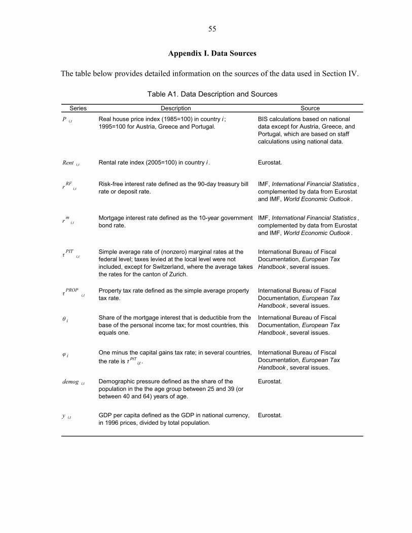
55
Appendix I. Data Sources The table below provides detailed information on the sources of the data used in Section IV.
Series Description Source
P i,t Real house price index (1985=100) in country i ; 1995=100 for Austria, Greece and Portugal.
BIS calculations based on national data except for Austria, Greece, and Portugal, which are based on staff calculations using national data.
Rent i,t Rental rate index (2005=100) in country i . Eurostat.
r RFi,t
Risk-free interest rate defined as the 90-day treasury bill rate or deposit rate.
IMF, International Financial Statistics , complemented by data from Eurostat and IMF, World Economic Outlook .
r mi,t
Mortgage interest rate defined as the 10-year government bond rate.
IMF, International Financial Statistics , complemented by data from Eurostat and IMF, World Economic Outlook .
τ PIT i,t
Simple average rate of (nonzero) marginal rates at the federal level; taxes levied at the local level were not included, except for Switzerland, where the average takes the rates for the canton of Zurich.
International Bureau of Fiscal Documentation, European Tax Handbook , several issues.
τ PROP i,t
Property tax rate defined as the simple average property tax rate.
International Bureau of Fiscal Documentation, European Tax Handbook , several issues.
θ i Share of the mortgage interest that is deductible from the base of the personal income tax; for most countries, this equals one.
International Bureau of Fiscal Documentation, European Tax Handbook , several issues.
φ i One minus the capital gains tax rate; in several countries, the rate is τ PIT
i,t .International Bureau of Fiscal Documentation, European Tax Handbook , several issues.
demog i,t Demographic pressure defined as the share of the population in the the age group between 25 and 39 (or between 40 and 64) years of age.
Eurostat.
y i,t GDP per capita defined as the GDP in national currency, in 1996 prices, divided by total population.
Eurostat.
Table A1. Data Description and Sources

56
Appendix II. Housing-Related Taxation
This appendix provides details about the variety of housing tax regimes in the various countries under consideration, including about relevant rates, the taxable base, and exemptions and deductions.35
A. Personal Income Tax (PIT) Rates
Important factors determining the effect of PIT on the housing market are:
• Deductibility of mortgage interest payments or other housing related costs from taxable income. In many countries mortgage interest is either deductible from taxable income or partly refunded to the taxpayers; however, this is typically subject to restrictions and limits (Table A2). In Austria, Belgium, Sweden, and Switzerland, taxpayers can deduct their mortgage payments up to a ceiling. Ireland, Portugal, and Spain refund part of the mortgage interest to the taxpayers, but again subject to maximum amounts. Italy and Greece switched from a policy of full mortgage interest deduction to one of granting refunds only for mortgage interest payments on principal homes. France and the United Kingdom ended mortgage interest refunds in 1998 and 1999, respectively, but France re-introduced it in 2007. Mortgage interest is not deductible from taxable income in Germany.
• Deductibility of property tax from rental income. Property tax is deductible from rental income for all countries that have such a tax.
B. (Imputed) Rental Income Tax
Net rental income (surplus of receipts over expenses) is taxable income in all countries, but sometimes subject to exemptions (Table A3). Ireland, Norway, Sweden, and the United Kingdom apply either standard deductions or exemptions for rental income. In Spain, rental properties are taxed on imputed income or actual rental income (if the latter, only 50 percent of the rental income is taxable). Rental income is usually taxed at the personal income tax rate, except in Greece and Sweden. In Greece, an additional 1.5 percent surtax is levied on the rental income. In Sweden, rental income is taxed as capital income at a flat rate of 30 percent.
35 The information on housing related taxation is mostly taken from the 2005 European Tax Handbook. Recent updates in some of the national tax codes are not represented here.
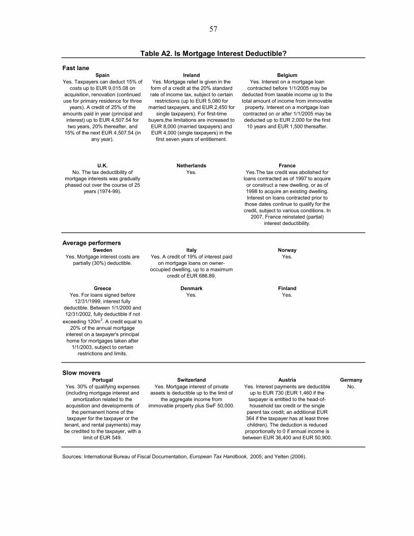
57
Fast laneSpain Ireland Belgium
Yes. Taxpayers can deduct 15% of costs up to EUR 9,015.08 on
acquisition, renovation (continued use for primary residence for three
years). A credit of 25% of the amounts paid in year (principal and
interest) up to EUR 4,507.54 for two years, 20% thereafter, and
15% of the next EUR 4,507.54 (in any year).
Yes. Mortgage relief is given in the form of a credit at the 20% standard rate of income tax, subject to certain
restrictions (up to EUR 5,080 for married taxpayers, and EUR 2,450 for
single taxpayers). For first-time buyers,the limitations are increased to EUR 8,000 (married taxpayers) and EUR 4,000 (single taxpayers) in the
first seven years of entitlement.
Yes. Interest on a mortgage loan contracted before 1/1/2005 may be
deducted from taxable income up to the total amount of income from immovable
property. Interest on a mortgage loan contracted on or after 1/1/2005 may be deducted up to EUR 2,000 for the first 10 years and EUR 1,500 thereafter.
U.K. Netherlands FranceNo. The tax deductibility of
mortgage interests was gradually phased out over the course of 25
years (1974-99).
Yes. Yes.The tax credit was abolished for loans contracted as of 1997 to acquire or construct a new dwelling, or as of 1998 to acquire an existing dwelling. Interest on loans contracted prior to
those dates continue to qualify for the credit, subject to various conditions. In
2007, France reinstated (partial) interest deductibility.
Average performersSweden Italy Norway
Yes. Mortgage interest costs are partially (30%) deductible.
Yes. A credit of 19% of interest paid on mortgage loans on owner-
occupied dwelling, up to a maximum credit of EUR 686.89.
Yes.
Greece Denmark FinlandYes. For loans signed before
12/31/1999, interest fully deductible. Between 1/1/2000 and 12/31/2002, fully deductible if not
exceeding 120m2. A credit equal to 20% of the annual mortgage
interest on a taxpayer's principal home for mortgages taken after
1/1/2003, subject to certain restrictions and limits.
Yes. Yes.
Slow moversPortugal Switzerland Austria Germany
Yes. 30% of qualifying expenses (including mortgage interest and
amortization related to the acquisition and developments of
the permanent home of the taxpayer for the taxpayer or the
tenant, and rental payments) may be credited to the taxpayer, with a
limit of EUR 549.
Yes. Mortgage interest of private assets is deductible up to the limit of
the aggregate income from immovable property plus SwF 50,000.
Yes. Interest payments are deductible up to EUR 730 (EUR 1,460 if the
taxpayer is entitled to the head-of-household tax credit or the single
parent tax credit; an additional EUR 364 if the taxpayer has at least three children). The deduction is reduced
proportionally to 0 if annual income is between EUR 36,400 and EUR 50,900.
No.
Sources: International Bureau of Fiscal Documentation, European Tax Handbook, 2005; and Yelten (2006).
Table A2. Is Mortgage Interest Deductible?
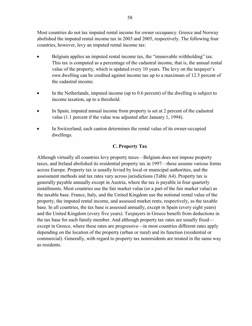
58
Most countries do not tax imputed rental income for owner occupancy. Greece and Norway abolished the imputed rental income tax in 2003 and 2005, respectively. The following four countries, however, levy an imputed rental income tax:
• Belgium applies an imputed rental income tax, the “immovable withholding” tax. This tax is computed as a percentage of the cadastral income, that is, the annual rental value of the property, which is updated every 10 years. The levy on the taxpayer’s own dwelling can be credited against income tax up to a maximum of 12.5 percent of the cadastral income.
• In the Netherlands, imputed income (up to 0.6 percent) of the dwelling is subject to income taxation, up to a threshold.
• In Spain, imputed annual income from property is set at 2 percent of the cadastral value (1.1 percent if the value was adjusted after January 1, 1994).
• In Switzerland, each canton determines the rental value of its owner-occupied dwellings.
C. Property Tax
Although virtually all countries levy property taxes—Belgium does not impose property taxes, and Ireland abolished its residential property tax in 1997—these assume various forms across Europe. Property tax is usually levied by local or municipal authorities, and the assessment methods and tax rates vary across jurisdictions (Table A4). Property tax is generally payable annually except in Austria, where the tax is payable in four quarterly installments. Most countries use the fair market value (or a part of the fair market value) as the taxable base. France, Italy, and the United Kingdom use the notional rental value of the property, the imputed rental income, and assessed market rents, respectively, as the taxable base. In all countries, the tax base is assessed annually, except in Spain (every eight years) and the United Kingdom (every five years). Taxpayers in Greece benefit from deductions in the tax base for each family member. And although property tax rates are usually fixed—except in Greece, where these rates are progressive—in most countries different rates apply depending on the location of the property (urban or rural) and its function (residential or commercial). Generally, with regard to property tax nonresidents are treated in the same way as residents.
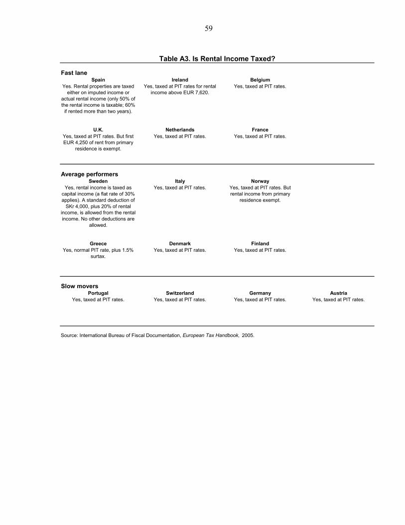
59
Fast laneSpain Ireland Belgium
Yes. Rental properties are taxed either on imputed income or
actual rental income (only 50% of the rental income is taxable; 60%
if rented more than two years).
Yes, taxed at PIT rates for rental income above EUR 7,620.
Yes, taxed at PIT rates.
U.K. Netherlands FranceYes, taxed at PIT rates. But first EUR 4,250 of rent from primary
residence is exempt.
Yes, taxed at PIT rates. Yes, taxed at PIT rates.
Average performersSweden Italy Norway
Yes, rental income is taxed as capital income (a flat rate of 30% applies). A standard deduction of
SKr 4,000, plus 20% of rental income, is allowed from the rental income. No other deductions are
allowed.
Yes, taxed at PIT rates. Yes, taxed at PIT rates. But rental income from primary
residence exempt.
Greece Denmark FinlandYes, normal PIT rate, plus 1.5%
surtax.Yes, taxed at PIT rates. Yes, taxed at PIT rates.
Slow moversPortugal Switzerland Germany Austria
Yes, taxed at PIT rates. Yes, taxed at PIT rates. Yes, taxed at PIT rates. Yes, taxed at PIT rates.
Source: International Bureau of Fiscal Documentation, European Tax Handbook, 2005.
Table A3. Is Rental Income Taxed?
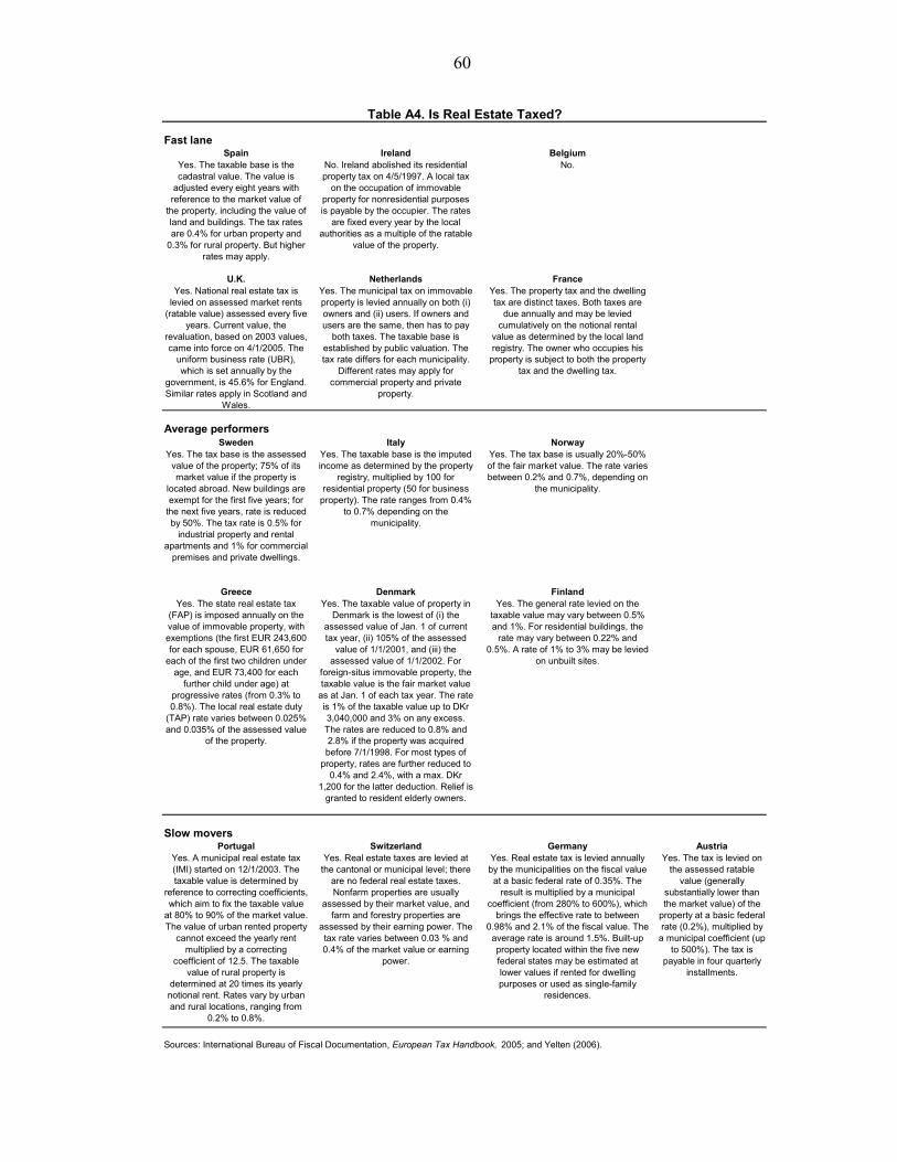
60
Fast laneSpain Ireland Belgium
Yes. The taxable base is the cadastral value. The value is
adjusted every eight years with reference to the market value of
the property, including the value of land and buildings. The tax rates are 0.4% for urban property and
0.3% for rural property. But higher rates may apply.
No. Ireland abolished its residential property tax on 4/5/1997. A local tax
on the occupation of immovable property for nonresidential purposes is payable by the occupier. The rates
are fixed every year by the local authorities as a multiple of the ratable
value of the property.
No.
U.K. Netherlands FranceYes. National real estate tax is
levied on assessed market rents (ratable value) assessed every five
years. Current value, the revaluation, based on 2003 values, came into force on 4/1/2005. The
uniform business rate (UBR), which is set annually by the
government, is 45.6% for England. Similar rates apply in Scotland and
Wales.
Yes. The municipal tax on immovable property is levied annually on both (i) owners and (ii) users. If owners and users are the same, then has to pay
both taxes. The taxable base is established by public valuation. The tax rate differs for each municipality.
Different rates may apply for commercial property and private
property.
Yes. The property tax and the dwelling tax are distinct taxes. Both taxes are
due annually and may be levied cumulatively on the notional rental
value as determined by the local land registry. The owner who occupies his
property is subject to both the property tax and the dwelling tax.
Average performersSweden Italy Norway
Yes. The tax base is the assessed value of the property; 75% of its market value if the property is
located abroad. New buildings are exempt for the first five years; for
the next five years, rate is reduced by 50%. The tax rate is 0.5% for
industrial property and rental apartments and 1% for commercial
premises and private dwellings.
Yes. The taxable base is the imputed income as determined by the property
registry, multiplied by 100 for residential property (50 for business
property). The rate ranges from 0.4% to 0.7% depending on the
municipality.
Yes. The tax base is usually 20%-50% of the fair market value. The rate varies between 0.2% and 0.7%, depending on
the municipality.
Greece Denmark FinlandYes. The state real estate tax
(FAP) is imposed annually on the value of immovable property, with exemptions (the first EUR 243,600 for each spouse, EUR 61,650 for
each of the first two children under age, and EUR 73,400 for each
further child under age) at progressive rates (from 0.3% to 0.8%). The local real estate duty
(TAP) rate varies between 0.025% and 0.035% of the assessed value
of the property.
Yes. The taxable value of property in Denmark is the lowest of (i) the
assessed value of Jan. 1 of current tax year, (ii) 105% of the assessed
value of 1/1/2001, and (iii) the assessed value of 1/1/2002. For
foreign-situs immovable property, the taxable value is the fair market value
as at Jan. 1 of each tax year. The rate is 1% of the taxable value up to DKr 3,040,000 and 3% on any excess. The rates are reduced to 0.8% and 2.8% if the property was acquired before 7/1/1998. For most types of
property, rates are further reduced to 0.4% and 2.4%, with a max. DKr
1,200 for the latter deduction. Relief is granted to resident elderly owners.
Yes. The general rate levied on the taxable value may vary between 0.5% and 1%. For residential buildings, the
rate may vary between 0.22% and 0.5%. A rate of 1% to 3% may be levied
on unbuilt sites.
Slow moversPortugal Switzerland Germany Austria
Yes. A municipal real estate tax (IMI) started on 12/1/2003. The taxable value is determined by
reference to correcting coefficients, which aim to fix the taxable value
at 80% to 90% of the market value. The value of urban rented property
cannot exceed the yearly rent multiplied by a correcting
coefficient of 12.5. The taxable value of rural property is
determined at 20 times its yearly notional rent. Rates vary by urban and rural locations, ranging from
0.2% to 0.8%.
Yes. Real estate taxes are levied at the cantonal or municipal level; there
are no federal real estate taxes. Nonfarm properties are usually
assessed by their market value, and farm and forestry properties are
assessed by their earning power. The tax rate varies between 0.03 % and 0.4% of the market value or earning
power.
Yes. Real estate tax is levied annually by the municipalities on the fiscal value at a basic federal rate of 0.35%. The
result is multiplied by a municipal coefficient (from 280% to 600%), which
brings the effective rate to between 0.98% and 2.1% of the fiscal value. The
average rate is around 1.5%. Built-up property located within the five new federal states may be estimated at lower values if rented for dwelling purposes or used as single-family
residences.
Yes. The tax is levied on the assessed ratable
value (generally substantially lower than the market value) of the
property at a basic federal rate (0.2%), multiplied by
a municipal coefficient (up to 500%). The tax is
payable in four quarterly installments.
Sources: International Bureau of Fiscal Documentation, European Tax Handbook, 2005; and Yelten (2006).
Table A4. Is Real Estate Taxed?

61
D. Capital Gains Tax
Capital gains are taxable in all the countries except Greece and the Netherlands, where even nonresidents are not subject to capital gains tax (Table A5). Most countries include capital gains as part of personal taxable income and thus tax these gains at the income tax rates. However, capital gains in Finland, France, Ireland, Spain, Sweden, and Switzerland are subject to specific capital gains taxes. Switzerland is the only country that levies capital gains progressively.
Many countries provide some sort of capital gains tax relief for owner-occupied properties. Capital gains on owner-occupied properties are exempt from capital gains taxes in Denmark, France, Ireland, Italy, and the United Kingdom. Capital gains tax rates decline with the years of ownership in France, Switzerland, and the United Kingdom. The number of years of ownership needed for full exemption varies from two years in Finland to twenty years in Switzerland. A few countries provide rollover relief.
E. Wealth, Inheritance and Gift Taxes
Most countries do not levy a wealth tax. Austria, Germany, the Netherlands and Sweden abolished their wealth taxes in 1994, 1997, 2001 and 2007, respectively. France, Norway, Spain and Switzerland do impose a tax on wealth (Table A6). Wealth taxes in these countries are generally levied on net wealth above a certain threshold, and the rates are usually progressive.
Inheritances and gifts are taxable in all countries except Italy, Portugal, and Sweden, which abolished these taxes in 2002, 2004, and 2005, respectively (Table A7). Italy imposes a tax on all transfers of immovable properties. Portugal levies a stamp duty on gifts of immovable property if the individual recipient is not related to the deceased/donor. In all other countries, inheritance and gift taxes are levied on the fair market value of the net estate or gift; the rates are usually progressive and typically decline with the ties between the deceased/donor and the heir/donee.

62
Fast laneSpain Ireland Belgium
Yes. But there is rollover relief for capital gains on taxpayer's own
residence. In calculating the capital gains, the acquisition price is
adjusted for inflation. Capital gains derived from a gift to qualifying
donees and capital gains realized by persons 65 years old or older on the sale of their primary residence
are exempt. Capital gains are levied at a flat rate of 15% (9.06%
for the state and 5.94% for the autonomous regions).
Yes. But capital gains realized on the sale of own private residence (and
land up to one acre) are not taxable. The increase in value attributable to the development of the property is
taxable. The ordinary rate of capital gains tax is 20%.
Yes. A rate of 16.5% applies to developed immovable property (33%
for undeveloped property) if sold within five years of acquisition.
U.K. Netherlands FranceYes, with an annual exemption of £ 8,500. But capital gains on primary
residence are exempt, and the percentage of the gains that are taxable declines as the years of
ownership increase. Capital gains tax is levied at the PIT.
No. Capital gains are generally not taxable.
Yes. But gains on the sale of taxpayer's principal residence are exempt from
tax. Gains on any immovable property are exempt if the sales price does not
exceed EUR 15,000. In calculating such gains, the acquisition cost is increased by 15%. The gains so
calculated are further reduced by 10% for each year of ownership beyond the fifth year, which means that gains on
property held for 16 years are exempt. Capital gains are levied at a fixed rate
of 16%.
Average performersSweden Italy Norway
Yes. There is rollover relief. For private dwellings, other than those
qualifying for the tax deferral, including vacation houses, two-
thirds of the capital gains are taxable at a flat rate of 30%.
Yes, if the sale of the immovable property is within five years of
acquisition. But gains on the sale of taxpayer's principal residence are
exempt from tax. Also, capital gains on land and buildings acquired by way of inheritance or donation are exempt.
The capital gains are included in taxable income and levied at the PIT.
Yes. Capital gains are taxable with some exemptions and special
provisions. The capital gains are included in taxable income and levied at the PIT. The general combined rate of the national and municipal income
taxes is 28% (24.5% for Finnmark and Nord-Troms).
Greece Denmark FinlandNo. Capital gains derived from
immovable property are not taxable.
Yes. But gains on the sale of owner-occupied dwellings are normally exempt. The capital gains are
included in taxable income (capital income) and levied at personal
income tax rate.
Yes, if the sale of the immovable property is within two years of
acquisition. The capital gains are levied at a rate of 28%.
Slow moversPortugal Switzerland Germany Austria
Yes. But only 50% of the net capital gains are subject to tax. Acquisition costs are inflation
adjustable after an ownership of two years. There is rollover relief
for taxpayer's permanent dwelling. The capital gains are included in taxable income and levied at the
PIT.
Yes. Capital gains on immovable property located in the canton are
subject to a real estate gains tax. In Zurich, gains of up to SwF 5,000 are exempt. There is rollover relief. The tax rates range from 10% on the first SwF 4,000 to 40% on the excess of
SwF 100,000. The tax is increased by 50% if the ownership is less than one year and by 25% if it is less than two years. The tax is reduced by 5% if
owning is more than five years and is reduced by additional 3% for each
following year. The maximum reduction is 50% if the ownership is
20 years or more.
Yes, if the sale of the immovable property is within 10 years of acquisition
and 50% of the capital gains are exempt from tax. The capital gains are
levied at the normal PIT.
Yes, if the sale of the immovable property is
within 10 years of acquisition. The capital gains are included in
taxable income and levied at the PIT.
Sources: International Bureau of Fiscal Documentation, European Tax Handbook, 2005; and Yelten (2006).
Table A5. Are Capital Gains Taxed?
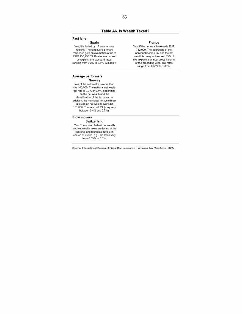
63
Fast laneSpain France
Yes, it is levied by 17 autonomous regions. The taxpayer's primary
residence gets an exemption of up to EUR 150,253.03. If rates are not set
by regions, the standard rates, ranging from 0.2% to 2.5%, will apply.
Yes, if the net wealth exceeds EUR 732,000. The aggregate of the
individual income tax and the net wealth tax may not exceed 85% of the taxpayer's annual gross income
of the preceding year. Tax rates range from 0.55% to 1.80%.
Average performersNorway
Yes, if the net wealth is more than NKr 100,000. The national net wealth tax rate is 0.2% or 0.4%, depending
on the net wealth and the classification of the taxpayer. In
addition, the municipal net wealth tax is levied on net wealth over NKr
151,000. The rate is 0.7% (may vary between 0.4% and 0.7%).
Slow moversSwitzerland
Yes. There is no federal net wealth tax. Net wealth taxes are levied at the
cantonal and municipal levels. In canton of Zurich, e.g., the rates vary
from 0.05% to 0.3%.
Source: International Bureau of Fiscal Documentation, European Tax Handbook, 2005.
Table A6. Is Wealth Taxed?
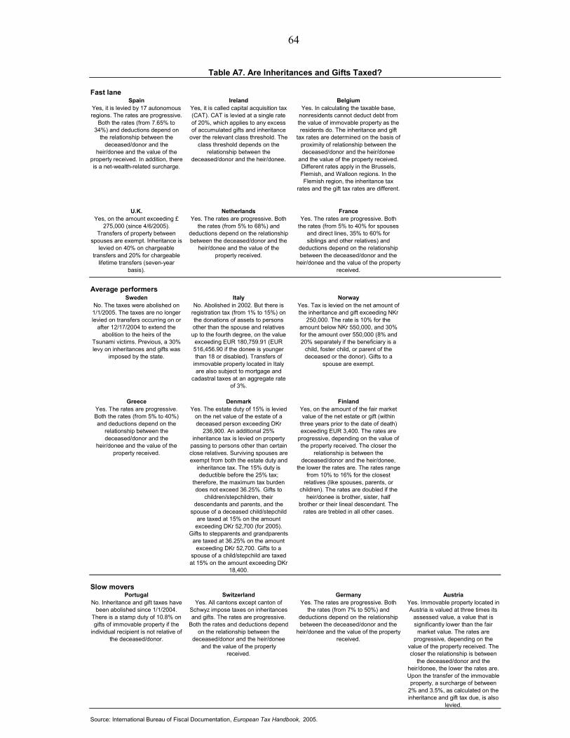
64
Fast laneSpain Ireland Belgium
Yes, it is levied by 17 autonomous regions. The rates are progressive.
Both the rates (from 7.65% to 34%) and deductions depend on
the relationship between the deceased/donor and the
heir/donee and the value of the property received. In addition, there is a net-wealth-related surcharge.
Yes, it is called capital acquisition tax (CAT). CAT is levied at a single rate of 20%, which applies to any excess of accumulated gifts and inheritance
over the relevant class threshold. The class threshold depends on the
relationship between the deceased/donor and the heir/donee.
Yes. In calculating the taxable base, nonresidents cannot deduct debt from the value of immovable property as the residents do. The inheritance and gift
tax rates are determined on the basis of proximity of relationship between the deceased/donor and the heir/donee
and the value of the property received. Different rates apply in the Brussels, Flemish, and Walloon regions. In the Flemish region, the inheritance tax
rates and the gift tax rates are different.
U.K. Netherlands FranceYes, on the amount exceeding £
275,000 (since 4/6/2005). Transfers of property between
spouses are exempt. Inheritance is levied on 40% on chargeable
transfers and 20% for chargeable lifetime transfers (seven-year
basis).
Yes. The rates are progressive. Both the rates (from 5% to 68%) and
deductions depend on the relationship between the deceased/donor and the
heir/donee and the value of the property received.
Yes. The rates are progressive. Both the rates (from 5% to 40% for spouses
and direct lines, 35% to 60% for siblings and other relatives) and
deductions depend on the relationship between the deceased/donor and the
heir/donee and the value of the property received.
Average performersSweden Italy Norway
No. The taxes were abolished on 1/1/2005. The taxes are no longer levied on transfers occurring on or
after 12/17/2004 to extend the abolition to the heirs of the
Tsunami victims. Previous, a 30% levy on inheritances and gifts was
imposed by the state.
No. Abolished in 2002. But there is registration tax (from 1% to 15%) on the donations of assets to persons other than the spouse and relatives up to the fourth degree, on the value
exceeding EUR 180,759.91 (EUR 516,456.90 if the donee is younger than 18 or disabled). Transfers of
immovable property located in Italy are also subject to mortgage and
cadastral taxes at an aggregate rate of 3%.
Yes. Tax is levied on the net amount of the inheritance and gift exceeding NKr
250,000. The rate is 10% for the amount below NKr 550,000, and 30% for the amount over 550,000 (8% and 20% separately if the beneficiary is a
child, foster child, or parent of the deceased or the donor). Gifts to a
spouse are exempt.
Greece Denmark FinlandYes. The rates are progressive. Both the rates (from 5% to 40%) and deductions depend on the
relationship between the deceased/donor and the
heir/donee and the value of the property received.
Yes. The estate duty of 15% is levied on the net value of the estate of a deceased person exceeding DKr
236,900. An additional 25% inheritance tax is levied on property
passing to persons other than certain close relatives. Surviving spouses are exempt from both the estate duty and
inheritance tax. The 15% duty is deductible before the 25% tax;
therefore, the maximum tax burden does not exceed 36.25%. Gifts to
children/stepchildren, their descendants and parents, and the
spouse of a deceased child/stepchild are taxed at 15% on the amount exceeding DKr 52,700 (for 2005).
Gifts to stepparents and grandparents are taxed at 36.25% on the amount
exceeding DKr 52,700. Gifts to a spouse of a child/stepchild are taxed at 15% on the amount exceeding DKr
18,400.
Yes, on the amount of the fair market value of the net estate or gift (within
three years prior to the date of death) exceeding EUR 3,400. The rates are
progressive, depending on the value of the property received. The closer the
relationship is between the deceased/donor and the heir/donee,
the lower the rates are. The rates range from 10% to 16% for the closest
relatives (like spouses, parents, or children). The rates are doubled if the
heir/donee is brother, sister, half brother or their lineal descendant. The
rates are trebled in all other cases.
Slow moversPortugal Switzerland Germany Austria
No. Inheritance and gift taxes have been abolished since 1/1/2004.
There is a stamp duty of 10.8% on gifts of immovable property if the
individual recipient is not relative of the deceased/donor.
Yes. All cantons except canton of Schwyz impose taxes on inheritances and gifts. The rates are progressive.
Both the rates and deductions depend on the relationship between the
deceased/donor and the heir/donee and the value of the property
received.
Yes. The rates are progressive. Both the rates (from 7% to 50%) and
deductions depend on the relationship between the deceased/donor and the
heir/donee and the value of the property received.
Yes. Immovable property located in Austria is valued at three times its
assessed value, a value that is significantly lower than the fair market value. The rates are
progressive, depending on the value of the property received. The closer the relationship is between
the deceased/donor and the heir/donee, the lower the rates are. Upon the transfer of the immovable property, a surcharge of between
2% and 3.5%, as calculated on the inheritance and gift tax due, is also
levied.
Source: International Bureau of Fiscal Documentation, European Tax Handbook, 2005.
Table A7. Are Inheritances and Gifts Taxed?