International Journal of Life Science and Engineering

Vol. 1, No. 5, 2015, pp. 212-220

http://www.aiscience.org/journal/ijlse

ISSN: 2381-697X (Print); ISSN: 2381-6988 (Online)

* Corresponding author

E-mail address: chadiazoury@gmail.com

Higher Order Timoshenko Beam to Model Connections in Static Analysis

C. Azoury*

Mechanical Engineering Department, Lebanese University, Beirut, Lebanon

Abstract

The paper presents the constructing of a new beam finite element that can give the same deformation as the three-dimensional

finite model of connection elements. First, a 3-D model is constructed, meshed (using H8 elements), and analyzed, to obtain

the displacements ux, uy, and uz. Then we construct the equivalent two-dimensional (plane stress condition), meshed using Q4

elements. At the final stage, the results of the deformation proposed by our new element for the corners are compared with the

results of the 2-D model. We have obtained good agreement, as the new element is tested on several structures with several

load types.

Keywords

Structures, Finite Element Methods, High-Order Timoshenko Beam, Connection Element, Deep Beams, and Shear Locking

Received: August 20, 2015 / Accepted: October 21, 2015 / Published online: December 6, 2015

@ 2015 The Authors. Published by American Institute of Science. This Open Access article is under the CC BY-NC license.

http://creativecommons.org/licenses/by-nc/4.0/

1. Introduction

The simplest beam element used in static analysis is based on

the theory of Euler-Bernoulli. Under this theory, we assume

that sections initially perpendicular to the centroidal axis of

the beam before the application of the stress remain plane

and perpendicular to that axis even after deformation (Astley,

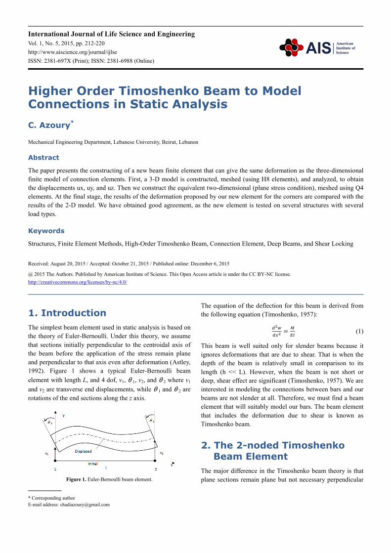
1992). Figure 1 shows a typical Euler-Bernoulli beam

element with length L, and 4 dof, v1, θ 1, v2, and θ 2 where v1

and v2 are transverse end displacements, while θ 1 and θ 2 are

rotations of the end sections along the z axis.

Figure 1. Euler-Bernoulli beam element.

The equation of the deflection for this beam is derived from

the following equation (Timoshenko, 1957):

������ �

��� (1)

This beam is well suited only for slender beams because it

ignores deformations that are due to shear. That is when the

depth of the beam is relatively small in comparison to its

length (h << L). However, when the beam is not short or

deep, shear effect are significant (Timoshenko, 1957). We are

interested in modeling the connections between bars and our

beams are not slender at all. Therefore, we must find a beam

element that will suitably model our bars. The beam element

that includes the deformation due to shear is known as

Timoshenko beam.

2. The 2-noded Timoshenko Beam Element

The major difference in the Timoshenko beam theory is that

plane sections remain plane but not necessary perpendicular

International Journal of Life Science and Engineering Vol. 1, No. 5, 2015, pp. 212-220 213

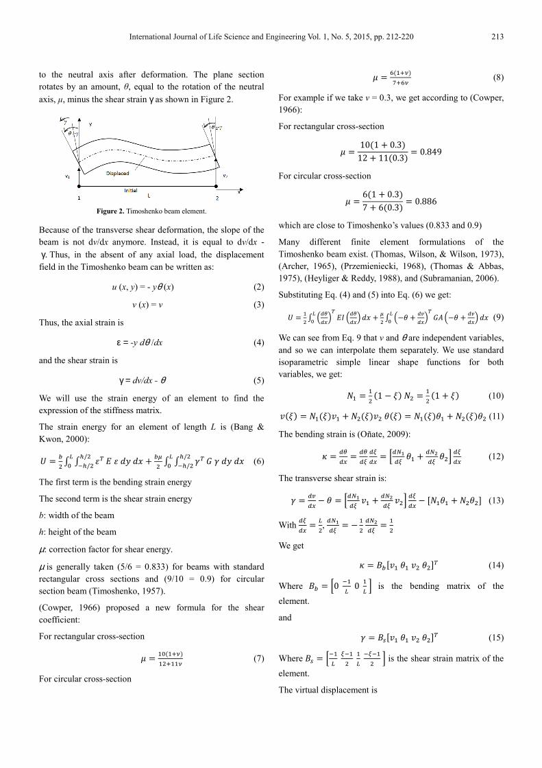
to the neutral axis after deformation. The plane section

rotates by an amount, θ, equal to the rotation of the neutral

axis, µ, minus the shear strain γ as shown in Figure 2.

Figure 2. Timoshenko beam element.

Because of the transverse shear deformation, the slope of the

beam is not dv/dx anymore. Instead, it is equal to dv/dx -

γ. Thus, in the absent of any axial load, the displacement

field in the Timoshenko beam can be written as:

u (x, y) = - yθ (x) (2)

v (x) = v (3)

Thus, the axial strain is

ε = -y dθ /dx (4)

and the shear strain is

γ = dv/dx - θ (5)

We will use the strain energy of an element to find the

expression of the stiffness matrix.

The strain energy for an element of length L is (Bang &

Kwon, 2000):

� � � � ��/�

��/��� � ���� � �

� � � ���/���/�

�� ������ (6)

The first term is the bending strain energy

The second term is the shear strain energy

b: width of the beam

h: height of the beam

µ: correction factor for shear energy.

µ is generally taken (5/6 = 0.833) for beams with standard

rectangular cross sections and (9/10 = 0.9) for circular

section beam (Timoshenko, 1957).

(Cowper, 1966) proposed a new formula for the shear

coefficient:

For rectangular cross-section

� � ���� !"�� ��! (7)

For circular cross-section

� � #�� !"$ #! (8)

For example if we take v = 0.3, we get according to (Cowper,

1966):

For rectangular cross-section

� � 10�1 � 0.3"12 � 11�0.3" � 0.849

For circular cross-section

� � 6�1 � 0.3"7 � 6�0.3" � 0.886

which are close to Timoshenko’s values (0.833 and 0.9)

Many different finite element formulations of the

Timoshenko beam exist. (Thomas, Wilson, & Wilson, 1973),

(Archer, 1965), (Przemieniecki, 1968), (Thomas & Abbas,

1975), (Heyliger & Reddy, 1988), and (Subramanian, 2006).

Substituting Eq. (4) and (5) into Eq. (6) we get:

� ��� /�0��1

��� �2 /�0��1�� �

�� � /34 � �5

��1��

� �6/34 � �5��1 �� (9)

We can see from Eq. 9 that v and θ are independent variables,

and so we can interpolate them separately. We use standard

isoparametric simple linear shape functions for both

variables, we get:

7� � �� �1 3 8"7� �

�� �1 � 8" (10)

9�8" � 7��8"9� � 7��8"9�4�8" � 7��8"4� � 7��8"4� (11)

The bending strain is (Oñate, 2009):

: � �0�� �

�0�;

�;�� � <

�=>�; 4� �

�=��; 4�?

�;�� (12)

The transverse shear strain is:

� � �5�� 3 4 � <

�=>�; 9� �

�=��; 9�?

�;�� 3 @7�4� � 7�4�A (13)

With �;�� �

��, �=>�; � 3

�� �=��; �

��

We get

: � B@9�4�9�4�A� (14)

Where B � <0 ��� 0��? is the bending matrix of the

element.

and

� � BC@9�4�9�4�A� (15)

Where BC � <��� ;���

�� �;��� ? is the shear strain matrix of the

element.

The virtual displacement is

214 C. Azoury: Higher Order Timoshenko Beam to Model Connections in Static Analysis

dv = N.@�9��4��9��4�A�

and the virtual strains are:

�: � B@�9��4��9��4�A�

�� � BC@�9��4��9��4�A�

The bending moment is M = Db.Bb.@9�4�9�4�A� where Db =

E I

And the shear force is V = Ds.Bs.@9�4�9�4�A� where Ds = µ

G A

We can show that bending stiffness matrix for the element is:

D � E B�FB��G

And the stiffness matrix element is:

DC � E BC�FCBC��G

And the equivalent nodal force vector is:

H � E 7. I��G

In the natural coordinate system,

D � E B�FB J2�8�

��DC � E BC�FCBC J2�8

�

��H � E 7. I J2�8

�

��

One thing to note here is that Kb is obtained using the exact

integration whereas Ks is obtained using the reduced

integration technique (one order less than required). This is to

avoid what is called shear locking. As the beam becomes

more slender, the bending strain energy becomes more

significant than the shear energy.

Upon integrating, we get:

Kb =

0 0 0 0

0 EI/L 0 -EI/L

0 0 0 0

0 -EI/L 0 EI/L

Ks =

µGA/L µGA/2 -µGA/L µGA/2

µGA/2 µGAL/4 -µGA/2 µGAL/4

-µGA/L -µGA/2 µGA/L -µGA/2

µGA/2 µGAL/4 -µGA/2 µGAL/4

f =

qL/2

0

qL/2

0

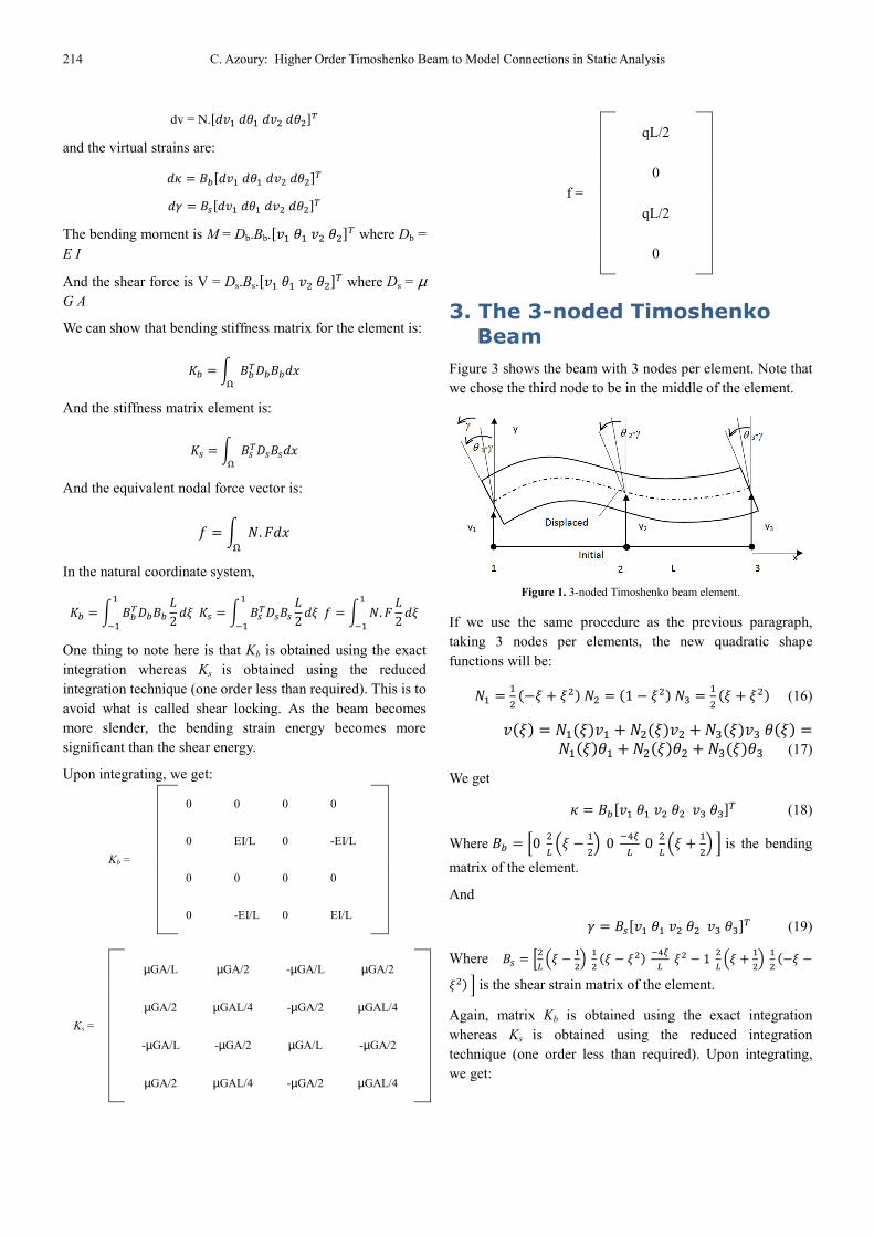
3. The 3-noded Timoshenko Beam

Figure 3 shows the beam with 3 nodes per element. Note that

we chose the third node to be in the middle of the element.

Figure 1. 3-noded Timoshenko beam element.

If we use the same procedure as the previous paragraph,

taking 3 nodes per elements, the new quadratic shape

functions will be:

7� � �� �38 � 8�"7� � �1 3 8�"7K �

�� �8 � 8�" (16)

9�8" � 7��8"9� �7��8"9� �7K�8"9K4�8" �7��8"4� �7��8"4� �7K�8"4K (17)

We get

: � B@9�4�9�4�9K4KA� (18)

Where B � <0 �� /8 3��1 0

�L;� 0 �� /8 �

��1? is the bending

matrix of the element.

And

� � BC@9�4�9�4�9K4KA� (19)

Where BC � <�� /8 3��1

�� �8 3 8�"

�L;� 8� 3 1

�� /8 �

��1

�� �38 3

8�"? is the shear strain matrix of the element.

Again, matrix Kb is obtained using the exact integration

whereas Ks is obtained using the reduced integration

technique (one order less than required). Upon integrating,

we get:

International Journal of Life Science and Engineering Vol. 1, No. 5, 2015, pp. 212-220 215

Kb =

0 0 0 0 0 0

0 7 0 -8 0 1

0 0 0 0 0 0

0 -8 0 16 0 -8

0 0 0 0 0 0

0 1 0 -8 0 7

Kb =µGA/(36L)

84 18L -96 24L 12 -6L

18L 4L2 -24L 4L

2 6L -2L

2

-96 -24L 192 0 -96 24L

24L 4L2 0 16 L

2 -24L 4L

2

12 6L -96 -24L 84 -18L

-6L -2L2 24L 4L

2 -18L 4L

2

f =

qL/6

0

2qL/3

0

qL/6

0

4. Testing the 3-noded Timoshenko Beam

Let test the new 3-noded Timoshenko beam on a cantilever

with a vertical force P on its tip.

Figure 2. Cantilever beam with tip end force.

The displacement from the thin beam theory is:

PL3/3EI

From the thick beam theory:

PL3/3EI + PLh

2/(10GI)

If we use just one element (3-noded Timoshenko) beam, it

will give the exact solution.

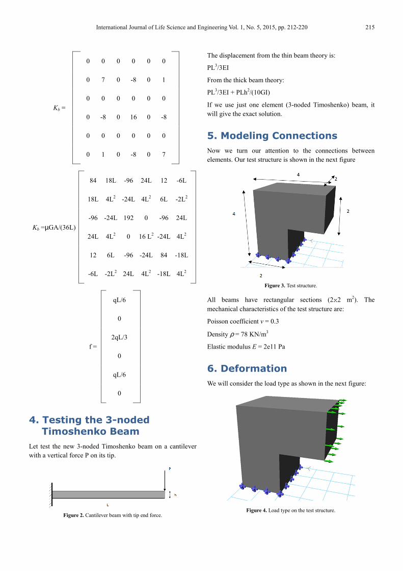
5. Modeling Connections

Now we turn our attention to the connections between

elements. Our test structure is shown in the next figure

Figure 3. Test structure.

All beams have rectangular sections (2x2 m2). The

mechanical characteristics of the test structure are:

Poisson coefficient v = 0.3

Density ρ = 78 KN/m3

Elastic modulus E = 2e11 Pa

6. Deformation

We will consider the load type as shown in the next figure:

Figure 4. Load type on the test structure.

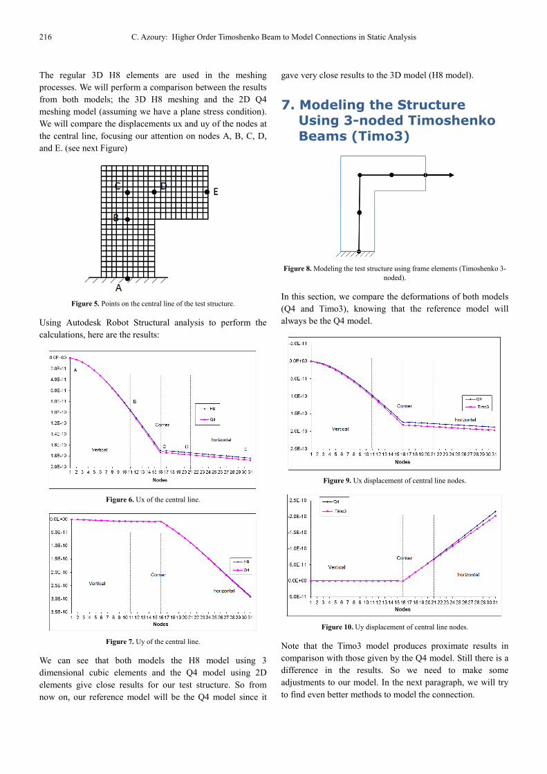
216 C. Azoury: Higher Order Timoshenko Beam to Model Connections in Static Analysis

The regular 3D H8 elements are used in the meshing

processes. We will perform a comparison between the results

from both models; the 3D H8 meshing and the 2D Q4

meshing model (assuming we have a plane stress condition).

We will compare the displacements ux and uy of the nodes at

the central line, focusing our attention on nodes A, B, C, D,

and E. (see next Figure)

Figure 5. Points on the central line of the test structure.

Using Autodesk Robot Structural analysis to perform the

calculations, here are the results:

Figure 6. Ux of the central line.

Figure 7. Uy of the central line.

We can see that both models the H8 model using 3

dimensional cubic elements and the Q4 model using 2D

elements give close results for our test structure. So from

now on, our reference model will be the Q4 model since it

gave very close results to the 3D model (H8 model).

7. Modeling the Structure Using 3-noded Timoshenko

Beams (Timo3)

Figure 8. Modeling the test structure using frame elements (Timoshenko 3-

noded).

In this section, we compare the deformations of both models

(Q4 and Timo3), knowing that the reference model will

always be the Q4 model.

Figure 9. Ux displacement of central line nodes.

Figure 10. Uy displacement of central line nodes.

Note that the Timo3 model produces proximate results in

comparison with those given by the Q4 model. Still there is a

difference in the results. So we need to make some

adjustments to our model. In the next paragraph, we will try

to find even better methods to model the connection.

International Journal of Life Science and Engineering Vol. 1, No. 5, 2015, pp. 212-220 217

8. Improved Model for the Connection

Our new element that will model the deformation of the

corner will be based on the utilization of Q4 surface

elements. We will use Timo3 elements to model non-corner

elements. One way to connect two different meshing types is

explained by (Dohrmann, Heinstein, & Key, 2000), (Zu-Qing

& Wenjun, 2000), and (Kattner & Crisinel, 2000).

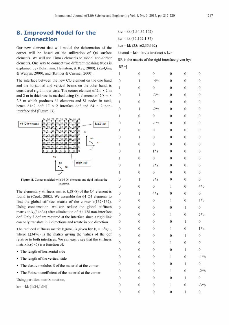
The interface between the new CQ element on the one hand

and the horizontal and vertical beams on the other hand, is

considered rigid in our case. The corner element of 2m × 2 m

and 2 m in thickness is meshed using Q4 elements of 2/8 m ×

2/8 m which produces 64 elements and 81 nodes in total,

hence 81×2 dof: 17 × 2 interface dof and 64 × 2 non-

interface dof (Figure 13).

Figure 11. Corner modeled with 64 Q4 elements and rigid links at the

intersect.

The elementary stiffness matrix ke(8×8) of the Q4 element is

found in (Cook, 2002). We assemble the 64 Q4 elements to

find the global stiffness matrix of the corner k(162×162).

Using condensation, we can reduce the global stiffness

matrix to kc(34×34) after elimination of the 128 non-interface

dof. Only 3 dof are required at the interface since a rigid link

can only translate in 2 directions and rotate in one direction.

The reduced stiffness matrix kr(6×6) is given by: kr = LTkcL,

where L(34×6) is the matrix giving the values of the dof

relative to both interfaces. We can easily see that the stiffness

matrix kr(6×6) is a function of:

� The length of horizontal side

� The length of the vertical side

� The elastic modulus E of the material at the corner

� The Poisson coefficient of the material at the corner

Using partition matrix notation,

krr = kk (1:34,1:34)

krc = kk (1:34,35:162)

kcr = kk (35:162,1:34)

kcc = kk (35:162,35:162)

kkcond = krr – krc x inv(kcc) x kcr

RR is the matrix of the rigid interface given by:

RR=[

1 0 0 0 0 0

0 1 -4*a 0 0 0

1 0 0 0 0 0

0 1 -3*a 0 0 0

1 0 0 0 0 0

0 1 -2*a 0 0 0

1 0 0 0 0 0

0 1 -1*a 0 0 0

1 0 0 0 0 0

0 1 0 0 0 0

1 0 0 0 0 0

0 1 1*a 0 0 0

1 0 0 0 0 0

0 1 2*a 0 0 0

1 0 0 0 0 0

0 1 3*a 0 0 0

0 0 0 1 0 4*b

0 1 4*a 0 0 0

0 0 0 1 0 3*b

0 0 0 0 1 0

0 0 0 1 0 2*b

0 0 0 0 1 0

0 0 0 1 0 1*b

0 0 0 0 1 0

0 0 0 1 0 0

0 0 0 0 1 0

0 0 0 1 0 -1*b

0 0 0 0 1 0

0 0 0 1 0 -2*b

0 0 0 0 1 0

0 0 0 1 0 -3*b

0 0 0 0 1 0

218 C. Azoury: Higher Order Timoshenko Beam to Model Connections in Static Analysis

0 0 0 1 0 -4*b

0 0 0 0 1 0

];

Where a and b are the width and column of the corner

divided by 8 respectively.

k(6×6) was found using Matlab® coding.

k = RR’ x kkcond x RR;

For our example of the test structure, the matrix k for the

corner is

5.0708e+11 1.6119e+11 -5.9359e+10 -5.0708e+11 -

1.6119e+11 -2.8653e+11

1.6119e+11 5.0708e+11 2.8653e+11 -1.6119e+11 -

5.0708e+11 5.9359e+10

-5.9359e+10 2.8653e+11 4.062e+11 5.9359e+10 -

2.8653e+11 -6.0307e+10

-5.0708e+11 -1.6119e+11 5.9359e+10 5.0708e+11

1.6119e+11 2.8653e+11

-1.6119e+11 -5.0708e+11 -2.8653e+11 1.6119e+11

5.0708e+11 -5.9359e+10

-2.8653e+11 5.9359e+10 -6.0307e+10 2.8653e+11 -

5.9359e+10 4.062e+11

Now that we have found the stiffness matrix of the corner

element and the stifnesss matrix of the Timo3 element, we

can model our frames with Timo3 elements and our corner

with a “64Q4condensed” element.

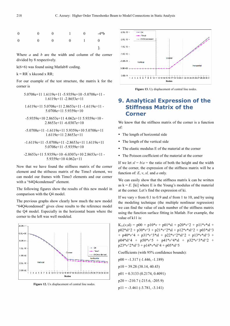
The following figures show the results of this new model in

comparison with the Q4 model.

The previous graphs show clearly how much the new model

“64Q4condensed” gives close results to the reference model

the Q4 model. Especially in the horizontal beam where the

corner to the left was well modeled.

Figure 12. Ux displacement of central line nodes.

Figure 13. Uy displacement of central line nodes.

9. Analytical Expression of the

Stiffness Matrix of the Corner

We know that the stiffness matrix of the corner is a function

of:

� The length of horizontal side

� The length of the vertical side

� The elastic modulus E of the material at the corner

� The Poisson coefficient of the material at the corner

If we let sl = b/a = the ratio of both the height and the width

of the corner, the expression of the stiffness matrix will be a

function of: E, v, sl, and a only.

We can easily show that the stiffness matrix k can be written

as k = E. [ki] where E is the Young’s modulus of the material

at the corner. Let’s find the expression of ki.

If we vary v from 0.1 to 0.9 and sl from 1 to 10, and by using

the modeling technique (the multiple nonlinear regression)

we can find the value of each number of the stiffness matrix

using the function surface fitting in Matlab. For example, the

value of k11 is:

K11(v,sl) = p00 + p10*v + p01*sl + p20*v^2 + p11*v*sl +

p02*sl^2 + p30*v^3 + p21*v^2*sl + p12*v*sl^2 + p03*sl^3

+ p40*v^4 + p31*v^3*sl + p22*v^2*sl^2 + p13*v*sl^3 +

p04*sl^4 + p50*v^5 + p41*v^4*sl + p32*v^3*sl^2 +

p23*v^2*sl^3 + p14*v*sl^4 + p05*sl^5

Coefficients (with 95% confidence bounds):

p00 = -1.317 (-1.446, -1.189)

p10 = 39.28 (38.14, 40.43)

p01 = 0.3133 (0.2174, 0.4091)

p20 = -210.7 (-215.6, -205.9)

p11 = -3.461 (-3.781, -3.141)

International Journal of Life Science and Engineering Vol. 1, No. 5, 2015, pp. 212-220 219

p02 = 0.03668 (0.0006138, 0.07274)

p30 = 496.4 (486.3, 506.5)

p21 = 15.54 (14.89, 16.19)

p12 = 0.01262 (-0.04434, 0.06957)

p03 = -0.00452 (-0.01133, 0.002292)

p40 = -529.8 (-540, -519.6)

p31 = -26.81 (-27.5, -26.12)

p22 = -0.01135 (-0.06805, 0.04535)

p13 = -0.00116 (-0.00655, 0.00423)

p04 = 0.0003249 (-0.0003018, 0.0009516)

p50 = 209.7 (205.7, 213.7)

p41 = 16.33 (16.02, 16.64)

p32 = 0.05683 (0.02995, 0.08371)

p23 = -0.003156 (-0.005549, -0.0007637)

p14 = 0.0001451 (-7.33e-05, 0.0003634)

p05 = -1.079e-05 (-3.316e-05, 1.157e-05)

Goodness of fit:

SSE: 39.05

R-square: 0.9986

Adjusted R-square: 0.9986

RMSE: 0.07289

and

k12(v,sl) = p00 + p10*v + p01*sl + p20*v^2 + p11*v*sl +

p02*sl^2 + p30*v^3 + p21*v^2*sl + p12*v*sl^2 + p03*sl^3

+ p40*v^4 + p31*v^3*sl + p22*v^2*sl^2 + p13*v*sl^3 +

p04*sl^4 + p50*v^5 + p41*v^4*sl + p32*v^3*sl^2 +

p23*v^2*sl^3 + p14*v*sl^4 + p05*sl^5

Coefficients (with 95% confidence bounds):

p00 = 0.1485 (0.1343, 0.1626)

p10 = 4.201 (4.075, 4.327)

p01 = -0.1236 (-0.1342, -0.1131)

p20 = -22.48 (-23.01, -21.95)

p11 = -0.002281 (-0.03751, 0.03295)

p02 = 0.02936 (0.02539, 0.03333)

p30 = 59.19 (58.09, 60.3)

p21 = 0.4262 (0.3547, 0.4977)

p12 = -0.02749 (-0.03376, -0.02123)

p03 = -0.003547 (-0.004296, -0.002797)

p40 = -70.68 (-71.8, -69.55)

p31 = -0.9373 (-1.013, -0.8614)

p22 = 0.01964 (0.01339, 0.02588)

p13 = 0.002219 (0.001626, 0.002812)

p04 = 0.0002156 (0.0001466, 0.0002845)

p50 = 32.05 (31.61, 32.49)

p41 = 0.6378 (0.6037, 0.6719)

p32 = -0.008022 (-0.01098, -0.005063)

p23 = -0.0005993 (-0.0008627, -0.000336)

p14 = -6.431e-05 (-8.834e-05, -4.027e-05)

p05 = -5.19e-06 (-7.651e-06, -2.728e-06)

Goodness of fit:

SSE: 0.4731

R-square: 0.9993

Adjusted R-square: 0.9993

RMSE: 0.008023

As we can see that, the R-square value for all the regression

analyses of all terms kij of the stiffness matrix are 0.99 and

that is a great correlation. Using this surface fitting in Matlab,

we could determine the coefficients of the condensed

stiffness matrix k for the connection.

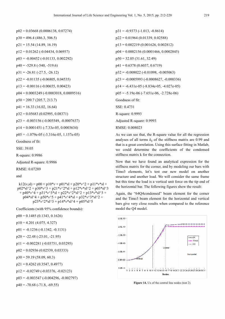
Now that we have found an analytical expression for the

stiffness matrix for the corner, and by modeling our bars with

Timo3 elements, let’s test our new model on another

structure and another load. We will consider the same frame

but this time the load is a vertical unit force on the tip end of

the horizontal bar. The following figures show the result:

Again, the “64Q4condensed” beam element for the corner

and the Timo3 beam element for the horizontal and vertical

bars give very close results when compared to the reference

model the Q4 model.

Figure 14. Ux of the central line nodes (test 2).

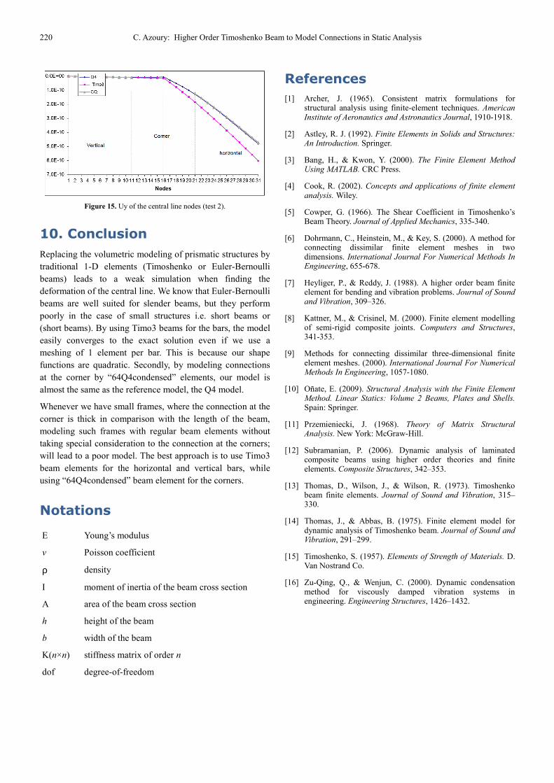
220 C. Azoury: Higher Order Timoshenko Beam to Model Connections in Static Analysis

Figure 15. Uy of the central line nodes (test 2).

10. Conclusion

Replacing the volumetric modeling of prismatic structures by

traditional 1-D elements (Timoshenko or Euler-Bernoulli

beams) leads to a weak simulation when finding the

deformation of the central line. We know that Euler-Bernoulli

beams are well suited for slender beams, but they perform

poorly in the case of small structures i.e. short beams or

(short beams). By using Timo3 beams for the bars, the model

easily converges to the exact solution even if we use a

meshing of 1 element per bar. This is because our shape

functions are quadratic. Secondly, by modeling connections

at the corner by “64Q4condensed” elements, our model is

almost the same as the reference model, the Q4 model.

Whenever we have small frames, where the connection at the

corner is thick in comparison with the length of the beam,

modeling such frames with regular beam elements without

taking special consideration to the connection at the corners;

will lead to a poor model. The best approach is to use Timo3

beam elements for the horizontal and vertical bars, while

using “64Q4condensed” beam element for the corners.

Notations

E Young’s modulus

v Poisson coefficient

ρ density

I moment of inertia of the beam cross section

A area of the beam cross section

h height of the beam

b width of the beam

K(n×n) stiffness matrix of order n

dof degree-of-freedom

References

[1] Archer, J. (1965). Consistent matrix formulations for structural analysis using finite-element techniques. American Institute of Aeronautics and Astronautics Journal, 1910-1918.

[2] Astley, R. J. (1992). Finite Elements in Solids and Structures: An Introduction. Springer.

[3] Bang, H., & Kwon, Y. (2000). The Finite Element Method Using MATLAB. CRC Press.

[4] Cook, R. (2002). Concepts and applications of finite element analysis. Wiley.

[5] Cowper, G. (1966). The Shear Coefficient in Timoshenko’s Beam Theory. Journal of Applied Mechanics, 335-340.

[6] Dohrmann, C., Heinstein, M., & Key, S. (2000). A method for connecting dissimilar finite element meshes in two dimensions. International Journal For Numerical Methods In Engineering, 655-678.

[7] Heyliger, P., & Reddy, J. (1988). A higher order beam finite element for bending and vibration problems. Journal of Sound and Vibration, 309–326.

[8] Kattner, M., & Crisinel, M. (2000). Finite element modelling of semi-rigid composite joints. Computers and Structures, 341-353.

[9] Methods for connecting dissimilar three-dimensional finite element meshes. (2000). International Journal For Numerical Methods In Engineering, 1057-1080.

[10] Oñate, E. (2009). Structural Analysis with the Finite Element Method. Linear Statics: Volume 2 Beams, Plates and Shells. Spain: Springer.

[11] Przemieniecki, J. (1968). Theory of Matrix Structural Analysis. New York: McGraw-Hill.

[12] Subramanian, P. (2006). Dynamic analysis of laminated composite beams using higher order theories and finite elements. Composite Structures, 342–353.

[13] Thomas, D., Wilson, J., & Wilson, R. (1973). Timoshenko beam finite elements. Journal of Sound and Vibration, 315–330.

[14] Thomas, J., & Abbas, B. (1975). Finite element model for dynamic analysis of Timoshenko beam. Journal of Sound and Vibration, 291–299.

[15] Timoshenko, S. (1957). Elements of Strength of Materials. D. Van Nostrand Co.

[16] Zu-Qing, Q., & Wenjun, C. (2000). Dynamic condensation method for viscously damped vibration systems in engineering. Engineering Structures, 1426–1432.