Boundary control of a rotating Timoshenko beam

ANZIAM J. 44 (E) ppE143–E184, 2003 E143

Boundary control of a rotatingTimoshenko beam

Stephen W. Taylor∗ Stephen C. B. Yau†

(Received 2 February 2002)

Abstract

The boundary control of a rotating beam is investigated.The beam is modelled by the Timoshenko beam equations,which are a system of two coupled wave equations that in-clude the effects of shearing and the rotational inertia ofcross-sections of the beam. The beam, which is pivoted atone end and free at the other, has physical parameters thatmay vary along the length of the beam. Conditions are foundfor which both the angle of rotation and the vibrations of thebeam may be controlled by applying a force at the free endand a torque at the pivoted end. This is an improvement onprevious work of the first author, who showed only that thevibrations may be controlled.

∗Department of Mathematics, University of Auckland, New Zealand.mailto:[email protected]

†Department of Mathematics, University of Auckland, New Zealand.mailto:[email protected]

0See http://anziamj.austms.org.au/V44/E033 for this article, c© Austral.Mathematical Soc. 2003. Published January 29, 2003. ISSN 1446-8735

mailto:[email protected]

mailto:[email protected]

http://anziamj.austms.org.au/V44/E033

Contents E144

Contents

1 Introduction E144

2 Timoshenko Beam Theory E1472.1 Basic Beam Theory . . . . . . . . . . . . . . . . . E1472.2 Characteristics of the beam . . . . . . . . . . . . E1502.3 Propagation of singularities . . . . . . . . . . . . E1532.4 Ratio of Moduli and Wave Speeds . . . . . . . . . E1552.5 Boundary Conditions . . . . . . . . . . . . . . . . E1562.6 Boundary Controllability of the non-Rotating Beams E1582.7 Existence of Solutions to the Beam Equations . . E159

3 A Rotating Timoshenko Beam E1633.1 Relative Motion of the Rotating Beam . . . . . . E1633.2 Energy and Equations of a Rotating Beam . . . . E1663.3 Partial Boundary Controllability of the Rotating Beam E1703.4 Existence of Solutions to the Beam Equations . . E172

4 An Auxiliary Problem and Boundary Controllabil-ity E1734.1 Auxiliary Problem and Contraction Properties . . E1734.2 Controlling the Hinged Beam . . . . . . . . . . . E1784.3 Controlling the Rotating Beam . . . . . . . . . . E180

References E183

1 Introduction

Vibration has long been known for its capacity for disturbance, dis-comfort, damage and destruction. Since ancient times, mankind hastried to investigate ways to control this phenomenon. Thus, in the

1 Introduction E145

development of control theory for partial differential equations overthe last few decades, it is not surprising that fundamental elasticsystems such as beams have received a lot of attention. The familiarEuler–Bernoulli beam equation has been the subject of many inves-tigations. In its simplest form this models the beam’s transversevibrations by the equation

ρAWTT + EIWXXXX = 0 .

Here the X-axis coincides with the beam when it is at rest andW (X,T ) is the displacement of the beam at time T in a directionthat is perpendicular to the X-axis. The parameters appearing hereare the beam’s density as mass per unit volume ρ, Young’s modulusof elasticity E, cross-sectional area A, and moment of inertia I.

The Timoshenko beam theory has also received some attention.This theory is an improvement of the Euler–Bernoulli system inthat it also takes into account rotational inertia and the shearingdeformation that occurs within a beam as it vibrates. The modelinvolves two coupled wave equations

ρAWTT + (kAG(Ψ−WX))X = 0 ,

ρIΨTT − (EIΨX)X + kAG(Ψ−WX) = 0 .

Here W and Ψ are the transverse and angular displacements respec-tively. This model is described in detail in the next section.

One way to impose controls for partial differential equations(pdes) is through boundary conditions. The space–variable domainfor a beam of length L may be taken to be the interval [0, L] whichhas boundary points X = 0 and X = L . Various boundary condi-tions are possible. For instance, if the beam is hinged at the origin

1 Introduction E146

and free at its other end then the boundary conditions take the form

W (0, T ) = 0 ,

EI(0)ΨX(0, T ) = −τ(T ) ,

ΨX(L, T ) = 0 ,

kAG(L)(Ψ(L, T )−WX(L, T )) = −f(T ) .

Here τ is an external torque applied at the origin and f is a forceapplied at the free end. Such boundary conditions are describedin greater detail in the next section. Null boundary controllabilityconcerns finding functions f and τ that drive solutions of the pdeto its zero displacement rest state during a specified time interval.The functions f and τ are often called controls or control functions.In fact, for linear systems such as this, null-controllability impliesthat initial states can be driven to any specified state.

The Timoshenko system is hyperbolic and consequently distur-bances move with finite speed along the beam. Because of this it isimpossible to control the Timoshenko beam within an indefinitelysmall time interval. In fact there is a time T0 associated with thespeed of propagation of singularities (see the next section for a de-scription of this) such that the beam is not controllable during timeintervals [0, t] if t < T0 . It is interesting to note that boundarycontrollability of the Euler–Bernoulli beam equation is possible forarbitrarily small time intervals.

The boundary controllability of hinged–free and clamped–freeTimoshenko beams is investigated in [6]. The hinged–free case ismore closely related to the case of a rotating beam, so we brieflydiscuss its controllability here. Provided that the control time ischosen to be greater than T0 , it is shown in [6] that the system maybe driven to one of its rest states if and only if there are no nontrivialsolutions of an overdetermined eigenvalue problem consisting of the

2 Timoshenko Beam Theory E147

des

µ2ρW − (kAG(Ψ−WX))X = 0 ,

µ2ρIΨ + (EIΨX)X − kAG(Ψ−WX) = 0 ,

and the six homogeneous boundary conditions

W (0) = 0 , Ψ(0) = 0 , ΨX(0) = 0 ,

W (L) = 0 , WX(L)−Ψ(L) = 0 , ΨX(L) = 0 .

It is shown in [6] that nontrivial solutions of this system exist forcertain values of the elastic parameters.

One shortfall of the theory developed in [6] is the fact that thehinged–free system has many rest states Ψ(X) = θ0 , W (X) = θ0X .A further shortfall is that the hinged-free beam is a simplistic modelof a rotating beam that allows for only small angular displacements.

The two main aims of this paper are to overcome these two short-falls. In fact in Section 3 we develop a better model for a rotatingTimoshenko beam which allows for larger angular displacementsand in Section 4 we modify our method to obtain controllabilityfor the θ0 = 0 case as well. A further aim is to correlate existinginformation on the Timoshenko Theory.

2 Timoshenko Beam Theory

2.1 Basic Beam Theory

The Timoshenko theory (or thick beam theory) accounts for boththe effect of rotary inertia and shear deformation, which are ne-glected when applied to Euler-Bernoulli beam theory (or thin beam


theory). The transverse vibration of the beam depends on its geo-metrical and material properties as well as the external applied forceand torque. The geometrical properties refer mainly to its length L,size and shape of its cross-section such as its area A, moment of iner-tia I with respect to the central axis of bending, and Timoshenko’sshear coefficient k which is a modifying factor (k < 1) to accountfor the distribution of shearing stress such that effective shear areais equal to kA. The material properties refer to its density ρ in massper unit volume, Young’s modulus or modulus of elasticity E andshear modulus or modulus of rigidity G. We assume that ρ, E, G,k, A and I are all positive, C2 functions of the space variable.

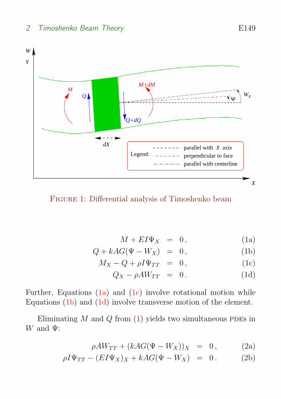
A differential element of a beam is shown in Figure 1. Here Wis the transverse displacement of the neutral line at a distance Xfrom the left end of the beam at time T . Due to the effect of shear,the original rectangular element changes its shape to somewhat likea parallelogram with its sides slightly curved.

The shear angle ϑ (or loss of slope) is now equal to the slope ofbending Ψ less slope of centerline WX in the form

ϑ = Ψ−WX ,

and the shear force Q is against the internal shear loading in theform

Q = −kAGϑ = −kAG(Ψ−WX) .

Similarly, the bending moment M is against the internal elasticinertia in the form

M = −EIΨX .

Moreover, from Figure 1, we equate the transverse force and rotaryinertia of the element to form the following four simultaneous pdes


M+dM

WXΨ

X

W

Y

Legend: parallel with X axisperpendicular to faceparallel with centerline

Q

dX

Q+dQ

M

Figure 1: Differential analysis of Timoshenko beam

M + EIΨX = 0 , (1a)

Q + kAG(Ψ−WX) = 0 , (1b)

MX −Q + ρIΨTT = 0 , (1c)

QX − ρAWTT = 0 . (1d)

Further, Equations (1a) and (1c) involve rotational motion whileEquations (1b) and (1d) involve transverse motion of the element.

Eliminating M and Q from (1) yields two simultaneous pdes inW and Ψ:

ρAWTT + (kAG(Ψ−WX))X = 0 , (2a)

ρIΨTT − (EIΨX)X + kAG(Ψ−WX) = 0 . (2b)


Equation (2a) is an equilibrium of translational force per unit lengthagainst the internal shear force gradient while Equation (2b) is anequilibrium of rotational torque per unit length equating to thegradient of internal bending moment against the internal shear force.This form is convenient for finding the normal modes and frequencyof free vibration and the solution is in the form of (W, Ψ) .

In the case of a uniform beam, Ψ can be eliminated from theabove two equations to form a single equation

EI

ρAWXXXX −

I

A

( E

kG+ 1)WXXTT +

ρI

kGAWTTTT + WTT = 0 . (3)

This equation has four terms in the unit of force per unit mass oracceleration. They are terms involving bending moment, shear force,rotational motion and translational motion respectively. When theshear and rotational terms are small and disregarded, the equationwill be that of the Euler-Bernoulli beam.

2.2 Characteristics of the beam

We differentiate (1a) and (1b) with respect to time T and introducenew variables, linear velocity V and angular velocity Ω to yield

ΩX +MT

EI= 0 , (4a)

VX −QT

kAG− Ω = 0 , (4b)

MX −Q + ρIΩT = 0 , (4c)

QX − ρAVT = 0 . (4d)

A linear combination of Equations (4a) and (4c) yields

α(MT + EIΩX) + MX + ρIΩT −Q = 0 , (5)


where α can be determined in such a way that the partial derivativesof the above equation combine to give total derivatives dM

dXand dΩ

dX

in the direction of unknown characteristic lines.

From dMdX

= MX + MTdTdX

, we have α = dTdX

and from dΩdX

=ΩX + ΩT

dTdX

, we have α = ρE

/dTdX

. Since the slope of characteristicsmust be the same in both cases

α2 =ρ

E

α =dT

dX= ±

√ρ

E= ± 1

v2

where v2 =√

E/ρ . Substituting these equations back into (5) andmultiplying by dT yields

± 1

v2

dM + ρIdΩ−QdT = 0 ,

where dT = ± 1v2

dX .

Similarly, a linear combination of Equations (4b) and (4d) yields

± 1

v1

dQ− ρAdV ± kAG

v1

ΩdT = 0

where v1 =√

kG/ρ and dT = ± 1v1

dX , hence the system of Equa-tions (4) is hyperbolic and associated with it are the four real char-acteristic equations:

I+ and I− ,dT

dX= ± 1

v2

; (6a)

II+ and II− ,dT

dX= ± 1

v1

. (6b)

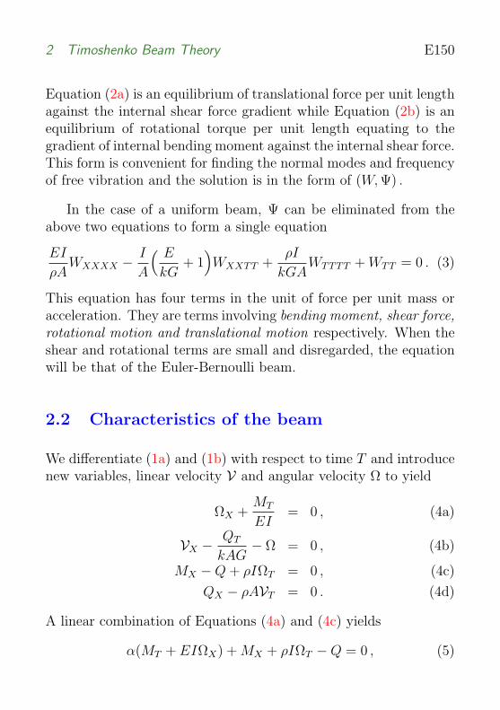
Figure 2 illustrates these four characteristics, I+, I− and II+, II−

passing through a point P in the space-time plane. By properties of


a

T

0X

I II II I

X X X X

− −

+ − −1 2 2 1+

+ +

P

b

Figure 2: The characteristics of Timoshenko equations throughpoint P


characteristics, the values of the unknowns M , Q, Ω and V at thepoint P depend only on their initial values on the X-axis, betweenX+

1 and X−1 for characteristics I+ and I−, and between X+

2 and X−2

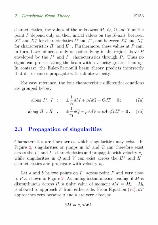
for characteristics II+ and II−. Furthermore, these values at P can,in turn, have influence only on points lying in the region above Penveloped by the I+ and I− characteristics through P . Thus nosignal can proceed along the beam with a velocity greater than v2 .In contrast, the Euler-Bernoulli beam theory predicts incorrectlythat disturbances propagate with infinite velocity.

For easy reference, the four characteristic differential equationsare grouped below:

along I+, I− : ± 1

v2

dM + ρIdΩ−QdT = 0 ; (7a)

along II+, II− : ± 1

v1

dQ− ρAdV ± ρAv1ΩdT = 0 . (7b)

2.3 Propagation of singularities

Characteristics are lines across which singularities may exist. InFigure 2, singularities or jumps in M and Ω can therefore existacross the I+ and I− characteristics and propagate with velocity v2,while singularities in Q and V can exist across the II+ and II−

characteristics and propagate with velocity v1.

Let a and b be two points on I− across point P and very closeto P as shown in Figure 2. Assuming instantaneous loading, if M isdiscontinuous across P , a finite value of moment δM = Ma − Mb

is allowed to approach P from either side. From Equation (7a), dTapproaches zero because a and b are very close, so

δM = v2ρIδΩ .


Thus, such jumps δM and δΩ across P will travel along character-istic I+ at speed v2. Similarly, the jumps on I+ across P will travelalong I− at speed v2 when passing through P . Applying the sametheory, similar results can be obtained with jumps δQ and δV for IIacross P with speed v1.

Taking account of the direction of the characteristics, we have:

along I+, I− : δM = ±v2ρIδΩ ; (8a)

along II+, II− : δQ = ∓v1ρAδV . (8b)

Hence a jump in M on I+ or I− is always accompanied by a definitejump in Ω. Similarly Q and V are coupled together.

From (7a) along I+, since Q is continuous across I+, the differ-ence across P gives

d(δM) + v2ρId(δΩ) = 0 ,

Eliminating δΩ from (8a),

d(δM) + v2ρId(δM

v2ρI) = 0 .

which can be integrated for a jump from point 1 to point 2 to give

(δM)2 = (δM)1

√(v2ρI)2

(v2ρI)1

.

Similarly, we eliminate δM from (8a) to give

(δΩ)2 = (δΩ)1

√(v2ρI)1

(v2ρI)2

.

It can be shown that the identical relationship holds between jumpsin M or 2 similar points on I− characteristics.


Applying the same theory to II yields

(δQ)2 = (δQ)1

√(v1ρA)2

(v1ρA)1

,

(δV)2 = (δV)1

√(v1ρA)1

(v1ρA)2

.

The interested reader may refer to John [2, p.35–37] or Leonard andBudiansky [3] for more details for propagation of singularities andtravelling waves in beams.

2.4 Ratio of Moduli and Wave Speeds

Hooke’s law states that the uniaxial stress σX (or axial force per unitsectional area) applied to a bar in the X direction is proportionalto the strain εX (or elongation per unit length) within the elasticlimit in the form

E =σX

εX

,

where the constant E is the modulus of elasticity. In the case of 3-dimensions, if a bar is lengthened by an axial force along the X-axis,there is always a corresponding reduction of length in the Y and Zdirections and a ratio known as Poisson’s ratio ν (0 < ν < 1) isintroduced. This ratio refers to the strains in these directions andis a constant for stresses within the elastic limit defined by

ν = − εY

εX

= − εZ

εX

(9)

where εX is the strain due only to the axial force in the X direction,and εY and εZ are the strains induced in the Y and Z directions


respectively. The minus sign indicates a decrease in transverse di-mensions when εX is positive, as in the case of tensile elongation.

G

E=

1

2(1 + ν).

Proof of this formula and further details can be obtained from mostMechanics or Strength of Material books such as [5] Pages 74–84.

Hence the ratio of wave speeds V can be derived directly fromk and ν as

V =v1

v2

=

√kG

E=

√k

2(1 + ν)<

1√2≈ 0.7071 . (10)

So in practice, G, E, v1 and v2 are all different such that 2G < Eand

√2v1 < v2 . Hence the characteristics are distinct.

Common values of Poisson’s ratio ν are 0.25 to 0.30 for steel,approximately 0.33 for most other metals, and 0.20 for concrete [5,p.43].

The Timoshenko shear coefficient k is derived by Mindlin andDeresiewics [4] to be π2/12 ≈ 0.822 for rectangular cross-sectionand 0.847 for circular cross-section.

2.5 Boundary Conditions

In general, there are three common types of boundary conditionsat each end of the beam. They are hinged, clamped and free type,again involving dynamics and geometrical properties of the beam:

hinged type W = 0 , M = EIΨX = 0 ;


clamped type W = 0 , Ψ = 0 ;

free type Q = kAG(Ψ−WX) = 0 , M = EIΨX = 0 .

The combination of the above at both ends of the beam yields six sit-uations: hinged-free, clamped-free, hinged-clamped, hinged-hinged,clamped-clamped, and free-free types.

In this section we investigate free vibration and controls mainlyon the hinged-free type (for convenience, hereafter we call it a hingedbeam). Also we study the clamped-free type (hereafter called aclamped beam), which has a similar set of equations to the hingedbeam, and use it for comparison of equations and as a test problemto test numerical code.

The control functions of the hinged beam with one end hinged atthe origin and the other end free, are a torque τ applied at the originand a force f applied at the free end. The associated boundaryconditions are

W (0, T ) = 0 , (11a)

EI(0)ΨX(0, T ) = −τ(T ) , (11b)

ΨX(L, T ) = 0 , (11c)

kAG(L)(Ψ(L, T )−WX(L, T )) = −f(T ) . (11d)

For the clamped beam with one end clamped at the origin and theother end free, the control functions are a force f and a torque τapplied at the free end. The associated boundary conditions for thiscase are

W (0, T ) = 0 , (12a)

Ψ(0, T ) = 0 , (12b)

kAG(L)(Ψ(L, T )−WX(L, T )) = −f(T ) , (12c)

EI(L)ΨX(L, T ) = −τ(T ) . (12d)


In each case, the system is completed by including the initial con-ditions

W (X, 0) = W o(X) , WT (X, 0) = Vo(X) , (13a)

Ψ(X, 0) = Ψo(X) , ΨT (X, 0) = Ωo(X) . (13b)

2.6 Boundary Controllability of thenon-Rotating Beams

Let T1 and T2 denote the times required for the two types of wavesto travel along the whole length of the hinged beam

T1 =

∫ L

0

dX

v1(X), T2 =

∫ L

0

dX

v2(X), (14)

and To = 2 max(T1, T2), and suppose that T > To . We seek controlfunctions f and τ belonging to L2(0, T ) for the hinged beam thatdrives the solutions to one of the states

WT (X, T ) = ΨT (X, T ) = 0 , Ψ(X, T ) = θo , W (X, T ) = θoX , (15)

where θo is a constant that can be interpreted as the weighted aver-age angle of rotation of the beam about the point at X = 0 .

For the clamped beam, solutions are driven to the states

W (X, T ) = Ψ(X, T ) = WT (X, T ) = ΨT (X, T ) = 0 .

In [6] it is shown that there are certain over-determined eigenvalueproblems associated with the hinged beam and the clamped beam.We discuss these here and that of a rotating beam in Section 4. Thecontrollability of each of these two beam systems is linked to thenon-existence of an eigenfunction, and uncontrollability is linked


to the existence of such an eigenfunction. For this reason, we callsuch eigenvalue problems controllability eigenvalue problems. Here,each eigenvalue problem with eigenvalue parameter µ consists of theordinary differential equations

µ2ρW − (kAG(Ψ−WX))X = 0 , (16a)

µ2ρIΨ + (EIΨX)X − kAG(Ψ−WX) = 0 , (16b)

and six homogeneous boundary conditions. The boundary condi-tions associated with the eigenvalue problem for the hinged beamare

W (0) = 0 , Ψ(0) = 0 , ΨX(0) = 0 , (17a)

W (L) = 0 , WX(L)−Ψ(L) = 0 , ΨX(L) = 0 . (17b)

The boundary conditions associated with the eigenvalue problemfor the clamped beam are

W (0) = 0 , W (L) = 0 , WX(L) = 0 , (18a)

Ψ(0) = 0 , Ψ(L) = 0 , ΨX(L) = 0 . (18b)

The eigenvalue problem for the clamped beam has only trivial solu-tions (one need consider only the boundary conditions at X = L tosee this), so it is controllable.

2.7 Existence of Solutions to the BeamEquations

To outline the existence theory of each of the systems (2), (11),(13) and the systems (2), (12), (13), we use the classical method ofcharacteristics approach as used in Section 2.2. In this section, we


assume that ρ, E, G, k, A and I are all positive, C1 functions ofthe space variable.

The analysis is simplified by introducing the column vector U =[U1, U2, U3, U4]

T where

U1 = −(√

kAG(Ψ−WX) +√

ρA WT )/2 , (19a)

U2 = −(√

kAG(Ψ−WX)−√

ρA WT )/2 , (19b)

U3 = −(√

EI ΨX −√

ρI ΨT )/2 , (19c)

U4 = −(√

EI ΨX +√

ρI ΨT )/2 , (19d)

from which we see that

U2 + U1 = −√

kAG(Ψ−WX) ,

U2 − U1 =√

ρA WT ,

U4 + U3 = −√

EI ΨX ,

U4 − U3 = −√

ρI ΨT .

The reason for coupling U1 and U2 together is that they areequations involving translational motion. Similarly, U3 and U4 arecoupled together because they are equations involving rotationalmotion.

The beam equations (2) are thus transformed to a single vectorequation

UT + ΛUX = BU− ΛXU/2, (20)

with

Λ =

v1

−v1

v2

−v2

and B =

0 b1 b2 −b2

−b1 0 b2 −b2

−b2 −b2 0 b3

b2 b2 −b3 0

,


where Λ is a diagonal matrix, v1 and v2 are speeds of the charac-teristics derived in Section 2.2, and B is a skew-symmetric matrixwith

b1 =1

2

(√

kAG

(1√ρA

)X

− (√

kAG )X√ρA

),

b2 = −1

2

√kAG

ρI,

b3 =1

2

(√

EI

(1√ρI

)X

− (√

EI )X√ρI

).

The mechanical energy of the beam is

E =1

2

∫ L

0

kAG(Ψ−WX)2 + ρAW 2T + EIΨ2

X + ρIΨ2T dX . (21)

In the new variables, the energy equation (21) is now in the form

E =

∫ L

0

U21 + U2

2 + U23 + U2

4 dX . (22)

Boundary conditions (11) for the hinged beam now take the form

U2(0, T )− U1(0, T ) = 0 , (23a)

U4(0, T ) + U3(0, T ) = (EI)(0)−1/2τ(T ) , (23b)

U4(L, T ) + U3(L, T ) = 0 , (23c)

U2(L, T ) + U1(L, T ) = (kAG)(L)−1/2f(T ) . (23d)

Boundary conditions (12) for the clamped beam take the form

U2(0, T )− U1(0, T ) = 0 , (24a)

U4(0, T )− U3(0, T ) = 0 , (24b)

U2(L, T ) + U1(L, T ) = (kAG)(L)−1/2f(T ) , (24c)

U4(L, T ) + U3(L, T ) = (EI)(L)−1/2τ(T ) . (24d)


In each case, the initial condition of the system can be denoted

U(X, 0) = g(X) . (25)

We quote herewith the theorems of Classical and Finite EnergySolutions without proof from the paper [6].

Theorem 1 (Classical Solutions) If the boundary data f , τ andthe initial data g are continuously differentiable and satisfy the ap-propriate compatibility conditions, then each of the systems (20),(23), (25) and that of (20), (24), (25) has a unique classical solu-tion.

Theorem 2 (Finite Energy Solutions I) If the boundary data f ,τ are in L2(0, T ) and the initial data g ∈ H , then each of the sys-tems (20), (23), (25) and that of (20), (24), (25) has a unique finiteenergy solution U . In fact, U ∈ C(0, T ;H) .

Theorem 3 (Finite Energy Solutions II) If the boundary data f ,τ are in L2(0, T ) and (W o, Ψo) ∈ Vh and (Vo, Ωo) ∈ Ho , then thesystem (2), (11), (25) has a unique weak solution (W, Ψ) such that(W, Ψ) ∈ C(0, T ;Vh) , (WT , ΨT ) ∈ C(0, T ;Ho) .

Here we define the finite energy space H = (L2(0, L))4 , the norm ofwhich is given by

‖U‖ =(∫ L

0

|U1|2 + |U2|2 + |U3|2 + |U4|2 dX)1/2

and say that a weak solution U is a finite energy solution if U ∈L∞(0, T ;H) . Also we set Ho = (L2(0, L))2 and Vh = (W, Ψ) ∈H1(0, L)2 : W (0) = 0 . Further we can state a theorem simi-lar to Theorem 3 for (2), (12), (25) by replacing Vh with Vc with

3 A Rotating Timoshenko Beam E163

Vc = (W, Ψ) ∈ H1(0, L)2 : W (0) = Ψ(0) = 0 where (W, Ψ) ∈C(0, T ;Vc) .

We again call such solutions finite energy solutions. The inter-ested reader may refer to paper [6] for proof. We will see that similarresults hold for the rotating beam.

3 A Rotating Timoshenko Beam

3.1 Relative Motion of the Rotating Beam

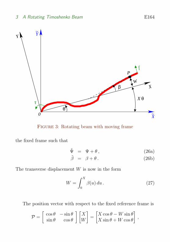
Consider a beam rotating anticlockwise about the pinned point atthe origin with its moving frame as indicated by X-Y axes which isinclined at an angle θ relative to a fixed reference frame as indicatedby X-Y axes at time T . The centerline of the beam is more orless coincident with the X-axis. More precisely, θ is the weightedaverage angle of inclination through the origin to be defined byEquation (30) and shown in Figure 3. Here we assume that thespeed of rotation is small so that any longitudinal elongation andstress of the beam due to rotation are small and may be neglected.

Let P = [X, W ]T be the position vector of a point P on thecenterline of the beam at a distance X from the origin. The tangentvector ∂P

∂Xof the centerline at P is inclined at an angle β with the

X-axis.

To avoid confusion and for our easy reference, we use nota-tions W , Ψ (and β to be defined as below), and X-Y axes in themoving frame as we have defined before as in Figure 1 and intro-duce the corresponding new notations W , Ψ, β and X-Y axes in


0

X

θτ

Y~

Y

X~

X

θ

βW

fP

Figure 3: Rotating beam with moving frame

the fixed frame such that

Ψ = Ψ + θ , (26a)

β = β + θ . (26b)

The transverse displacement W is now in the form

W =

∫ X

0

β(u) du . (27)

The position vector with respect to the fixed reference frame is

P =

[cos θ − sin θsin θ cos θ

] [XW

]=

[X cos θ −W sin θX sin θ + W cos θ

],


hence the velocity vector PT is given by

PT = (XθT + WT )

[− sin θ

cos θ

]−WθT

[cos θsin θ

]≈ (XθT + WT )

[− sin θ

cos θ

],

and

|PT |2 ≈ (XθT + WT )2 = W 2T ,

where

W =

∫ X

0

β(u) du = W + Xθ . (28)

To define the angle θ we need to express the idea that a certainweighted average of the displacements is zero in the moving coor-dinate frame. We soon see that there are mathematical advantagesto do this by requiring∫ L

0

ρIΨ + ρAXW dX = 0 , (29)

or ∫ L

0

ρI(Ψ− θ) + ρAX

∫ X

0

(β(u)− θ) du dX = 0 ,

from which we define the weighted average angle θ as

θ =

∫ L

0ρIΨ + ρAXW dX∫ L

0ρI + ρAX2 dX

. (30)


3.2 Energy and Equations of a Rotating Beam

The kinetic energy of the beam is in the form

KE =1

2

∫ L

0

ρIΨ2T + ρAW 2

T dX

=1

2

∫ L

0

ρI(ΨT + θT )2 + ρA(WT + XθT )2 dX

=1

2

∫ L

0

ρIΨ2T + ρAW 2

T + ρ(I + AX2)θ2T dX .

The potential energy of the beam is now in the form

PE =1

2

∫ L

0

EIΨ2X + kAG(Ψ− WX)2 dX.

=1

2

∫ L

0

EIΨ2X + kAG(Ψ−WX)2 dX .

The virtual work functional subjected to constraint (29) is now inthe form

W =

∫ T

0

KE− PE− γ(T )

∫ L

0

ρIΨ + ρAXW dX dT

where γ(T ) is the Lagrange multiplier associated with the constraintat time T . We calculate the first variation δW in order to apply theprinciple of virtual work and find the equations of motion. Applying


integration by parts yields

δW =

∫ T

0

∫ L

0

ρIΨT δΨT + ρAWT δWT + ρ(I + AX2)θT δθT

− EIΨXδΨX − kAG(Ψ−WX)(δΨ− δWX)

− γ(T )(ρIδΨ + ρAXδW ) dX dT

=

∫ L

0

[ρIΨT δΨ + ρAWT δW + ρ(I + AX2)θT δθ

]T0

dX

−∫ T

0

[EIΨXδΨ− kAG(Ψ−WX)δW

]L0

dT

−∫ T

0

∫ L

0

(ρIΨTT − (EIΨX)X + kAG(Ψ−WX) + ρIγ(T )

)δΨ

−(ρAWTT + (kAG(Ψ−WX))X + ρAXγ(T )

)δW

− ρ(I + AX2)θTT δθ dX dT .

For free vibration, and from Hamilton’s principle for conservativesystems as stated by Geradin and Rixen [1], δW = 0 so the coeffi-cients of δW , δΨ and δθ must all be zero in the integrand and alsoat the end points.

Equating the coefficients of δW , δΨ and δθ yields

ρA(WTT + Xγ(T )) + (kAG(Ψ−WX))X = 0 , (31a)

ρI(ΨTT + γ(T ))− (EIΨX)X + kAG(Ψ−WX) = 0 , (31b)

θTT

∫ L

0

ρ(I + AX2) dX = 0 . (31c)

with homogeneous boundary conditions

ΨX(0, T ) = ΨX(L, T ) = W (0, T ) = Ψ(L, T )−WX(L, T ) = 0 .

Also from Equation (31c), since the moment of inertia at the ori-

gin∫ L

0ρ(I + AX2) dX > 0 , the angular acceleration part θTT of


the equation must vanish, which means that the beam rotates withconstant angular velocity θT under free vibration.

When a torque τ(T ) is applied at X = 0 and a force f(T ) isapplied at X = L, we must add the following term to the virtualwork:

δW+ =

∫ T

0

fδ(displacement)|X=L + τδ(angle)|X=0 dT

=

∫ T

0

f(Lδθ + δW (L, T )) + τ(δθ + δΨ(0, T )) dT

=

∫ T

0

(fL + τ)δθ + fδW (L, T ) + τδΨ(0, T ) dT .

Equating the coefficient of δθ = 0 of the equation δ(W +W+) = 0yields

θTT

∫ L

0

ρ(I + AX2) dX = f(T )L + τ(T ) . (32)

The associated boundary conditions are

W (0, T ) = 0 , (33a)

EI(0)ΨX(0, T ) = −τ(T ) , (33b)

ΨX(L, T ) = 0 , (33c)

kAG(L)(Ψ(L, T )−WX(L, T )) = −f(T ) . (33d)

Taking second derivatives of Equation (29) and substituting (31),


(32) and (33) yields

0 =d2

dT 2

∫ L

0

ρIΨ + ρAXW dX

=

∫ L

0

(EIΨX)X − kAG(Ψ−WX)−X(kAG(Ψ−WX))X

− ρ(I + AX2)γ(T ) dX

=[EIΨX −XkAG(Ψ−WX)

]L0− γ(T )

∫ L

0

ρ(I + AX2) dX

= τ + fL− γ(T )

∫ L

0

ρ(I + AX2) dX

= (θTT − γ(T ))

∫ L

0

ρ(I + AX2) dX .

Hence the Lagrange multiplier γ is identified as the angular accel-eration:

γ(T ) = θTT . (34)

Substituting (34) into (31) yields

ρAWTT + (kAG(Ψ− WX))X = 0 , (35a)

ρIΨTT − (EIΨX)X + kAG(Ψ− WX) = 0 . (35b)

where W = W +Xθ and Ψ = Ψ+θ as defined. Hence Equation (35)has been put in exactly the same form as that of (2) simply byreplacing W with the arc length (W + Xθ) and Ψ by (Ψ + θ) asshown in Figure 3.

The associated boundary conditions of the rotating beam interms of W and Ψ are

W (0, T ) = 0 , (36a)

EI(0)ΨX(0, T ) = −τ(T ) , (36b)

ΨX(L, T ) = 0 , (36c)

kAG(L)(Ψ(L, T )− WX(L, T )) = −f(T ) , (36d)


which are identical to those of the hinged beam as given by Equa-tions (11).

3.3 Partial Boundary Controllability of theRotating Beam

Recall from Section 2.6 that the hinged beam can be driven to oneof the states given by (15)

WT (X, T ) = ΨT (X, T ) = 0 , Ψ(X, T ) = θo, W (X, T ) = θoX,

where θo is a constant and T > 2 max(T1, T2) with T1 and T2 definedby Equations (14). Consequently the rotating beam can be drivento one of the states

WT (X, T ) = ΨT (X, T ) = 0 ,

Ψ(X, T ) = θf , W (X, T ) = θfX, (37)

with θf = θo + θT where θT is the weighted average angular dis-placement of the beam at time T .

The following conditions are relevant to our controllability re-sults:

1. ρ, A, I, k, G and E are all positive functions of the spacevariable X and all belong to C2([0, L]) .

2. T > 2 max(T1, T2) .

We summarise these partial controllability results as a theorem.

Theorem 4 (Controllability) Suppose that conditions 1–2 abovehold. Then the following statements are true.


1. Suppose that there are no nontrivial solutions of the eigen-value problem (16), (17). Given finite energy initial data ofthe hinged beam problem (2), (11) and (25), there exist con-trol functions f ∈ L2(0, T ) and τ ∈ L2(0, T ) , that drive thesystem to its rest state at time T :

W (X, T )− θoX = Ψ(X, T )− θo = 0 ,

WT (X, T ) = ΨT (X, T ) = 0 , 0 < X < L .

2. Suppose that there are no nontrivial solutions of the eigen-value problem (16), (17). Given finite energy initial data ofthe rotating beam problem (35), (36) and (25), there exist con-trol functions f ∈ L2(0, T ) and τ ∈ L2(0, T ) , that drive thesystem to its rest state at time T :

W (X, T )− θfX = Ψ(X, T )− θf = 0 ,

WT (X, T ) = ΨT (X, T ) = 0 , 0 < X < L .

with θf = θo + θT where θT is the weighted average angulardisplacement of the beam at time T .

3. If there exist nontrivial solutions of the eigenvalue problem (16)and (17), then both the hinged problem (2), (11) and (25), andthe rotating problem (35), (36) and (25), are not even approx-imately controllable.


3.4 Existence of Solutions to the BeamEquations

For the system (35) and (36), we use U = [U1, U2, U3, U4]T in the

same way as in Section 2.7 and from (19)

U1 = −(√

kAG(Ψ− WX) +√

ρA WT )/2 ,

U2 = −(√

kAG(Ψ− WX)−√

ρA WT )/2 ,

U3 = −(√

EI ΨX −√

ρI ΨT )/2 ,

U4 = −(√

EI ΨX +√

ρI ΨT )/2 ,

with Equation (20) now taking the form

UT + ΛUX = BU− ΛXU/2 .

The mechanical energy of the beam is in the same form as (21)and (22):

E =1

2

∫ L

0

kAG(Ψ− WX)2 + ρAW 2T + EIΨ2

X + ρIΨ2T dX

=

∫ L

0

U21 + U2

2 + U23 + U2

4 dX

The boundary conditions analogous to (23) now take the form

U2(0, T )− U1(0, T ) = 0 , (38a)

U4(0, T ) + U3(0, T ) = (EI)(0)−1/2τ(T ) , (38b)

U4(L, T ) + U3(L, T ) = 0 , (38c)

U2(L, T ) + U1(L, T ) = (kAG)(L)−1/2f(T ) . (38d)

Also the system is completed by including the initial condition whichis the same as (25)

U(X, 0) = g(X) (39)

4 An Auxiliary Problem and Boundary Controllability E173

with the variation of θ given by (32).

Theorems 1-3 in Section 2.7 for the hinged beam are also validfor the rotating beam.

4 An Auxiliary Problem and

Boundary Controllability

So far we have been able to make use of (partial) controllabilityresults in [6] already proven for the hinged beam. To make furtherprogress and show that the rotating beam is (completely) control-lable, we modify the procedure followed in [6], which makes use ofa certain auxiliary problem to prove controllability.

4.1 Auxiliary Problem and ContractionProperties

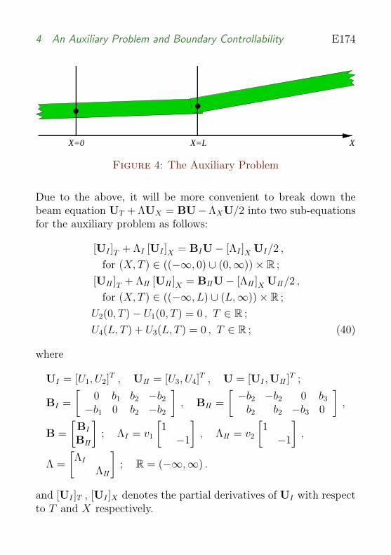
If the length of our hinged beam is extended from (0, L) to (−∞, L)and a second semi-infinite beam is hinged at the free end, we obtaina system which is very useful when considering controllability of theoriginal system. This system consists of two semi-infinite beams asshown in Figure 4 which represent what we call an auxiliary problem.The boundary conditions at X = 0 and X = L are

W (0, T ) = ΨX(L, T ) = 0 .

Further, since there is no external torque applied at the origin anddisplacement of the two beams must be the same at X = L, wehave

ΨX(0−, T ) = ΨX(0+, T ) , W (L−, T ) = W (L+, T ) .


X=0 X=L X

Figure 4: The Auxiliary Problem

Due to the above, it will be more convenient to break down thebeam equation UT + ΛUX = BU−ΛXU/2 into two sub-equationsfor the auxiliary problem as follows:

[UI ]T + ΛI [UI ]X = BIU− [ΛI ]X UI/2 ,

for (X, T ) ∈ ((−∞, 0) ∪ (0,∞))× R ;

[UII ]T + ΛII [UII ]X = BIIU− [ΛII ]X UII/2 ,

for (X, T ) ∈ ((−∞, L) ∪ (L,∞))× R ;

U2(0, T )− U1(0, T ) = 0 , T ∈ R ;

U4(L, T ) + U3(L, T ) = 0 , T ∈ R ; (40)

where

UI = [U1, U2]T , UII = [U3, U4]

T , U = [UI ,UII ]T ;

BI =

[0 b1 b2 −b2

−b1 0 b2 −b2

], BII =

[−b2 −b2 0 b3

b2 b2 −b3 0

],

B =

[BI

BII

]; ΛI = v1

[1−1

], ΛII = v2

[1−1

],

Λ =

[ΛI

ΛII

]; R = (−∞,∞) .

and [UI ]T , [UI ]X denotes the partial derivatives of UI with respectto T and X respectively.


For our controllability results we now assume that ρ, E, G, k,A and I are all positive, C2 functions of the space variable. Theproperties of the auxiliary problem that we need for proving con-trollability of the rotating beam have already been proven in [6].We summarise these below.

In the following theorems,

U(X, 0) = G(X) = [G1(X), G2(X), G3(X), G4(X)]T

and H = (L2(R))4 is the finite energy space with norm

‖U‖ =

(∫ ∞

−∞|U1|2 + |U2|2 + |U3|2 + |U4|2 dX

)1/2

,

and D is the set of functions U ∈ H such that

1. U1 and U2 are in H1(−∞, 0) and H1(0,∞) ,

2. U3 and U4 are in H1(−∞, L) and H1(L,∞) ,

3. U1−U2 and U3+U4 are almost everywhere equal to continuousfunctions, and in this sense U1(0)−U2(0) = 0 , U3(L)+U4(L) =0 .

For Theorem(5), we let B be the operator on H with domain Dgiven by

BU = −ΛUX − ΛXU/2 + BU . (41)

Theorem 5 (Finite Energy Solutions II) B is the infinitesimalgenerator of a strongly continuous unitary group U(T ) on H.


Of course, the fact that U(T ) is unitary for each T correspondsto conservation of energy for the physical system. The solution ofthe auxiliary problem with initial value g(X) is

U(X, T ) = U(T )g(X) .

Theorem 6 (Trace Property) The restrictions of components offinite energy solutions to lines parallel to the T -axis are locally L2 func-tions. Moreover, if U is such a solution, then the mapping X →Ui(X, ·) into L2

loc(R) , is continuous everywhere except possibly at X =0 for (40) and i = 1, 2, and at X = L for (40) and i = 3, 4. Atthese discontinuities, the left and right limits of the mapping exist.

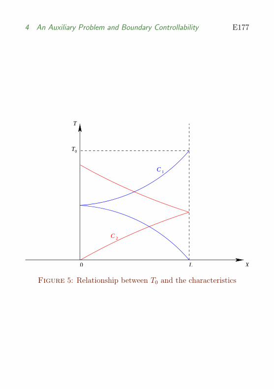
Recall that boundary control of hyperbolic systems requires atime interval determined by the speed of the characteristics. In ourcase we must take into account the time it takes for disturbancesto traverse the whole length [0, L] of the physical beam twice, asis illustrated in Figure 5. In this figure, C1 is the union of thecharacteristic with velocity −v1(X) starting at X = L, T = 0 andthe characteristic with velocity v1(X) starting at X = 0 at the timewhen the former characteristic meets the T -axis. C2 is a similarunion of characteristics with velocities ±v2(X) . We set

T0 = 2 max

(∫ L

0

ds

v1(s),

∫ L

0

ds

v2(s)

).

Let S be the subspace of H consisting of functions with supportsin the interval [0, L] and let P denote the projection onto S. ThusP may be regarded as the operator which multiplies functions bythe characteristic function of the interval [0, L].

Theorem 7 (Contraction Property) Suppose that


C

T

XL0

T0

C 1

2

Figure 5: Relationship between T0 and the characteristics


1. T > T0;

2. There are no non-trivial solutions of the over-determined eigen-value problem (16)–(17);

3. The wave speeds v1(X) and v2(X) are distinct at each pointX ∈ [0, L];

then ||PU(T )P|| < 1 .

The distinctness of the wave speeds is a technical requirement ofsome of the proofs in [6] and it is possible that it is not needed. How-ever, according to the discussion of Section 2.4, real beams satisfythis requirement anyway.

4.2 Controlling the Hinged Beam

Before considering the control of the rotating beam, it is instructiveto see how Theorem 4 for controllability of the hinged beam may bededuced from Theorem 7.

The idea is to start with initial data for the boundary controlproblem and extend it to be initial data for the auxiliary problemby letting it be equal to zero outside the interval [0, L]. Let g denotethe extension. Notice that g ∈ S . Next, we seek new initial dataf ∈ H such that:

1. f(X) = g(X) a.e. for X ∈ [0, L] ;

2. U(X, T ) = 0 a.e. for X ∈ [0, L] , where U(., T ) = U(T )f .


If we can find such initial data f then we can find appropriatecontrol functions f and τ for the boundary control problem by eval-uating the boundary conditions (38) for the known solution U(X, T )of the auxiliary problem. Further, the trace property, Theorem 6,shows that f, τ ∈ L2(0, T ) .

It remains to see how we can find f . The two conditions listedabove for f may be written

Pf = g , (42a)

PΦf = 0 , (42b)

where Φ = U(T ) . Φ is a unitary operator so Φ∗ = Φ−1 , whereΦ∗ and Φ−1 denote the dual and inverse of Φ respectively. Wenow see how to find such an f satisfying these properties and theadditional property that ||f || is the smallest possible.

We attempt to do this using Lagrange multipliers γ1 and γ2

belonging to H and the functional

J (f) =1

2(f , f)− (Pf − g, γ1)− (PΦf , γ2) .

The first variation of J is

δJ =1

2(f , δf) +

1

2(δf , f)− (Pδf , γ1)− (PΦδf , γ2)

= (δf , f)− (δf ,Pγ1)− (δf ,Φ∗Pγ2)

= (δf , f −Pγ1 −Φ∗Pγ2) .

The requirement that δJ = 0 yields

f = Pγ1 + Φ∗Pγ2. (43a)

Substituting (43a) into (42b) yields

PΦ(Pγ1 + Φ∗Pγ2) = 0 ,

Pγ2 = −PΦPγ1. (43b)


Substituting (43b) into (43a) yields

f = Pγ1 −Φ∗PΦPγ1 = (I−Φ∗PΦP)Pγ1, (43c)

where I denotes the 4× 4 identity matrix.

Substituting (43c) into (42a) yields

P(I−Φ∗PΦP)Pγ1 = g ,

Pγ1 = (I−PΦ∗PΦP)−1g . (43d)

Substituting (43d) into (43c) yields

f = (I−Φ∗PΦP)(I−PΦ∗PΦP)−1g . (44)

We suppose that the conditions of the contraction result, Theo-rem 7, are valid. If this is the case then ||PΦP|| < 1 and hence||PΦ∗PΦP|| < 1 , so the inverse operator appearing in Equation (44)is well defined and bounded. It is easy to verify that f satisfies therequired properties.

4.3 Controlling the Rotating Beam

The discussion above for the control of the hinged beam shows howthe beam may be brought to rest during a finite time interval but itdoes not address the final angle of inclination of the beam. In thissection we consider the additional constraint that the final angle ofinclination θ is zero.

Differentiating Equation (30) with respect to T yields

θT =

∫ L

0ρIΨT + ρAXWT dX∫ L

0ρ(I + AX2) dX

.


Integrating this over the time interval [0, T ] yields∫ T

0

∫ L

0

ρIΨT + ρAXWT dX dT = (θ(T )− θ(0))

∫ L

0

ρ(I + AX2) dX,

that is∫ T

0

∫ L

0

−√

ρI(U4 − U3) +√

ρA X(U2 − U1) dX dT = constant,

or ∫ T

0

(Z, U) dT = κ,

where Z(X) = [−√

ρA X,√

ρA X,√

ρI,−√

ρI ]T , U = [U1, U2, U3, U4]T

and (Z, U) denotes the Hilbert space inner product of Z and U. Theconstraint equation can be rewritten as∫ T

0

(Z, U) dT =

∫ T

0

(Z, PU(T )f) dT

=

(Z, P

∫ T

0

U(T ) dT f

)= (Z, PΩ(T ) f)

= κ .

where U(T ) = PU(T )f is equal to the solution in the interval [0, L]

and is zero outside the interval and Ω(T ) =∫ T

0U(T ) dT .

The constraint problem for rotating beam now takes the form:minimise

||f ||2 = (f , f) ,

subject to

Pf = g , (45a)

PΦf = 0 , (45b)

(PΩf ,Z) = κ . (45c)


Using Lagrange multipliers γ1 ∈ H , γ2 ∈ H and γ3 ∈ R , we have

J (f) =1

2(f , f)− (Pf − g, γ1)− (PΦf , γ2)− γ3((PΩf ,Z)− κ) ,

δJ = (δf , f)− (Pδf , γ1)− (PΦδf , γ2)− γ3(PΩδf ,Z)

= (δf , f −Pγ1 −Φ∗Pγ2)− γ3(δf ,Ω∗PZ)

= (δf , f −Pγ1 −Φ∗Pγ2 − γ3Ω∗PZ)

But we require δJ = 0 , so we have

f = Pγ1 + Φ∗Pγ2 + γ3Ω∗PZ . (46a)

Substituting (46a) into (45a) yields

Pγ1 + PΦ∗Pγ2 + γ3PΩ∗PZ = g . (46b)

Substituting (46a) into (45b) yields

Pγ2 = −(PΦPγ1 + γ3PΦΩ∗PZ) . (46c)

Substituting (46c) into (46b) yields

Pγ1 = −(I−PΦ∗PΦP)−1(γ3(P−PΦ∗PΦ)Ω∗PZ− g) . (46d)

Substituting (46c) and (46d) into (46a) yields

f = (I−Φ∗PΦP)Pγ1 + γ3(I−Φ∗PΦ)Ω∗PZ

= γ3(I−Φ∗PΦP− (I−PΦ∗PΦP)−1(P−PΦ∗PΦ))Ω∗PZ

+ (I−Φ∗PΦP)(I−PΦ∗PΦP)−1g

= γ3~a + ~b . (46e)

Substituting (46e) into (45c) yields

(PΩ(γ3~a + ~b),Z) = κ,

γ3(PΩ~a,Z) = κ− (PΩ~b,Z) ,

γ3 =κ− (PΩ~b,Z)

(PΩ~a,Z)(46f)

References E183

Finally, Substituting (46f) into (46e) yields

f =(κ− (PΩ~b,Z))

(PΩ~a,Z)~a + ~b , (47)

where the vectors

~a = (I−Φ∗PΦ− (I−PΦ∗PΦP)−1(P−PΦ∗PΦ))Ω∗PZ ,

~b = (I−Φ∗PΦP)(I−PΦ∗PΦP)−1g .

The control functions f and τ for the rotating beam are now foundas in the last section for the hinged beam. Note that we have oneextra condition for controllability: that (PΩ~a,Z) 6= 0 . Clearlythis condition, which may be verified for specific beams, must besatisfied for our method to work. However, it is not known if thecondition is necessary for boundary controllability.

References

[1] M. Geradin, D. Rixen, Mechanical Vibrations: Theory andApplication to Structural Dynamics, Wiley, Masson, (1994)E167

[2] F. John, Partial Differential Equations, Applied MathematicalSciences 1, Springer-Verlag, New York, 4th ed (1982). E155

[3] B. W. Leonard, B. Budiansky, On Travelling Waves in Beams,Natl. Adv. Comm. Aeron. Report 1173, 1-27 (1954) E155

[4] R. D. Mindlin, H. Deresiewics, Timoshenko’s ShearCoefficient for Flexural Vibrations of Beams, 2nd U.S. Natl.Cong. Appl. Mech., 175-178 (1955) E156

References E184

[5] A. Pytel, F. L. Singer, Strength of Materials Harper & Rows,New York 4th ed (1987) E156

[6] S. W. Taylor, A smoothing Property of a Hyperbolic Systemand Boundary Controllability, Journal of Computational andApplied Mathematics 114 23-40, N.H. Elsevier (2000) E146,E147, E158, E162, E163, E173, E175, E178

Documents

Boundary control of a rotating Timoshenko beam