Embed Size (px)
Citation preview
MODELING AND CONTROL OF THE TIMOSHENKO BEAM.THE DISTRIBUTED PORT HAMILTONIAN APPROACH∗
ALESSANDRO MACCHELLI† AND CLAUDIO MELCHIORRI†
SIAM J. CONTROL OPTIM. c© 2004 Society for Industrial and Applied MathematicsVol. 43, No. 2, pp. 743–767
Abstract. The purpose of this paper is to show how the Timoshenko beam can be fruitfullydescribed within the framework of distributed port Hamiltonian (dpH) systems so that rather simpleand elegant considerations can be drawn regarding both the modeling and control of this mechanicalsystem. After the dpH model of the beam is introduced, the control problem is discussed. Inparticular, it is shown how control approaches already presented in the literature can be unified,and a new control methodology is presented and discussed. This control methodology relies on thegeneralization to infinite dimensions of the concept of structural invariant (Casimir function) and onthe extension to distributed systems of the so-called control by interconnection methodology. In thisway, finite dimensional passive controllers can stabilize distributed parameter systems by shapingtheir total energy, i.e., by assigning a new minimum in the desired equilibrium configuration thatcan be reached if a dissipative effect is introduced.
Key words. modeling and control of flexible structures, Stokes–Dirac structures, infinite di-mensional port Hamiltonian systems, control by damping injection, Casimir functions, control byinterconnection
AMS subject classifications. 35Q72, 37K99, 93C20
DOI. 10.1137/S0363012903429530
1. Introduction. The port Hamiltonian approach has been introduced as a sys-tematic framework for geometric modeling and control of lumped-parameter physicalsystems [15, 26]. The port Hamiltonian model of a finite dimensional system takesits inspiration from circuit analysis: the behavior of a physical system is the result ofa network of atomic multiport elements, each of them characterized by a particularenergy property. The key point is the identification of the interconnection structure,mathematically described by a Dirac structure [2, 26], a generalization of the well-known Kirchhoff laws [16]. In this way, the variation of a system’s total energy isrelated to the power exchanged with the environment, and the dynamics is the resultof internal power flows among different parts of the whole system. It has been shownthat this approach can be fruitfully applied for modeling a wide class of physical (me-chanical, electrical, hydraulic, and chemical) systems, and several control techniques,based on energy considerations, have been developed in order to solve the regulationproblem [20, 21, 26].
In some sense, it seems natural to extend the finite dimensional Hamiltonianformulation in order to deal with distributed parameter systems. Many results onintegrability, existence of solutions or stability, and several applications have beenproposed in the last decades; see, for example, [24] for an application to fluid dynamicsand [19] for a nice introduction and historical remarks. On the other hand, it isinteresting to note that some problems regarding the treatment of boundary conditionsare still open. In fact, most of the research activity has been focused on the study of
∗Received by the editors June 9, 2003; accepted for publication (in revised form) December 18,2003; published electronically August 27, 2004. This research activity has been performed in thecontext of the European project GeoPlex, reference code IST-2001-34166. Further information isavailable at http://www.geoplex.cc.
http://www.siam.org/journals/sicon/43-2/42953.html†Department of Electronics, Computer Science and Systems (DEIS), University of Bologna, viale
Risorgimento 2, 40136 Bologna, Italy ([email protected], [email protected]).
743
744 ALESSANDRO MACCHELLI AND CLAUDIO MELCHIORRI
infinite dimensional systems characterized by an infinite spatial domain, for which thestate variables tend to zero when the spatial variable tends to infinity (with respectto some norm), or on the analysis of infinite dimensional systems with zero boundaryconditions (on the finite spatial domain).
These are autonomous systems: no interaction, i.e., power exchange, with theenvironment is taken into account. This is a strong limitation since it is not possibleto study the effect of nonzero boundary conditions (e.g., voltages and currents at bothends of a transmission line) on the dynamics of the system. In this way, it is difficultto deal with control application for infinite dimensional systems in Hamiltonian form.The controller, in fact, can act on the system only by properly modifying the boundaryvariables or, equivalently, by exchanging power with the (infinite dimensional) system.
From a mathematical point of view, it is not evident how a nonzero energy flowthrough the boundary can be incorporated into the classical distributed Hamiltonianframework. The key point is the notion of Dirac structure in infinite dimensions thatwill be defined, in this case, on a space of differential forms on the spatial domain ofthe system and its boundary. Since the relation between variation of internal energyand power flow through the boundary relies on the Stokes theorem [17, 18], thesestructures are called Stokes–Dirac structures.
Once the Stokes–Dirac structure of a particular infinite dimensional system isdeduced, the distributed port Hamiltonian (dpH) model follows automatically [17,18] and the control problem can be approached. When dealing with the control ofdistributed parameter systems, the main problem concerns the intrinsic difficultiesrelated to the proof of stability of an equilibrium configuration. It is important toemphasize that this limitation does not depend on the particular approach adopted.Even if a distributed parameter system is described within the port Hamiltonianframework, the stability proof of a certain control scheme will always be a difficulttask. On the other hand, the main advantages in adopting the dpH framework canbe the following:
• The development of control schemes for infinite dimensional systems is usu-ally based on energy considerations or, equivalently, the stability proof oftenrelies on the properties of an energy-like functional, a generalization of theLyapunov function to the distributed parameters case. The Hamiltonian de-scription of a distributed parameter system is given in terms of time evolutionof energy variables depending on the variation of the total energy of the sys-tem. In this way, the energy of the system, which is generally a good Lyapunovfunction, appears explicitly in the mathematical model of the system itselfand, consequently, both the design of the control law and the proof of itsstability can be deduced and presented in a more intuitive (in some sensephysical) and elegant way.
• The port Hamiltonian formulation of distributed parameter systems deeplyrelies on the notion of Dirac structure, as in finite dimensions. This fact isimportant and allows us to go further; in particular, it is of great interestto understand whether the control schemes developed for finite dimensionalport Hamiltonian systems could also be generalized in order to deal withthe distributed parameter case. For example, suppose that the total energy(Hamiltonian) of the system is characterized by a minimum at the desiredequilibrium configuration. This happens, for example, in the case of flexi-ble beams, for which the zero-energy configuration corresponds to the unde-formed beam. In this situation, the controller can be developed in order to
MODELING AND CONTROL OF THE TIMOSHENKO BEAM 745
behave as a dissipative element to be connected to the system at the bound-ary or along the distributed port. The amount of dissipated power can beincreased in order to quickly reach the configuration with minimum energy.As in the finite dimensional case, it can happen that the minimum of the en-ergy does not correspond to a desired configuration. Then it is necessary toshape the energy function so that a new minimum is introduced. This can beachieved by generalizing the control by interconnection and energy-shapingmethodology to deal with distributed parameter systems, as presented in [22],where the infinite dimensional system is a lossless transmission line.
In this paper, it is shown how the modeling and control problems of an infinitedimensional system, the Timoshenko beam, can be solved within the framework ofdpH systems. Flexible beams are generally modeled according to the classical Euler–Bernoulli theory: this formulation provides a good description of the dynamical be-havior of the system if the beam’s cross sectional dimension is small in comparison toits length. In this case, the effects of the rotary inertia of the beam are not consid-ered. A more accurate beam model is provided by the Timoshenko theory, accordingto which the rotary inertia and also the deformation due to shear are considered.The resulting Timoshenko model of the beam is generally more accurate in predictingthe beam’s response than the Euler–Bernoulli one but, on the other hand, it is moredifficult to utilize for control purposes because of its complexity.
As already pointed out, the dpH formulation of the Timoshenko model of thebeam [6] (but refer also to [7, 11, 12]) does not reduce the complexity of the modelitself, but it is useful both for modeling considerations and control purposes. From themodeling point of view, the internal and external interconnections of the system arerevealed: it is clear how the kinetic and potential elastic energy domains interact andhow the system can exchange power with the environment through its border and/or adistributed port. Furthermore, the dpH representation of the system makes it possibleto extend well-established passive control strategies that were originally developed forfinite dimensional port Hamiltonian systems and to elegantly unify control approachesalready presented in the literature [8, 25].
The paper is organized as follows. In section 2, a brief background on Diracstructures and on the classical formulation of the Timoshenko model of the beam isprovided, and then the Stokes–Dirac structure of the Timoshenko beam is presentedand the dpH model introduced. The control problem is approached in sections 3 and4. In section 3, the control by damping injection methodology is extended to infinitedimensions in order to stabilize the beam in its undeformed configuration, as alreadypresented in [8, 25]. In section 4, the control by interconnection and energy shapingmethodology [20, 26, 21] is extended to distributed parameter systems in order tocontrol a mechanical system made of a flexible (Timoshenko) beam with a rigid bodyconnected at one of its extremities. The finite dimensional controller, acting on thesystem through the other extremity, is developed by properly extending the conceptof Casimir functions to the infinite dimensional case and by generalizing the resultspresented in [22] (see also [12, 11]). Finally, conclusions and suggestions for futurework are illustrated in section 5.
2. Timoshenko beam in dpH form.
2.1. Timoshenko beam—the classical formulation. According to the Tim-oshenko theory, the motion of a beam can be described by the following system of

746 ALESSANDRO MACCHELLI AND CLAUDIO MELCHIORRI
PDEs:
ρ∂2w
∂t2−K
∂2w
∂x2+ K
∂φ
∂x= 0,
Iρ∂2φ
∂t2− EI
∂2φ
∂x2+ K
(φ− ∂w
∂x
)= 0,
(2.1)
where t is the time and x ∈ [0, L] is the spatial coordinate along the beam in itsequilibrium position, and w(x, t) is the deflection of the beam from the equilibriumconfiguration and φ(x, t) is the rotation of the beam’s cross section due to bending;the motion takes place in the wx-plane. Denote by D := [0, L] the spatial domain andby ∂D = 0, L its boundary.
The coefficients ρ, Iρ, E, and I, assumed to be constant, are the mass per unitlength, the mass moment of inertia of the cross section, Young’s modulus, and themoment of inertia of the cross section, respectively. The coefficient K is equal tokGA, where G is the modulus of elasticity in shear, A is the cross sectional area, andk is a constant depending on the shape of the cross section.
The mechanical energy is given by the following relation [8]:
H(t) :=
kinetic energy︷ ︸︸ ︷1
2
∫ L
0
ρ
(∂w
∂t
)2
+ Iρ
(∂φ
∂t
)2
dx
+1
2
∫ L
0
K
(φ− ∂w
∂x
)2
+ EI
(∂φ
∂x
)2
dx︸ ︷︷ ︸potential elastic energy
.
(2.2)
Note the presence of two interactive energy domains, the kinetic and the potentialelastic.
2.2. Dirac structures. The starting point in the definition of a port Hamilto-nian system (both finite and infinite dimensional) is the identification of a suitablespace of power variables, strictly related to the geometry of the system, and the defi-nition of a Dirac structure on this space of power variables, in order to describe theinternal and external interconnection of the system. The Dirac structures were intro-duced in [2], while in [4, 26] it is pointed out that they are the geometric tool thatallows us to formalize and generalize the notion of power-conserving interconnection.
Before stating the general definition of Dirac structure, it is necessary to introducethe space of power variables. Consider a linear space F , possibly infinite dimensional(space of generalized velocities or flows), and denote by E = F∗ its dual (space ofgeneralized forces or efforts). The space of power variables is F ×E . Then, from [18],we take the following fundamental definition.
Definition 2.1 (Dirac structure). Denote by F × E a space of power variables(possibly infinite dimensional). There exists on F × E the canonically defined sym-metric bilinear form (+pairing operator)
(f1, e1), (f2, e2) := 〈e1, f2〉 + 〈e2, f1〉 ,(2.3)
where fi ∈ F , ei ∈ E, i = 1, 2, and 〈·, ·〉 denotes the duality product between F and itsdual space E. A constant Dirac structure on F is a linear subspace D ⊂ F × E suchthat
D = D⊥,(2.4)

MODELING AND CONTROL OF THE TIMOSHENKO BEAM 747
where ⊥ denotes the orthogonal complement with respect to the bilinear form ·, · .An immediate consequence of the previous definition is that, if (f, e) ∈ D, then
0 = (f, e), (f, e) = 2 〈e, f〉 .(2.5)
Consequently, 〈e, f〉 = 0 for every (f, e) ∈ D. In other words, if (f, e) ∈ F × Eis a couple of power conjugated variables, the fact that they belong to the Diracstructure D implies power conservation, i.e., the dual product is equal to 0. The Diracstructure is the geometrical tool by means of which it is possible to deal with power-conserving interconnection in physical systems. As will be pointed out in section 2.4for the Timoshenko beam, once a proper interconnection structure is defined, the portHamiltonian model of a physical system follows automatically.
2.3. Timoshenko beam—The Stokes–Dirac structure. Consider the me-chanical energy (2.2). The potential elastic energy is a function of the shear and ofthe bending, given by the following 1-forms:
εt(t, x) =
[∂w
∂x(t, x) − φ(t, x)
]dx, εr(t, x) =
∂φ
∂x(t, x)dx.(2.6)
The associated coenergy variables are the 0-forms (functions) shear force and thebending momentum, given by σt(t, x) = K∗εt(t, x) and σr(t, x) = EI∗εr(t, x), where ∗is the Hodge star operator defined, for example, in [14]. Besides, the kinetic energy isa function of the translational and rotational momenta, i.e., of the following 1-form:
pt(t, x) = ρ∂w
∂t(t, x)dx, pr(t, x) = Iρ
∂φ
∂t(t, x)dx,(2.7)
and the associated coenergy variables are the 0-forms translational and rotationalmomenta, given by vt(t, x) = 1
ρ∗pt(t, x) and vr(t, x) = 1Iρ∗pr(t, x).
Consider an n-dimensional (Riemannian) manifold N and denote by Ωk(N ) thespace of k-forms on N , i.e., the space of k-linear alternating functions. So, we havethat pt, pr, εt, εr ∈ Ω1(D) and that w, φ ∈ Ω0(D). If d : Ωk(N ) → Ωk+1(N ) is theexterior derivative on the space of forms, it is possible to rewrite (2.6) and (2.7) as
pt = ρ∗∂w∂t
, εt = dw − ∗φ, pr = Iρ∗∂φ
∂t, εr = dφ,
and the total energy (2.2) becomes the following (quadratic) functional:
H(pt, pr, εt, εr) =
∫DH(pt, pr, εt, εr)
=1
2
∫D
(1
ρ∗pt ∧ pt +
1
Iρ∗pr ∧ pr + K∗εt ∧ εt + EI∗εr ∧ εr
)(2.8)
with H : Ω1(D) × · · · × Ω1(D) × D → Ω1(D) the energy density. Consider a timefunction
(pt(t), pr(t), εt(t), εr(t)) ∈ Ω1(D) × · · · × Ω1(D)
with t ∈ R, and evaluate the energy H along this trajectory. At any time t, thevariation of internal energy, that is, the power exchanged with the environment, is

748 ALESSANDRO MACCHELLI AND CLAUDIO MELCHIORRI
given by
dHdt
=
∫D
(δptH ∧ ∂pt
∂t+ δprH ∧ ∂pr
∂t+ δεtH ∧ ∂εt
∂t+ δεrH ∧ ∂εr
∂t
)
=
∫D
[(1
ρ∗pt)∧ ∂pt
∂t+
(1
Iρ∗pr)∧ ∂pr
∂t+ (K∗εt) ∧
∂εt∂t
+ (EI∗εr) ∧∂εr∂t
].
(2.9)
The differential forms ∂pt
∂t , ∂pr
∂t , ∂εt∂t , and ∂εr
∂t are the time derivatives of the energyvariables pt, pr, εt, and εr and represent the generalized velocities (flows), while δpt
H,δpr
H, δεtH, and δεrH are the variational derivatives of the total energy (2.8). Theyare related to the rate of change of the stored energy and represent the generalizedforces (efforts).
The dpH formulation of the Timoshenko beam can be obtained either by express-ing (2.1) in terms of pt, pr, εr, and εt as introduced in (2.6) and (2.7), or, in a morerigorous way, by revealing the underlying Dirac structure of the model. For this pur-pose, it is necessary to define the space of power variables. The space of flows is givenby
F := Ω1(D) × Ω1(D) × Ω1(D) × Ω1(D)︸ ︷︷ ︸generalized velocities
×Ω0(∂D) × Ω0(∂D)︸ ︷︷ ︸border flow
,(2.10)
and it is well known that the space of effort E is the dual of F . The concept of dualityover the space of forms can be given by the following proposition [17].
Proposition 2.2. Consider an n-dimensional Riemannian manifold N . Thenthe dual space (Ωk(N ))∗ of Ωk(N ) can be identified with Ωn−k(N ) and the dualityproduct between Ωk(N ) and (Ωk(N ))∗ by
〈β, α〉 :=
∫Nα ∧ β(2.11)
with α ∈ Ωk(N ) and β ∈ Ωn−k(N ). The same result holds for Ωk(∂N ).An immediate consequence of Proposition 2.2 is that the dual space E of F , the
space of efforts, can be easily identified with
E := Ω0(D) × Ω0(D) × Ω0(D) × Ω0(D)︸ ︷︷ ︸generalized forces
×Ω0(∂D) × Ω0(∂D)︸ ︷︷ ︸border effort
.(2.12)
Thus, the duality product (2.11) and the +pairing operator (2.3) can be easily spe-cialized in order to deal with the space of power variables F ×E defined by (2.10) and(2.12). Suppose that
(fpt , fpr , fεt , fεr , f
tb , f
rb , ept , epr , eεt , eεr , e
tb, e
rb
),(f ipt, . . . , fr,i
b , eipt, . . . , er,ib
)∈ F × E
MODELING AND CONTROL OF THE TIMOSHENKO BEAM 749
with i = 1, 2. Then
〈(ept , epr , eεt , eεr , etb, e
rb) , (fpt , fpr , fεt , fεr , f
tb , f
rb )〉
:=
∫D
(fpt∧ ept
+ fpr∧ epr
+ fεt ∧ eεt + fεr ∧ eεr ) +
∫∂D
(f tb ∧ etb + fr
b ∧ erb),
(f1pt, . . . , fr,1
b , e1pt, . . . , er,1b ,
)(f2pt, . . . , fr,2
b , e2pt, . . . , er,2b
)
:=
∫D
(f1pt
∧ e2pt
+ f2pt
∧ e1pt
+ f1pr
∧ e2pr
+ f2pr
∧ e1pr
)+
∫D
(f1εt ∧ e2
εt + f2εt ∧ e1
εt + f1εr ∧ e2
εr + f2εr ∧ e1
εr
)+
∫∂D
(f t,1b ∧ et,2b + f t,2
b ∧ et,1b + fr,1b ∧ er,2b + fr,2
b ∧ er,1b
).
(2.13)With the following proposition, the main result of this section is presented.
Proposition 2.3 (the Timoshenko beam Dirac structure). Consider the space ofpower variables F×E with F and E defined in (2.10) and (2.12) and the bilinear form(+pairing operator) ·, · given by (2.13). Define the following linear subspace D
of F × E:
D =
⎧⎪⎪⎨⎪⎪⎩ (fpt , fpr , fεt , fεr , f
tb , f
rb , ept , epr , eεt , eεr , e
tb, e
rb) ∈ F × E |
⎡⎢⎢⎣
fpt
fpr
fεtfεr
⎤⎥⎥⎦ = −
⎡⎢⎢⎣
0 0 d 00 0 ∗ dd −∗ 0 00 d 0 0
⎤⎥⎥⎦⎡⎢⎢⎣
ept
epr
eεteεr
⎤⎥⎥⎦ ,
⎡⎢⎢⎣
f tb
frb
etberb
⎤⎥⎥⎦ =
⎡⎢⎢⎣
ept|∂D
epr |∂Deεt |∂Deεr |∂D
⎤⎥⎥⎦⎫⎪⎪⎬⎪⎪⎭ ,
(2.14)where |∂D denotes the restriction on the border of the (spatial) domain D. ThenD = D
⊥; that is, D is a Dirac structure.Proof. The proof can be divided into two steps. In the first one, it is verified that
D ⊆ D⊥ while in the second one, that D
⊥⊆ D. Suppose that
ωi =(f ipt, f i
pr, f i
εt , fiεr , f
t,ib , fr,i
b , eipt, eipr
, eiεt , eiεr , e
t,ib , er,ib
)∈ F × E
with i = 1, 2; clearly, D ⊆ D⊥ if ∀ω1, ω2 ∈ D, it happens that ω1, ω2 = 0. From
(2.13) and from the definition (2.14) of the Dirac structure D, we have
ω1, ω2 =
∫D
[−de1
εt ∧ e2pt
− de2εt ∧ e1
pt+ (−∗e1
εt − de1εr ) ∧ e2
pr
]
+
∫D
[(−∗e2
εt − de2εr ) ∧ e1
pr+ (−de1
pt+ ∗e1
pr) ∧ e2
εt
]
+
∫D
[(−de2
pt+ ∗e2
pr) ∧ e1
εt − de1pr
∧ e2εr − de2
pr∧ e1
εr
]
+
∫∂D
[f t,1b ∧ et,2b + f t,2
b ∧ et,1b + fr,1b ∧ er,2b + fr,2
b ∧ er,1b
]

750 ALESSANDRO MACCHELLI AND CLAUDIO MELCHIORRI
= −∫D
[(de2
pt∧ e1
εt + e2pt
∧ de1εt) + (de1
pt∧ e2
εt + e1pt
∧ de2εt)]
−∫D
[(de2
pr∧ e1
εr + e2pr
∧ de1εr ) + (de1
pr∧ e2
εr + e1pr
∧ de2εr )]
+
∫∂D
[f t,1b ∧ et,2b + f t,2
b ∧ et,1b + fr,1b ∧ er,2b + fr,2
b ∧ er,1b
].
Since d(e1 ∧ e2) = de1 ∧ e2 + e1 ∧ de2 and, for the Stokes theorem, if α ∈ Ω0(D), then∫D dα =
∫∂D α, we deduce that ω1, ω2 = 0 and D ⊆ D
⊥.
In order to prove that D⊥ ⊆ D, consider ω2 ∈ D
⊥. From the definition of Diracstructure we have that ∀ω1 ∈ D, ω1, ω2 = 0. Since ω1 ∈ D, from (2.14) we have
0 = ω1, ω2
=
∫D
[−de1
εt ∧ e2pt
+ f2pt
∧ e1pt
+ (−∗e1εt − de1
εr ) ∧ e2pr
+ f2pr
∧ e1pr
]
+
∫D
[(−de1
pt+ ∗e1
pr) ∧ e2
εt + f2εt ∧ e1
εt − de1pr
∧ e2εr + f2
εr ∧ e1εr
]
+
∫∂D
[e1pt
|∂D ∧et,2b + f t,2b ∧ e1
εt |∂D +e1pr
|∂D ∧er,2b + fr,2b ∧ e1
εr |∂D].
From the Stokes theorem and the properties of the exterior derivative, it is possibleto obtain that
0 =
∫D
[e1εt ∧ (de2
pt− ∗e2
pr+ f2
εt) + e1pt
∧ (f2pt
+ de2εt)]
+
∫D
[e1εr ∧ (de2
pr+ f2
εr ) + e1pr
∧ (f2pr
+ ∗e2εt + de2
εr )]
+
∫∂D
[e1εt |∂D ∧(−e2
pt|∂D +f t,2
b ) + e1εr |∂D ∧(−e2
pr|∂D +fr,2
b )]
+
∫∂D
[e1pt
|∂D ∧(−e2εt |∂D +et,2b ) + e1
pr|∂D ∧(−e2
εr |∂D +er,2b )]
for every ω1 ∈ D. We deduce that the previous relation holds if and only if ω2 ∈ D.So, D
⊥⊆ D, and this completes the proof.
2.4. dpH formulation of the Timoshenko beam. Consider the total energy(2.8) as the Hamiltonian of the system, i.e., a (quadratic) functional of the energyvariables pt, pr, εt, and εr bounded from below. The rate of change of these energyvariables (generalized velocities) can be connected to the Dirac structure (2.14) bysetting
fpt = −∂pt∂t
, fεt = −∂εt∂t
, fpr= −∂pr
∂t, fεr = −∂εr
∂t,(2.15)
where the minus sign is necessary in order to have a consistent energy flow description.Moreover, the rate of change of the Hamiltonian with respect to the energy variables,
MODELING AND CONTROL OF THE TIMOSHENKO BEAM 751
that is, its variational derivatives, can be related to the Dirac structure by setting
ept= δptH, eεt = δεtH, epr = δprH, eεr = δεrH.(2.16)
From (2.15) and (2.16), it is possible to obtain the distributed Hamiltonian for-mulation with boundary energy flow of the Timoshenko beam. We give the following.
Definition 2.4 (dpH model of Timoshenko beam). The dpH model of the Tim-oshenko beam with Dirac structure D (2.14) and Hamiltonian H (2.8) is given by⎡
⎢⎢⎣∂tpt∂tpr∂tεt∂tεr
⎤⎥⎥⎦ =
⎡⎢⎢⎣
0 0 d 00 0 ∗ dd −∗ 0 00 d 0 0
⎤⎥⎥⎦⎡⎢⎢⎣
δptHδpr
HδεtHδεrH
⎤⎥⎥⎦ ,
⎡⎢⎢⎣
f tb
frb
etberb
⎤⎥⎥⎦ =
⎡⎢⎢⎣
δptH |∂D
δprH |∂DδεtH |∂DδεrH |∂D
⎤⎥⎥⎦ .(2.17)
Since the elements of every Dirac structure satisfy the power conserving property,we have, given
(fpt, . . . , fεr , ept
, . . . , eεr , ftb , . . . , e
rb) ∈ D,
that∫D
(fpt ∧ ept + fpr ∧ epr + fεt ∧ eεt + fεr ∧ eεr ) +
∫∂D
(f tb ∧ etb + fr
b ∧ erb)
= 0
and, consequently, from (2.9), (2.15), and (2.16), the following proposition can beproved.
Proposition 2.5 (energy balance). Consider the dpH model of the Timoshenkobeam (2.17). Then
dHdt
(t) =
∫∂D
(etb ∧ f t
b + erb ∧ frb
)=[etb(t, L)f t
b(t, L) + erb(t, L)frb (t, L)
]−[etb(t, 0)f t
b(t, 0) + erb(t, 0)frb (t, 0)
](2.18)
or, in other words, the increase of total energy of the beam is equal to the powersupplied through the border.
2.5. Introducing the distributed port. Power exchange through the bound-aries is not the only means by which the system can interact with the environment.The “distributed control” is a well-known control technique that can be fruitfully ap-plied to flexible structures. The actuators are connected along the flexible structureand can act on the system by applying forces/couples that are functions of the con-figuration of the beam. The final result is that vibrations can be damped in a moreefficient way than by acting only on the border of the beam.
In order to introduce a distributed port, the space of power variables F×E definedin (2.10) and (2.12) and the Dirac structure D defined in (2.14) have to be modified.The space of power variables becomes Fd × Ed, where
Fd :=F × Ω1(D) × Ω1(D)︸ ︷︷ ︸distrib. flow
, Ed := E × Ω1(D) × Ω1(D)︸ ︷︷ ︸distrib. effort
.(2.19)
The modified Dirac structure that incorporates the distributed port is given by thefollowing.
752 ALESSANDRO MACCHELLI AND CLAUDIO MELCHIORRI
Proposition 2.6. Consider the space of power variables Fd × Ed defined in(2.19) and the bilinear form (+pairing operator) ·, · given by (2.13). Define thefollowing linear subspace Dd of Fd × Ed:
Dd =
⎧⎪⎪⎨⎪⎪⎩ (fpt , fpr , fεt , fεr , f
tb , f
rb , f
td, f
rd , ept , epr , eεt , eεr , e
tb, e
rb , e
td, e
rd) ∈ Fd × Ed |
⎡⎢⎢⎣
fpt
fpr
fεtfεr
⎤⎥⎥⎦ = −
⎡⎢⎢⎣
0 0 d 00 0 ∗ dd −∗ 0 00 d 0 0
⎤⎥⎥⎦⎡⎢⎢⎣
ept
epr
eεteεr
⎤⎥⎥⎦−
⎡⎢⎢⎣
1 00 10 00 0
⎤⎥⎥⎦[
f td
frd
],
[etderd
]=
[1 0 0 00 1 0 0
]⎡⎢⎢⎣ept
epr
eεteεr
⎤⎥⎥⎦ ,
⎡⎢⎢⎣
f tb
frb
etberb
⎤⎥⎥⎦ =
⎡⎢⎢⎣
ept|∂D
epr |∂Deεt |∂Deεr |∂D
⎤⎥⎥⎦⎫⎪⎪⎬⎪⎪⎭ ,
(2.20)where |∂D denotes the restriction on the border of the (spatial) domain D. ThenDd = Dd
⊥; that is, Dd is a Dirac structure.Proof. The proof is very similar to the one given for Proposition 2.3.The dpH formulation of the Timoshenko beam with boundary and distributed
energy flow can be obtained simply by combining the Dirac structure Dd (2.20) with(2.15) and (2.16). The resulting model is given in the following.
Definition 2.7. The dpH model of the Timoshenko beam with Dirac structureDd (2.20) and Hamiltonian H (2.8) is given by⎡
⎢⎢⎣∂tpt∂tpr∂tεt∂tεr
⎤⎥⎥⎦ =
⎡⎢⎢⎣
0 0 d 00 0 ∗ dd −∗ 0 00 d 0 0
⎤⎥⎥⎦⎡⎢⎢⎣
δptHδpr
HδεtHδεrH
⎤⎥⎥⎦+
⎡⎢⎢⎣
1 00 10 00 0
⎤⎥⎥⎦[
f td
frd
],
[etderd
]=
[1 0 0 00 1 0 0
]⎡⎢⎢⎣δptHδpr
HδεtHδεrH
⎤⎥⎥⎦ ,
⎡⎢⎢⎣
f tb
frb
etberb
⎤⎥⎥⎦ =
⎡⎢⎢⎣
δptH |∂Dδpr
H |∂DδεtH |∂DδεrH |∂D
⎤⎥⎥⎦ .
(2.21)
The energy balance equation (2.18) becomes
dHdt
=
∫∂D
(f tb ∧ etb + fr
b ∧ erb)
+
∫D
(f td ∧ etd + fr
d ∧ erd),(2.22)
which expresses the fact that the variation of internal stored energy equals the powersupplied to the system through the border and the distributed port. From a bondgraph point of view, the Timoshenko beam can be described as in Figure 2.1, wherethe power flows through the border (f t,r
b |x=·, et,rb |x=·) and the distributed port
(fd, ed) are shown.
3. Control by damping injection.
3.1. Introduction. In this section, some considerations about control by damp-ing injection applied to the Timoshenko beam are presented. In order to be as generalas possible, consider the dpH formulation of the Timoshenko beam with distributed

MODELING AND CONTROL OF THE TIMOSHENKO BEAM 753
H
(fd, ed)
(f t,rb |x=0, e
t,rb |x=0) (f t,r
b |x=L, et,rb |x=L)
Fig. 2.1. Bond graph representation of the Timoshenko beam.
port (2.21). The energy functional (2.8) assumes its minimum in the zero configura-tion, i.e., when
pt = 0, pr = 0, εt = 0, and εr = 0(3.1)
or, equivalently, when
w(t, x) = α∗x + d∗, φ(t, x) = α∗,(3.2)
where the constants α∗ and d∗ are determined by the boundary conditions on w andφ. In (3.2), α∗ represents the rotation angle of the beam around the point x = 0,while d∗ is the vertical displacement in x = 0.
If some dissipation effect is introduced by means of a controller, it is possible todrive the state of the beam to the configuration where the (open loop) energy func-tional (2.8) assumes its minimum. If the controller is interconnected on the boundaryof the spatial domain, we can speak about boundary control of the distributed pa-rameter system (more precisely, about damping injection through the boundary). Ifthe controller is interconnected along the distributed port, we can speak about dis-tributed control of the infinite dimensional system (distributed damping injection).Energy dissipation can be introduced by terminating these ports with a dissipativeelement, i.e., by a generalized impedance, simulated by the control algorithm.
In order to simplify some stability proofs that are presented in the remainingpart of this section, it is important to characterize the behavior of the Timoshenkobeam equation when the energy function becomes constant and when the boundaryconditions are equal to zero. We give this important remark (see [9, Assumption 5.12]).
Remark 3.1. Consider the dpH model of the Timoshenko beam (2.21). The onlyinvariant solution compatible with H = 0 and with the boundary conditions
f tb(0) = fr
b (0) = 0,
etb(L) = erb(L) = 0or
f tb(L) = fr
b (L) = 0,
etb(0) = erb(0) = 0
is the zero solution (3.1).Note 3.1. More precisely, Remark 3.1 should be extended in order to also contain
information about the observability of the infinite dimensional system (the Timo-shenko beam, in this case), as discussed in [3, from page 154 onward]. These con-ditions can be interpreted as the generalization of the definition of detectability andobservability (see [1]) to the infinite dimensional case (see also [3, pp. 227ff.]).
3.2. Boundary control. Suppose that a finite dimensional controller can beinterconnected to the beam in x = L and that the beam can interact with the envi-ronment in x = 0. Moreover, suppose that no interaction can take place through the

754 ALESSANDRO MACCHELLI AND CLAUDIO MELCHIORRI
distributed port. The last hypothesis means that, in (2.21), it can be assumed that
f td(t, x) = 0, fr
d (t, x) = 0.
The controller is designed in order to act as if a dissipative element is connectedto the power port of the beam in x = L, whose causality is represented in Figure 2.1.Dissipation can be introduced if it is possible to impose the following relation betweenflow and effort in x = L:
⎧⎨⎩
f tb(t, L) = −bt(t)∗etb(t, L),
frb (t, L) = −br(t)∗erb(t, L)
⇔
⎧⎪⎪⎨⎪⎪⎩
1
ρ∗pt(L) = −bt(·)∗K∗εt(L),
1
Iρ∗pr(L) = −br(·)∗EI∗εr(L)
(3.3)
with bt, br > 0 functions of time t.In this way, the energy balance equation (2.22) becomes
dHdt
(t) = −∫x=L
[bt(t) etb ∧ ∗etb + br(t) erb ∧ ∗erb
]+
∫x=0
(etb ∧ f t
b + erb ∧ frb
)= −bt(t) [K∗εt |x=L]
2 − br(t) [EI∗εr |x=L]2
+ [etb(t, 0)f tb(t, 0) + erb(t, 0)fr
b (t, 0)] .
(3.4)
If, for example, the boundary conditions in x = 0 are
w(t, 0) = 0, φ(t, 0) = 0,(3.5a)
and, consequently,
f tb(t, 0) = fr
b (t, 0) = 0,(3.5b)
then (3.4) becomes
dHdt
(t) = −bt(t) [K∗εt |x=L]2 − br(t) [EI∗εr |x=L]
2 ≤ 0.
So it is possible to state the following proposition [8].Proposition 3.1. Consider the dpH model of the Timoshenko beam (2.21), and
suppose that the boundary conditions in x = 0 are given by (3.5) and that the controller(3.3) is interconnected to the beam in x = L. Then the final configuration is (3.2),with α∗ = 0 and d∗ = 0; that is,
w(t, x) = 0, φ(t, x) = 0.
Proof. The proof follows from Remark 3.1 and the LaSalle theorem generalized toinfinite dimensions (see [9, section 3.7]). Furthermore, it is necessary that α∗ = 0 andd∗ = 0 in (3.2), in order to be compatible with the boundary conditions (3.5a).
Note 3.2. These results were already presented in [8] using a different approach.The proposed control law was written in the following form:
∂w
∂t(t, L) = −bt(t) ·K
[∂w
∂x(t, L) − φ(t, L)
],
∂φ
∂t(t, L) = −br(t) · EI
∂φ
∂x(t, L),
MODELING AND CONTROL OF THE TIMOSHENKO BEAM 755
which is clearly equivalent to (3.3). The main advantage in approaching the problemwithin the framework of dpH systems is that both the way the control law is deducedand the proof of its stability can be presented in a more intuitive (in some sensephysical) and elegant way. The same considerations hold for the distributed controlof the beam by damping injection presented in the next subsection: in this case, thesame results were already presented in [5], but with a different approach.
3.3. Distributed control. Following the same ideas presented in the previoussection, it is possible to extend the control by damping injection to the case in whichthe interaction between system and controller takes place through a distributed port.In this case, the (distributed) power port has to be terminated by a desired impedanceimplemented by a distributed controller. In other words, in this section it is shownhow to stabilize the Timoshenko beam with a locally distributed control based on anextension to the infinite dimensional case of the damping injection control technique.
Assume that btd(t, x) and brd(t, x) are smooth functions on D, and suppose that itis possible to find D ⊂ D and b0 > 0 such that btd(·, x), brd(·, x) ≥ b0 > 0 if x ∈ D ⊂ D.By taking into account the causality of the distributed port illustrated in Figure 2.1,the dissipation effects can be introduced through the distributed port if the controllercan impose the following relation between flows and efforts on D:
f td = −btd∗etd,
frd = −brd∗erd.
(3.6a)
This relation can be equivalently written as⎧⎪⎪⎨⎪⎪⎩
f td = −btd
ρpt,
frd = −brd
Iρpr,
(3.6b)
and, clearly, the closed-loop system is described by the following set of PDEs:
ρ∂2w
∂t2−K
(∂2w
∂x2− ∂φ
∂x
)+ btd
∂w
∂t= 0,
Iρ∂2φ
∂t2− EI
∂2φ
∂x2+ K
(∂w
∂x− φ
)+ brd
∂φ
∂t= 0,
in which the boundary conditions still have to be specified. Moreover, the energybalance (2.22) becomes
dHdt
=
∫∂D
(etb ∧ f t
b + erb ∧ frb
)+
∫D
(etd ∧ f t
d + erd ∧ frd
)=
∫∂D
(etb ∧ f t
b + erb ∧ frb
)−∫D
(btd e
td ∧ ∗etd + brd e
rd ∧ ∗erd
).
(3.7)
Assume, for simplicity, that the beam is clamped in x = 0, that is,
w(t, 0) = 0 and φ(t, 0) = 0,(3.8a)
and that there is no force/torque acting on x = L. Moreover, the boundary conditions,i.e., the values assumed by the power variables on the (power) ports on ∂D, are given
756 ALESSANDRO MACCHELLI AND CLAUDIO MELCHIORRI
by f tb(t, 0) = 0,
frb (t, 0) = 0,
etb(t, L) = 0,
erb(t, L) = 0.(3.8b)
From (3.7), the energy balance relation (2.22) becomes
dHdt
= −∫D
(btd e
td ∧ ∗etd + brd e
rd ∧ ∗erd
)= −
∫D
[1
btd
(∂w
∂t
)2
+1
brd
(∂φ
∂t
)2]
dx ≤ 0.
(3.9)
So it is possible to state the following proposition.Proposition 3.2. Consider the dpH system of the Timoshenko beam with dis-
tributed port (2.21) and suppose that the boundary conditions are given by (3.5). Thenthe distributed control action (3.3) asymptotically stabilizes the system in
w(t, x) = 0 and φ(t, x) = 0.
Proof. From (3.9), we have that H = 0 if εt = εr = 0 and pt = pr = 0 onD. Consequently, from Proposition 3.1 and from the boundary conditions (3.8), wededuce that also on D \ D we have εt = εr = 0 and pt = pr = 0. The only configura-tion compatible with this energy configuration and the boundary conditions (3.8a) isclearly w(t, x) = 0 and φ(t, x) = 0.
Note 3.3. It is important to underscore that the most difficult points in theanalysis of the stability of the proposed control schemes are the proof of Remark 3.1,which characterizes the invariant solutions of the Timoshenko beam equations forzero boundary conditions, and the verification of the applicability of LaSalle theorem.More details on these problems and the rigorous way to solve them can be found in[3, Chapter 5] and [9, Chapters 3 and 5].
4. Control by interconnection and energy shaping.
4.1. Model of the plant. Consider the mechanical system of Figure 4.1, inwhich a flexible beam, modeled according to the Timoshenko theory and whose dpHmodel is given by (2.17), is connected to a rigid body with mass m and inertia mo-mentum J in x = L and to a controller in x = 0. The controller acts on the systemwith a force fc and a torque τc. Since the Timoshenko model of the beam is validonly for small deformations, it is possible to assume that the motion of the rigid bodyis the combination of a rotational and a translational motion along x = L. The portHamiltonian model of the rigid body is given by[
qp
]=
([0 I−I 0
]−[
0 00 D
])[∂qH∂pH
]+
[0I
]f ,
e = ∂pH,
(4.1)
where q = [q1, q2]T ∈ Q ⊂ R
2 are the generalized coordinates, with q1 the distancefrom the equilibrium configuration and q2 the rotation angle, p are the generalizedmomenta, f , e ∈ R
2 are the port variables,
H(q, p) :=1
2
(p21
m+
p22
J
)+ V (q)(4.2)
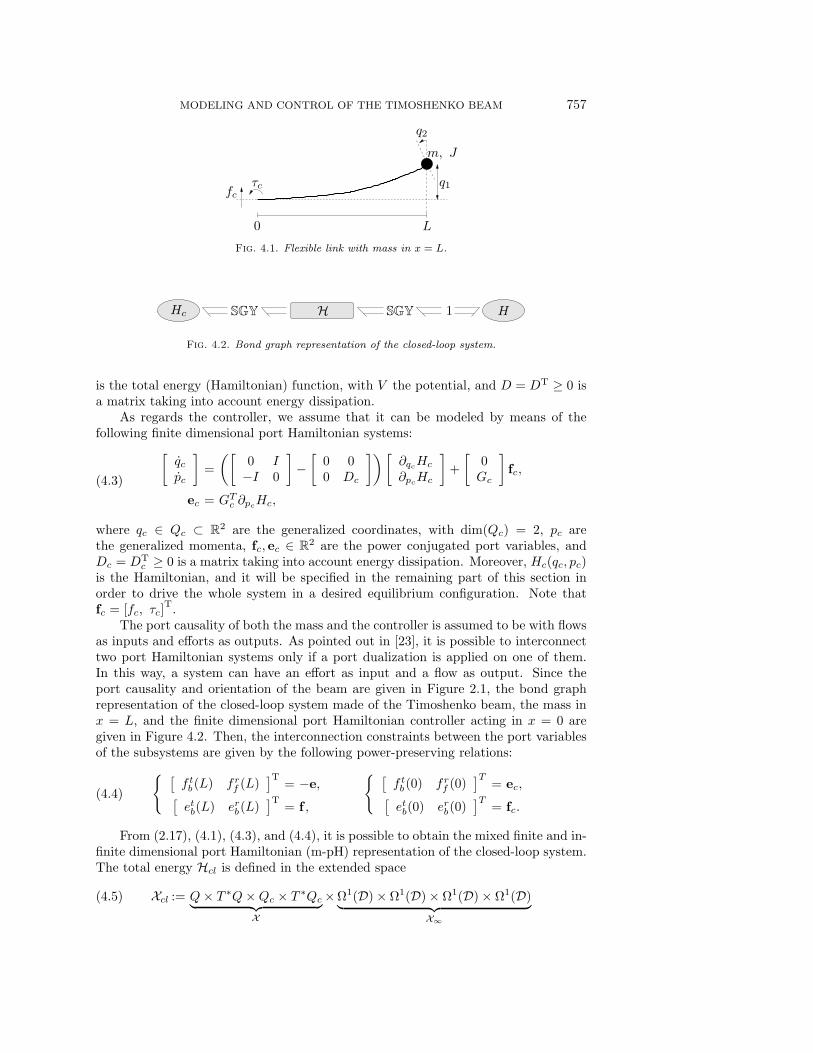
MODELING AND CONTROL OF THE TIMOSHENKO BEAM 757
0 L
q1
q2
m, J
fcτc
Fig. 4.1. Flexible link with mass in x = L.
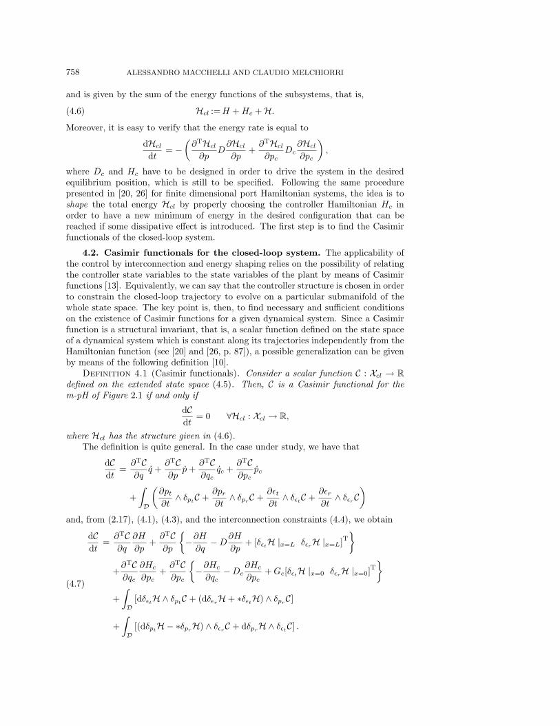
H HHc SGYSGY 1
Fig. 4.2. Bond graph representation of the closed-loop system.
is the total energy (Hamiltonian) function, with V the potential, and D = DT ≥ 0 isa matrix taking into account energy dissipation.
As regards the controller, we assume that it can be modeled by means of thefollowing finite dimensional port Hamiltonian systems:[
qcpc
]=
([0 I−I 0
]−[
0 00 Dc
])[∂qcHc
∂pcHc
]+
[0Gc
]fc,
ec = GTc ∂pcHc,
(4.3)
where qc ∈ Qc ⊂ R2 are the generalized coordinates, with dim(Qc) = 2, pc are
the generalized momenta, fc, ec ∈ R2 are the power conjugated port variables, and
Dc = DTc ≥ 0 is a matrix taking into account energy dissipation. Moreover, Hc(qc, pc)
is the Hamiltonian, and it will be specified in the remaining part of this section inorder to drive the whole system in a desired equilibrium configuration. Note thatfc = [fc, τc]
T.
The port causality of both the mass and the controller is assumed to be with flowsas inputs and efforts as outputs. As pointed out in [23], it is possible to interconnecttwo port Hamiltonian systems only if a port dualization is applied on one of them.In this way, a system can have an effort as input and a flow as output. Since theport causality and orientation of the beam are given in Figure 2.1, the bond graphrepresentation of the closed-loop system made of the Timoshenko beam, the mass inx = L, and the finite dimensional port Hamiltonian controller acting in x = 0 aregiven in Figure 4.2. Then, the interconnection constraints between the port variablesof the subsystems are given by the following power-preserving relations: [
f tb(L) fr
f (L)]T
= −e,[etb(L) erb(L)
]T= f ,
[f tb(0) fr
f (0)]T
= ec,[etb(0) erb(0)
]T= fc.
(4.4)
From (2.17), (4.1), (4.3), and (4.4), it is possible to obtain the mixed finite and in-finite dimensional port Hamiltonian (m-pH) representation of the closed-loop system.The total energy Hcl is defined in the extended space
Xcl := Q× T ∗Q×Qc × T ∗Qc︸ ︷︷ ︸X
×Ω1(D) × Ω1(D) × Ω1(D) × Ω1(D)︸ ︷︷ ︸X∞
(4.5)
758 ALESSANDRO MACCHELLI AND CLAUDIO MELCHIORRI
and is given by the sum of the energy functions of the subsystems, that is,
Hcl :=H + Hc + H.(4.6)
Moreover, it is easy to verify that the energy rate is equal to
dHcl
dt= −
(∂THcl
∂pD∂Hcl
∂p+
∂THcl
∂pcDc
∂Hcl
∂pc
),
where Dc and Hc have to be designed in order to drive the system in the desiredequilibrium position, which is still to be specified. Following the same procedurepresented in [20, 26] for finite dimensional port Hamiltonian systems, the idea is toshape the total energy Hcl by properly choosing the controller Hamiltonian Hc inorder to have a new minimum of energy in the desired configuration that can bereached if some dissipative effect is introduced. The first step is to find the Casimirfunctionals of the closed-loop system.
4.2. Casimir functionals for the closed-loop system. The applicability ofthe control by interconnection and energy shaping relies on the possibility of relatingthe controller state variables to the state variables of the plant by means of Casimirfunctions [13]. Equivalently, we can say that the controller structure is chosen in orderto constrain the closed-loop trajectory to evolve on a particular submanifold of thewhole state space. The key point is, then, to find necessary and sufficient conditionson the existence of Casimir functions for a given dynamical system. Since a Casimirfunction is a structural invariant, that is, a scalar function defined on the state spaceof a dynamical system which is constant along its trajectories independently from theHamiltonian function (see [20] and [26, p. 87]), a possible generalization can be givenby means of the following definition [10].
Definition 4.1 (Casimir functionals). Consider a scalar function C : Xcl → R
defined on the extended state space (4.5). Then, C is a Casimir functional for them-pH of Figure 2.1 if and only if
dCdt
= 0 ∀Hcl : Xcl → R,
where Hcl has the structure given in (4.6).The definition is quite general. In the case under study, we have that
dCdt
=∂TC∂q
q +∂TC∂p
p +∂TC∂qc
qc +∂TC∂pc
pc
+
∫D
(∂pt∂t
∧ δptC +∂pr∂t
∧ δprC +∂εt∂t
∧ δεtC +∂εr∂t
∧ δεrC)
and, from (2.17), (4.1), (4.3), and the interconnection constraints (4.4), we obtain
dCdt
=∂TC∂q
∂H
∂p+
∂TC∂p
−∂H
∂q−D
∂H
∂p+ [δεtH |x=L δεrH |x=L]
T
+∂TC∂qc
∂Hc
∂pc+
∂TC∂pc
−∂Hc
∂qc−Dc
∂Hc
∂pc+ Gc[δεtH |x=0 δεrH |x=0]
T
+
∫D
[dδεtH ∧ δptC + (dδεrH + ∗δεtH) ∧ δpr
C]
+
∫D
[(dδptH− ∗δpr
H) ∧ δεrC + dδprH ∧ δεtC] .
(4.7)
MODELING AND CONTROL OF THE TIMOSHENKO BEAM 759
The integral term in (4.7) is equal to∫D
[d (δεtH ∧ δptC) + d (δεrH ∧ δprC) + d (δptH ∧ δεtC) + d (δprH ∧ δεrC)]
−∫D
[δptH ∧ dδεtC + δprH ∧ (dδεrC + ∗δεtC)]
−∫D
[δεtH ∧ (dδptC − ∗δpr
C) + δεrH ∧ dδprC] ,
(4.8)
where, from the Stokes theorem, the first term can be written as∫∂D
[δεtH |∂D ∧δptC |∂D + · · · + δpr
H |∂D ∧δεrC |∂D]
=
∫∂D
[δpt
C |∂D δprC |∂D
] [δεtH |∂D δεrH |∂D
]T+
∫∂D
[δεtC |∂D δεrC |∂D
] [δptH |∂D δprH |∂D
]T.
(4.9)
From (4.1) and (4.3) and the interconnection constraints (4.4), we have that[δptH |x=L
δprH |x=L
]= −e = −∂H
∂pand
[δptH |x=0
δprH |x=0
]= ec = GT
c
∂Hc
∂pc.
Then, combining (4.7) with (4.8) and (4.9), we obtain that
dCdt
= −∂TC∂p
∂H
∂q− ∂TC
∂pc
∂Hc
∂qc
−−∂TC
∂q+
∂TC∂p
D +[δεtC |x=L δεrC |x=L
] ∂H
∂p
−−∂TC
∂qc+
∂TC∂pc
Dc +[δεtC |x=0 δεrC |x=0
]GT
c
∂Hc
∂pc
+
∂TC∂p
+[δpt
C |x=L δprC |x=L
] [δεtH |x=L δεrH |x=L
]T+
∂TC∂pc
−[δptC |x=0 δprC |x=0
] [δεtH |x=0 δεrH |x=0
]T−∫D
[δptH ∧ dδεtC + δprH ∧ (dδεrC + ∗δεtC)]
−∫D
[δεtH ∧ (dδptC − ∗δprC) + δεrH ∧ dδprC]
has to be equal to zero for every Hamiltonian H, Hc, and H (see Definition 4.1). Thisis true if and only if
dδεtC = 0, dδptC − ∗δprC = 0,dδεrC + ∗δεtC = 0, dδpr
C = 0,
∂C∂p
= 0,∂C∂pc
= 0,
[δpt
C |x=L
δprC |x=L
]= 0,
[δpt
C |x=0
δprC |x=0
]= 0,
∂C∂q
=
[δεtC |x=L
δεrC |x=L
],
∂C∂qc
= Gc
[δεtC |x=0
δεrC |x=0
].
(4.10)
760 ALESSANDRO MACCHELLI AND CLAUDIO MELCHIORRI
In other words, the following proposition has been proved [11, 12].Proposition 4.2. Consider the m-pH system of Figure 4.2, that is, the result
of the power conserving interconnection (4.4) of the subsystems (2.17), (4.1), and(4.3). If X × X∞ is the extended state space of the system, introduced in (4.5), thena functional C : X × X∞ → R is a Casimir for the closed-loop system if and only ifconditions (4.10) hold.
Since the necessary and sufficient conditions for the existence of Casimir functionshave been deduced, the control problem can be approached.
4.3. Control by energy shaping of the Timoshenko beam. In order tocontrol the flexible beam with the finite dimensional controller (4.3), the first stepis to find Casimir functionals for the closed-loop system that can relate the statevariables of the controller q to the state variables that describe the configuration ofthe flexible beam and the mass connected to its extremity. In particular, we arelooking for some functionals Ci, i = 1, 2, such that
Ci(q, p, qc, pc, pt, pr, εt, εr) := qc,i − Ci(q, p, pc, pt, pr, εt, εr) with i = 1, 2
are Casimir functionals for the closed-loop system, i.e., satisfying the conditions ofProposition 4.2.
First of all, from (4.10), we note immediately that every Casimir functional cannotdepend on p and pc. Moreover, since it is necessary that dδεtCi = 0 and dδpr
Ci = 0,we deduce that δεtCi and δpr
Ci have to be constant as a function on x on D andtheir value will be determined by the boundary conditions on Ci. Since, from (4.3),δprCi |∂D= 0, we deduce that δprCi = 0 on D. Since dδptCi = ∗δprCi = 0, then, fromthe boundary conditions, we deduce that also δpt
Ci = 0 on D. As a consequence,all the admissible Casimir functionals are also independent from pt and pr. In otherwords, we are interested in finding Casimir functionals in the following form:
Ci(q, qc, εt, εr) := qc,i − Ci(q, εt, εr), i = 1, 2.
Assuming Gc = I, we have that
∂C1
∂qc=
[10
]=
[δεtC1 |x=0
δεrC1 |x=0
](4.11)
and, consequently, δεtC1 = 1 on D. From (4.10), we have that dδεrC1 = −∗δεtC1 =−∗1 = −dx; then, δεrC1 = −x+c1, where c1 is determined by the boundary conditions.Since, from (4.11), δεrC1 |x=0= 0, then c1 = 0; moreover, we deduce that δεrC |x=L=−L, i.e., a new boundary condition in x = L. A consequence is that
∂C1
∂q=
[δεtC1 |x=L
δεrC1 |x=L
]=
[1−L
].
The first conclusion is that
C1(q, qc, εt, εr) = qc,1 − (Lq2 − q1) −∫D
(xεr − εt)(4.12)
is a Casimir for the closed-loop system. Following the same procedure, it is possibleto calculate C2. From (4.10), we have that
∂C2
∂qc=
[01
]=
[δεtC2 |x=0
δεrC2 |x=0
],

MODELING AND CONTROL OF THE TIMOSHENKO BEAM 761
and then δεtC2 = 0 on D; moreover, dδεrC2 = 0 and, consequently, δεrC2 = 1 on Dsince (4.6) holds. Again from (4.10), we deduce that
∂C2
∂q=
[δεtC2 |x=L
δεrC2 |x=L
]=
[01
].
So we can state that
C2(q, qc, εt, εr) = qc,2 + q2 +
∫Dεr(4.13)
is another Casimir functional for the closed-loop system. In conclusion, the followingproposition has been proved [11, 12].
Proposition 4.3. Consider the m-pH system of Figure 4.2, that is, the result ofthe power conserving interconnection (4.4) of the subsystems (2.17), (4.1), and (4.3).Then (4.12) and (4.13) are Casimir functionals for this system.
Note 4.1. Since Ci, i = 1, 2, are Casimir functionals, they are invariant for thesystem of Figure 4.2. Then, for every energy function Hc of the controller, we havethat
qc,1 = (Lq2 − q1) +
∫D
(xεr − εt) + C1, qc,2 = −q2 −∫Dεr + C2,(4.14)
where C1 and C2 depend on the initial conditions. If the initial configuration of thesystem is known, then it is possible to assume these constants are equal to zero. SinceHc is an arbitrary function of qc, it is possible to shape the total energy function of theclosed-loop system in order to have a minimum of energy in a desired configuration: ifsome dissipation effect is present, the new equilibrium configuration will be reached.
Suppose that the potential energy V in (4.2) is equal to
V (q1, q2) :=1
2
(k1q
21 + k2q
22
)(4.15)
with k1, k2 > 0. In other words, suppose that a translational and rotational springis acting on the rigid body in x = L. Furthermore, suppose that (q∗, 0), with
q∗ = [q∗1 q∗2 ]T, is the desired equilibrium configuration of the mass (4.1). Then, the
corresponding equilibrium configuration of the beam can be calculated as the solutionof (2.17) with
∂pt∂t
=∂pr∂t
=∂εt∂t
=∂εr∂t
= 0 on D
and with boundary conditions (in x = L) given by[f tb(L)
frb (L)
]=
∂H
∂p(q∗, 0) = 0,
[etb(L)erb(L)
]=
∂H
∂q(q∗, 0) =
[k1q
∗1
k2q∗2
].(4.16)
From (2.17), we have that the equilibrium configuration has to satisfy the followingsystem of PDEs:
dδεtH = 0,
∗δεtH + dδεrH = 0,
762 ALESSANDRO MACCHELLI AND CLAUDIO MELCHIORRI
whose solution, compatible with the boundary conditions (4.16), is equal to⎧⎪⎨⎪⎩
εt∗(x, t) =
k1
Kq∗1 ,
εr∗(x, t) =
k1q∗1
EI(L− x) +
k2q∗2
EI.
(4.17)
Furthermore, at the equilibrium, it is easy to compute that pt = pt∗ = 0 and that
pr = pr∗ = 0. From (4.14) and (4.17), define
q∗c,1 = qc,1(q∗1 , q
∗2 , εt
∗, εr∗) = Lq∗2 − q∗1 +
∫ L
0
(xεr∗ − εt
∗) dx
= Lq∗2 − q∗1 +
∫ L
0
[k1q
∗1
EI(L− x)x +
k2q∗2
EIx− k1
Kq∗1
]dx
=
(k1
EI
L3
6− k1
KL− 1
)q∗1 +
(k2
EI
L2
2+ L
)q∗2 ,
q∗c,2 = qc,2(q∗2 , εr
∗) = −q∗2 −∫ L
0
εrdx
= −q∗2 −∫ L
0
[k1q
∗1
EI(L− x) +
k2q∗2
EI
]dx = − k1
EI
L2
2q∗1 −
(k2
EIL + 1
)q∗2 .
Note that, at the equilibrium, pc = p∗c = 0. The energy function Hc of the controller(4.3) will be developed in order to regulate the closed-loop system in the configuration
χ∗ = (q∗, p∗, p∗c , pt∗, pr
∗, εt∗, εr
∗).
In the remaining part of this section it will be proved that, by choosing the controllerenergy as
Hc(pc, qc) =1
2pTc M
−1c pc +
1
2Kc,1(qc,1 − q∗c,1)
2 +1
2Kc,2(qc,2 − q∗c,2)
2
+Ψ1(qc,1) + Ψ(qc,2)
(4.18)
with Mc = MTc > 0, Kc,1,Kc,1 > 0, and Ψ1,Ψ2 functions still to be specified, the
configuration χ∗ is stable.Remark 4.1. It is important to point out that the proposed control methodology
is solution free; that is, a stabilizing controller is provided by (4.3) and (4.18) but theproblem of the existence of a solution of the PDE modeling the Timoshenko beamis not approached. As discussed in [9, Example 5.6], the Timoshenko beam equationgenerates a contraction semigroup; thus the equation has a unique classical solution.Furthermore, when closing the loop, what we obtain is a hybrid system, that is, asystem consisting of a coupled PDE with an ODE, and also in this case it should benecessary to check under which conditions a classical solution exists. The problem canbe solved by extending the approach proposed in [9, section 4.6.1], for the boundarycontrol of an Euler–Bernoulli beam by means of a PI + strain feedback controller, tothe case discussed in this paper.
As in the case of a finite dimensional Hamiltonian system, the stability of anm-pH system can be proved if it can be shown that the equilibrium is a strict extremumof the total energy of the closed-loop system. The only difference is that, in order

MODELING AND CONTROL OF THE TIMOSHENKO BEAM 763
to prove the stability for the infinite dimensional part, it is necessary to fix a norm:it is important to note that the stability with respect to this norm, in general, willnot assure the stability with respect to a different one (see, e.g., [24, p. 114]). Thestability definition in the sense of Lyapunov for mixed finite and infinite dimensionalsystems can be given as follows [24, Definition 4.18].
Definition 4.4 (Lyapunov stability for mixed systems). The equilibrium con-figuration χ∗ for a mixed finite and infinite dimensional system is said to be stable inthe sense of Lyapunov with respect to the norm ‖·‖ if, for every ε > 0, there existsδε > 0 such that
‖χ(0) − χ∗‖ < δε ⇒ ‖χ(t) − χ∗‖ < ε
∀t > 0, where χ(0) is the initial configuration of the system.As proposed in [24, pp. 116–117] and in [22], in order to verify the stability of χ∗,
it is necessary to show that it is an extremum of the closed-loop energy function Hcl
introduced in (4.6), with Hc given by (4.18); that is, the condition
∇Hcl(χ∗) = 0(4.19)
must hold. Moreover, if ∆χ is the displacement from the equilibrium configurationχ∗, introduce the nonlinear functional
N (∆χ) :=Hcl(χ∗ + ∆χ) −Hcl(χ
∗)(4.20)
that is proportional to the second variation of Hcl. Then the configuration χ∗ is stableif it is possible to find γ1, γ2, α > 0 such that [24, Theorem 4.20]
γ1 ‖∆χ‖2 ≤ N (∆χ) ≤ γ2 ‖∆χ‖α .(4.21)
Denote by χ the state variable of the closed-loop system. From (2.8), (4.2), (4.15),and (4.18), the total energy function is given by
Hcl(χ) =1
2
(p21
m+
p22
J
)+
1
2
(k1q
21 + k2q
22
)+
1
2
∫D
(1
ρpt ∧ ∗pt +
1
Iρpr ∧ ∗pr + Kεt ∧ ∗εt + EIεr ∧ ∗εr
)
+1
2pTc M
−1c pc +
1
2Kc,1(qc,1 − q∗c,1)
2 +1
2Kc,2(qc,2 − q∗c,2)
2
+Ψ1(qc,1) + Ψ(qc,2).
The first step in the stability proof is to find under which conditions, that is, for whatparticular choice of the functions Ψ1 and Ψ2, relation (4.19) is satisfied. We have that
∇Hcl(χ) =
⎡⎢⎢⎢⎢⎢⎢⎣
∂pHcl
∂qHcl
δptHcl
δprHcl
δεtHcl
δεrHcl
⎤⎥⎥⎥⎥⎥⎥⎦ =
⎡⎢⎢⎢⎢⎢⎢⎣
∂pH∂q(H + Hc)
δptHδprH
δεt(H + Hc)δεr (H + Hc)
⎤⎥⎥⎥⎥⎥⎥⎦ .

764 ALESSANDRO MACCHELLI AND CLAUDIO MELCHIORRI
Clearly,
∂H
∂p(χ∗) = 0,
∂Hc
∂pc(χ∗) = 0, δpt
H(χ∗) = 0, and δprH(χ∗) = 0.
Furthermore,
∂Hcl
∂q1= k1q1 −Kc,1
(qc,1 − q∗c,1
)− ∂Ψ1
∂qc,1,
∂Hcl
∂q2= k2q2 + Kc,1
(qc,1 − q∗c,1
)L−Kc,2
(qc,2 − q∗c,2
)+
∂Ψ1
∂qc,1L− ∂Ψ2
∂qc,2,
and
δεtHcl = K∗εt −Kc,1
(qc,1 − q∗c,1
)− ∂Ψ1
∂qc,1,
δεrHcl = EI∗εr + Kc,1
(qc,1 − q∗c,1
)x−Kc,2
(qc,2 − q∗c,2
)+
∂Ψ1
∂qc,1x− ∂Ψ2
∂qc,2.
Then ∇Hcl(χ∗) = 0 if
Ψ1(qc,1) = k1q∗1qc,1 + ψc,1,
Ψ2(qc,2) = (k2q∗2 + k1q
∗1L) qc,2 + ψc,2,
with ψc,1 and ψc,2 arbitrary constants. Once the equilibrium is assigned in χ∗, it isnecessary to verify the convexity condition (4.21) in χ∗ on the nonlinear functionalN . After simple calculations, it can be obtained (see [10]) that
‖∆χ‖ =1
2∆pTM−1∆p +
1
2∆pT
c M−1c ∆pc +
1
2k1∆q2
1 +1
2k2∆q2
2
+1
2
∫ L
0
(1
ρ∆pt ∧ ∗pt +
1
Iρ∆pr ∧ ∗pr + K∆εt ∧ ∗∆εt + EI∆εr ∧ ∗∆εr
)
+1
2Kc,1
[L∆q2 − ∆q1 +
∫ L
0
(x∆εr − ∆εt)
]2
+1
2Kc,2
[∆q2 +
∫ L
0
∆εr
]2
.
The convexity condition (4.21) requires a norm in order to be verified: a possiblechoice can be
‖χ‖2=
1
2∆pT∆p +
1
2∆pT
c ∆pc +1
2∆q2
1 +1
2∆q2
2
+1
2
∫ L
0
(∆pt ∧ ∗pt + ∆pr ∧ ∗pr + ∆εt ∧ ∗∆εt + ∆εr ∧ ∗∆εr) .
Then, in (4.21), assume that
γ1 =1
2min
|M−1|, |M−1
c |, k1, k2,1
ρ,
1
Iρ, K, EI
.
Moreover, if
γ2 =1
2max
|M−1|, |M−1
c |, k1, k2,1
ρ,
1
Iρ, K, EI, Kc,1, Kc,2
,
MODELING AND CONTROL OF THE TIMOSHENKO BEAM 765
we have that
N (∆χ) ≤ γ2 ‖∆χ‖+ γ2
[L∆q2 − ∆q1 +
∫ L
0
(x∆εr − ∆εt)
]2
+ γ2
[∆q2 +
∫ L
0
∆εr
]2
.
Since
[L∆q2 − ∆q1 +
∫ L
0
(x∆εr − ∆εt)
]2
≤ 2 (L∆q2 − ∆q1)2
+ 2
[∫ L
0
(x∆εr − ∆εt)
]2
≤ 4(|∆q1|2 + L2|∆q2|2
)+ 4
(∫ L
0
x∆εr
)2
+ 4
(∫ L
0
∆εt
)2
≤ 4(|∆q1|2 + L2|∆q2|2
)+ 4L
(∫ L
0
∆εt ∧ ∗∆εt + L
∫ L
0
∆εr ∧ ∗∆εr
),
[∆q2 +
∫ L
0
∆εr
]2
≤ 2|∆q2|2 + 2
(∫ L
0
∆εr
)2
≤ 2|∆q2|2 + 2L
∫ L
0
∆εr ∧ ∗∆εr,
it is possible to satisfy (4.21) by choosing α = 2 and
γ2 = γ2 · max4, 4L2 + 2, 4L, 4L2 + 2L
,
which completes the stability proof. In other words, the following proposition hasbeen proved.
Proposition 4.5. Consider the m-pH system of Figure 4.2, that is, the result ofthe power conserving interconnection (4.4) of the subsystems (2.17), (4.1), and (4.3).If in (4.3) it is assumed that Gc = I and Hc is chosen according to (4.18), then theconfiguration χ∗ is stable in the sense of Lyapunov, i.e., in the sense of Definition 4.4.
5. Conclusions. Once the Timoshenko model of the beam has been reformu-lated within the framework of dpH systems, some considerations about control strate-gies of the flexible beam have been presented. In particular, the well-known control bydamping injection is extended to distributed parameter systems in order to stabilizethe beam acting through its boundary and/or its distributed port. Some well-knownresults already presented in the literature are obtained in this new framework.
Moreover, it has been shown that it is possible to extend the energy shaping byinterconnection control technique to treat mixed finite and infinite dimensional sys-tems following the same ideas presented in [22], of which this work is a continuation.In particular, the control of a mechanical system made of a flexible beam with a rigidbody connected at one of its extremities has been presented. The finite dimensionalcontroller, acting on the system through the other extremity, is developed by prop-erly extending the concept of Casimir functions to infinite dimensions. The mainadvantage is that the controller is suitable for a clear physical interpretation, with thedrawback that the whole approach is solution free, in the sense of Remark 4.1.
Future work will deal with the extension of these concepts to the modeling andcontrol of simple kinematic chains with flexible links.
766 ALESSANDRO MACCHELLI AND CLAUDIO MELCHIORRI
REFERENCES
[1] C. I. Byrnes, A. Isidori, and J. C. Willems, Passivity, feedback equivalence, and the globalstabilization of minimum phase nonlinear systems, IEEE Trans. Automat. Control, 36(1991), pp. 1228–1240.
[2] T. J. Courant, Dirac manifolds, Trans. Amer. Math. Soc., 319 (1990), pp. 631–661.[3] R. F. Curtain and H. J. Zwart, An Introduction to Infinite Dimensional Linear Systems
Theory, Texts in Appl. Math. 21, Springer-Verlag, New York, 1995.[4] M. Dalsmo and A. J. van der Schaft, On representations and integrability of mathematical
structures in energy-conserving physical systems, SIAM J. Control Optim., 37 (1999),pp. 54–91.
[5] S. Dong-Hua and F. De-Xing, Exponential stabilization of the Timoshenko beam with locallydistributed feedback, in Proceedings of the 14th IFAC World Congress, Beijing, People’sRepublic of China, H. F. Chen, D.-Z. Cheng, and J.-F. Zhang, eds., Elsevier, New York,1999.
[6] G. Golo, V. Talasila, and A. J. van der Schaft, A Hamiltonian formulation of the Tim-oshenko beam model, in Proceedings of Mechatronics 2002, University of Twente, TheNetherlands, 2002, pp. 544–553.
[7] G. Golo, A. J. van der Schaft, and S. Stramigioli, Hamiltonian formulation of planarbeams, in Proceedings of the 2nd IFAC Workshop on Lagrangian and Hamiltonian Methodsfor Nonlinear Control, A. Astolfi, A. J. van der Schaft, and F. Gordillo, eds., Sevilla, Spain,Elsevier, New York, 2003, pp. 169–174.
[8] J. U. Kim and Y. Renardy, Boundary control of the Timoshenko beam, SIAM J. Control.Optim., 25 (1987), pp. 1417–1429.
[9] Z. H. Luo, B. Z. Guo, and O. Morgul, Stability and Stabilization of Infinite DimensionalSystems with Applications, Communications and Control Engineering Series, Springer-Verlag, London, 1999.
[10] A. Macchelli, Port Hamiltonian Systems. A Unified Approach for Modeling and ControlFinite and Infinite Dimensional Physical Systems, Ph.D. thesis, University of Bologna –DEIS, Bologna, Italy, 2003. Available at http://www-lar.deis.unibo.it/woda/data/deis-lar-publications/e499.Document.pdf
[11] A. Macchelli and C. Melchiorri, Control by interconnection of the Timoshenko beam, inProceedings of the 2nd IFAC Workshop on Lagrangian and Hamiltonian Methods for Non-linear Control, 2003, pp. 175–182.
[12] A. Macchelli and C. Melchiorri, Distributed port Hamiltonian formulation of the Tim-oshenko beam: Modeling and control, in Proceedings of the 4th MATHMOD, Vienna,Austria, 2003.
[13] J. E. Marsden and T. S. Ratiu, Introduction to Mechanics and Symmetry, Springer-Verlag,New York, 1994.
[14] J. E. Marsden and T. S. Ratiu, Geometry of Nonlinear Systems, 2001. This book is freelyavailable at http://www.cds.caltech.edu/∼marsden.
[15] B. M. Maschke and A. J. van der Schaft, Port controlled Hamiltonian systems: Model-ing origins and system theoretic properties, in Proceedings of the Third Conference onNonlinear Control Systems (NOLCOS), Bordeaux, France, 1992.
[16] B. M. Maschke and A. J. van der Schaft, Interconnection of systems: The networkparadigm, in Proceedings of the 35th IEEE Conference on Decision and Control, NewYork, 1996, pp. 207–212.
[17] B. M. Maschke and A. J. van der Schaft, Port controlled Hamiltonian representation ofdistributed parameter systems, in Workshop on Modeling and Control of Lagrangian andHamiltonian Systems, Princeton, NJ, 2000.
[18] B. M. Maschke and A. J. van der Schaft, Fluid dynamical systems as Hamiltonian boundarycontrol systems, in Proceedings of the 40th IEEE Conference on Decision and Control,Vol. 5, Orlando, FL, 2001, pp. 4497–4502.
[19] P. J. Olver, Application of Lie Groups to Differential Equations, Springer-Verlag, New York,1993.
[20] R. Ortega, A. J. van der Schaft, B. M. Maschke, and G. Escobar, Energy-shapingof port-controlled Hamiltonian systems by interconnection, in Proceedings of the IEEEConference on Decision and Control, Vol. 2, Phoenix, AZ, 1999, pp. 1646–1651.
[21] R. Ortega, A. J. van der Schaft, B. M. Maschke, and G. Escobar, Interconnectionand damping assignment passivity-based control of port-controlled Hamiltonian systems,Automatica, 38 (2000), pp. 585–596.

MODELING AND CONTROL OF THE TIMOSHENKO BEAM 767
[22] H. Rodriguez, A. J. van der Schaft, and R. Ortega, On stabilization of nonlinear dis-tributed parameter port-controlled Hamiltonian systems via energy shaping, in Proceedingsof the 40th IEEE Conference on Decision and Control, Vol. 1, Orlando, FL, 2001, pp. 131–136.
[23] S. Stramigioli, Modeling and IPC Control of Interactive Mechanical Systems: A Coordinate-Free Approach, Springer-Verlag, London, 2001.
[24] G. E. Swaters, Introduction to Hamiltonian Fluid Dynamics and Stability Theory, Chapmanand Hall/CRC, London, 2000.
[25] S. W. Taylor, Boundary Control of the Timoshenko Beam with Variable Physical Character-istics, Technical report, University of Auckland, New Zealand, 1997.
[26] A. J. van der Schaft, L2-Gain and Passivity Techniques in Nonlinear Control, in Commu-nication and Control Engineering, Springer-Verlag, London, 2000.


![Vibration of Timoshenko Beam-Soil Foundation Interaction by …jsm.iau-arak.ac.ir/article_677316_9f91814aa7024a7daa258... · 2 days ago · span Timoshenko beam. Banerjee [15] investigated](https://img.pdfslide.us/doc/110x75/60c0f04fc2fd995b4c03c833/vibration-of-timoshenko-beam-soil-foundation-interaction-by-jsmiau-arakacirarticle6773169f91814aa7024a7daa258.jpg)