Harmonic Decomposition Tidal Analysis and Prediction · PDF fileof the tides in January 2010 hourly and predict for the whole days of 2012 ... Astronomical argument, harmonic ... explained

Research Journal of Environmental and Earth Sciences 5(7): 381-392, 2013 ISSN: 2041-0484; e-ISSN: 2041-0492 © Maxwell Scientific Organization, 2013 Submitted: March 04, 2013 Accepted: March 27, 2013 Published: July 20, 2013

Corresponding Author: Nasser Najibi, Shanghai Astronomical Observatory, Chinese Academy of Sciences, Shanghai 200030,

China 381

Harmonic Decomposition Tidal Analysis and Prediction Based on Astronomical

Arguments and Nodal Corrections in Persian Gulf, Iran

1, 2Nasser Najibi, 3Abbas Abedini and 4Reza Arab Sheibani 1Shanghai Astronomical Observatory, Chinese Academy of Sciences, Shanghai 200030, China

2University of Chinese Academy of Sciences, Beijing 100049, China 3Faculty of Aerospace Engineering and Geodesy, Institute of Geodesy,

University of Stuttgart, Stuttgart D-70174, Germany 4Department of Surveying and Geomatics Engineering, College of Engineering,

University of Tehran, Tehran 11155-4563, Iran Abstract: The establishment and maintenance of marine structures and near-shore constructions together require having sufficient and accurate information about sea level variations not only in the present time but also in the near future as a reliable prediction. It is therefore necessary to analyze and predict Mean Sea Level (MSL) for a specific time considering all possible effects which may modify the accuracy and precision of the results. This study presents tidal harmonic decomposition solutions based on the first and second method of solving the Fourier series to analyze of the tides in January 2010 hourly and predict for the whole days of 2012 year considering the astronomical arguments and nodal corrections in Bandar-e-Abbas, Kangan Port and Bushehr Port tide gauge stations located in the Persian Gulf at the South of Iran. Moreover the accurate predictions of Mean Tide Level (MTL) are provided for the entire of 2012 year in each tide gauge station by excluding the effects of astronomical arguments and nodal corrections due to their unreasonable destroying effects. The MTL's fluctuations derived from the predicted results during 2012 year and different phases of the Moon show a very good agreement together according to tide-generating forces theories. Keywords: Astronomical argument, harmonic decomposition, moon phases, nodal correction, tidal prediction, tide

gauge

INTRODUCTION

Tidal analysis and prediction are the initial steps in the studies of each hydrodynamic and coastal management issue. It is dealing with the scrutiny of the sea level heights observations using physical and geophysical methods developed from experiences or physical reasoning and based on spectral analysis (commonly Fourier series) (Doodson, 1954; Godin, 1972; Hendershott, 1977; Le Provost and Fornerino, 1985; Le Provost et al., 1991; Shum et al., 2001). The prediction is used in the science and engineering to confirm the understanding of a given phenomenon by stating what its behavior till now and will be at a given time and then verifying that it is so (Godin, 1972), while without considering the physical effects of the large events (e.g., tsunami, storms, seabed earthquake and so on) the prediction of water levels can achieve with much improvements than itself (Wyatt et al., 1982; Shum et al., 1997).

Although the pioneer of the numerical solution of ocean tides was based on Laplace shallow water equations as used in many initial tide analysis studies; for example in Hendershott (1977) and Franco (1981),

but since the harmonic decomposition solution method developed which provided a complete way to tidal analysis and prediction (Doodson, 1922, 1954), there are many further works and much progress into analyzing of sea levels and examine the accuracy of the solution through different approaches (liu et al., 1985; Iz and Shum, 2000; Lyard et al., 2006; Iz, 2006) e.g., the increasing precision of field observations has required corrections for tidal effects that could previously be ignored completely (Agnew, 1995, 1997). Not only the tides now are precisely known in the most global ocean, but we also have learned and quantified new aspects of tidal dynamics (Lyard et al., 2006).

There are many natural oil and gas sources throughout Persian Gulf where through Tang-e-Hormoz strait and then Oman Sea is connecting to Indian Ocean directly and thus it may be a very strategic place to analyze the tidal components especially sea level variations there. Besides, several off-shore and near-shore petroleum companies and suppliers have been established there, to be aware of the current status of sea level variations and predict them could be as an essential agenda in each of them.

Res. J. Environ. Earth Sci., 5(7): 381-392, 2013

382

However currently remote sensing techniques and space based missions would help us through providing with a dense coverage of data temporally and spatially, but due to the time limitations, in hand tools of measuring tides and incapability of satisfying accurate resolutions in small regions such as gulfs, rivers and straits; it is thus necessary to apply the classical tide analysis and prediction techniques.

In order to predict tidal components and sea level heights in a special period of time, many considerations should be taken account (Godin, 1972; Walters et al., 2001; Agnew, 2007). Even though several undesirable natural events may affect on the predictions, but still there are determinable parameters which are necessary to handle them precisely, e.g., astronomical arguments and nodal corrections are playing the significant roles in dealing with tidal analysis and prediction.

This study firstly presents briefly basic concepts of tide causes and theories in theory and methodology Section. Field observations and data collection’s section gives complete information about the data used in this study. In the results and discussion section, the sea level heights variations are represented during 2010 year in three tide gauge stations in the South of Iran at Persian Gulf titled Bandar-e-Abbas, Kangan Port and Bushehr Port station. Besides, the modeling of tidal time series based on harmonic decomposition for January 2010 is explained in detail for these three tide gauge stations in comparison to the real tidal gauge observations through first and second method solution approaches of Fourier series and the relevant residuals by Least Squares Solution (LSS). Moreover, the procedures to represent the sea level heights for 2012 year considering the astronomical arguments and nodal corrections are discussed completely with corresponding principal tidal components values for these stations in the tables and figures. Finally conclusion’s section is presenting the final summary and conclusions in order to indicate some possible methods and more useful techniques for this type of investigation.

THEORY AND METHODOLOGY

In general tides mean when the elastic surface of the Earth is deforming periodically due to gravitational forces of other planetary bodies especially the Sun and the Moon that are located in near distance of the Earth rather than the others (Doodson, 1922). The effects of these forces will result in mass redistribution of the Earth in large scale fluids including the oceans and huge seas by the changes in the geo-potential components. According to Newton’s law of gravitation, the ocean tides are generating by combinations of the traction effects of gravitational forces of the Sun and

the Moon as well as centrifugal forces coming from the Earth’s movements around the Sun and itself continuously (Agnew, 1986; Wang, 2004). Therefore, after simplifying the Newton’s law and considering the spherical triangle for each point of Re, and λ on the Earth’s surface, the potential of tide can be written as thus:

( ) ( ) ( )( ) ( ) ( ) ( )0

2 0

!, , 2 sin sin cos

!

l le

e m lm lml m

l mRGMU R P P mHR R l m

φ λ δ φ δ∞

= =

−⎛ ⎞= −⎜ ⎟ +⎝ ⎠∑ ∑

(1)

where Re : The mean radius of the Earth R : The geocentric distance

& λ : The geocentric latitude and the longitude of the location of the point on the Earth’s surface in the geodetic coordinate system

δ : The declination angle of point δ0m : The Kronecker delta H : The hour angle of the attracting body from the

point’s view (Re, , λ) Plm (sin ) & Plm (sin δ) : The associated Legendre

functions Following with the values of m = 0, 1 and 2 (according to Agnew (2007) only the term with l = 2 is mostly considered as the tide potential generation impact, however sometime l = 3 is also considered as the Moon impact’s factor for the tide generating potential) and by taking account that the sea or ocean surface is normal to the resultant of the Earth’s gravity and of the tidal generating forces, the Eq. (1) for l = 2 can be expressed as:

( ) ( )

2 222

2 2 30

2 2

cos cos cos 23, , , , sin 2 sin 2 cos

41(1 3sin )( sin )3

ee m e

m

HGMRU R U R H

R

φ δφ λ φ λ φ δ

φ δ=

⎧ ⎫⎪ ⎪+⎪ ⎪

= = + +⎨ ⎬⎪ ⎪⎪ ⎪+ − −⎩ ⎭

∑

(2) where with the same variable’s introduced in Eq. (1) and (2) separates the period of the lunar tidal potential into three terms with period of 12 h, 24 h and 14 days approximately. Similarly the solar tidal potential has periods of 12 h, 24 h and 180 days, respectively. Thus there are three distinguished collections of tidal frequencies; twice-daily (semi daily), daily and long period. Pertaining to the 2H (m = 2) and H (m = 1) components; the δcos2H represents the semi-diurnal term, sin2 δcosH is expressing diurnal term and the (1-3 ) ( - δ) can be interpreted as long-period term in the tide potential


383

analysis. Based on these basic equations and concepts, the harmonic tide decomposition will be discussed briefly. Moreover Astronomical argument and nodal corrections will be represented. In this study we have applied both harmonic tide decomposition and nodal corrections in the results and discussions of the tide gauge stations. Harmonic tide decomposition: The observations of water levels can be represented as the sequences through the form of:

{Z (t)} (3) where, Z (t) expresses the water level at the time of t. Doodson (1992) proposed Fourier series expansion instead of Eq. (2) and (3) applying fundamental tidal frequencies to interpret tidal constituents (also known as partial tides). Therefore, by simplicity the water level’s equations which can be written as:

0

01

( ) cos( ) sin( )

cos( ) sin( )

k

i i i ii

k

i i i ii

f t a w t b w t

a a w t b w t

=

=

= +

= + +

∑

∑

(4)

where, f (t) : Observation of water level at the time of t wi : Angular frequency of harmonic i (wi = 2π/T, T

is period of tide) ai & bi : The Fourier coefficients In order to compute the Mean Tide Level (MTL), we use Eq. (4) in two different cases; in the First Method the water wave has been removed from the sea water level observations during each step of applying the LSS to compute the Fourier coefficients as Eq. (5) and (7):

1 11

2 2 2

cos( ), sin( )( )( ) cos( ), sin( )

. .

. .

. .( ) cos( ), sin( )

k k

k k

k

k

k k k k k

w t w tf tf t w t w t

ab

f t w t w t

⎡ ⎤⎡ ⎤⎢ ⎥⎢ ⎥⎢ ⎥⎢ ⎥⎢ ⎥⎢ ⎥ ⎡ ⎤

= ⎢ ⎥⎢ ⎥ ⎢ ⎥⎣ ⎦⎢ ⎥⎢ ⎥

⎢ ⎥⎢ ⎥⎢ ⎥⎢ ⎥

⎢ ⎥ ⎢ ⎥⎣ ⎦ ⎣ ⎦

(5)

where, w and t as well as ai and bi have the same concepts introduced in Eq. (4).

Similarly in the Second Method in order to get the MTL, firstly all the Fourier coefficients are computing and then the principle waves of water (tidal heights) are excluding from the observations using Eq. (6) and (7); so that:

1

11 1 1 1 1 11

22 1 2 1 2 2 2

2

1 1

cos( ), sin( )...cos( ), sin( )( )( ) cos( ), sin( )...cos( ), sin( )

. ..

. ..

. ..

( ) cos( ), sin( )...cos( ), sin( )

k k

k k

k k k k k k kk

k

ab

w t w t w t w tf ta

f t w t w t w t w tb

f t w t w t w t w tab

⎡ ⎤⎡ ⎤⎢ ⎥⎢ ⎥⎢ ⎥⎢ ⎥⎢ ⎥⎢ ⎥

= ⎢ ⎥⎢ ⎥⎢ ⎥⎢ ⎥⎢ ⎥⎢ ⎥⎢ ⎥⎢ ⎥

⎢ ⎥ ⎢ ⎥⎣ ⎦ ⎣ ⎦

⎡ ⎤⎢ ⎥⎢ ⎥⎢ ⎥⎢ ⎥⎢ ⎥⎢ ⎥⎢ ⎥⎢ ⎥⎢ ⎥⎢ ⎥⎢ ⎥⎢ ⎥⎣ ⎦

(6)

where, w, t, ai and bi have the same definitions mentioned in Eq. (4 ) above. The difference between the precisions and residuals of these two methods will be discussed later in the results and discussions section by solving Eq. (7) and (8) as:

( ) 1ˆo T T oL AX V X A PA A PL−

= + → = (7)

ˆ oV AX L= − (8) where, in each solution of harmonic decomposition, Lo : Observed tidal heights (mentioned above as f (tk)) A : Includes the whole trigonometric terms X : Unknown terms which here are the Fourier

coefficients (ak, bk) V : Error’s term in general concept P : Weighted matrix based on precisions of

observations which we supposed the observations might have similar errors and equal to unique

Astronomical argument and nodal corrections: To consider the Doodson’s harmonic expansion to interpret tidal components as Fourier series, the tidal levels can then be expressed by a limit number of harmonics in the form of:

0( ) (0) ( ) cos( ( ) )

k

i i i i i ii

h t h S t a w t v u t g=

= + + + −∑

(9)

where, wi : The same term introduced in Eq. (4) h (0) : The mean height Si : Nodal correction value ai : The amplitude vi : Astronomical argument ui : The phase of nodal correction gi : The phase of lag on the equilibrium tide Obviously in Eq. (9), the ai and gi are unknown terms and need to be computed by performing LSS and h (0) is computed based on time series interpolation of the water level observations and the rest of the terms are available in the astronomical tables provided by Institute of Ocean Science (IOS) as given known


384

Fig. 1: Locations of tide gauge stations at south of Iran in Persian Gulf used in this study (Bandar-e-Abbas, Kangan Port and

Bushehr Port station)

Fig. 2: Comparison of astronomical arguments in January 1, 2010 (green vectors) and January 1, 2012 (red vectors)

Fig. 3: Comparison of nodal corrections values for principal tidal components in July 1, 2010 (green bars) and July 1, 2012 (red

bars) parameters specified to every area and local time. In this study, in order to predict the tide for entire 2012 year, the nodal corrections have been affected into the final results in the three case studies (three tide gauge stations).

Field observations and data collection: Tide gauge observations: Hourly sea level heights in three tide gauge stations located at Persian Gulf, Iran are used during January 2010. These tide stations are Bandar-e-Abbas, Kangan Port and Bushehr Port where

48oE 52oE 56oE 60oE 64oE 22oN

24oN

26oN

28oN

30oN

PERSIAN GULF

SAUDI ARABIA

Tide Gauge Stations in Persian Gulf

Kangan PortStation Bandar-e-Abbas

Station

Bushehr PortStation

OMAN SEA

INDIAN OCEAN

IRAN

-1 -0.8 -0.6 -0.4 -0.2 0 0.2 0.4 0.6 0.8 1-1

.8

.6

.4

.2

0

.2

.4

.6

.8

1

Astronomical Arguments in January 1, 2010 (green) and 2012 (red) [circular degree]

270 deg.

90 deg.

180 deg. 00 deg.

0 0.1 0.2 0.3 0.4 0.5 0.6 0.7 0.8 0.9 1 1.11.1

1

2

3

4

5

6

7

8

Q1

O1

P1

K1

N2

M2

S2

K2

Nodal Corrections in July 1, 2010 and 2012

2010 2012


385

Table 1: Astronomical argument in January 1, 2010 and 2012 and nodal corrections in July 1, 2010 and 2012 (Schureman, 1959)

Argument Year

Constituents [°degree] ----------------------------------------------------------------------------------------------------------------------------------------Q1 O1 P1 K1 N2 M2 S2 K2

Astronomical 2010 355.377 331.542 350.116 18.343 18.188 352.965 359.885 217.329Nodal corrections 1.068 1.054 0.996 1.038 0.993 0.993 1.001 1.076 Astronomical 2012 17.593 170.909 350.485 18.923 41.950 194.551 359.894 217.763Nodal corrections 0.914 0.941 1.006 0.961 1.014 1.016 0.999 0.893

Table 2: Main phases of the moon occurrence in the Universal Time (UT) during 2012 year Moon phases Clock times of the moon phases based on the UT at 00hour00minute

New moon - Jan. 23 Feb. 21 Mar. 22 Apr. 21 May 20 Jun. 19 Jul. 19 Aug. 17 Sep. 16 Oct. 15 Nov. 13 Dec. 13 07 39 22 35 14 37 07 18 23 47 15 02 04 24 15 54 02 11 12 02 22 08 08 42

First quarter Jan. 1 Jan. 31 Mar. 1 Mar. 30 Apr. 29 May 28 Jun. 27 Jul. 26 Aug. 24 Sep. 22 Oct. 22 Nov. 20 Dec. 20 06 15 04 10 01 21 19 41 09 57 20 16 03 30 08 56 13 54 19 41 03 32 14 31 05 19 Full moon Jan. 9 Feb. 7 Mar. 8 Apr. 6 May 6 Jun. 4 Jul. 3 Aug. 2 Aug. 31 Sep. 30 Oct. 29 Nov. 28 Dec. 28 07 30 21 54 09 39 19 19 03 35 11 12 18 52 03 27 13 58 03 19 19 49 14 46 10 21 Last quarter Jan. 16 Feb. 14 Mar. 15 Apr. 13 May 12 Jun. 11 Jul. 11 Aug. 9 Sep. 8 Oct. 8 Nov. 7 Dec. 6 - 09 08 17 04 01 25 10 50 21 47 10 41 01 48 18 55 13 15 07 33 00 36 15 31 the geographical locations of them are shown in Fig. 1. However the sea level heights once per four-hour (1st h, 3rd h and so on during 1 day) have been observed for the whole 2010 year, the tide gauge instruments existed in these stations could get sea level heights hourly with precision of 0.001 m. The sea level frequencies data and timely sea level heights of these three stations have been provided by National Centre of Cartography of Iran (NCCI). Astronomical and nodal corrections data: As it mentioned above, the astronomical arguments values are necessary in order to predict the tidal heights and amplitudes based on the current tide gauge observations Eq. (9). The values including astronomical arguments (for Q1, O1, P1, K1, N2, M2, S2 and K2 in degree) and the corresponding nodal corrections respectively have been derived from Institute of Ocean Sciences (IOS) (Table 1). Obviously the astronomical arguments and modal corrections are changing year by year mostly due to the inclination of the Earth’s rotation axis (Precession and Nutation motions) and different positions of the Earth moving around the Sun and itself. Figure 2 and 3 present the different between astronomical arguments and nodal corrections in January 1, 2010 comparing to January 1, 2012 respectively. Besides, the clock times of main phases of the moon occurrence (such as main moon, first quarter, full moon and last quarter) in the Universal Time (UT) during 2012 year are available in Table 2 (http://aa.usno.navy.mil/data/docs/MoonPhase.php, accessed on January 1, 2013).

We use tide gauge observations and astronomical arguments as well as the corresponding nodal corrections together to apply the First Method and Second Method of harmonic decomposition solutions in January 2010 and then predict the tides for 2012 year.

RESULTS AND DISCUSSION

In order to get the yearly time series variations of sea level in the stations including Bandar-e-Abbas, Kangan Port and Bushehr Port, the elevation of sea level must be measured in a rate of one hour by one hour during at least one month in the relevant tide gauge stations. The general procedure of analyzing tides in January 2010 and predicting them for 2012 year respect to nodal corrections and astronomical arguments is presented in Fig. 4 as a flowchart where it is starting from up by inserting of sea level observations and following in toward harmonic decomposition solution in First and Second Method approach and then affected by astronomical arguments and nodal corrections to get the time series prediction of tides for 2012 year in three tide gauge stations including Bandar-e-Abbas, Kangan Port and Bushehr Port.

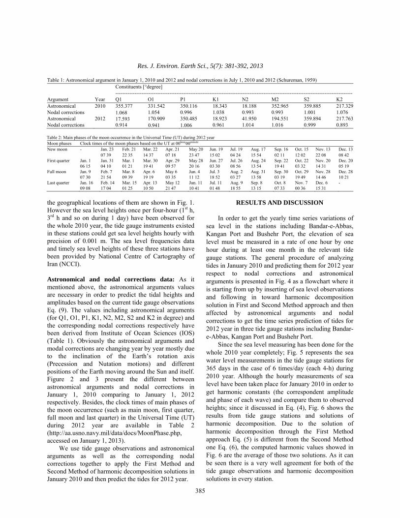
Since the sea level measuring has been done for the whole 2010 year completely; Fig. 5 represents the sea water level measurements in the tide gauge stations for 365 days in the case of 6 times/day (each 4-h) during 2010 year. Although the hourly measurements of sea level have been taken place for January 2010 in order to get harmonic constants (the correspondent amplitude and phase of each wave) and compare them to observed heights; since it discussed in Eq. (4), Fig. 6 shows the results from tide gauge stations and solutions of harmonic decomposition. Due to the solution of harmonic decomposition through the First Method approach Eq. (5) is different from the Second Method one Eq. (6), the computed harmonic values showed in Fig. 6 are the average of those two solutions. As it can be seen there is a very well agreement for both of the tide gauge observations and harmonic decomposition solutions in every station.

Fig. 4: Flow

astroGulf

wchart of tide aonomical argumf

0

1

2

3

4

5

6

Var

iatio

ns o

f sea

leve

l (m

)

0

1

2

3

4

Var

iatio

ns o

f sea

leve

l (m

)

Res.

analysis during ents effects in B

100 200

T

1s

100 200

1s

J. Environ. Ea

January 2010 Bandar-e-Abbas,

300 400Hourly

Tide Guage Yearly

st hr 3rd hr

300 400Hourly

Tide Guage Yea

st hr 3rd hr

arth Sci., 5(7):

386

and tide predic Kangan Port an

500 600y observations (20

y Obserrvations [B

5th hr 7th hr

500 600y observations (2

arly Obserrvations

5th hr 7th hr

381-392, 2013

ction for 2012 ynd Bushehr Port

700 800010)

Bandar-e-Abbas]

9th hr 11t

700 800010)

s [Kangan Port]

r 9th hr 11

3

year based on t tide gauge stati

900 1000

th hr

900 1000

th hr

nodal correctionions located in P

ns and Persian


387

Fig. 5: Variations of sea level heights observed each 4-h/day during 2010 year in Bandar-e-Abbas, Kangan Port, and Bushehr Port

100 200 300 400 500 600 700 800 900 10000

1

2

3

4

5

Hourly observations (2010)

Var

iatio

ns o

f sea

leve

l (m

)

Tide Guage Yearly Obserrvations [Bushehr Port]

1st hr 3rd hr 5th hr 7th hr 9th hr 11th hr

0 100 200 300 400 500 600 700

1

2

3

4

5

Hourly observations (January 2010)

Var

iatio

ns o

f sea

leve

l (m

)

Bandar-e-Abbas

Tide GaugeHarmonic Decomposition

0 100 200 300 400 500 600 7000

1

2

3

3.5


Var

iatio

ns o

f sea

leve

l (m

)

Kangan Port



388

Fig. 6: Comparison of sea levels between tide gauge observations and harmonic decomposition solutions during January 2010 for Bandar-e-Abbas, Kangan Port and Bushehr Port based on hourly observations

0 100 200 300 400 500 600 7001

2

3

4


Var

iatio

ns o

f sea

leve

l (m

)

Bushehr Port


0 100 200 300 400 500 600 700-4

-3

-2

-1

0

1

2

3

4First and Second Method Solution for Mean Tide Level [Bandar-e-Abbas]


Res

idua

ls (

m)

First Method Second Method

0 100 200 300 400 500 600 700-2

-1

0

1

2First and Second Method Solution for Mean Tide Level [Kangan Port]


Res

idua

ls (

m)



389

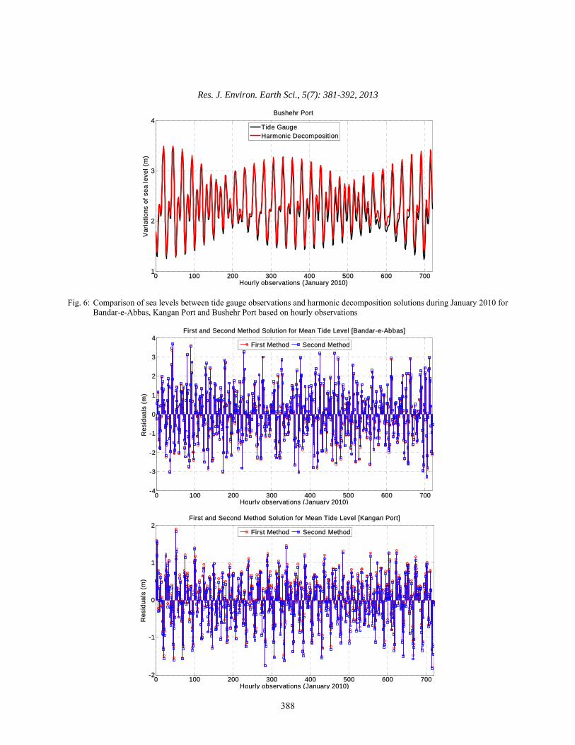
Fig. 7: The residuals of solution of first method and second method of harmonic decomposition for mean tide level during January 2010 for Bandar-e-Abbas, Kangan Port and Bushehr Port tide gauge stations

0 100 200 300 400 500 600 700-2

-1

0

1

2First and Second Method Solution for Mean Tide Level [Bushehr Port]


Res

idua

ls (

m)


0 2000 4000 6000 8000 8760

1

2

3

4

5

Hourly computations (2012)

Mea

n Ti

de L

evel

(M

TL)

[m]

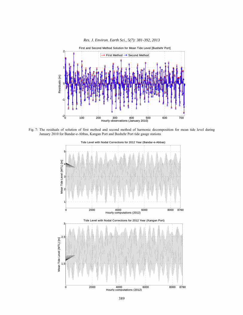
Tide Level with Nodal Corrections for 2012 Year (Bandar-e-Abbas)

0 2000 4000 6000 8000 8760

1.5

2.5

3


Mea

n Ti

de L

evel

(M

TL)

[m]

Tide Level with Nodal Corrections for 2012 Year (Kangan Port)


390

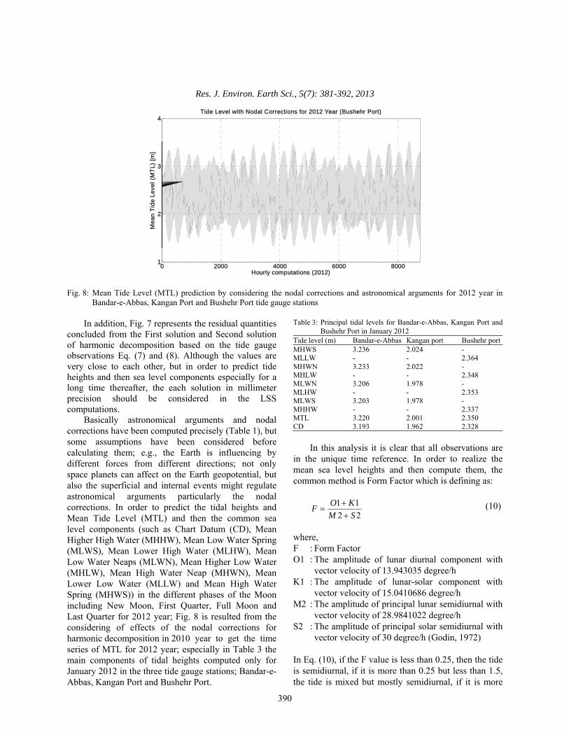
Fig. 8: Mean Tide Level (MTL) prediction by considering the nodal corrections and astronomical arguments for 2012 year in Bandar-e-Abbas, Kangan Port and Bushehr Port tide gauge stations

In addition, Fig. 7 represents the residual quantities

concluded from the First solution and Second solution of harmonic decomposition based on the tide gauge observations Eq. (7) and (8). Although the values are very close to each other, but in order to predict tide heights and then sea level components especially for a long time thereafter, the each solution in millimeter precision should be considered in the LSS computations.

Basically astronomical arguments and nodal corrections have been computed precisely (Table 1), but some assumptions have been considered before calculating them; e.g., the Earth is influencing by different forces from different directions; not only space planets can affect on the Earth geopotential, but also the superficial and internal events might regulate astronomical arguments particularly the nodal corrections. In order to predict the tidal heights and Mean Tide Level (MTL) and then the common sea level components (such as Chart Datum (CD), Mean Higher High Water (MHHW), Mean Low Water Spring (MLWS), Mean Lower High Water (MLHW), Mean Low Water Neaps (MLWN), Mean Higher Low Water (MHLW), Mean High Water Neap (MHWN), Mean Lower Low Water (MLLW) and Mean High Water Spring (MHWS)) in the different phases of the Moon including New Moon, First Quarter, Full Moon and Last Quarter for 2012 year; Fig. 8 is resulted from the considering of effects of the nodal corrections for harmonic decomposition in 2010 year to get the time series of MTL for 2012 year; especially in Table 3 the main components of tidal heights computed only for January 2012 in the three tide gauge stations; Bandar-e-Abbas, Kangan Port and Bushehr Port.

Table 3: Principal tidal levels for Bandar-e-Abbas, Kangan Port and Bushehr Port in January 2012

Tide level (m) Bandar-e-Abbas Kangan port Bushehr portMHWS 3.236 2.024 - MLLW - - 2.364 MHWN 3.233 2.022 - MHLW - - 2.348 MLWN 3.206 1.978 - MLHW - - 2.353 MLWS 3.203 1.978 - MHHW - - 2.337 MTL 3.220 2.001 2.350 CD 3.193 1.962 2.328

In this analysis it is clear that all observations are in the unique time reference. In order to realize the mean sea level heights and then compute them, the common method is Form Factor which is defining as:

1 12 2

O KFM S

+=

+ (10)

where, F : Form Factor O1 : The amplitude of lunar diurnal component with

vector velocity of 13.943035 degree/h K1 : The amplitude of lunar-solar component with

vector velocity of 15.0410686 degree/h M2 : The amplitude of principal lunar semidiurnal with

vector velocity of 28.9841022 degree/h S2 : The amplitude of principal solar semidiurnal with

vector velocity of 30 degree/h (Godin, 1972) In Eq. (10), if the F value is less than 0.25, then the tide is semidiurnal, if it is more than 0.25 but less than 1.5, the tide is mixed but mostly semidiurnal, if it is more

0 2000 4000 6000 80001

2

3

4


Mea

n Ti

de L

evel

(M

TL)

[m]

Tide Level with Nodal Corrections for 2012 Year (Bushehr Port)


391

than 1.5 and less than 3, then the tide is mixed but mostly diurnal and eventually if it is bigger than 3, then the tide is diurnal. Based on Eq. (10), the tide in Bandar-e-Abbas is mixed but mainly semidiurnal, in Kangan Port is mixed but mainly semidiurnal and in Bushehr Port is mixed but mainly diurnal in January 2010.

Moreover, there are many approaches to get the Chart Datum (CD). The long term tidal heights observations would give us more acceptable value for CD. Although in order to compute CD, at least monthly observations are necessary, but CD is very localized parameter depends on natural behavior of tides in that region. Until now several methods have been used by many hydrographical organizations around the world to get the CD, but the usual one is applying the equation of Indian Spring Low Water when the tide is semidiurnal or mostly semidiurnal as the following:

0 1.1( 1 1 2 2)CD Z O K M S= − + + + (11) where, Z0 : The average of water levels during

the collecting data O1, K1, M2 & S2 : The principal amplitude of

harmonic decomposition solution introduced in Eq. (10)

Note that when the tide is diurnal or mostly diurnal the coefficient of 1.1 in Eq. (11) should be removed. The CD for Bandar-e-Abbas, Kangan Port and Bushehr Port in January 2012, respectively is placed in Table 3.

Pertaining to the essential concepts of tidal generating forces and causes on the sea or ocean water levels around the Earth’s surface, Table 2 and Fig. 8 are in a very good agreement, so that the Moon’s phases especially New Moon and Full Moon are influencing the sea water levels strongly rather than the other phases of the Moon. Moreover, the effect of the Moon (due to be in the close distance of the Earth than the Sun) is more sensible in large water storages (oceans and wide seas) compare with small ones (e.g., shallow waters such as lakes, gulfs and rivers); for example the sea level variations are longer in Bandar-e-Abbas tide station than Kangan Port or Bushehr Port tide station. Kangan Port is located in Persian Gulf but Bandar-e-Abbas has less distance to India Ocean and thus can be affected its local geo-potential largely. Although this can be true whether the tide stations are locating nearby each other or the weather and the other environmental parameters should be equal for all of them.

However the errors introduced by applying nodal corrections for the time period of more than one month (e.g., for entire 2012 year) depend on the duration of

the time series and the considered LSS precisions, but they will increase with the decreasing of time period duration. It is very complicated situation due to distribution of different kinds of energy by several components and frequencies which some of them are more accurate than the others and it is not reasonable to define general rules to analyze the errors.

CONCLUSION

In this study, modeling and prediction of ocean

tides presented in the Persian Gulf at the South of Iran in three tide gauge stations including Bandar-e-Abbas, Kangan Port and Bushehr Port in detail for January 2010 and January 2012 as well as 2012 year entirely. As it mentioned, Persian Gulf is an important region and has a very critical role in the all Middle East countries and thus it is vital to focus on there. The effects of astronomical arguments and nodal corrections considered in the 2012 year MTL’s prediction which did not study in the most previous studies in this region. It should be kept in mind that differences between observed and predicted sea level parameters may vary due to the fact that in the prediction approach, the nodal correction value is calculated only for the central hour of the whole prediction time period. Moreover the residuals caused by solution of harmonic decomposition through two different approaches (First Method and Second Method) represented separately in each tide gauge station for January 2010. The comparison between the moon phases (Table 2) and the fluctuations of MTL in 2012 year (Fig. 8) shows the MTL’s values agree well with the moon phases. The comparison in terms of prediction of principal tidal levels in January 2012 between three tide stations as well as Fig. 1 demonstrate the distance between Bandar-e-Abbas and Kangan Port is less than between Bandar-e-Abbas and Bushehr Port station. Besides, Bandar-e-Abbas and Kangan Port stations have similar Form Factor rather than Bushehr Port station. Although applying the ground tidal heights observations are very common and in hand to analyze the tides modeling and predict them for a given time, but remote sensing techniques such as satellite missions and space based sensors can help us to get the sea level observations with larger spatial and temporal coverage even in special regions (e.g., polar regions) for hydrodynamic studies and coastal managements (Mayer-Gürr et al., 2012). Therefore, the tidal challenge and its solutions have not yet terminated; whereas the future models will need to improve the current tidal solutions and predictions in local or globally; particularly in the coastal and shelf regions where the objective of existence the narrowing disruption between the shallow water and deep ocean and their range of prediction accuracy.


392

ACKNOWLEDGMENT

The authors would like to thank National Cartographic Center of Iran (NCC) and Institute of Ocean Sciences, Sydney, British Colombia, Canada for providing us with the tidal observations and astronomical arguments data in region of Persian Gulf, Iran. We also thank University of Chinese Academy of Sciences, University of Tehran as well as Institute of Geodesy at Faculty of Aerospace Engineering and Geodesy in University of Stuttgart for their financial supports for this study. We thank the reviewers helping us to improve this contribution.

REFERENCES Agnew, D.C., 1986. Detailed analysis of tide gauge

data: A case history. Mar. Geod., 10: 231-255. Agnew, D.C., 1995. Ocean-load tides at the South Pole:

a validation of recent ocean-tide models. Geophys. Res. Lett., 22: 3063-3066.

Agnew, D.C., 1997. NLOADF: A program for computing ocean-tide loading. J. Geophys. Res., 102: 5109-5110.

Agnew, D.C., 2007. Earth Tides, Treatise on Geophysics: Geodesy. Elsevier, New York, pp: 163-195.

Doodson, A.T., 1922. Harmonic development of the tide-generating potential. Proceedings of the Royal Society of London A, 100: 305-329.

Doodson, A.T., 1954. Appendix to circular-letter No. 4H: The harmonic development of the tide-generating potential. Int. Hydrogr. Rev., 31: 37-61.

Franco, A.S., 1981. Tides: Fundamentals, Analysis and Prediction. Technology Research Institute of the State of São Paulo, São Paulo, Brazil, pp: 232, (In Purtugazian).

Godin, G., 1972. The Analysis of Tides. University of Toronto Press, Canada, pp: 264.

Hendershott, M.C., 1977. Numerical Models of Ocean Tides. In: Goldberg, E.D. (Ed.), the Sea. Marine Modeling. Wiley, 6: 47-96.

Iz, H.B., 2006. How do un-modeled systematic MSL variations affect long term sea level trend estimates from tide gauge data? J. Geod., DOI: 10.1007/s 00190-006-0028-x.

Iz, H.B. and C.K. Shum, 2000. Mean sea level variations in the South China Sea from four decades of tidal records in Hong Kong. Mar. Geod., 23: 221-233.

Le Provost, C. and M. Fornerino, 1985. Tidal spectroscopy of the English Channel with a numerical model. J. Phys. Oceanogr., 15(8): 1009-1031.

Le Provost, C., F. Lyard and J.M. Molines, 1991. Improving ocean tides predictions by using additional semidiurnal constituents from spline approximation in the frequency domain. Geophys. Res. Lett., 18(5): 845-848.

Liu, H.P., E.D. Sembera, R.E. Westerlund, J.B. Fletcher, P. Reasenberg and D.C. Agnew, 1985. Tidal variation of seismic travel times in a Massachusetts granite quarry. Geophys. Res. Lett., 12: 243-246.

Lyard, F., F. Lefevre, T. Letellier and O. Francis, 2006. Modeling the global ocean tides: modern insights from FES2004. Ocean Dyn., 56: 394-415.

Mayer-Gürr, T., R. Savcenko, W. Bosch, I. Daras, F. Flechtner and C. Dahle, 2012. Ocean tides from satellite altimetry and GRACE. J. Geodyn., 59-60: 28-38.

Shum, C.K., N. Yu and C. Morris, 2001. Recent advances in ocean tidal science. J. Geodetic Soc. Jpn., 47(1): 528-537.

Shum, C.K., P.L. Woodworth, O.B. Andersen, G.D. Egbert, O. Francis, C. King, S.M. Klosko, C.L. Provost, X. Li, J.M. Molines, M.E. Parke, R.D. Ray, M.G. Schlax, D. Stammer, C.C. Tierney, P. Vincent and C.I. Wunsch, 1997. Accuracy assessment of recent ocean tide models. J. Geophys. Res., 102(C11): 25173-25194.

Walters, R.A., D.G. Goring and R.G. Bell, 2001. Ocean tides around New Zealand. New Zeal. J. Mar. Fresh., 35: 567-579.

Wang, Y., 2004. Ocean tide modeling in the southern ocean. Report No. 471, Department of Civil and Environmental Engineering and Geodetic Sciences, The Ohio State University, Columbus, Ohio, pp: 43210-1275.

Wyatt, F., G. Cabaniss and D.C. Agnew, 1982. A comparison of tiltmeters at tidal frequencies. Geophys. Res. Lett., 9: 743-746.

Documents

Harmonic Decomposition Tidal Analysis and Prediction · PDF fileof the tides in January 2010 hourly and predict for the whole days of 2012 ... Astronomical argument, harmonic ... explained