Embed Size (px)
Citation preview
Growth, entrepreneurship, and risk-tolerance: a risk-income paradox
Article
Accepted Version
Bouchouicha, R. and Vieider, F. M. (2019) Growth, entrepreneurship, and risk-tolerance: a risk-income paradox. Journal of Economic Growth. ISSN 1573-7020 doi: https://doi.org/10.1007/s10887-019-09168-0 Available at http://centaur.reading.ac.uk/83787/
It is advisable to refer to the publisher’s version if you intend to cite from the work. See Guidance on citing .
To link to this article DOI: http://dx.doi.org/10.1007/s10887-019-09168-0
Publisher: Springer
All outputs in CentAUR are protected by Intellectual Property Rights law, including copyright law. Copyright and IPR is retained by the creators or other copyright holders. Terms and conditions for use of this material are defined in the End User Agreement .
www.reading.ac.uk/centaur

CentAUR
Central Archive at the University of Reading
Reading’s research outputs online
Growth, Entrepreneurship, and Risk-Tolerance:A Risk-Income Paradox∗
Ranoua Bouchouicha†
Ferdinand M. Vieider‡
May 15, 2019
Abstract
Recent papers have modeled the prevalence of risk-tolerance as shaped by growth,making testable predictions about the distribution of risk-tolerance across the globe.We test these predictions using a dataset containing a survey question capturingpeople’s risk-tolerance for representative samples from 78 countries. We find anegative between-country correlation between risk-tolerance and GDP per capita.Together with the positive within-country correlation between risk-tolerance andincome, this results in a risk-income paradox. We further find a negative interactioneffect of risk-tolerance and GDP on fertility. These findings provide support forendogenous-preference models of economic growth.
Keywords: risk-tolerance; development; growth; risk-income paradox;
JEL-classification: D01, D03, D81, E03, O10
∗The experimental validation contained in this paper was financed by the German Science Foundation(DFG) as part of project VI 692/1-1 on “Risk preferences and economic behavior: Experimental evidencefrom the field”. We are grateful to Matthias Doepke, Oded Galor, Thomas Dohmen, and Thomas Epperfor helpful comments. All errors remain our own.
†Henley Business School, University of Reading, UK. Email: [email protected]‡Department of Economics, Ghent University, Belgium; email: [email protected]
1

1 Introduction
Individual preferences play a central role for economic decisions and outcomes. Recently,
a consensus has started to emerge that preferences are malleable, abandoning the ‘black
box’ idea that we do not care about where supposedly unchangeable preferences come
from (Bowles, 1998). This raises the important question of what may determine the
distribution of preferences across individuals and across countries.
Several recent papers have modeled the evolutionary origins of preferences. Galor
and Moav (2002) modeled the predisposition towards child quality as a consequence of
the evolutionary pressures prevailing in the Malthusian era. Galor and Michalopoulos
(2012) and Doepke and Zilibotti (2014) modeled the prevalence of risk-tolerance in a
country as shaped by growth processes. Galor and Özak (2016) modeled the contempo-
rary distribution of time preferences as shaped by agricultural yields in the Malthusian
era. Galor and Savitskiy (2018) presented an evolutionary model on the origins of loss
aversion, predicting that individuals who originate from parts of the world characterised
by climatic shocks that are correlated across space and time will be more loss averse
than individuals from regions with more volatile climatic shocks.
Several attempts have been made to test the predictions emerging from these mod-
els. The predictions of Galor and Moav (2002) have been tested by Galor and Klemp
(2019) using data from Quebec from the 1600s and 1700s. The authors showed that
predisposition towards child quality, reflected in intermediate levels of fecundity, led to
higher levels of long-run reproductive success than the highest fecundity levels. Galor
and Özak (2016) presented a test of their own model, showing that agricultural yield pre-
1500 predicts contemporary distributions in long-term orientation. Galor and Savitskiy
(2018) tested their own predictions using proxies for loss aversion such as a preference for
job security. Using second generation migrants, they were able to show an effect of the
nature of shocks on loss aversion while excluding direct influences of geography. Ashraf
and Galor (2018) present an overview of the literature pointing to the importance of
evolutionary forces for comparative development.
We add to this literature by testing the predictions on the global distribution of risk
preferences of Galor and Michalopoulos (2012) and Doepke and Zilibotti (2014). Ga-
lor and Michalopoulos (2012) present an evolutionary model in which the prevalence of
risk-tolerance in a country is driven by reproductive success. In early, Malthusian phases
2

of development, risk-tolerance confers an evolutionary advantage. This evolutionary ad-
vantage is reversed as income per capita rises because of the increasing cost of children
relative to consumption, leading risk-tolerant parents to substitute quality for quantity
of children (Becker, 1960; Becker, Murphy and Tamura, 1990). Paired with the inter-
generational transmission of risk-tolerance (Kimball, Sahm and Shapiro, 2009; Dohmen,
Falk, Huffman and Sunde, 2012), this leads to the prediction of a shift in the compo-
sition of the population as countries grow rich. A direct test of the theory is provided
by the association between risk-tolerance and fertility. In particular, the theory predicts
a positive correlation between risk-tolerance and the number of children in Malthusian
economies, and a negative correlation in rich countries, resulting in a negative interaction
effect of GDP per capita and risk-tolerance on the number of children.
Doepke and Zilibotti (2014) provide a complementary account focusing on the specific
mechanism shaping preferences, identified in conscious socialization decisions of parents
to prepare their children for the prevailing conditions (see also Doepke and Zilibotti,
2008 and Doepke and Zilibotti, 2017). They predict that the prevalence of risk-tolerance
in an economy is determined by the entrepreneurial wage premium—the extent to which
entrepreneurs earn higher incomes than workers. This prediction results from the ob-
servation that such a wage premium constitutes an incentive for parents to instill the
necessary risk-tolerance into their children for them to become entrepreneurs. Doepke
and Zilibotti (2014) further predict that the prevalence of risk-tolerance depends on past
growth levels. In many respects, the predictions derived from this model are complemen-
tary to those of Galor and Michalopoulos (2012), with the most significant differences
concerning the mechanism through which risk-tolerance is transmitted.1
We set out to empirically document patterns of risk-tolerance across the globe. We
use a dataset containing representative samples from 78 countries, with a median sam-
ple size of 1200 respondents per country and a total of 107,000 respondents, making
this the largest comparative dataset on risk-tolerance to date.2 The dataset contains a1Galor and Michalopoulos (2012) do not take a stand on the trasmission mechanism, acknowledging
specifically that the theory is compatible with either genetic or cultural transmission (see their footnote4). Transmission of preferences must, however, be prevalently vertical from parents to children, giventhe importance of fertility in shifting the composition of the population in terms of risk-tolerant types.Doepke and Zilibotti (2014), on the other hand, focus specifically on the transmission mechanism,identified in conscious socialization decisions by parents, but do not explicitly model the fertility channel.
2Most previous comparative datasets rely on student samples, thus potentially being affected byselection effects and not permitting to draw inferences on population-wide patterns (see Rieger, Wangand Hens, 2014, and L’Haridon and Vieider, 2019). An exception to this rule are the representative datadescribed by Falk, Becker, Dohmen, Enke, Huffman and Sunde (2018). We will compare our results to
3
survey question on respondents’ risk-tolerance. We allay concerns about the economic
significance of our survey question by showing that it predicts incentivized choices over
financial lotteries. In addition to this validation emulating previous validation exercises
(Dohmen, Falk, Huffman, Sunde, Schupp and Wagner, 2011; Hardeweg, Menkhoff and
Waibel, 2013; Galizzi, Machado and Miniaci, 2016), we further validate the question at
the macroeconomic level by correlating it with the aggregate, incentivized country-level
data from Vieider, Lefebvre, Bouchouicha, Chmura, Hakimov, Krawczyk and Martins-
son (2015). We find strong and significant correlations at both levels, pointing to a
remarkable stability of the underlying behavioral trait of risk-tolerance.
We start by showing that risk-tolerance is positively correlated with entrepreneurship
in our data, as postulated by both Galor and Michalopoulos (2012) and Doepke and
Zilibotti (2014). We also find a strong positive correlation between income and risk-
tolerance within countries, thus replicating another stylized finding from the literature.
More originally, we show that between countries aggregate risk-tolerance shows a negative
correlation with GDP per capita, with poor countries displaying higher aggregate levels of
risk-tolerance than rich countries. We show this correlation to be stable to the inclusion
of a wide variety of geographic, institutional, and genetic controls. Together with the
positive within-country correlation between risk-tolerance and income, which we find to
hold across both rich and poor countries, this gives rise to a risk-income paradox. This
paradox rules out simple intuitive accounts of the correlation between income and risk-
tolerance, given the different directions of the correlation within and between countries.
We then proceed to separately test some of the central mechanisms underlying the
two models. We find only weak evidence for a correlation of risk-tolerance with either the
entrepreneurship wage premium or past growth, as predicted by Doepke and Zilibotti
(2014). We do, on the other hand, find considerable support for the importance of
the fertility channel as a transmission mechanism for risk-tolerance, as postulated by
Galor and Michalopoulos (2012). In particular, we find a strong negative interaction
effect between GDP per capita and risk-tolerance on the number of children. This effect
provides direct support for the importance of the fertility channel in determining the
prevalence of risk-tolerant types in the population. Our results thus support endogenous-
preference models in which preferences themselves may be shaped by market mechanisms.
This paper proceeds as follows. Section 2 derives the predictions in more detail.
those based on the latter dataset below.
4
Section 3 presents the data and the validation of the survey question, as well as discussing
our empirical methodology. Section 4 presents the results. Section 5 provides a discussion
of our results and concludes the paper.
2 Derivation of hypotheses
In the interest of clarity, we divide the presentation of the hypotheses into three sub-
sections. The first discusses common premises to the two models we aim to test. Sub-
sequently, we present the hypotheses derived from each one of the models in isolation.
Some of the hypotheses derived from the two models will turn out to be the same, and
we will show that both models can indeed account for the risk-income paradox. The
mechanisms involved, however, are different. Presenting the hypotheses derived from
the two models separately will thus help maintaining conceptual clarity.
2.1 Common premises
The importance of risk-tolerance for economic growth derives from its role as a driver
of entrepreneurship, which is the premise underlying both of the models we aim to test.
A correlation between risk-tolerance and entrepreneurship could be rationalized by a
variety of models and mechanisms, so that its existence does not provide strong evidence
for the specific theories. An absence of this relation in the data would, nevertheless,
bode ill for the models we want to test. This results in our first prediction:
Prediction 1 : Entrepreneurs are more risk-tolerant than workers.
We are by no means the first to test the correlation between risk-tolerance and
entrepreneurship. Cramer, Hartog, Jonker and van Praag (2002) provided direct ev-
idence on how self-employment is associated with higher risk-tolerance. Charles and
Hurst (2003) showed that people who fall into the highest risk-tolerance category out
of four are 50% more likely to own a business than the mean. Falk et al. (2018) pre-
sented evidence from a global sample that risk-tolerance correlates positively both with
business ownership and with plans to start a business. More in general, there is consider-
able evidence that risk-tolerance determines employment decisions. For instance, Bonin,
Dohmen, Falk, Huffmann and Sunde (2007) showed that risk-tolerance correlates with
sorting into more risky professions as well as with higher income (see also Shaw, 1996).
5

2.2 Hypotheses derived from Galor and Michalopoulos
We start at the microeconomic level and examine the relationship between risk-tolerance
and income. Predictions on a relationship between risk-tolerance and income are often
intuitively founded, as well as being justifiable based on many theories. Simple intuitive
accounts of the correlation, however, do not seem capable of organizing the risk-income
paradox. Galor and Michalopoulos (2012) do not per se make predictions about the
relationship between income and risk-tolerance. It is, however, straightforward to incor-
porate such a correlation into their model.3 Allowing for a positive correlation between
risk-tolerance and income within countries creates a link to earlier models in the same
research tradition (Galor andWeil, 2000; Galor and Moav, 2002). It further allows to con-
nect the predictions to findings from economic history showing how reproductive success
in Malthusian economies is positively linked to income and wealth (Clark and Hamilton,
2006; Clark, 2007; Goodman, Koupil and Lawson, 2012). In particular, entrepreneurial
individuals will earn higher incomes on average, yielding the following prediction:
Prediction GM1 : Within countries, risk-tolerance is positively correlated
with income.
The evolutionary setup of Galor and Michalopoulos (2012) can furthermore account
for a between-country distribution of risk-tolerance that differs markedly from its within-
country prediction, thus resolving the paradox. Risk-tolerance confers an evolutionary
advantage in economies in early, Malthusian, stages of development, which is later re-
versed in advanced economies. The reversal is driven by the relative cost of consumption
and children, with higher incomes per capita in advanced economies making children
relatively more expensive (Becker, 1960; Becker et al., 1990). Risk-tolerant individuals
respond more readily to relative costs, thus prioritizing children when income is low, but
being the first to substitute consumption for children as income increases. Given the
positive link between risk-tolerance and fertility in Malthusian economies, and given the
inversion of this correlation in advanced economies, one would expect a larger proportion
of risk-tolerant types in the populations of poor countries than in those of rich countries.3This possibility is explicitly acknowledged by the authors, with the consequence that “allowing for
entrepreneurial activity to generate higher expected income, in an era in which the latter is convertedinto larger number of surviving offspring, would accentuate the evolutionary advantage of the growth-promoting type.” (Galor and Michalopoulos, 2012, footnote 16).
6
This prediction emerges because preferences are transmitted from parents to children,
and given the differential fertility rates of the risk-tolerant types in different phases of de-
velopment. It ultimately constitutes a reflection of the difference in the time passed since
the fertility transition in rich and poor countries. This difference in risk-tolerant traits
across countries can be seen as one factor contributing to convergence across countries.4
This leads us to the following prediction:
Prediction GM2 : Aggregate risk-tolerance correlates negatively with GDP
per capita. Together with prediction GM1, this prediction accounts for the
risk-income paradox.
In the model of Galor and Michalopoulos (2012), fertility decisions play a central
role. In the Malthusian steady state, risk-tolerance is predicted to correlate positively
with the number of children, while this correlation ought to be negative in advanced
economies. Given that all countries have undergone the fertility transition by now (Co-
hen, 1998; Garenne and Joseph, 2002), turning this into a prediction that is testable on
contemporaneous data requires weakening the hypothesis to a quantitative interaction
of the risk-tolerance-fertility correlation with GDP per capita. This yields the following
prediction:
Prediction GM3 : There is a negative interaction effect of risk-tolerance and
GDP per capita on the number of children in a cross-section of countries.
This last prediction about the transmission mechanism is indeed central to the model.
Galor and Michalopoulos (2012) themselves point out that “the predictions of the theory
regarding the reversal in the evolutionary advantage of entrepreneurial, risk-tolerant
individuals in more advanced stages of development could be examined based on the
effect of the degree of risk aversion on fertility choices in contemporary developed and
less developed economies” (pp. 761-762).
2.3 Hypotheses derived from Doepke and Zilibotti
We again start from the correlation between risk-tolerance and income at the individ-
ual level. In the model of Doepke and Zilibotti (2014), risk-tolerant individuals become4The fact that we may not see convergence happening in reality may be due to convergence being
conditional on a number of other factors, such as education and institutions; see e.g. Barro (1991) andSala-i Martin (1996).
7
entrepreneurs because entrepreneurs earn higher incomes than workers on average (al-
though they may end up with lower incomes if their venture does not prove successful):
Prediction DZ1 : Within countries, risk-tolerance is positively correlated with
income.
The transmission of preferences is consciously determined by parents in order to pre-
pare their children for the economic circumstances they will face as adults—one of the
main differences from the model of Galor and Michalopoulos (2012).5 The likelihood of
instilling risk-tolerance into one’s offspring—and hence the prevalence of risk-tolerance in
the economy—may explicitly depend on the wage premium earned by entrepreneurs rel-
ative to workers. This is driven by the observation that parents care about the economic
prospects of their children, thus trying to prepare them for the economic circumstances
they will face as adults (Bisin and Verdier, 2001). These conditions are forecast in a naive
way as equal to current economic conditions. This results in differential long-run equi-
libria across countries, characterized by different levels of risk-tolerance in a population.
This leads to the following prediction:
Prediction DZ2 : Between countries, the prevalence of risk-tolerance corre-
lates with the entrepreneurial wage premium.
The mechanism underlying the transmission of risk preferences just described has also
consequences at the macro level. It directly results in the prediction that the growth rate
of a country feeds back into the prevalence of entrepreneurship in an economy. This is
because parents living in highly entrepreneurial economies, driven by the entrepreneurial
wage premium as detailed in prediction DZ2, will in turn expect their children to become
entrepreneurs, and will thus try and instill the necessary risk-tolerance into them.6 This
will then lead to differences in equilibrium growth rates between countries, which are
maintained over the long run. This allows us to derive the following testable prediction:5Klasing (2014) proposed a model making similar predictions, that is however more difficult to test
empirically. We will thus focus here on the model by Doepke and Zilibotti.6Notice that this prediction is derived in equilibrium, where entrepreneurship fuels growth, and
growth in turn creates incentives for parents to socialize children to be entrepreneurial. That also meansthat the prediction may not be expected to hold in some countries if the link between entrepreneurshipand growth is broken while entrepreneurship itself is driven by other factors.
8
Prediction DZ3 : Past economic growth is positively correlated with the level
of risk-tolerance in a country.
The relationship with GDP is not explicitly discussed in the model. However, one
of the reasons why parents might wish to instill risk-tolerance into their offspring is to
prepare them for the riskiness of the environment they will face in general, beyond the
payoffs to entrepreneurship.7 The model can thus account for the risk-income paradox.
The negative correlation of risk-tolerance with GDP per capita is in this case predicted
because of the close association of the latter with riskiness of the environment, as mea-
sured for instance by the insecurity of property rights, a prevalence of informal work
relationships, epidemiological and traffic risks, and so forth:
Prediction DZ4 : Aggregate risk-tolerance correlates negatively with GDP
per capita. Together with prediction DZ1, this gives rise to a risk-income
paradox.
Before proceeding to testing the relations just discussed, let us try and put the
two different theories into perspective. We have already seen that while some of the
predictions are the same—such as the prediction of a risk-income paradox—the reasons
underlying these predictions can be quite different. Testing the mechanisms underlying
the predictions is thus particularly important. Let us also reiterate that we are not
trying to pitch the two theories against each other. Rather, we want to try and test
the predictions of both theories because they afford largely complementary insights into
what may shape the prevalence of risk-tolerance within and between countries.
3 Data and Methodology
3.1 The dataset
We use data from the World Value Survey (WVS ) collected between 2005 and 2014. A
question on risk-tolerance was first introduced in wave 5, collected from 2005-2010. That
wave contains data on risk attitudes and income for 51 countries. We further supplement7We are grateful to Matthias Doepke for pointing this out in private correspondence.
9
these data with data from wave 6, collected between 2010-2014. This leaves us with a
total of 78 countries. Some countries were included in both waves, and we use only the
data from wave 5 for those countries to avoid imbalances in samples across countries. For
the 33 countries included in both wave 5 and wave 6, we find no significant difference in
aggregate risk-tolerance across waves. The combination of the two waves serves purely
to obtain the maximum number of countries. Our main results remain stable if we only
use countries from wave 5 or from wave 6 instead of the combined sample, or indeed if
we use all the data from both waves (see Online Appendix).
The surveys are designed to be representative of the adult population of each country.
The median sample size per country is 1200 respondents. Samples are obtained by strat-
ifying a country geographically and by size of community, and then randomly sampling
locations within those communities. Details may differ somewhat by country, and are
described in the WVS documentation. Sampling weights are provided in each country
data set to correct for sampling imbalances, and we will use those weights throughout
our analysis. We combine the WVS data set with macroeconomic data from various
sources. We obtain macroeconomic data on GDP, oil rents, growth, and Gini coefficients
from the World Bank tables. Usually, values for 2010, the year intermediate between the
two waves, are used as our main data source. The effects remain unaffected if we use
only data from 2005 (the beginning of wave 5) instead, or if we use means over several
years. For the Gini coefficient, we use the closest coefficient available in case the Gini is
unavailable for 2010. Gini coefficients are not available for many countries in the World
Bank data. Where that is the case, we first tried to obtain an estimate from the CIA
Factbook. If that failed too, we looked at UNDP data or searched the internet for other
sources. In addition, we combined the data with the data set constructed by Ashraf and
Galor (2013), containing a host of data on genetic differences, institutional variables,
and geographical indicators. These will be described in more detail as the need arises.
3.2 Descriptives and validation of risk preference question
We start by validating the question capturing risk-tolerance. The question records an-
swers on a Likert scale, allowing for a qualitative categorisation of risk-tolerance. Qual-
itative scales to capture risk attitudes have been validated in a representative sample of
Germany by Dohmen et al. (2011). They were further validated in a large rural sample
10
in Thailand by Hardeweg et al. (2013). Lönnqvist, Verkasalo, Walkowitz and Wichardt
(2015) found a survey question to outperform an incentivised question in test-retest re-
liability (see also Galizzi et al., 2016). Using student data from 30 countries, Vieider
et al. (2015) showed that declared willingness to take risk in general and in financial
matters correlates significantly with incentivised measures of risk (known probabilities)
and uncertainty (unknown or vague probabilities) preferences, and for both gains and
losses. This correlation was found not only to hold at the microeconomic level for most
countries, but also at the aggregate level between countries.
The studies just mentioned validated a particular question, measuring the ‘general
willingness to take risk’ of respondents, with a response scale from 0 to 10. In addition,
some of them validated a question asking for the willingness to take risks in specific
contexts, amongst which the willingness to take risks in financial matters performed
particularly well. The question used in the WVS is different. It reads as follows:
Now I will briefly describe some people. Would you please indicate for each description whether thatperson is very much like you, like you, somewhat like you, not like you, or not at all like you?
very like Some- A little Not Not atmuch me what like me like me alllike me like me like me
Adventure and taking risks are importantto this person, to have an exciting life O O O O O O
The answers to this question are coded from 1 to 6. We reverse-code the question
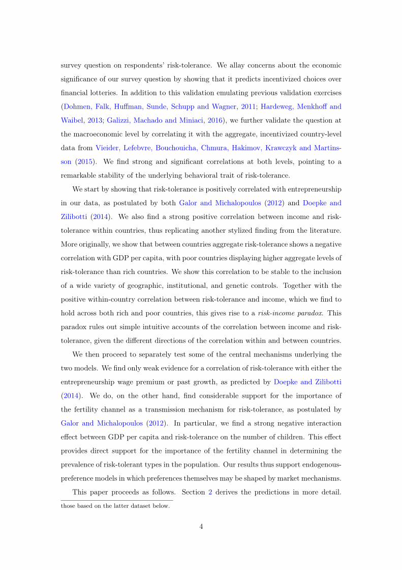
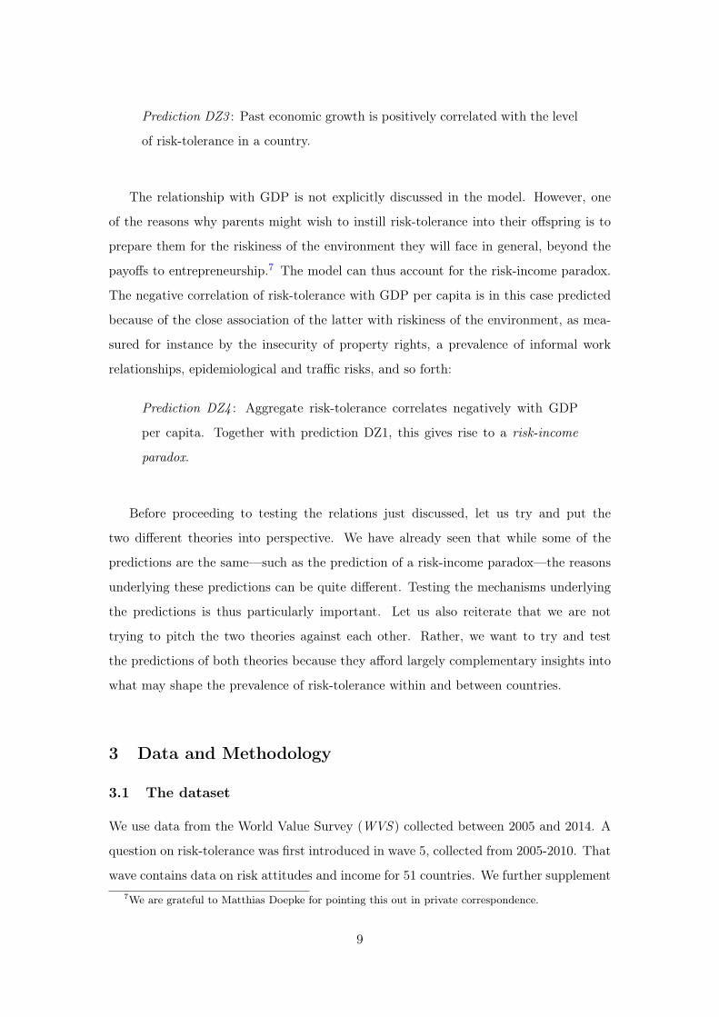
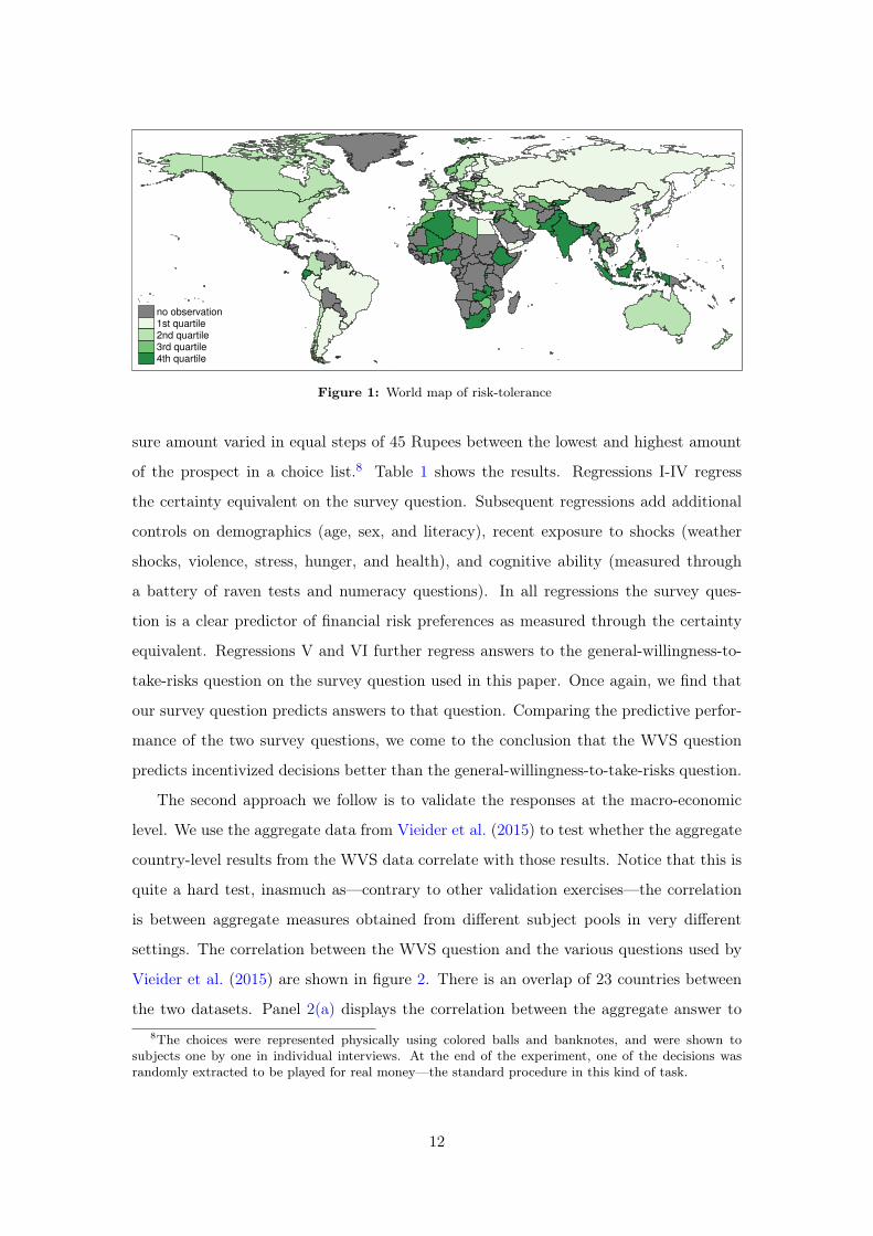
and shall simply refer to this measure as ‘risk-tolerance’. Figure 1 shows the countries
included in the dataset together with their level of risk-tolerance. The data cover a
total of 78 countries, and are representative within each country as well as providing
geographical and economic coverage of the whole world. Overall, the data cover 84% of
the world’s population, and 89% of its economic output.
Given the different formulation of this question relative to previously used survey
questions, it appears paramount to investigate whether it predicts risk preferences in the
sense usually intended by economists. To this end, we administered the survey question
together with an incentivised question to measure risk preferences to a sample repre-
sentative of the population of one district in Karnataka state, India. The incentivised
task consisted in eliciting the sure amount of money that is considered equally good
as a prospect giving a 50% probability of winning 450 Rupees or else nothing. The
11
no observation1st quartile2nd quartile3rd quartile4th quartile
Figure 1: World map of risk-tolerance
sure amount varied in equal steps of 45 Rupees between the lowest and highest amount
of the prospect in a choice list.8 Table 1 shows the results. Regressions I-IV regress
the certainty equivalent on the survey question. Subsequent regressions add additional
controls on demographics (age, sex, and literacy), recent exposure to shocks (weather
shocks, violence, stress, hunger, and health), and cognitive ability (measured through
a battery of raven tests and numeracy questions). In all regressions the survey ques-
tion is a clear predictor of financial risk preferences as measured through the certainty
equivalent. Regressions V and VI further regress answers to the general-willingness-to-
take-risks question on the survey question used in this paper. Once again, we find that
our survey question predicts answers to that question. Comparing the predictive perfor-
mance of the two survey questions, we come to the conclusion that the WVS question
predicts incentivized decisions better than the general-willingness-to-take-risks question.
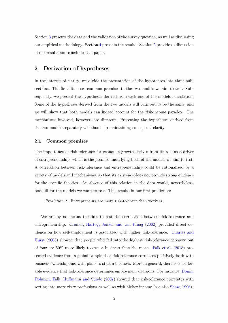
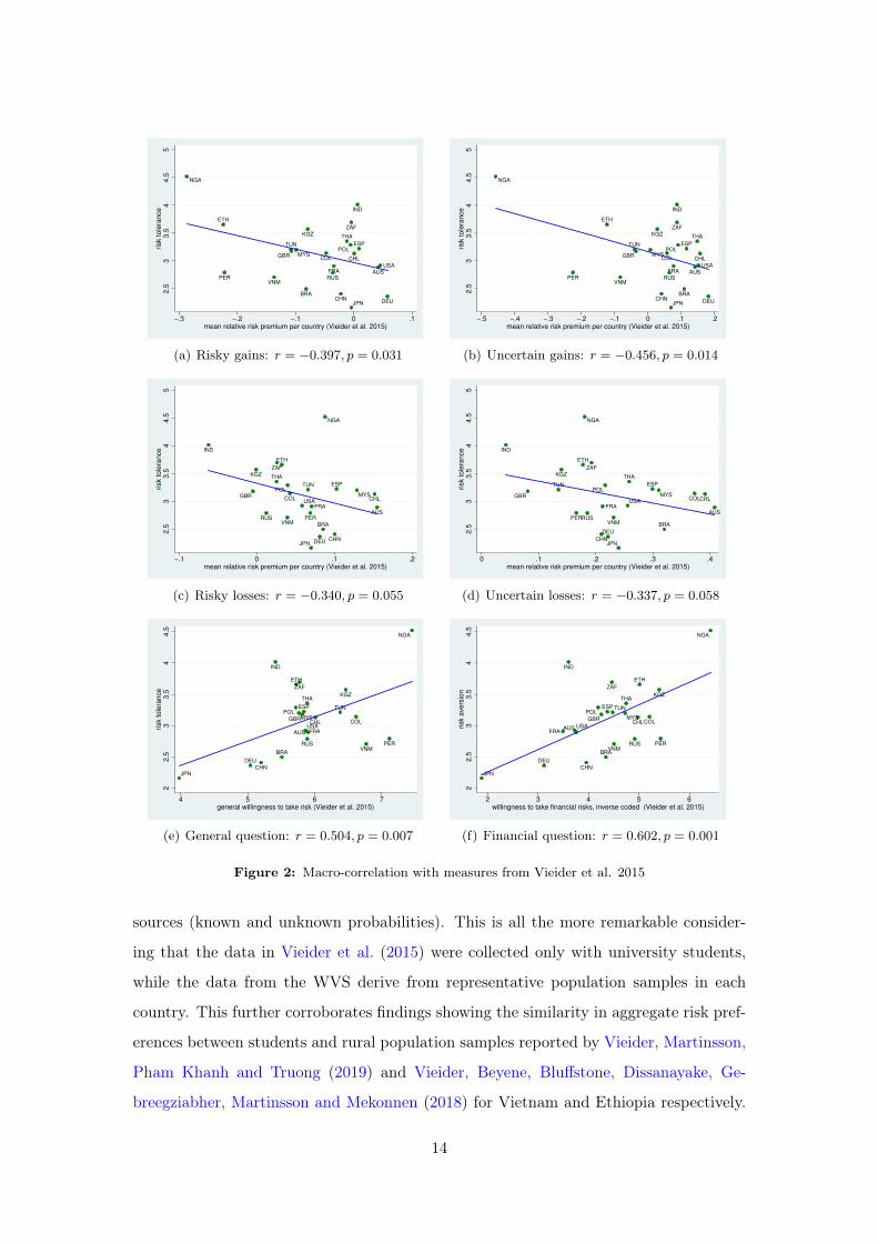
The second approach we follow is to validate the responses at the macro-economic
level. We use the aggregate data from Vieider et al. (2015) to test whether the aggregate
country-level results from the WVS data correlate with those results. Notice that this is
quite a hard test, inasmuch as—contrary to other validation exercises—the correlation
is between aggregate measures obtained from different subject pools in very different
settings. The correlation between the WVS question and the various questions used by
Vieider et al. (2015) are shown in figure 2. There is an overlap of 23 countries between
the two datasets. Panel 2(a) displays the correlation between the aggregate answer to8The choices were represented physically using colored balls and banknotes, and were shown to
subjects one by one in individual interviews. At the end of the experiment, one of the decisions wasrandomly extracted to be played for real money—the standard procedure in this kind of task.
12
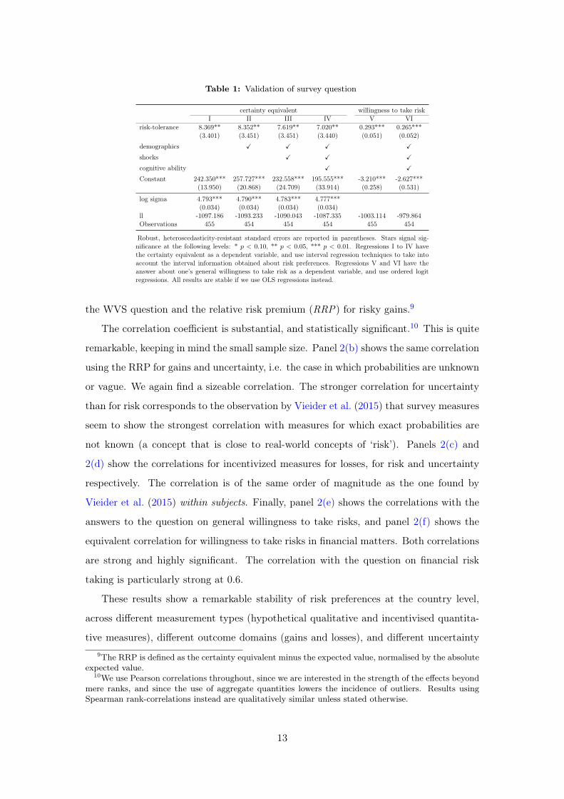
Table 1: Validation of survey question
certainty equivalent willingness to take riskI II III IV V VI
risk-tolerance 8.369** 8.352** 7.619** 7.020** 0.293*** 0.265***(3.401) (3.451) (3.451) (3.440) (0.051) (0.052)
demographics X X X X
shocks X X X
cognitive ability X X
Constant 242.350*** 257.727*** 232.558*** 195.555*** -3.210*** -2.627***(13.950) (20.868) (24.709) (33.914) (0.258) (0.531)
log sigma 4.793*** 4.790*** 4.783*** 4.777***(0.034) (0.034) (0.034) (0.034)
ll -1097.186 -1093.233 -1090.043 -1087.335 -1003.114 -979.864Observations 455 454 454 454 455 454
Robust, heteroscedasticity-resistant standard errors are reported in parentheses. Stars signal sig-nificance at the following levels: * p < 0.10, ** p < 0.05, *** p < 0.01. Regressions I to IV havethe certainty equivalent as a dependent variable, and use interval regression techniques to take intoaccount the interval information obtained about risk preferences. Regressions V and VI have theanswer about one’s general willingness to take risk as a dependent variable, and use ordered logitregressions. All results are stable if we use OLS regressions instead.
the WVS question and the relative risk premium (RRP) for risky gains.9
The correlation coefficient is substantial, and statistically significant.10 This is quite
remarkable, keeping in mind the small sample size. Panel 2(b) shows the same correlation
using the RRP for gains and uncertainty, i.e. the case in which probabilities are unknown
or vague. We again find a sizeable correlation. The stronger correlation for uncertainty
than for risk corresponds to the observation by Vieider et al. (2015) that survey measures
seem to show the strongest correlation with measures for which exact probabilities are
not known (a concept that is close to real-world concepts of ‘risk’). Panels 2(c) and
2(d) show the correlations for incentivized measures for losses, for risk and uncertainty
respectively. The correlation is of the same order of magnitude as the one found by
Vieider et al. (2015) within subjects. Finally, panel 2(e) shows the correlations with the
answers to the question on general willingness to take risks, and panel 2(f) shows the
equivalent correlation for willingness to take risks in financial matters. Both correlations
are strong and highly significant. The correlation with the question on financial risk
taking is particularly strong at 0.6.
These results show a remarkable stability of risk preferences at the country level,
across different measurement types (hypothetical qualitative and incentivised quantita-
tive measures), different outcome domains (gains and losses), and different uncertainty9The RRP is defined as the certainty equivalent minus the expected value, normalised by the absolute
expected value.10We use Pearson correlations throughout, since we are interested in the strength of the effects beyond
mere ranks, and since the use of aggregate quantities lowers the incidence of outliers. Results usingSpearman rank-correlations instead are qualitatively similar unless stated otherwise.
13
AUS
BRA
CHL
CHN
COL
ETH
FRA
DEU
IND
JPN
KGZ
MYS
NGA
PER
POL
RUSVNM
ZAF
ESP
THA
TUN
GBR
USA
2.5
33.5
44.5
5risk tole
rance
−.3 −.2 −.1 0 .1mean relative risk premium per country (Vieider et al. 2015)
(a) Risky gains: r = −0.397, p = 0.031
AUS
BRA
CHL
CHN
COL
ETH
FRA
DEU
IND
JPN
KGZ
MYS
NGA
PER
POL
RUSVNM
ZAF
ESP
THA
TUN
GBR
USA
2.5
33.5
44.5
5risk tole
rance
−.5 −.4 −.3 −.2 −.1 0 .1 .2mean relative risk premium per country (Vieider et al. 2015)
(b) Uncertain gains: r = −0.456, p = 0.014
AUS
BRA
CHL
CHN
COL
ETH
FRA
DEU
IND
JPN
KGZ
MYS
NGA
PER
POL
RUSVNM
ZAF
ESP
THA
TUN
GBRUSA
2.5
33.5
44.5
5risk tole
rance
−.1 0 .1 .2mean relative risk premium per country (Vieider et al. 2015)
(c) Risky losses: r = −0.340, p = 0.055
AUS
BRA
CHL
CHN
COL
ETH
FRA
DEU
IND
JPN
KGZ
MYS
NGA
PER
POL
RUSVNM
ZAF
ESP
THA
TUN
GBRUSA
2.5
33.5
44.5
5risk tole
rance
0 .1 .2 .3 .4mean relative risk premium per country (Vieider et al. 2015)
(d) Uncertain losses: r = −0.337, p = 0.058
AUS
BRA
CHL
CHN
COL
ETH
FRA
DEU
IND
JPN
KGZ
MYS
NGA
PER
POL
RUSVNM
ZAF
ESP
THA
TUN
GBR
USA
22.5
33.5
44.5
risk tole
rance
4 5 6 7general willingness to take risk (Vieider et al. 2015)
(e) General question: r = 0.504, p = 0.007
AUS
BRA
CHL
CHN
COL
ETH
FRA
DEU
IND
JPN
KGZ
MYS
NGA
PER
POL
RUSVNM
ZAF
ESP
THA
TUN
GBR
USA
22.5
33.5
44.5
risk a
vers
ion
2 3 4 5 6willingness to take financial risks, inverse coded (Vieider et al. 2015)
(f) Financial question: r = 0.602, p = 0.001
Figure 2: Macro-correlation with measures from Vieider et al. 2015
sources (known and unknown probabilities). This is all the more remarkable consider-
ing that the data in Vieider et al. (2015) were collected only with university students,
while the data from the WVS derive from representative population samples in each
country. This further corroborates findings showing the similarity in aggregate risk pref-
erences between students and rural population samples reported by Vieider, Martinsson,
Pham Khanh and Truong (2019) and Vieider, Beyene, Bluffstone, Dissanayake, Ge-
breegziabher, Martinsson and Mekonnen (2018) for Vietnam and Ethiopia respectively.
14
Similar conclusions were reached by Andersen, Harrison, Lau and Rutström (2010) for
Denmark and Fehr-Duda and Epper (2012) for Switzerland. Most importantly, however,
this validates the WVS measure of risk-tolerance as a proxy for financial risk aversion
measured in incentivized experiments.
3.3 Methodology
We use a hierarchical model to analyse the data. This method is specifically designed to
analyse data where several levels of analysis overlap, in which case OLS generally results
in biased estimates (Moulton, 1986). It provides standard errors corrected for the mul-
tilevel structure (Zeger, Liang and Albert, 1988), which makes them more conservative
than estimates obtained directly from individual-level regressions. Compared to estima-
tions using aggregate data, this approach avoids the so-called ecological fallacy, which
occurs when proportions of individual level characteristics are entered into aggregate
regressions (Robinson, 1950).
The hierarchical regression technique we use results in a generalization of linear
regression techniques whereby the residuals are not independent, but may be correlated
within higher level units (in our case, the different countries). We thus estimate a model
of the following form:
rij = Xijβ + uj + εij , (1)
where r indicates risk-tolerance, and the subscripts i and j indicate our two levels of
analysis—individuals and countries. The matrix X of observable characteristics may
contain indicators at the individual level or at the country level. This part of the estima-
tion takes the form of a standard OLS model. In multiple regression, the vector β will
consist of an intercept, β0, and a number of regression coefficients βk equal in number
to the number of independent variables.
4 Results
We present the results in several steps. We start by examining the role of risk-tolerance
as a determinant of entrepreneurship, and the microeconomic relationship between risk-
tolerance and income. We then present the risk-income paradox, juxtaposing the micro
15
and macro results directly. We subsequently continue our analysis with some tests of the
mechanisms postulated by the different models.
4.1 Microevidence on risk-tolerance, entrepreneurship, and income
We start by examining the evidence on the correlation of risk-tolerance with entrepreneur-
ship and with personal income at the microeconomic level. These correlations are closely
related from a conceptual point of view according to the model, which makes it natural
to present them together. We would also like to reiterate how these correlations cannot
be construed as definite tests of the theories, since such relationships can be conceptual-
ized based on a variety of different models. Nor is the evidence presented in this section
very novel, since both correlations have been discussed many times before. Nevertheless,
we deem it desirable to test them in our data, both because these correlations are at
times still contested by some scholars11, and because their absence would bode ill for our
enterprise of testing some of the more original predictions of the two models.
We start from the correlation between risk-tolerance and entrepreneurship. We use a
question in the WVS where people declare whether they are self-employed, work for the
government, private firms, or in the nongovernmental sector. Table 2 shows a number of
regressions of a dummy variable indicating self-employment on risk-tolerance. Regression
I establishes the basic relationship—risk-tolerance shows a clear and highly significant
positive correlation with entrepreneurship. Regression II adds a number of individual-
level variables, including age and gender, as well as controls of educational attainment
and marital status. The correlation between risk-tolerance and self-employment remains
stable, and results even somewhat reinforced.
Regression III adds personal income to the regression. This control is essential in
order to ensure that the correlation is not spurious, and purely driven by the higher
income earned by entrepreneurs in most countries. This assumes that risk-tolerance and
income are themselves rather strongly correlated—an issue that we will examine shortly.
Risk-tolerance remains a strong predictor of entrepreneurship even after controlling for11We included a brief literature review of the correlation of risk-tolerance and entrepreneurship above.
In terms of the correlation between risk-tolerance and income, many studies have found a positiverelationship between risk-tolerance and income (Dohmen et al., 2011; Gloede, Menkhoff and Waibel,2015; Hopland, Matsen and Strøm, 2016; Vieider et al., 2018; Falk et al., 2018), several others havefound no correlation (Binswanger, 1980; Cardenas and Carpenter, 2013; Noussair, Trautmann and van deKuilen, 2014), while others still have observed mixed results (Booij, Praag and van de Kuilen, 2010;Tanaka, Camerer and Nguyen, 2010; von Gaudecker, van Soest and Wengström, 2011). See Hopland etal. (2016) for a more in-depth review.
16
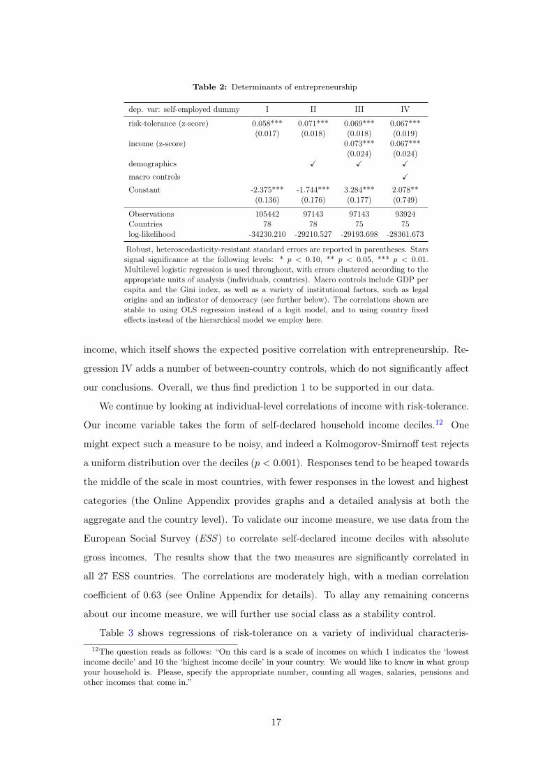
Table 2: Determinants of entrepreneurship
dep. var: self-employed dummy I II III IV
risk-tolerance (z-score) 0.058*** 0.071*** 0.069*** 0.067***(0.017) (0.018) (0.018) (0.019)
income (z-score) 0.073*** 0.067***(0.024) (0.024)
demographics X X X
macro controls X
Constant -2.375*** -1.744*** 3.284*** 2.078**(0.136) (0.176) (0.177) (0.749)
Observations 105442 97143 97143 93924Countries 78 78 75 75log-likelihood -34230.210 -29210.527 -29193.698 -28361.673
Robust, heteroscedasticity-resistant standard errors are reported in parentheses. Starssignal significance at the following levels: * p < 0.10, ** p < 0.05, *** p < 0.01.Multilevel logistic regression is used throughout, with errors clustered according to theappropriate units of analysis (individuals, countries). Macro controls include GDP percapita and the Gini index, as well as a variety of institutional factors, such as legalorigins and an indicator of democracy (see further below). The correlations shown arestable to using OLS regression instead of a logit model, and to using country fixedeffects instead of the hierarchical model we employ here.
income, which itself shows the expected positive correlation with entrepreneurship. Re-
gression IV adds a number of between-country controls, which do not significantly affect
our conclusions. Overall, we thus find prediction 1 to be supported in our data.
We continue by looking at individual-level correlations of income with risk-tolerance.
Our income variable takes the form of self-declared household income deciles.12 One
might expect such a measure to be noisy, and indeed a Kolmogorov-Smirnoff test rejects
a uniform distribution over the deciles (p < 0.001). Responses tend to be heaped towards
the middle of the scale in most countries, with fewer responses in the lowest and highest
categories (the Online Appendix provides graphs and a detailed analysis at both the
aggregate and the country level). To validate our income measure, we use data from the
European Social Survey (ESS ) to correlate self-declared income deciles with absolute
gross incomes. The results show that the two measures are significantly correlated in
all 27 ESS countries. The correlations are moderately high, with a median correlation
coefficient of 0.63 (see Online Appendix for details). To allay any remaining concerns
about our income measure, we will further use social class as a stability control.
Table 3 shows regressions of risk-tolerance on a variety of individual characteris-12The question reads as follows: “On this card is a scale of incomes on which 1 indicates the ‘lowest
income decile’ and 10 the ‘highest income decile’ in your country. We would like to know in what groupyour household is. Please, specify the appropriate number, counting all wages, salaries, pensions andother incomes that come in.”
17
tics.13 Regression I uses income as the sole explanatory variable, and shows a clear
positive correlation between risk-tolerance and income. Regression II adds a number of
demographic controls. The income coefficient drops somewhat as a result of this, but
nonetheless remains highly significant. The higher the level of education, the more risk-
tolerant respondents are. There are two possible explanations for this. A straightforward
explanation might be that risk-tolerance is positively correlated with cognitive ability
(Dohmen, Falk, Huffman and Sunde, 2010; Benjamin, Brown and Shapiro, 2013), and
that education serves as a proxy for cognitive ability. However, a recent investigation
by Andersson, Tyran, Wengström and Holm (2016) cast doubt on the stability of the
correlation between risk aversion and cognitive ability. An alternative explanation may
then be that education proxies for income, given that measures of the latter are coarse
and the two are typically highly correlated.14
We find females to be significantly less risk-tolerant than males. This corresponds
to standard findings in the literature (Croson and Gneezy, 2009), even though there
may exist differences according to the measurement method employed (di Falco and
Vieider, 2018). As expected, we find risk-tolerance to decrease in age. Risk-tolerance
also strongly increases in age squared, however. In terms of marital status, every category
except widowers are more risk-tolerant than the reference category of married people.
This could be driven by people becoming less risk-tolerant when they marry (Görlitz and
Tamm, 2015), but it may just as well result from less risk-tolerant people getting married
more frequently or sooner in life, and then staying married with a higher likelihood
(Schmidt, 2008).
Regression III further adds self-declared health state, encoded from 1 (very good) to
5 (very poor). Risk-tolerance decreases in this variable, indicating that people in poor
health tend to be less risk-tolerant. Regression IV introduces a variable measuring life13While the models we test predict causality to run from risk-tolerance to income passing through
the entrepreneurship decision, in reality the causality in the risk-income relationship could run in eitherdirection, and may well constitute a self-reinforcing feedback cycle. Indeed, the clear causal directionemerges from the model due to the abstraction from intergenerational transmission of wealth and skills,in addition to preferences. While most of the literature in labor economics emphasizes the causalityfrom risk-tolerance to income passing through job choice ( e g. Bonin et al., 2007), the literature indevelopment economics generally emphasizes the opposite direction of causality (see Haushofer and Fehr,2014, for a review). Making risk-tolerance the dependent variable allows us to examine the correlates ofrisk-tolerance, which is the truly novel measure at the center of our analysis. The correlation betweenincome and risk-tolerance is unaffected if we take income as the dependent variable instead—a regressionwith income as the dependent variable is shown in the Online Appendix.
14Our data indeed show a substantial correlation between income decile and education. In particular,each higher level of education results in a significantly higher response on the income decile scale—seeonline appendix for the regression result.
18
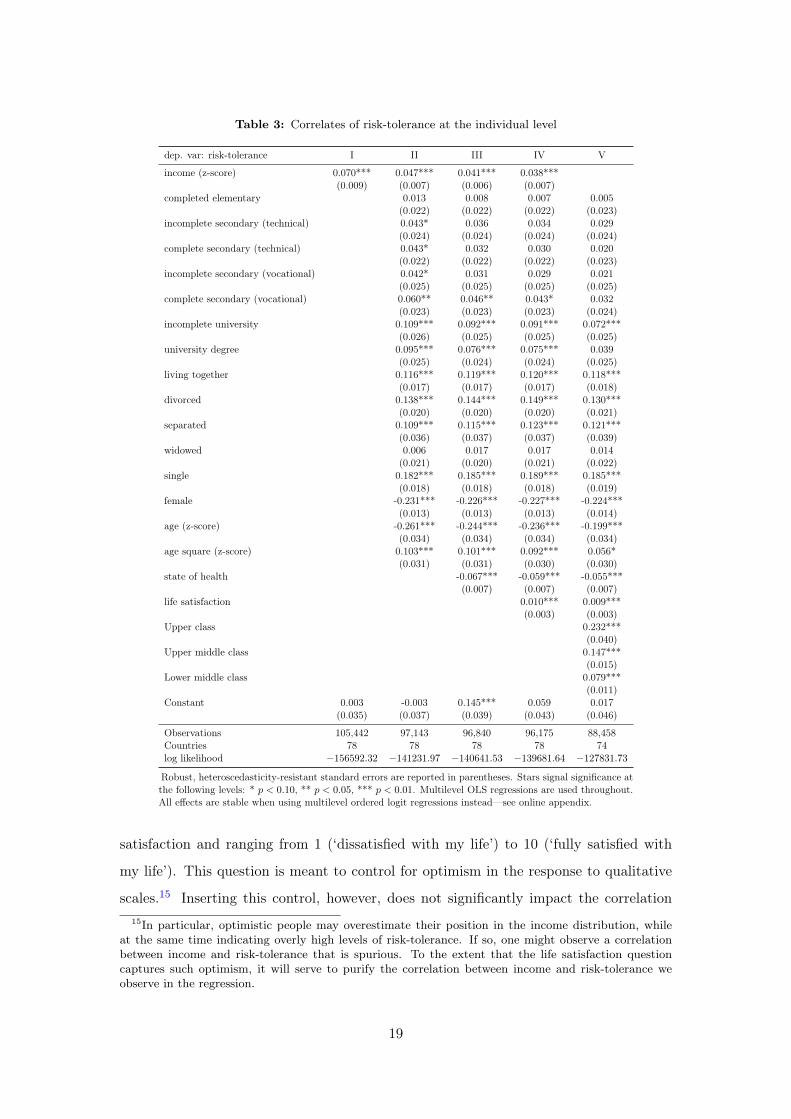
Table 3: Correlates of risk-tolerance at the individual level
dep. var: risk-tolerance I II III IV V
income (z-score) 0.070*** 0.047*** 0.041*** 0.038***(0.009) (0.007) (0.006) (0.007)
completed elementary 0.013 0.008 0.007 0.005(0.022) (0.022) (0.022) (0.023)
incomplete secondary (technical) 0.043* 0.036 0.034 0.029(0.024) (0.024) (0.024) (0.024)
complete secondary (technical) 0.043* 0.032 0.030 0.020(0.022) (0.022) (0.022) (0.023)
incomplete secondary (vocational) 0.042* 0.031 0.029 0.021(0.025) (0.025) (0.025) (0.025)
complete secondary (vocational) 0.060** 0.046** 0.043* 0.032(0.023) (0.023) (0.023) (0.024)
incomplete university 0.109*** 0.092*** 0.091*** 0.072***(0.026) (0.025) (0.025) (0.025)
university degree 0.095*** 0.076*** 0.075*** 0.039(0.025) (0.024) (0.024) (0.025)
living together 0.116*** 0.119*** 0.120*** 0.118***(0.017) (0.017) (0.017) (0.018)
divorced 0.138*** 0.144*** 0.149*** 0.130***(0.020) (0.020) (0.020) (0.021)
separated 0.109*** 0.115*** 0.123*** 0.121***(0.036) (0.037) (0.037) (0.039)
widowed 0.006 0.017 0.017 0.014(0.021) (0.020) (0.021) (0.022)
single 0.182*** 0.185*** 0.189*** 0.185***(0.018) (0.018) (0.018) (0.019)
female -0.231*** -0.226*** -0.227*** -0.224***(0.013) (0.013) (0.013) (0.014)
age (z-score) -0.261*** -0.244*** -0.236*** -0.199***(0.034) (0.034) (0.034) (0.034)
age square (z-score) 0.103*** 0.101*** 0.092*** 0.056*(0.031) (0.031) (0.030) (0.030)
state of health -0.067*** -0.059*** -0.055***(0.007) (0.007) (0.007)
life satisfaction 0.010*** 0.009***(0.003) (0.003)
Upper class 0.232***(0.040)
Upper middle class 0.147***(0.015)
Lower middle class 0.079***(0.011)
Constant 0.003 -0.003 0.145*** 0.059 0.017(0.035) (0.037) (0.039) (0.043) (0.046)
Observations 105,442 97,143 96,840 96,175 88,458Countries 78 78 78 78 74log likelihood −156592.32 −141231.97 −140641.53 −139681.64 −127831.73
Robust, heteroscedasticity-resistant standard errors are reported in parentheses. Stars signal significance atthe following levels: * p < 0.10, ** p < 0.05, *** p < 0.01. Multilevel OLS regressions are used throughout.All effects are stable when using multilevel ordered logit regressions instead—see online appendix.
satisfaction and ranging from 1 (‘dissatisfied with my life’) to 10 (‘fully satisfied with
my life’). This question is meant to control for optimism in the response to qualitative
scales.15 Inserting this control, however, does not significantly impact the correlation15In particular, optimistic people may overestimate their position in the income distribution, while
at the same time indicating overly high levels of risk-tolerance. If so, one might observe a correlationbetween income and risk-tolerance that is spurious. To the extent that the life satisfaction questioncaptures such optimism, it will serve to purify the correlation between income and risk-tolerance weobserve in the regression.
19
between risk-tolerance and income.
Finally, regression V provides a stability test by investigating social class as a substi-
tute for the income measure. We enter three separate dummies for whether a respondent
belongs to the ‘upper class’, the ‘upper middle class’, or the ‘lower middle class’, which
are measured relative to ‘working class’ and ‘lower class’. We lump the latter two to-
gether in the analysis since in some countries very few respondents have indicated to
belong to the ‘lower class’. All three dummy variables show the expected positive effect,
indicating higher levels of risk-tolerance for higher classes. The effect can be seen to be
larger the higher the class, so that respondents belonging to the upper middle class are
not only more risk-tolerant than respondents from the working and lower classes, but
also than respondents from the lower middle class. Equivalently, respondents from the
upper class are more risk-tolerant than respondents from any of the middle classes, as
well as the lower classes.
4.2 A risk-income paradox
We now move on to juxtaposing the effects of personal income with those of GDP per
capita in one and the same regression. Presenting empirical evidence on the paradox
constitutes an original contribution of our paper. Other than the results presented above,
the paradox also constitutes an original prediction of the two models, which is a priori
far from obvious, and can thus serve as a first test of their validity. It is interesting that
both models predict this paradox, although based on different reasons (see discussions
above surrounding predictions GM1 and GM2, and DZ1 and DZ4 for the details).
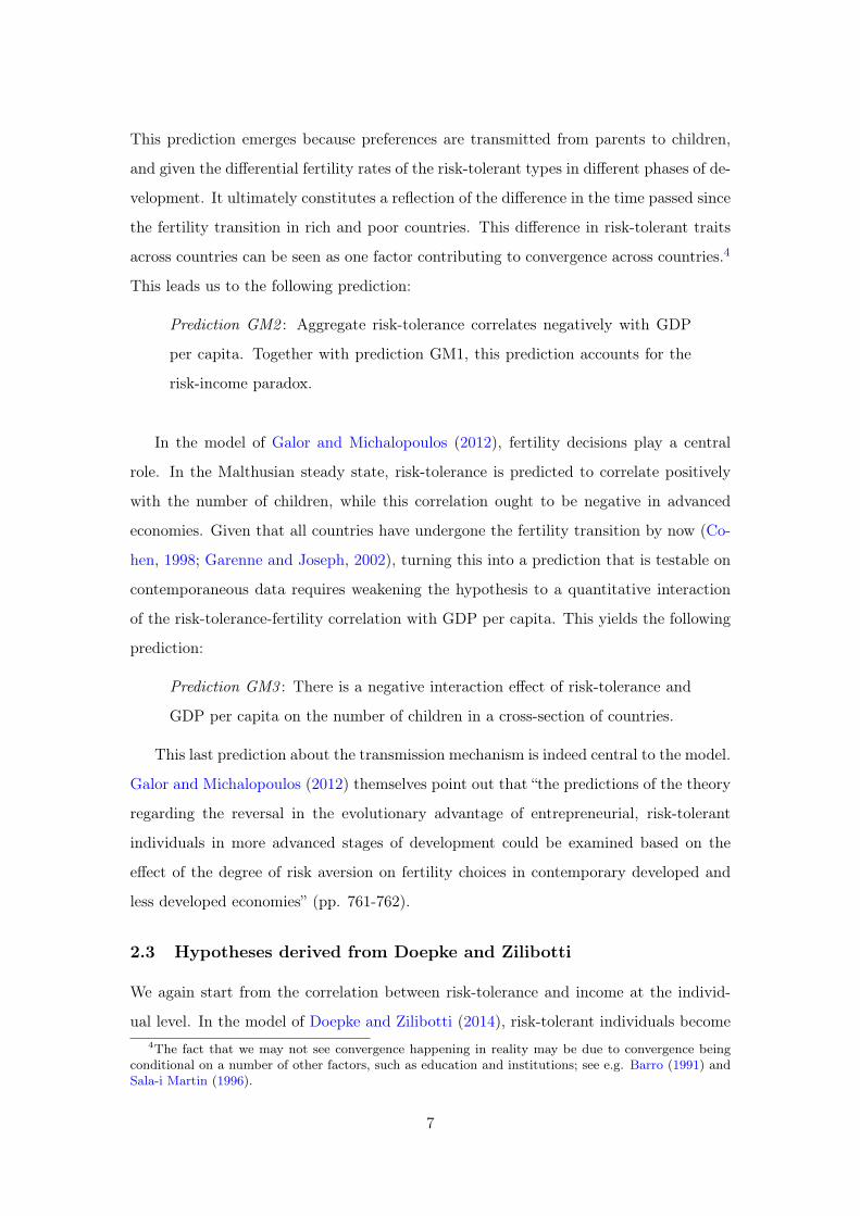
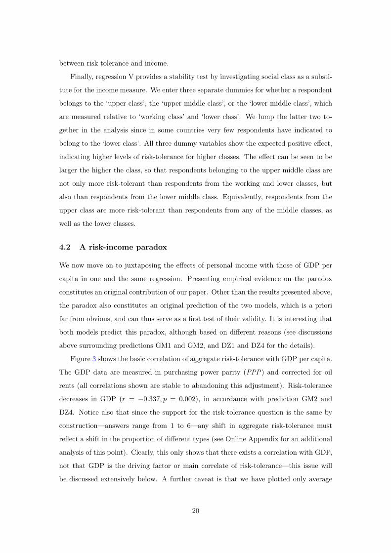
Figure 3 shows the basic correlation of aggregate risk-tolerance with GDP per capita.
The GDP data are measured in purchasing power parity (PPP) and corrected for oil
rents (all correlations shown are stable to abandoning this adjustment). Risk-tolerance
decreases in GDP (r = −0.337, p = 0.002), in accordance with prediction GM2 and
DZ4. Notice also that since the support for the risk-tolerance question is the same by
construction—answers range from 1 to 6—any shift in aggregate risk-tolerance must
reflect a shift in the proportion of different types (see Online Appendix for an additional
analysis of this point). Clearly, this only shows that there exists a correlation with GDP,
not that GDP is the driving factor or main correlate of risk-tolerance—this issue will
be discussed extensively below. A further caveat is that we have plotted only average
20
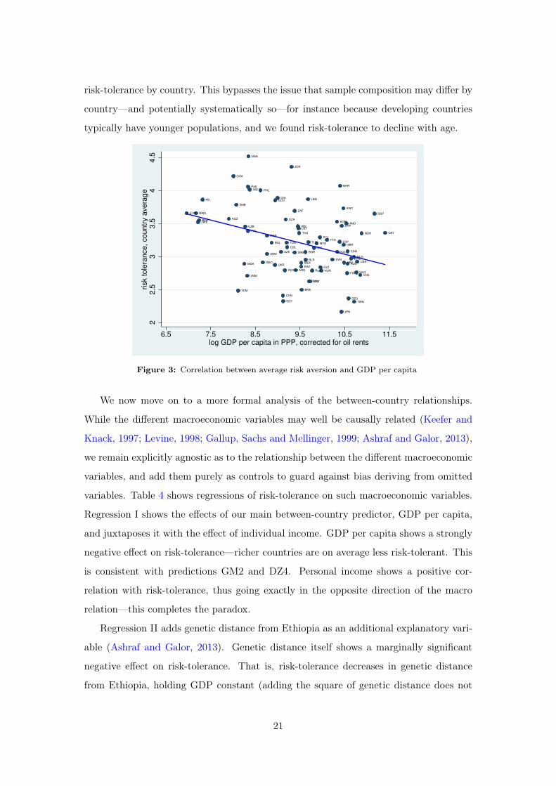
risk-tolerance by country. This bypasses the issue that sample composition may differ by
country—and potentially systematically so—for instance because developing countries
typically have younger populations, and we found risk-tolerance to decline with age.
ROU
BHR
DZA
TTO
MAR
HKGARG
KWT
QATNOR
KGZ
IRN
MDA
CHE
ARM
RWA
KAZ
AZE
TWN
AUS
LBY
AND
UKR
IDN LBN
NZL
GEO MEX
PAL
EST
JOR
ETH
THA
YEM
MYS
PER
SGP
TUN
ZAF
SWE
URY
KOR
BLRUSA
TUR
CYP
ECU
BGR
COL
VNM
PHL
IRQ
CAN
POL
DEU
SRB
CHL
UZB
SVN
ZWE
HUN
ESP
FIN
CHN
PAKIND
JPN
NGA
BRA
EGY
ZMB
GHA
FRA
GBR
BFA
MLI
RUS
NLD
22.5
33.5
44.5
risk tole
rance, countr
y a
vera
ge
6.5 7.5 8.5 9.5 10.5 11.5log GDP per capita in PPP, corrected for oil rents
Figure 3: Correlation between average risk aversion and GDP per capita
We now move on to a more formal analysis of the between-country relationships.
While the different macroeconomic variables may well be causally related (Keefer and
Knack, 1997; Levine, 1998; Gallup, Sachs and Mellinger, 1999; Ashraf and Galor, 2013),
we remain explicitly agnostic as to the relationship between the different macroeconomic
variables, and add them purely as controls to guard against bias deriving from omitted
variables. Table 4 shows regressions of risk-tolerance on such macroeconomic variables.
Regression I shows the effects of our main between-country predictor, GDP per capita,
and juxtaposes it with the effect of individual income. GDP per capita shows a strongly
negative effect on risk-tolerance—richer countries are on average less risk-tolerant. This
is consistent with predictions GM2 and DZ4. Personal income shows a positive cor-
relation with risk-tolerance, thus going exactly in the opposite direction of the macro
relation—this completes the paradox.
Regression II adds genetic distance from Ethiopia as an additional explanatory vari-
able (Ashraf and Galor, 2013). Genetic distance itself shows a marginally significant
negative effect on risk-tolerance. That is, risk-tolerance decreases in genetic distance
from Ethiopia, holding GDP constant (adding the square of genetic distance does not
21
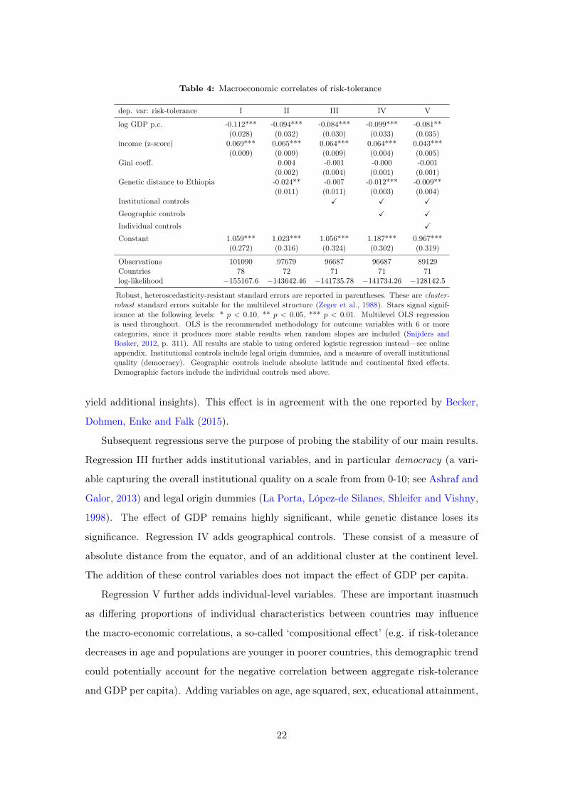
Table 4: Macroeconomic correlates of risk-tolerance
dep. var: risk-tolerance I II III IV V
log GDP p.c. -0.112*** -0.094*** -0.084*** -0.099*** -0.081**(0.028) (0.032) (0.030) (0.033) (0.035)
income (z-score) 0.069*** 0.065*** 0.064*** 0.064*** 0.043***(0.009) (0.009) (0.009) (0.004) (0.005)
Gini coeff. 0.004 -0.001 -0.000 -0.001(0.002) (0.004) (0.001) (0.001)
Genetic distance to Ethiopia -0.024** -0.007 -0.012*** -0.009**(0.011) (0.011) (0.003) (0.004)
Institutional controls X X X
Geographic controls X X
Individual controls X
Constant 1.059*** 1.023*** 1.056*** 1.187*** 0.967***(0.272) (0.316) (0.324) (0.302) (0.319)
Observations 101090 97679 96687 96687 89129Countries 78 72 71 71 71log-likelihood −155167.6 −143642.46 −141735.78 −141734.26 −128142.5
Robust, heteroscedasticity-resistant standard errors are reported in parentheses. These are cluster-robust standard errors suitable for the multilevel structure (Zeger et al., 1988). Stars signal signif-icance at the following levels: * p < 0.10, ** p < 0.05, *** p < 0.01. Multilevel OLS regressionis used throughout. OLS is the recommended methodology for outcome variables with 6 or morecategories, since it produces more stable results when random slopes are included (Snijders andBosker, 2012, p. 311). All results are stable to using ordered logistic regression instead—see onlineappendix. Institutional controls include legal origin dummies, and a measure of overall institutionalquality (democracy). Geographic controls include absolute latitude and continental fixed effects.Demographic factors include the individual controls used above.
yield additional insights). This effect is in agreement with the one reported by Becker,
Dohmen, Enke and Falk (2015).
Subsequent regressions serve the purpose of probing the stability of our main results.
Regression III further adds institutional variables, and in particular democracy (a vari-
able capturing the overall institutional quality on a scale from from 0-10; see Ashraf and
Galor, 2013) and legal origin dummies (La Porta, López-de Silanes, Shleifer and Vishny,
1998). The effect of GDP remains highly significant, while genetic distance loses its
significance. Regression IV adds geographical controls. These consist of a measure of
absolute distance from the equator, and of an additional cluster at the continent level.
The addition of these control variables does not impact the effect of GDP per capita.
Regression V further adds individual-level variables. These are important inasmuch
as differing proportions of individual characteristics between countries may influence
the macro-economic correlations, a so-called ‘compositional effect’ (e.g. if risk-tolerance
decreases in age and populations are younger in poorer countries, this demographic trend
could potentially account for the negative correlation between aggregate risk-tolerance
and GDP per capita). Adding variables on age, age squared, sex, educational attainment,
22
marital status, and relative personal income does not affect our conclusion in any way.
The effect of income can be seen to go in the opposite direction of the one of GDP
per capita, thus directly visualizing the risk-income paradox. Overall, this shows that
the effect of GDP per capita is stable to a variety of the most common macroeconomic
correlates of GDP.
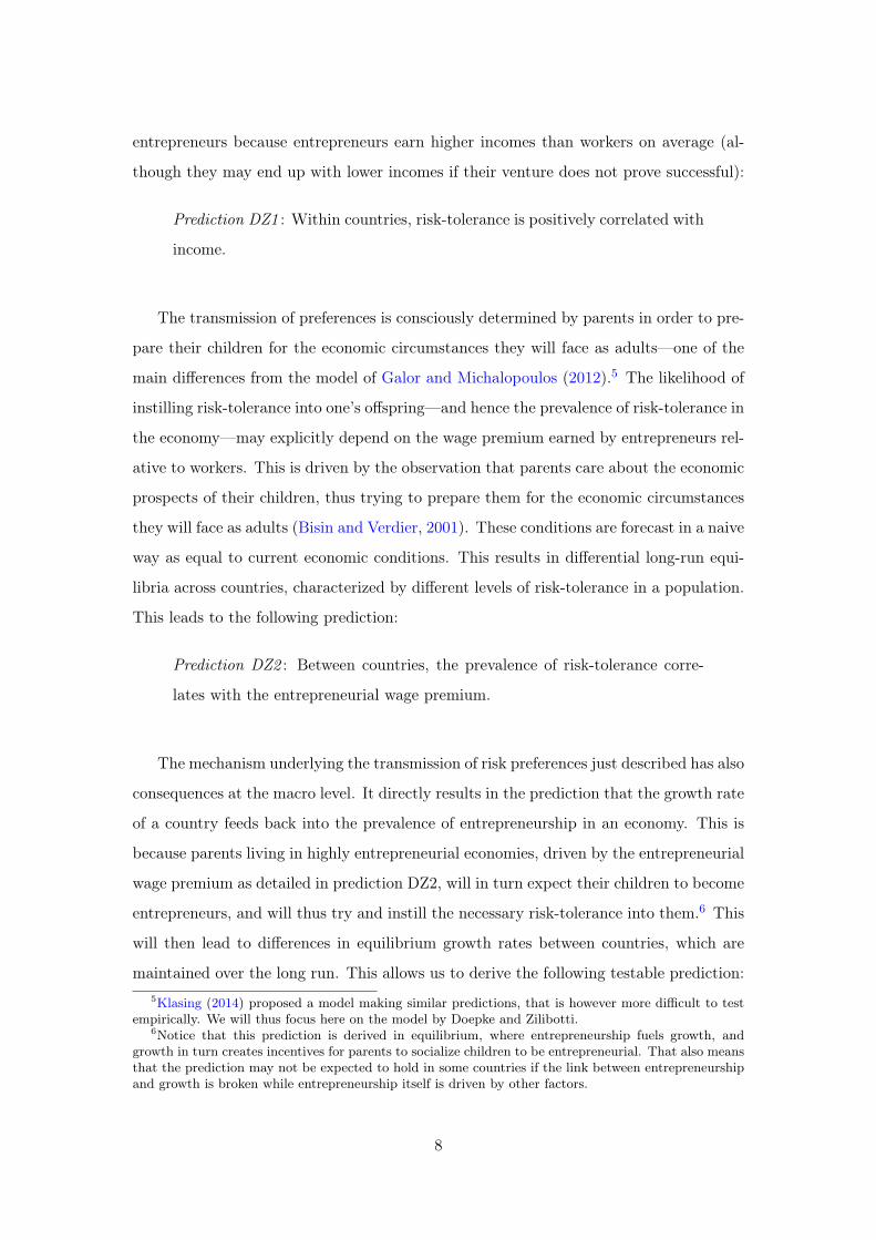
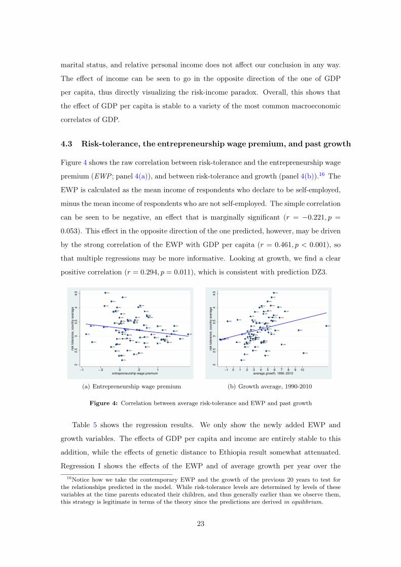
4.3 Risk-tolerance, the entrepreneurship wage premium, and past growth
Figure 4 shows the raw correlation between risk-tolerance and the entrepreneurship wage
premium (EWP ; panel 4(a)), and between risk-tolerance and growth (panel 4(b)).16 The
EWP is calculated as the mean income of respondents who declare to be self-employed,
minus the mean income of respondents who are not self-employed. The simple correlation
can be seen to be negative, an effect that is marginally significant (r = −0.221, p =
0.053). This effect in the opposite direction of the one predicted, however, may be driven
by the strong correlation of the EWP with GDP per capita (r = 0.461, p < 0.001), so
that multiple regressions may be more informative. Looking at growth, we find a clear
positive correlation (r = 0.294, p = 0.011), which is consistent with prediction DZ3.
DZA
BHR
ROU
MDAUKRAUS
TWN
QAT
HKG
TTO
ARM
NOR
KAZ
MAR
KGZ
LBY
CHE
AND
AZE
IRN
IDN
KWT
RWA
EST
KOR
TUNMYS
SWE
MEX
PER
GEO
SGP
BLR
ZAF
CYP
NZL
PAL
URY
TUR
JOR
ETH
ECU
THA
LBN
USA
YEM
POL
CHL
BGR
DEU
CAN
HUN
SRB
ESP
CHN
PHL
COL
FIN
IRQ
UZB
VNM
PAK
SVN
ZWE
ZMB
GHA
NGA
JPN
BRA
IND
EGY
RUS
FRA
MLI
GBR
BFA
NLD
22.5
33.5
44.5
risk tole
rance, countr
y a
vera
ge
−1 −.5 0 .5 1entrepreneurship wage premium
(a) Entrepreneurship wage premium
DZA
BHR
ROU
MDAUKR AUS
QAT
HKG
TTO
ARM
NOR
KAZ
MAR
KGZ
ARG
LBY
CHE
AND
AZE
IRN
IDN
KWT
RWA
EST
KOR
TUN MYS
SWE
MEX
PER
GEO
SGP
BLR
ZAF
CYP
NZL
URY
TUR
JOR
ETH
ECU
THA
LBN
USA
YEM
POL
CHL
BGR
DEU
CAN
HUN
ESP
CHN
PHL
COL
FIN
IRQ
UZB
VNM
PAK
SVN
ZWE
ZMB
GHA
NGA
JPN
BRA
IND
EGY
RUS
FRA
MLI
GBR
BFA
NLD
22.5
33.5
44.5
risk tole
rance, countr
y a
vera
ge
−1 0 1 2 3 4 5 6 7 8 9 10average growth, 1990−2010
(b) Growth average, 1990-2010
Figure 4: Correlation between average risk-tolerance and EWP and past growth
Table 5 shows the regression results. We only show the newly added EWP and
growth variables. The effects of GDP per capita and income are entirely stable to this
addition, while the effects of genetic distance to Ethiopia result somewhat attenuated.
Regression I shows the effects of the EWP and of average growth per year over the16Notice how we take the contemporary EWP and the growth of the previous 20 years to test for
the relationships predicted in the model. While risk-tolerance levels are determined by levels of thesevariables at the time parents educated their children, and thus generally earlier than we observe them,this strategy is legitimate in terms of the theory since the predictions are derived in equilibrium.
23
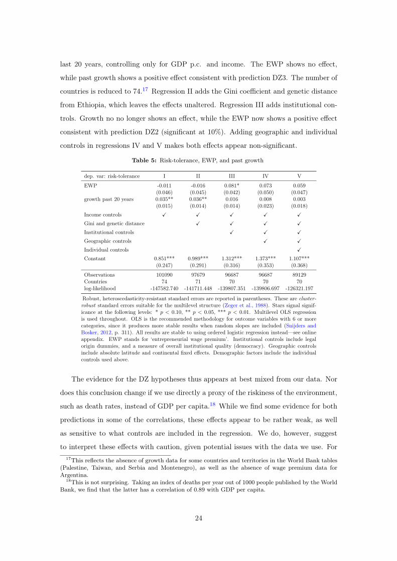
last 20 years, controlling only for GDP p.c. and income. The EWP shows no effect,
while past growth shows a positive effect consistent with prediction DZ3. The number of
countries is reduced to 74.17 Regression II adds the Gini coefficient and genetic distance
from Ethiopia, which leaves the effects unaltered. Regression III adds institutional con-
trols. Growth no no longer shows an effect, while the EWP now shows a positive effect
consistent with prediction DZ2 (significant at 10%). Adding geographic and individual
controls in regressions IV and V makes both effects appear non-significant.
Table 5: Risk-tolerance, EWP, and past growth
dep. var: risk-tolerance I II III IV V
EWP -0.011 -0.016 0.081* 0.073 0.059(0.046) (0.045) (0.042) (0.050) (0.047)
growth past 20 years 0.035** 0.036** 0.016 0.008 0.003(0.015) (0.014) (0.014) (0.023) (0.018)
Income controls X X X X X
Gini and genetic distance X X X X
Institutional controls X X X
Geographic controls X X
Individual controls X
Constant 0.851*** 0.989*** 1.312*** 1.373*** 1.107***(0.247) (0.291) (0.316) (0.353) (0.368)
Observations 101090 97679 96687 96687 89129Countries 74 71 70 70 70log-likelihood -147582.740 -141711.448 -139807.351 -139806.697 -126321.197
Robust, heteroscedasticity-resistant standard errors are reported in parentheses. These are cluster-robust standard errors suitable for the multilevel structure (Zeger et al., 1988). Stars signal signif-icance at the following levels: * p < 0.10, ** p < 0.05, *** p < 0.01. Multilevel OLS regressionis used throughout. OLS is the recommended methodology for outcome variables with 6 or morecategories, since it produces more stable results when random slopes are included (Snijders andBosker, 2012, p. 311). All results are stable to using ordered logistic regression instead—see onlineappendix. EWP stands for ‘entrepreneurial wage premium’. Institutional controls include legalorigin dummies, and a measure of overall institutional quality (democracy). Geographic controlsinclude absolute latitude and continental fixed effects. Demographic factors include the individualcontrols used above.
The evidence for the DZ hypotheses thus appears at best mixed from our data. Nor
does this conclusion change if we use directly a proxy of the riskiness of the environment,
such as death rates, instead of GDP per capita.18 While we find some evidence for both
predictions in some of the correlations, these effects appear to be rather weak, as well
as sensitive to what controls are included in the regression. We do, however, suggest
to interpret these effects with caution, given potential issues with the data we use. For17This reflects the absence of growth data for some countries and territories in the World Bank tables
(Palestine, Taiwan, and Serbia and Montenegro), as well as the absence of wage premium data forArgentina.
18This is not surprising. Taking an index of deaths per year out of 1000 people published by the WorldBank, we find that the latter has a correlation of 0.89 with GDP per capita.
24
instance, the entrepreneurial wage premium may be a rather noisy measure, since what
constitutes ‘entrepreneurship’ may be interpreted very differently across countries. It is
furthermore unclear whether he particular measure of riskiness of the environment given
by death rates is the correct one to use as a control. Future research will have to probe
these points in more depth.
4.4 Risk-tolerance and fertility
A specific prediction emerging from the model by Galor and Michalopoulos (2012) that is
not shared with the models of Doepke and Zilibotti (2014) is prediction GM3—the depen-
dence of the correlation between risk-tolerance and fertility on the level of development.
In particular, the prediction is that risk-tolerance will be strongly negatively correlated
with number of children in developed countries, while this correlation is expected to
be positive in countries that find themselves in a Malthusian equilibrium. Arguably,
however, no country nowadays can be described as finding itself in a Malthusian steady
state. Indeed, it has been argued that virtually all African countries had started the
fertility transition by the late 1980s (Cohen, 1998). Using more reliable data, Garenne
and Joseph (2002) dated the incept of the fertility transition even earlier, showing that
the fertility transition had started in most sub-Saharan African countries by the mid
1970s at least in the cities, with the countryside typically lagging behind by a decade or
more. This leads to a weaker prediction of a negative interaction effect of risk-tolerance
and GDP per capita on the number of children.
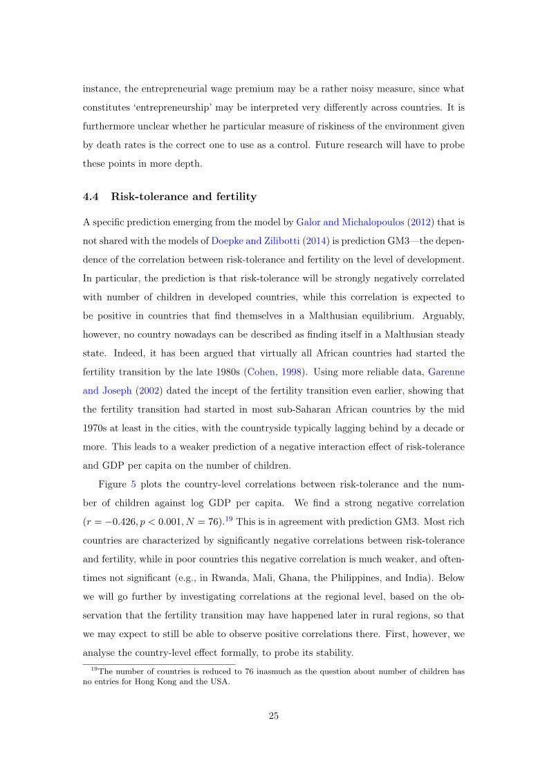
Figure 5 plots the country-level correlations between risk-tolerance and the num-
ber of children against log GDP per capita. We find a strong negative correlation
(r = −0.426, p < 0.001, N = 76).19 This is in agreement with prediction GM3. Most rich
countries are characterized by significantly negative correlations between risk-tolerance
and fertility, while in poor countries this negative correlation is much weaker, and often-
times not significant (e.g., in Rwanda, Mali, Ghana, the Philippines, and India). Below
we will go further by investigating correlations at the regional level, based on the ob-
servation that the fertility transition may have happened later in rural regions, so that
we may expect to still be able to observe positive correlations there. First, however, we
analyse the country-level effect formally, to probe its stability.19The number of countries is reduced to 76 inasmuch as the question about number of children has
no entries for Hong Kong and the USA.
25
DZA
AND
AZE
ARG
AUS
BHR
ARM
BRABGR
BLR
CAN
CHL
CHN
TWN
COL
CYP
ECU
ETH
EST
FIN
FRA
GEO
PAL
DEU
GHA
HUN
IND
IDN
IRN
IRQ
JPN
KAZ
JOR KOR
KWT
KGZ
LBN
LBY
MYS
MLI
MEXMDA
MAR
NLD
NZL
NGA
NOR
PAK
PER
PHL
POL
QAT
ROURUS
RWA
SGP
VNM
SVN
ZAF
ZWE
ESP
SWE
CHE
THA
TTO
TUN
TURUKR
EGY
GBR
BFA
URY
UZB
YEM
SRB
ZMB
−.4
−.3
−.2
−.1
0risk t
ole
ran
ce
−ch
ildre
n c
orr
ela
tio
n
7 9 11log GDP p.c.
fitted line
Figure 5: risk-tolerance-children correlation by GDP level
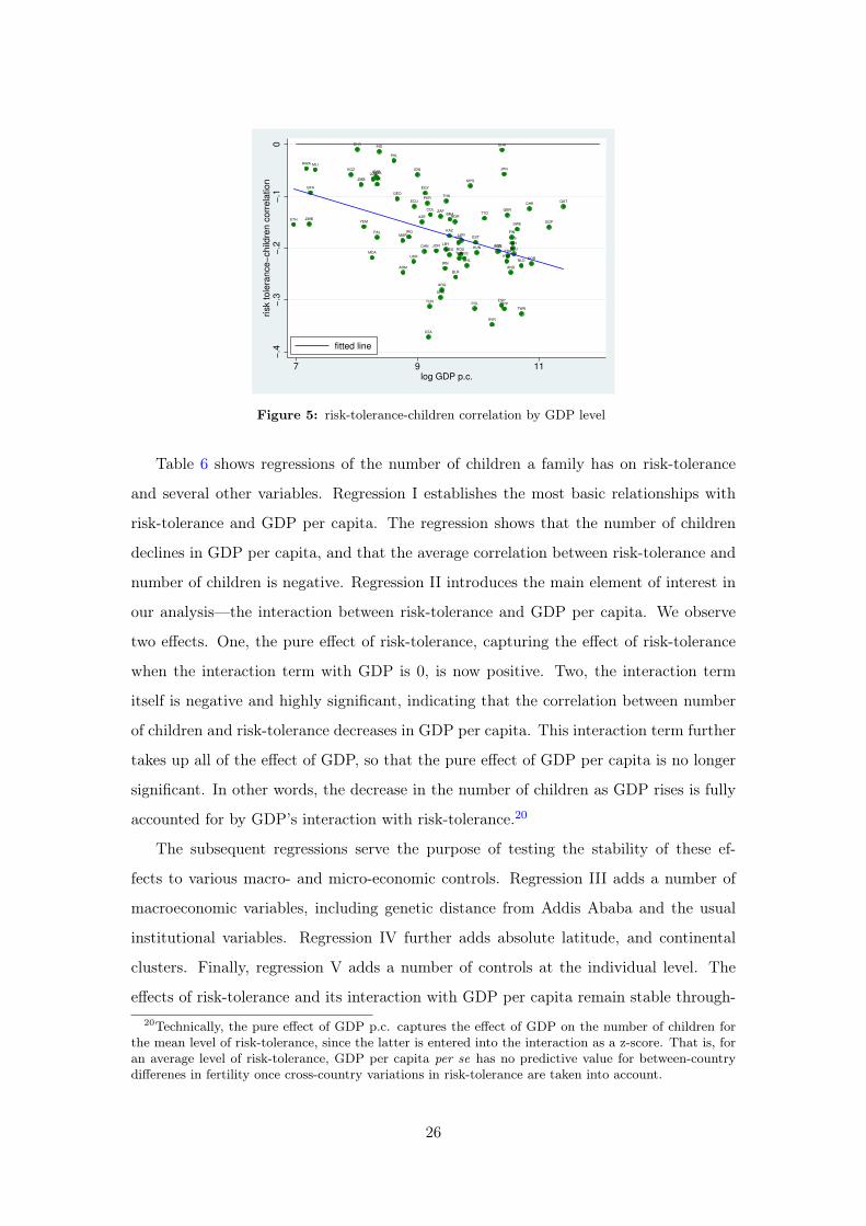
Table 6 shows regressions of the number of children a family has on risk-tolerance
and several other variables. Regression I establishes the most basic relationships with
risk-tolerance and GDP per capita. The regression shows that the number of children
declines in GDP per capita, and that the average correlation between risk-tolerance and
number of children is negative. Regression II introduces the main element of interest in
our analysis—the interaction between risk-tolerance and GDP per capita. We observe
two effects. One, the pure effect of risk-tolerance, capturing the effect of risk-tolerance
when the interaction term with GDP is 0, is now positive. Two, the interaction term
itself is negative and highly significant, indicating that the correlation between number
of children and risk-tolerance decreases in GDP per capita. This interaction term further
takes up all of the effect of GDP, so that the pure effect of GDP per capita is no longer
significant. In other words, the decrease in the number of children as GDP rises is fully
accounted for by GDP’s interaction with risk-tolerance.20
The subsequent regressions serve the purpose of testing the stability of these ef-
fects to various macro- and micro-economic controls. Regression III adds a number of
macroeconomic variables, including genetic distance from Addis Ababa and the usual
institutional variables. Regression IV further adds absolute latitude, and continental
clusters. Finally, regression V adds a number of controls at the individual level. The
effects of risk-tolerance and its interaction with GDP per capita remain stable through-20Technically, the pure effect of GDP p.c. captures the effect of GDP on the number of children for
the mean level of risk-tolerance, since the latter is entered into the interaction as a z-score. That is, foran average level of risk-tolerance, GDP per capita per se has no predictive value for between-countrydifferenes in fertility once cross-country variations in risk-tolerance are taken into account.
26
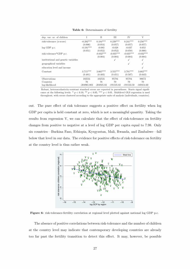
Table 6: Determinants of fertility
dep. var: nr. of children I II III IV V
risk-tolerance (z-score) -0.292*** 0.184*** 0.239*** 0.241*** 0.256***(0.006) (0.054) (0.057) (0.057) (0.057)
log GDP p.c. -0.191*** -0.083 -0.028 -0.037 0.053(0.051) (0.052) (0.052) (0.058) (0.068)
risk-tolerance*GDP p.c. -0.032*** -0.035*** -0.035*** -0.032***(0.004) (0.004) (0.004) (0.004)
institutional and genetic variables X X X
geographical variables X X
education level and income X
Constant 3.715*** 3.665*** 3.555*** 3.781*** 3.682***(0.481) (0.483) (0.451) (0.507) (0.643)
Observations 102531 102531 95784 95784 88672Countries 76 76 70 70 70log-likelihood -204965.003 -204925.02 -191535.02 -191533.50 -169454.60
Robust, heteroscedasticity-resistant standard errors are reported in parentheses. Starts signal signifi-cance at the following levels: * p < 0.10, ** p < 0.05, *** p < 0.01. Multilevel OLS regression is usedthroughout, with errors clustered according to the appropriate units of analysis (individuals, countries).
out. The pure effect of risk tolerance suggests a positive effect on fertility when log
GDP per capita is held constant at zero, which is not a meaningful quantity. Taking the
results from regression V, we can calculate that the effect of risk-tolerance on fertility
changes from positive to negative at a level of log GDP per capita equal to 7.98. Only
six countries—Burkina Faso, Ethiopia, Kyrgyzstan, Mali, Rwanda, and Zimbabwe—fall
below that level in our data. The evidence for positive effects of risk-tolerance on fertility
at the country level is thus rather weak.
DZA
DZA
DZA
DZADZA
AZE
ARG
ARG
AUSAUS
AUS
AUS
AUS
BRA
BRA BRA
BRA
BRA
BRA
BGR
BGR
BGR
BGR
BGR
BGR
BGR
BGR
BGR
BLR
BLR
BLR
BLRBLR
BLR
BLR
CAN
CAN
CAN
CAN
CAN
CANCAN
CAN
CHL
CHN
CHN
CHNCHN
CHN
CHN
CHN
CHN
CHN
CHN
CHN
CHN
CHNCHN
CHN
CHN
COL
COLCOL
COL
COL
COLECU
ECU
ECU
ETHETH
ETH
ETH
EST
EST
FIN
FIN
FIN
FIN
FIN
GEO
GEO
GEO
GEO
GEOGEO
GEO
GEO
PALPAL
DEU
DEU
DEU
DEU
DEU
DEU
DEU
DEU
DEU
DEU
DEU
GHA
GHA
GHA
GHA
GHA
GHA
GHAGHA
GHAHKGHKGHKGHKGHKGHKG
HUN
HUN
HUN
IND
IND
IND
IND
IND
IND
INDIND
IND
IND
IDN
IDN
IDN
IDN
IDN
IRN
IRNIRN
IRN
IRN
IRN
IRN
IRN
IRN
IRN
IRN
IRN
IRN
IRN
IRQ
JPN
JPN
JOR
JOR
JOR
KOR
KOR
KOR
KWT
KWT
KGZ KGZ
KGZKGZ
KGZKGZ
KGZ
LBY
LBY
LBY
LBY
LBY
LBY
LBY
LBY
MYS
MYS
MYS
MYS
MYS
MYSMLI
MLI
MLI
MLI
MLI
MEX
MEX
MEX
MEX
MEX
MEX
MEX
MDA
MAR
MAR
MAR
MAR
MAR
MAR
MAR
MAR
NLD
NLD
NLD
NLD
NLD
NLD
NLD
NZL
NZL NZL
NORNOR
NOR
NOR
NOR
PAK
PAK
PAK
ROU
ROU
ROU
ROU
ROU
RUS
RWA
RWA RWA
RWA
RWA
RWA
RWARWARWA
RWA
RWA
VNM
SVNSVN
SVN
ZAF
ZAF
ZAFZAF
ZAF
ZAF
ZAF
ZAF
ESP
ESP
SWE
SWESWE
SWE
CHE
TUN
TUN
TUN
TUN
TUN
TUN
TUN
TUN
TUN
TUN
TUR
TURUKR
UKR
EGY
EGY
EGYEGY
EGY
EGY
EGY
EGY
EGY
EGY
EGY
EGY
EGY
GBR
BFA
BFA
BFA
UZB
UZB
UZB
UZB
UZB
UZBUZB
UZB
UZB
UZB
UZB
YEM
YEM
YEM
YEM
YEM
SRB
ZMB
ZMB
ZMB
ZMB
ZMB
ZMB
ZMB
ZMBZMB
−.6
−.4
−.2
0.2
risk t
ole
ran
ce
−ch
ildre
n c
orr
ela
tio
n (
reg
ion
al)
−16 −15 −14 −13 −12 −11 −10 −9log GCP by region
fitted line
Figure 6: risk-tolerance-fertility correlation at regional level plotted against national log GDP p.c.
The absence of positive correlations between risk-tolerance and the number of children
at the country level may indicate that contemporary developing countries are already
too far past the fertility transition to detect this effect. It may, however, be possible
27
to still find such positive correlations at the sub-national level, given how rural regions
typically lag behind more urbanized regions in terms of the fertility transition. Figure 6
shows the correlation of risk-tolerance and number of children, plotted against a measure
of income per capita at the regional level.21 We restrict ourselves to regions for which we
have at least 60 observations, in order to avoid outliers in the correlation deriving from
small sample sizes (the results are stable to using smaller or larger cutoff points). The
correlation is negative as expected and highly significant (r = −0.341, p < 0.001, N =
312). We also observe a number of positive correlations especially in poor and middle
income countries. This supports prediction GM3 in its stronger form.
5 Conclusion
We set out to test the predictions of two growth models that describe risk-tolerance as
endogenously determined by growth processes. We found considerable support for the
main mechanism underlying the models, that risk-tolerance acts as a determinant of en-
trepreneurship. More originally, we found evidence of a risk-income paradox. The latter
consists of a positive correlation between risk-tolerance and income within countries, in
combination with a negative correlation between aggregate risk-tolerance and GDP per
capita between countries. The latter may seem surprising in light of a view of developing
countries as being extremely risk averse, which prevailed until very recently (Haushofer
and Fehr, 2014). Nevertheless, this result is highly consistent with previous evidence
based on students (Rieger et al., 2014; Vieider et al., 2015). It is also in agreement
with the predictions derived from the model of Galor and Michalopoulos (2012), and the
general spirit of Doepke and Zilibotti (2014).
A central element in the model of Doepke and Zilibotti (2014) is that risk-tolerance is
instilled by parents into their children to prepare them for the environment they will face
as adults. In this sense, riskiness of the environment may be one of the factors inducing
parents to instill risk-tolerance into their children. At first sight, this interpretation of
their model appears to present parallels to theories from biology adopted into psychol-
ogy. According to so-called life-history theory, high environmental uncertainty about the21We assembled the income per capita data at the regional level from the gross-cell-product (GCP)
data assembled and discussed by Nordhaus (2006). The graph excludes a few extreme outliers on theGCP scale, generally found in petrolium-producing regions. The online appendix provides details onthe assembly of the GCP data, and a stability analysis.
28
future induces people to take large amounts of risk in order to maximize their immediate
payoffs (Hill, Ross and Low, 1997). In particular, Wilson and Daly (1997) showed a num-
ber of correlations between the average life expectancy in Chicago neighborhoods and
risk-taking behaviors such as homicide rates, age at first child, and number of children.
Notice, however, how life history theory postulates that individuals themselves exhibit a
reaction to the riskiness of the environment. This is different from a setup where parents
socialize children, and indeed it results in predictions of differential riskiness by neigh-
bourhoods rather than whole countries. These predictions do not appear to be borne
out by our data, given the positive correlation between risk-tolerance and income, and
thus seem generally in contradiction to the within-country effects we find.
The most important differences between the models of Galor and Michalopoulos
(2012) and Doepke and Zilibotti (2014) concern the transmission of risk-tolerance. In
particular, Galor and Michalopoulos (2012) take no explicit stand on the mechanism
through which risk-tolerance is transmitted. Some form of vertical transmission is, how-
ever, central to their model, given the role played by fertility. Fertility plays no explicit
role in the model of Doepke and Zilibotti (2014), who on the other hand put the em-
phasis on parents’ decision to instill beneficial levels of risk-tolerance into their children.
Testing the underlying mechanisms, we did indeed found strong support for the fertility
channel postulated by Galor and Michalopoulos (2012), while we did not find any strong
support for the mechanisms modeled by Doepke and Zilibotti (2014).
The empirical evidence on how intergenerational transmission works is still limited.
There is clear evidence that the risk-tolerance of parents and children is correlated (Kim-
ball et al., 2009; Dohmen et al., 2012). While Cesarini, Dawes, Johannesson, Lichtenstein
and Wallace (2009) and Zhong, Chew, Set, Zhang, Xue, Sham, Ebstein and Israel (2009)
have shown that some of the intergenerational correlation in risk-tolerance appears to
have genetic origins, the two studies came up with radically different estimates about
the strength of this effect, and a genetic component does not exclude cultural transmis-
sion. Notwithstanding the careful examination of intergenerational correlations carried
out by Dohmen et al. (2012), the evidence for purely cultural mechanisms remains weak.
There are, however, other indications in the empirical literature that risk-tolerance may
be shaped by the economic environment. Malmendier and Nagel (2011) showed that
macroeconomic events during a person’s youth may have lasting effects on their risk-
tolerance. Booth and Nolen (2012) found systematic differences in the risk-tolerance
29

of girls from single sex schools and mixed sex schools, which are suggestive of hori-
zontal social transmission of risk-tolerance. Bacon, Conte and Moffatt (2014) showed
that assimilation plays a role in explaining the correlation in the risk-tolerance of cou-
ples. More work quantifying the relative strength of different transmission mechanisms
is clearly needed in order to calibrate this aspect of the models.
30
References
Andersen, Steffen, Glenn W. Harrison, Morten Igel Lau, and E. Elisabet Rutström (2010)
‘Preference heterogeneity in experiments: Comparing the field and laboratory.’ Journal
of Economic Behavior & Organization 73(2), 209–224
Andersson, Ola, Jean-Robert Tyran, Erik Wengström, and Håkan J. Holm (2016) ‘Risk
Aversion Relates to Cognitive Ability: Preferences or Noise?’ Journal of the European
Economic Association 14(5), 1129–1154
Ashraf, Quamrul, and Oded Galor (2013) ‘The “Out of Africa” Hypothesis, Human
Genetic Diversity, and Comparative Economic Development.’ The American Economic
Review 103(1), 1–46
Ashraf, Quamrul H, and Oded Galor (2018) ‘The macrogenoeconomics of comparative
development.’ Journal of Economic Literature 56(3), 1119–55
Bacon, Philomena M., Anna Conte, and Peter G. Moffatt (2014) ‘Assortative mating on
risk attitude.’ Theory and Decision 77(3), 389–401
Barro, Robert J. (1991) ‘Economic Growth in a Cross-Section of Countries.’ Quarterly
Journal of Economics
Becker, Anke, Thomas Dohmen, Benjamin Enke, and Armin Falk (2015) ‘The Ancient
Origins of the Cross-Country Heterogeneity in Risk Preferences.’ Working Paper
Becker, Gary S. (1960) ‘An Economic Analysis of Fertility.’ In ‘Demographic and Eco-
nomic Change in Developed Countries’ (209: Princeton University Press) pp. 209–240
Becker, Gary S., Kevin M. Murphy, and Robert Tamura (1990) ‘Human Capital, Fertility,
and Economic Growth.’ Journal of Political Economy 98(5), S12–S37
Benjamin, Daniel J., Sebastian A. Brown, and Jesse M. Shapiro (2013) ‘Who Is ‘Be-
havioral’? Cognitive Ability and Anomalous Preferences.’ Journal of the European
Economic Association 11(6), 1231–1255
Binswanger, Hans P. (1980) ‘Attitudes toward Risk: Experimental Measurement in Rural
India.’ American Journal of Agricultural Economics 62(3), 395–407
Bisin, Alberto, and Thierry Verdier (2001) ‘The Economics of Cultural Transmission and
the Dynamics of Preferences.’ Journal of Economic Theory 97(2), 298–319
Bonin, Holger, Thomas Dohmen, Armin Falk, David Huffmann, and Uwe Sunde (2007)
‘Cross-sectional earnings risk and occupational sorting: The role of risk attitudes.’
Labour Economics 14(6), 926–937
31
Booij, Adam S., Bernard M. S. van Praag, and Gijs van de Kuilen (2010) ‘A paramet-
ric analysis of prospect theory’s functionals for the general population.’ Theory and
Decision 68(1-2), 115–148
Booth, Alison L., and Patrick Nolen (2012) ‘Gender differences in risk behaviour: does
nurture matter?’ The Economic Journal 122(558), F56–F78
Bowles, Samuel (1998) ‘Endogenous preferences: The cultural consequences of markets
and other economic institutions.’ Journal of Economic Literature 36(1), 75–111
Cardenas, Juan Camilo, and Jeffrey Carpenter (2013) ‘Risk attitudes and economic well-
being in Latin America.’ Journal of Development Economics 103, 52–61
Cesarini, David, Christopher T. Dawes, Magnus Johannesson, Paul Lichtenstein, and
Björn Wallace (2009) ‘Genetic Variation in Preferences for Giving and Risk Taking.’
Quarterly Journal of Economics 124(2), 809–842
Charles, Kerwin Kofi, and Erik Hurst (2003) ‘The Correlation of Wealth Across Gener-
ations.’ Journal of Political Economy 111(6), 1155–1182
Clark, Gregory (2007) A Farewell to Alms: A Brief Economic History of the World
(Princeton and Oxford: Princeton University Press)
Clark, Gregory, and Gillian Hamilton (2006) ‘Survival of the Richest: The Malthusian
Mechanism in Pre-Industrial England.’ Journal of Economic History 66(3), 707–736
Cohen, Barney (1998) ‘The emerging fertility transition in sub-Saharan Africa.’ World
Development 26(8), 1431–1461
Cramer, J. S., Joop Hartog, N. Jonker, and C. M. van Praag (2002) ‘Low Risk Aversion
Encourages the Choices for Entrepreneurship: An Empirical Test of a Truism.’ Journal
of Economic Behavior & Organization 48, 29–36
Croson, Rachel, and Uri Gneezy (2009) ‘Gender Differences in Preferences.’ Journal of
Economic Literature 47(2), 1–27
di Falco, Salvatore, and Ferdinand M. Vieider (2018) ‘Assimilation in the risk preferences
of spouses.’ Economic Inquiry 56(3), 1809–1816
Doepke, Matthias, and Fabrizio Zilibotti (2008) ‘Occupational choice and the spirit of
capitalism.’ Quarterly Journal of Economics 123(2), 747–793
Doepke, Matthias, and Fabrizio Zilibotti (2014) ‘Culture, Entrepreneurship, and
Growth.’ In ‘Handbook of Economic Growth,’ vol. 2
Doepke, Matthias, and Fabrizio Zilibotti (2017) ‘Parenting with style: Altruism and
32
paternalism in intergenerational preference transmission.’ Econometrica 85(5), 1331–
1371
Dohmen, Thomas, Armin Falk, David Huffman, and Uwe Sunde (2010) ‘Are Risk
Aversion and Impatience Related to Cognitive Ability?’ American Economic Review
100, 1238–1260
(2012) ‘The Intergenerational Transmission of Risk and Trust Attitudes.’ Review of
Economic Studies 70(2), 645–677
Dohmen, Thomas, Armin Falk, David Huffman, Uwe Sunde, Jürgen Schupp, and Gert G.
Wagner (2011) ‘Individual Risk Attitudes: Measurement, Determinants, and Behav-
ioral Consequences.’ Journal of the European Economic Association 9(3), 522–550
Falk, Armin, Anke Becker, Thomas Dohmen, Benjamin Enke, David Huffman, and Uwe
Sunde (2018) ‘Global evidence on economic preferences.’ The Quarterly Journal of
Economics, forthcoming
Fehr-Duda, Helga, and Thomas Epper (2012) ‘Probability and Risk: Foundations and
Economic Implications of Probability-Dependent Risk Preferences.’ Annual Review of
Economics 4(1), 567–593
Galizzi, Matteo M., Sara R. Machado, and Raffaele Miniaci (2016) ‘Temporal Stability,
Cross-Validity, and External Validity of Risk Preferences Measures: Experimental
Evidence from a UK Representative Sample.’ SSRN Scholarly Paper ID 2822613, Social
Science Research Network, Rochester, NY, August
Gallup, John Luke, Jeffrey D. Sachs, and Andrew D. Mellinger (1999) ‘Geography and
Economic Development.’ International Regional Science Review 22(2), 179–232
Galor, Oded, and David N. Weil (2000) ‘Population, Technology, and Growth: From
Malthusian Stagnation to the Demographic Transition and beyond.’ American Eco-
nomic Review 90(4), 806–828
Galor, Oded, and Marc Klemp (2019) ‘Human genealogy reveals a selective advantage
to moderate fecundity.’ Nature Ecology & Evolution 3, 853–857
Galor, Oded, and Omer Moav (2002) ‘Natural Selection and the Origin of Economic
Growth.’ Quarterly Journal of Economics 117(4), 1133–1191
Galor, Oded, and Ömer Özak (2016) ‘The agricultural origins of time preference.’ Amer-
ican Economic Review 106(10), 3064–3103
Galor, Oded, and Stelios Michalopoulos (2012) ‘Evolution and the Growth Process:
33
Natural Selection of Entrepreneurial Traits.’ Journal of Economic Theory 147(2), 759–
780
Galor, Oded, and Viacheslav Savitskiy (2018) ‘Climatic Roots of Loss Aversion.’ Tech-
nical Report
Garenne, Michel, and Veronique Joseph (2002) ‘The Timing of the Fertility Transition
in Sub-Saharan Africa.’ World Development 30(10), 1835–1843
Gloede, Oliver, Lukas Menkhoff, and Hermann Waibel (2015) ‘Shocks, Individual Risk
Attitude, and Vulnerability to Poverty among Rural Households in Thailand and Viet-
nam.’ World Development 71, 54–78
Goodman, Anna, Ilona Koupil, and David W. Lawson (2012) ‘Low fertility increases
descendant socioeconomic position but reduces long-term fitness in a modern post-
industrial society.’ Proceedings of the Royal Society B
Görlitz, Katja, and Marcus Tamm (2015) ‘Parenthood and Risk Preferences.’ SSRN
Scholarly Paper ID 2618442, Social Science Research Network, Rochester, NY, April
Hardeweg, Bernd, Lukas Menkhoff, and Hermann Waibel (2013) ‘Experimentally Val-
idated Survey Evidence on Individual Risk Attitudes in Rural Thailand.’ Economic
Development and Cultural Change 61(4), 859–888
Haushofer, Johannes, and Ernst Fehr (2014) ‘On the psychology of poverty.’ Science
344(6186), 862–867
Hill, Elizabeth M, Lisa Thomson Ross, and Bobbi S Low (1997) ‘The role of future
unpredictability in human risk-taking.’ Human Nature 8(4), 287
Hopland, Arnt O, Egil Matsen, and Bjarne Strøm (2016) ‘Income and choice under risk.’
Journal of Behavioral and Experimental Finance 12, 55–64
Keefer, Philip, and Stephen Knack (1997) ‘Why Don’t Poor Countries Catch up? a
Cross-National Test of an Institutional Explanation.’ Economic Inquiry 35(3), 590–
602
Kimball, Miles S., Claudia R. Sahm, and Matthew D. Shapiro (2009) ‘Risk Preferences
in the PSID: Individual Imputations and Family Covariation.’ American Economic
Review, Papers and Proceedings 99(2), 363–368
Klasing, Mariko J. (2014) ‘Cultural change, risk-taking behavior and implications for
economic development.’ Journal of Development Economics 110, 158–169
La Porta, Rafael, Florencio López-de Silanes, Andrei Shleifer, and Robert Vishny (1998)
34
‘Law and Finance.’ Journal of Political Economy 106(6), 1113–1155
Levine, Ross (1998) ‘The Legal Environment, Banks, and Long-Run Economic Growth.’
Journal of Money, Credit and Banking 30(3), 596–613
L’Haridon, Olivier, and Ferdinand M. Vieider (2019) ‘All over the map: A worldwide
comparison of risk preferences.’ Quantitative Economics 10, 185?–215
Lönnqvist, Jan-Erik, Markku Verkasalo, Gari Walkowitz, and Philipp C. Wichardt (2015)
‘Measuring individual risk attitudes in the lab: Task or ask? An empirical comparison.’
Journal of Economic Behavior & Organization 119, 254–266
Malmendier, Ulrike, and Stefan Nagel (2011) ‘Depression Babies: Do Macroeconomic
Experiences Affect Risk Taking?*.’ The Quarterly Journal of Economics 126(1), 373–
416
Moulton, Brent R. (1986) ‘Random group effects and the precision of regression esti-
mates.’ Journal of Econometrics 32(3), 385–397
Nordhaus, William D. (2006) ‘Geography and macroeconomics: New data and new find-
ings.’ Proceedings of the National Academy of Sciences of the United States of America
103(10), 3510–3517
Noussair, Charles N., Stefan Trautmann, and Gijs van de Kuilen (2014) ‘Higher Order
Risk Attitudes, Demographics, and Financial Decisions.’ Review of Economic Studies
21(1), 325–355
Rieger, Marc Oliver, Mei Wang, and Thorsten Hens (2014) ‘Risk Preferences Around
the World.’ Management Science 61(3), 637 – 648
Robinson, W. (1950) ‘Ecological correlations and the behavior of individuals.’ American
Sociological Review 15, 351–357
Sala-i Martin, Xavier X. (1996) ‘The Classical Approach to Convergence Analysis.’ Eco-
nomic Journal 106(437), 1019–36
Schmidt, Lucie (2008) ‘Risk preferences and the timing of marriage and childbearing.’
Demography 45(2), 439–460
Shaw, Kathryn L. (1996) ‘An empirical analysis of risk aversion and income growth.’
Journal of Labor Economics 14(4), 626–653
Snijders, Tom A. B., and Roel J. Bosker (2012) Multilevel Analysis: An Introduction to
Basic and Advanced Multilevel Modeling, 2nd ed. (London: Sage PUblications)
Tanaka, Tomomi, Colin F. Camerer, and Quang Nguyen (2010) ‘Risk and Time Prefer-
35
ences: Linking Experimental and Household Survey Data from Vietnam.’ American
Economic Review 100(1), 557–571
Vieider, Ferdinand M., Abebe Beyene, Randall A. Bluffstone, Sahan Dissanayake, Zenebe
Gebreegziabher, Peter Martinsson, and Alemu Mekonnen (2018) ‘Measuring risk pref-
erences in rural Ethiopia.’ Economic Development and Cultural Change 66(3), 417–446
Vieider, Ferdinand M., Mathieu Lefebvre, Ranoua Bouchouicha, Thorsten Chmura, Rus-
tamdjan Hakimov, Michal Krawczyk, and Peter Martinsson (2015) ‘Common compo-
nents of risk and uncertainty attitudes across contexts and domains: Evidence from
30 countries.’ Journal of the European Economic Association 13(3), 421–452
Vieider, Ferdinand M., Peter Martinsson, Nam Pham Khanh, and Nghi Truong (2019)
‘Risk Preferences and Development Revisited.’ Theory & Decision 86, 1–21
von Gaudecker, Hans-Martin, Arthur van Soest, and Erik Wengström (2011) ‘Hetero-
geneity in Risky Choice Behaviour in a Broad Population.’ American Economic Review
101(2), 664–694
Wilson, M., and M. Daly (1997) ‘Life expectancy, economic inequality, homicide, and
reproductive timing in Chicago neighbourhoods.’ BMJ : British Medical Journal
314(7089), 1271–1274
Zeger, Scott L., Kung-Yee Liang, and Paul S. Albert (1988) ‘Models for Longitudinal
Data: A Generalized Estimating Equation Approach.’ Biometrics 44(4), 1049–1060
Zhong, Songfa, Soo Hong Chew, Eric Set, Junsen Zhang, Hong Xue, Pak C. Sham,
Richard P. Ebstein, and Salomon Israel (2009) ‘The Heritability of Attitude Toward
Economic Risk.’ Twin Research and Human Genetics 12(1), 103–107
36