Embed Size (px)
Citation preview
Principles and Practiceof
Earth Electrode Measurements
Document Information:Author: Whitham D. ReeveRevision: 0.0 (initial draft 06/18/2002)
0.1 (working draft 10/05/2003)0.2 (additional work 10/07/2003)0.3 (editorial revisions 05/09/2004)0.4 (added Slope Field Data Form, 10/01/2004)1.0 (added appendices and issued, 10/13/2004)1.1 (editorial revisions and added soil resistivity section, 08/01/2008)
Principles and Practice of Earth Electrode Measurements
Reeve Engineers 2008, File: Ground Testing R1-1.doc, Page 1
1. Introduction
This application note describes principles and methods for measuring the resistance to remoteearth of grounding systems (earth electrode systems) used in telecommunications facilities. Thisnote does not describe all earth electrode measurement techniques but only those found throughfield experience to be most useful and consistent. While test equipment is in the field forresistance measurements, it is convenient to also measure soil resistivity; therefore, thisapplication note also describes soil resistivity measurements.
This information largely is based on the author’s experience and may or may not be correct, safeor useful. None of the information provided in this document is professional engineering advice.The most important things to remember are: Use common sense and make your measurements ina safe manner. Do not rely on this document for safety information. Always be alert andconscious of your surroundings.
You use the information in this document at your own risk. Information in this document isprovided as-is. It is only for the reader’s consideration and study and includes no claimwhatsoever as to usefulness, accuracy of content, or accuracy of information.
2. Ground Measurement Principles
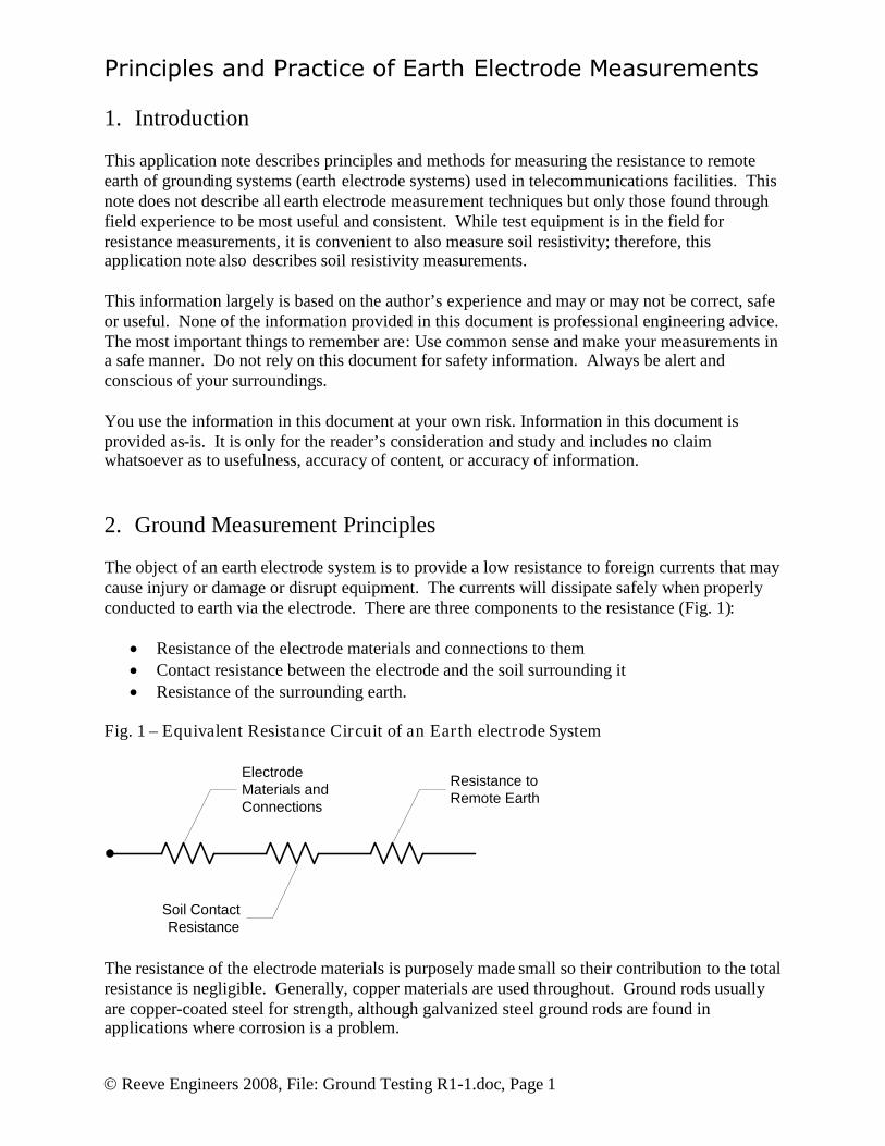
The object of an earth electrode system is to provide a low resistance to foreign currents that maycause injury or damage or disrupt equipment. The currents will dissipate safely when properlyconducted to earth via the electrode. There are three components to the resistance (Fig. 1):
Resistance of the electrode materials and connections to them Contact resistance between the electrode and the soil surrounding it Resistance of the surrounding earth.
Fig. 1 – Equivalent Resistance Circuit of an Earth electrode System
ElectrodeMaterials andConnections
Soil ContactResistance
Resistance toRemote Earth
The resistance of the electrode materials is purposely made small so their contribution to the totalresistance is negligible. Generally, copper materials are used throughout. Ground rods usuallyare copper-coated steel for strength, although galvanized steel ground rods are found inapplications where corrosion is a problem.

Principles and Practice of Earth Electrode Measurements
Reeve Engineers 2008, File: Ground Testing R1-1.doc, Page 2
The contact resistance between the electrode and soil is negligible if the electrode materials areclean and unpainted when installed and the earth is packed firmly. Even rusted steel ground rodshave little contact resistance because the iron oxide readily soaks up water and has less resistancethan most soils (however, rusted ground rods may eventually rust apart in which case theireffectiveness is greatly reduced).
Generally, the resistance of the surrounding earth will be the largest of the three components. Anearth electrode system buried in the earth radiates current in all directions and eventuallydissipates some distance away depending on the soil’s resistance to current flow, as indicated byits resistivity.
An earth electrode system consists of all interconnected buried metallic components includingground rods, ground grids, buried metal plates, radial ground systems and buried horizontalwires, water well casings and buried metallic water lines, concrete encased electrodes (Ufergrounds), and building structural steel.
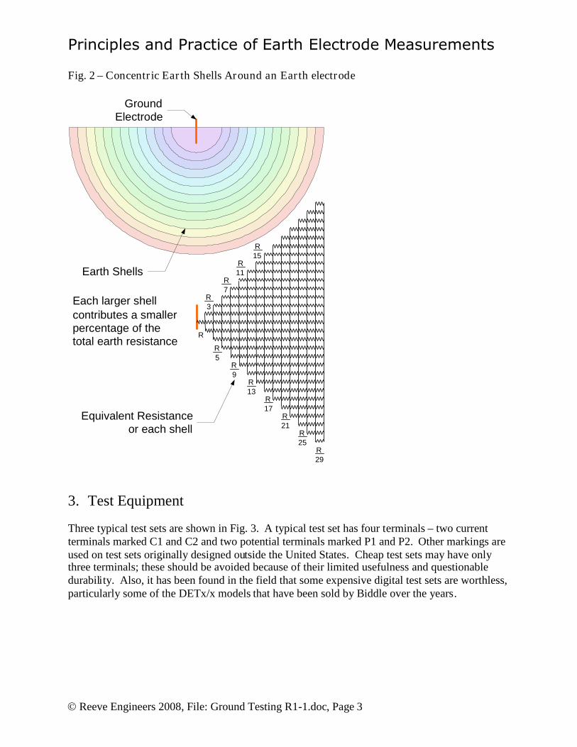
The earth electrode can be thought of as being surrounding by shells of earth, each of the samethickness (Fig. 2). The shell closest to the electrode has the smallest surface area and offers thegreatest resistance. The next shell has larger area and lower resistance, and so on. A distanceeventually will be reached where the additional earth shells do not add significantly to theresistance. Earth electrode resistance is measured to remote earth, which is the earth outside theelectrode’s influence. A larger electrode system requires greater distance before its influencedecreases to a negligible level.
Another way of thinking about the earth shells is as parallel resistances. The closest shell hassome unit resistance. The next larger shell has more surface area so it is equivalent to severalunit resistances in parallel. Each larger shell has smaller equivalent resistance due to moreparallel resistances.
The resistance of the surrounding earth depends on the soil resistivity. Soil resistivity ismeasured in ohm-meters (ohm-m) or ohm-centimeters (ohm-cm) and is the resistance betweentwo opposite faces of a 1 meter or 1 centimeter cube of the soil material. The soil resistivitydepends on the type of soil, salt concentration and its moisture content and temperature. Frozenand very dry soils are a good insulators (have high resistivity) and are ineffective with earthelectrodes. The resistivity of many soil types is provided in Section 8.
Principles and Practice of Earth Electrode Measurements
Reeve Engineers 2008, File: Ground Testing R1-1.doc, Page 3
Fig. 2 – Concentric Earth Shells Around an Earth electrode
R
R3
R5
R7
R9
R13
R17
R21
R25
R29
R11
R15
Each larger shellcontributes a smallerpercentage of thetotal earth resistance
Earth Shells
GroundElectrode
Equivalent Resistanceor each shell
3. Test Equipment
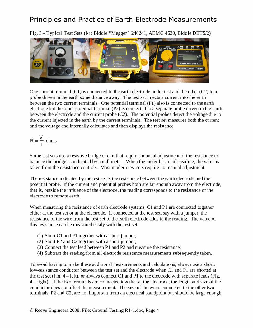
Three typical test sets are shown in Fig. 3. A typical test set has four terminals – two currentterminals marked C1 and C2 and two potential terminals marked P1 and P2. Other markings areused on test sets originally designed outside the United States. Cheap test sets may have onlythree terminals; these should be avoided because of their limited usefulness and questionabledurability. Also, it has been found in the field that some expensive digital test sets are worthless,particularly some of the DETx/x models that have been sold by Biddle over the years.
Principles and Practice of Earth Electrode Measurements
Reeve Engineers 2008, File: Ground Testing R1-1.doc, Page 4
Fig. 3 – Typical Test Sets (l-r: Biddle “Megger” 240241, AEMC 4630, Biddle DET5/2)
One current terminal (C1) is connected to the earth electrode under test and the other (C2) to aprobe driven in the earth some distance away. The test set injects a current into the earthbetween the two current terminals. One potential terminal (P1) also is connected to the earthelectrode but the other potential terminal (P2) is connected to a separate probe driven in the earthbetween the electrode and the current probe (C2). The potential probes detect the voltage due tothe current injected in the earth by the current terminals. The test set measures both the currentand the voltage and internally calculates and then displays the resistance
IV
R ohms
Some test sets use a resistive bridge circuit that requires manual adjustment of the resistance tobalance the bridge as indicated by a null meter. When the meter has a null reading, the value istaken from the resistance controls. Most modern test sets require no manual adjustment.
The resistance indicated by the test set is the resistance between the earth electrode and thepotential probe. If the current and potential probes both are far enough away from the electrode,that is, outside the influence of the electrode, the reading corresponds to the resistance of theelectrode to remote earth.
When measuring the resistance of earth electrode systems, C1 and P1 are connected togethereither at the test set or at the electrode. If connected at the test set, say with a jumper, theresistance of the wire from the test set to the earth electrode adds to the reading. The value ofthis resistance can be measured easily with the test set:
(1) Short C1 and P1 together with a short jumper;(2) Short P2 and C2 together with a short jumper;(3) Connect the test lead between P1 and P2 and measure the resistance;(4) Subtract the reading from all electrode resistance measurements subsequently taken.
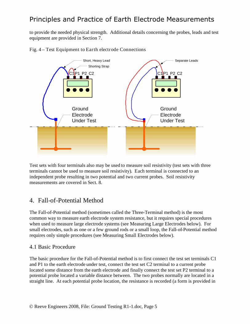
To avoid having to make these additional measurements and calculations, always use a short,low-resistance conductor between the test set and the electrode when C1 and P1 are shorted atthe test set (Fig. 4 – left), or always connect C1 and P1 to the electrode with separate leads (Fig.4 – right). If the two terminals are connected together at the electrode, the length and size of theconductor does not affect the measurement. The size of the wires connected to the other twoterminals, P2 and C2, are not important from an electrical standpoint but should be large enough
Principles and Practice of Earth Electrode Measurements
Reeve Engineers 2008, File: Ground Testing R1-1.doc, Page 5
to provide the needed physical strength. Additional details concerning the probes, leads and testequipment are provided in Section 7.
Fig. 4 – Test Equipment to Earth electrode Connections
C1 C2P2P1
GroundElectrodeUnder Test
Short, Heavy Lead
Shorting Strap
C1 C2P2P1
GroundElectrodeUnder Test
Separate Leads
Test sets with four terminals also may be used to measure soil resistivity (test sets with threeterminals cannot be used to measure soil resistivity). Each terminal is connected to anindependent probe resulting in two potential and two current probes. Soil resistivitymeasurements are covered in Sect. 8.
4. Fall-of-Potential Method
The Fall-of-Potential method (sometimes called the Three-Terminal method) is the mostcommon way to measure earth electrode system resistance, but it requires special procedureswhen used to measure large electrode systems (see Measuring Large Electrodes below). Forsmall electrodes, such as one or a few ground rods or a small loop, the Fall-of-Potential methodrequires only simple procedures (see Measuring Small Electrodes below).
4.1 Basic Procedure
The basic procedure for the Fall-of-Potential method is to first connect the test set terminals C1and P1 to the earth electrode under test, connect the test set C2 terminal to a current probelocated some distance from the earth electrode and finally connect the test set P2 terminal to apotential probe located a variable distance between. The two probes normally are located in astraight line. At each potential probe location, the resistance is recorded (a form is provided in
Principles and Practice of Earth Electrode Measurements
Reeve Engineers 2008, File: Ground Testing R1-1.doc, Page 6
Appendix I for this purpose). The results of these measurements are then plotted to graphicallydetermine the electrode resistance.
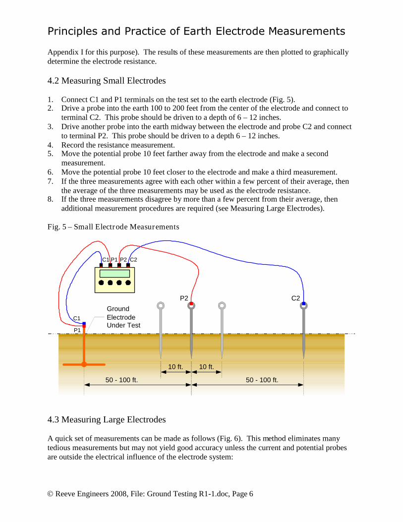
4.2 Measuring Small Electrodes
1. Connect C1 and P1 terminals on the test set to the earth electrode (Fig. 5).2. Drive a probe into the earth 100 to 200 feet from the center of the electrode and connect to
terminal C2. This probe should be driven to a depth of 6 – 12 inches.3. Drive another probe into the earth midway between the electrode and probe C2 and connect
to terminal P2. This probe should be driven to a depth 6 – 12 inches.4. Record the resistance measurement.5. Move the potential probe 10 feet farther away from the electrode and make a second
measurement.6. Move the potential probe 10 feet closer to the electrode and make a third measurement.7. If the three measurements agree with each other within a few percent of their average, then
the average of the three measurements may be used as the electrode resistance.8. If the three measurements disagree by more than a few percent from their average, then
additional measurement procedures are required (see Measuring Large Electrodes).
Fig. 5 – Small Electrode Measurements
C1 C2
P2 C2
P2P1
C1
P1
50 - 100 ft. 50 - 100 ft.
10 ft.10 ft.
GroundElectrodeUnder Test
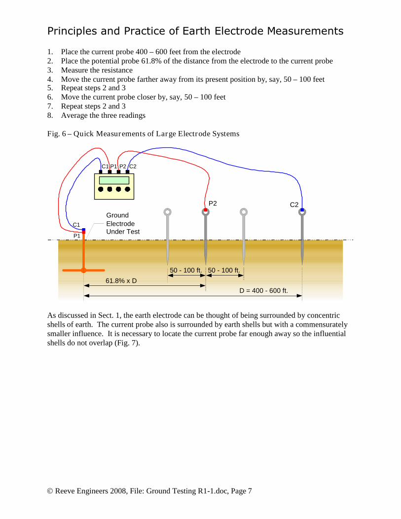
4.3 Measuring Large Electrodes
A quick set of measurements can be made as follows (Fig. 6). This method eliminates manytedious measurements but may not yield good accuracy unless the current and potential probesare outside the electrical influence of the electrode system:
Principles and Practice of Earth Electrode Measurements
Reeve Engineers 2008, File: Ground Testing R1-1.doc, Page 7
1. Place the current probe 400 – 600 feet from the electrode2. Place the potential probe 61.8% of the distance from the electrode to the current probe3. Measure the resistance4. Move the current probe farther away from its present position by, say, 50 – 100 feet5. Repeat steps 2 and 36. Move the current probe closer by, say, 50 – 100 feet7. Repeat steps 2 and 38. Average the three readings
Fig. 6 – Quick Measurements of Large Electrode Systems
C1 C2
P2 C2
P2P1
C1
P1
D = 400 - 600 ft.
50 - 100 ft.
GroundElectrodeUnder Test
50 - 100 ft.
61.8% x D
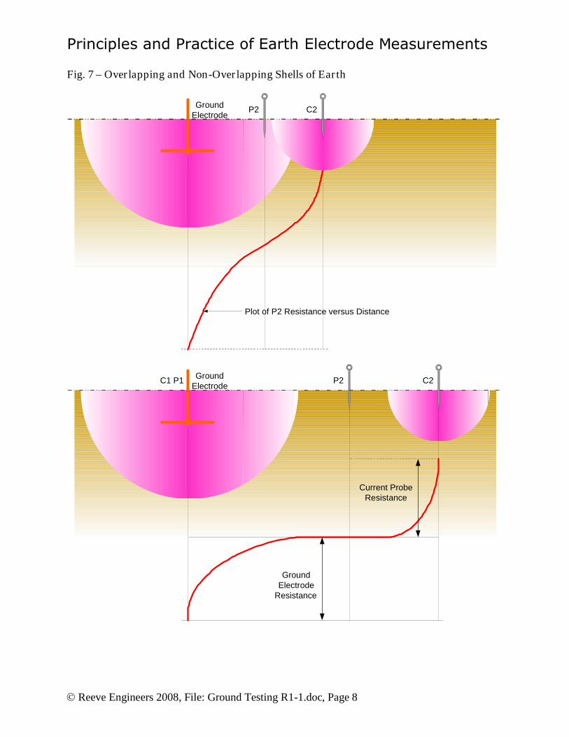
As discussed in Sect. 1, the earth electrode can be thought of being surrounded by concentricshells of earth. The current probe also is surrounded by earth shells but with a commensuratelysmaller influence. It is necessary to locate the current probe far enough away so the influentialshells do not overlap (Fig. 7).
Principles and Practice of Earth Electrode Measurements
Reeve Engineers 2008, File: Ground Testing R1-1.doc, Page 8
Fig. 7 – Overlapping and Non-Overlapping Shells of Earth
GroundElectrode
P2 C2
Plot of P2 Resistance versus Distance
GroundElectrode
P2 C2
Current ProbeResistance
GroundElectrode
Resistance
C1 P1

Principles and Practice of Earth Electrode Measurements
Reeve Engineers 2008, File: Ground Testing R1-1.doc, Page 9
Fall-of-Potential measurements are based on the distance of the current and potential probesfrom the center of the electrode under test. However, the location of the center of the electrodeseldom is known, especially if it consists of numerous types of bonded electrodes such as groundrods, grids, concrete-encased electrodes (Ufer grounds), water well casings and buried radialwires. In these cases, special procedures, such as the Intersecting Curves or Slope methods, arerequired. These are described in later sections.
The farther a probe is placed from the electrode, the smaller the influence. The best distance forthe current probe is at least 10 to 20 times the largest dimension of the electrode (Table 1).However, terrain or obstructions, such as buildings and paved roads, can greatly limit the spaceavailable for measuring larger systems. Nevertheless, acceptable accuracy can be obtained byusing smaller distances in most situations.
Table 1 – Current Probe Distance from Electrode
Maximum ElectrodeDimension (Feet)
Distance to Current Probefrom Electrode Center (Feet)
15 30030 45060 600
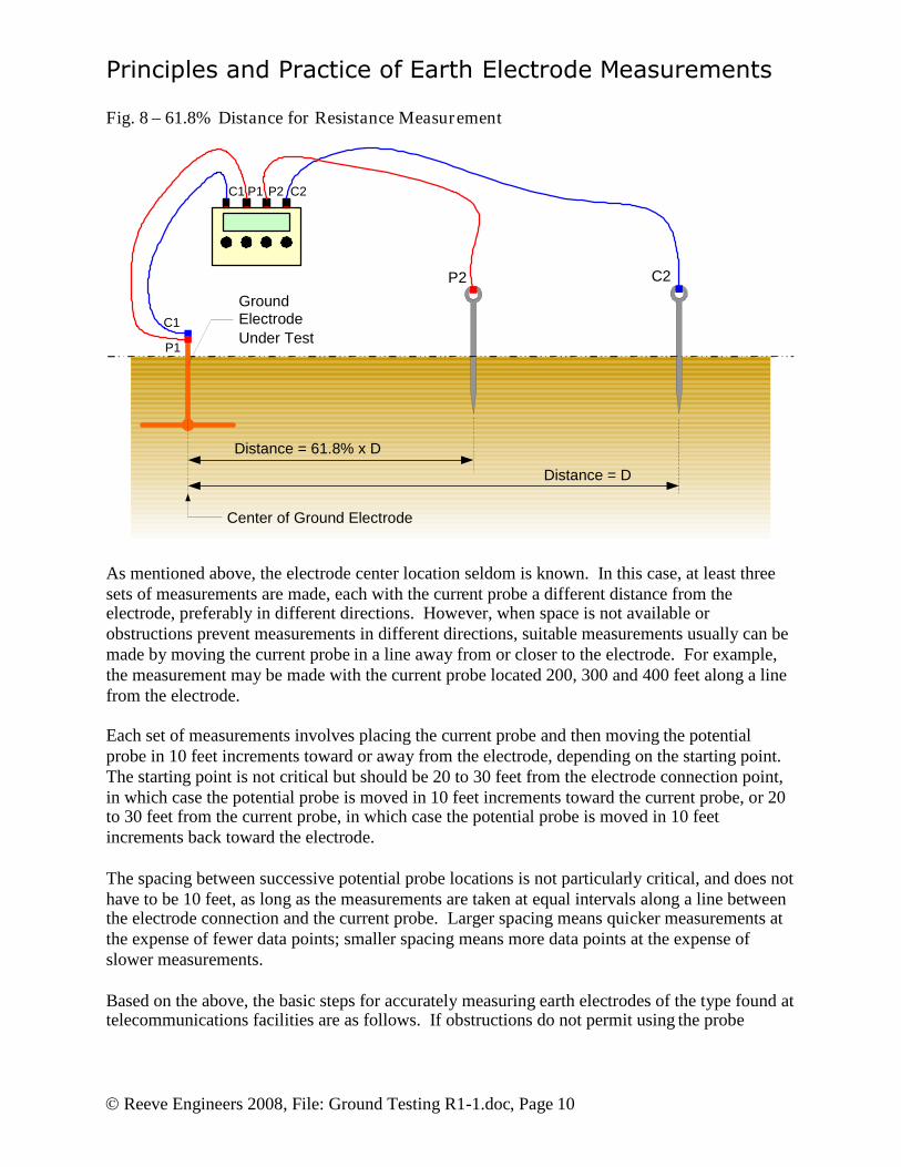
It can be shown (Appendix II) that the actual electrode resistance is measured when the potentialprobe is located 61.8% of the distance between the center of the electrode and the current probe(Fig 8). For example, if the current probe is located 400 feet from the electrode center, then theresistance can be measured with the potential probe located 61.8% x 400 = 247 feet from theelectrode center. The 61.8% measurement point assumes the current and potential probes arelocated in a straight line and the soil is homogeneous (same type of soil surrounding theelectrode area and to a depth equal to 10 times the largest electrode dimension). While the lattercondition is almost never known with certainty, the 61.8% measurement point still providessuitable accuracy for most measurements if other cautionary measures are taken as describedbelow.
Principles and Practice of Earth Electrode Measurements
Reeve Engineers 2008, File: Ground Testing R1-1.doc, Page 10
Fig. 8 – 61.8% Distance for Resistance Measurement
C1 C2
P2 C2
P2P1
C1
P1
Distance = 61.8% x D
Distance = D
GroundElectrodeUnder Test
Center of Ground Electrode
As mentioned above, the electrode center location seldom is known. In this case, at least threesets of measurements are made, each with the current probe a different distance from theelectrode, preferably in different directions. However, when space is not available orobstructions prevent measurements in different directions, suitable measurements usually can bemade by moving the current probe in a line away from or closer to the electrode. For example,the measurement may be made with the current probe located 200, 300 and 400 feet along a linefrom the electrode.
Each set of measurements involves placing the current probe and then moving the potentialprobe in 10 feet increments toward or away from the electrode, depending on the starting point.The starting point is not critical but should be 20 to 30 feet from the electrode connection point,in which case the potential probe is moved in 10 feet increments toward the current probe, or 20to 30 feet from the current probe, in which case the potential probe is moved in 10 feetincrements back toward the electrode.
The spacing between successive potential probe locations is not particularly critical, and does nothave to be 10 feet, as long as the measurements are taken at equal intervals along a line betweenthe electrode connection and the current probe. Larger spacing means quicker measurements atthe expense of fewer data points; smaller spacing means more data points at the expense ofslower measurements.
Based on the above, the basic steps for accurately measuring earth electrodes of the type found attelecommunications facilities are as follows. If obstructions do not permit using the probe
Principles and Practice of Earth Electrode Measurements
Reeve Engineers 2008, File: Ground Testing R1-1.doc, Page 11
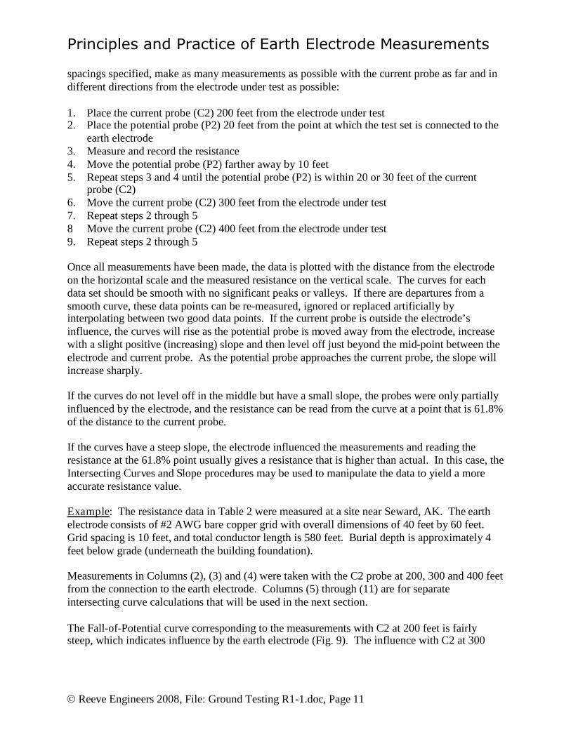
spacings specified, make as many measurements as possible with the current probe as far and indifferent directions from the electrode under test as possible:
1. Place the current probe (C2) 200 feet from the electrode under test2. Place the potential probe (P2) 20 feet from the point at which the test set is connected to the
earth electrode3. Measure and record the resistance4. Move the potential probe (P2) farther away by 10 feet5. Repeat steps 3 and 4 until the potential probe (P2) is within 20 or 30 feet of the current
probe (C2)6. Move the current probe (C2) 300 feet from the electrode under test7. Repeat steps 2 through 58 Move the current probe (C2) 400 feet from the electrode under test9. Repeat steps 2 through 5
Once all measurements have been made, the data is plotted with the distance from the electrodeon the horizontal scale and the measured resistance on the vertical scale. The curves for eachdata set should be smooth with no significant peaks or valleys. If there are departures from asmooth curve, these data points can be re-measured, ignored or replaced artificially byinterpolating between two good data points. If the current probe is outside the electrode’sinfluence, the curves will rise as the potential probe is moved away from the electrode, increasewith a slight positive (increasing) slope and then level off just beyond the mid-point between theelectrode and current probe. As the potential probe approaches the current probe, the slope willincrease sharply.
If the curves do not level off in the middle but have a small slope, the probes were only partiallyinfluenced by the electrode, and the resistance can be read from the curve at a point that is 61.8%of the distance to the current probe.
If the curves have a steep slope, the electrode influenced the measurements and reading theresistance at the 61.8% point usually gives a resistance that is higher than actual. In this case, theIntersecting Curves and Slope procedures may be used to manipulate the data to yield a moreaccurate resistance value.
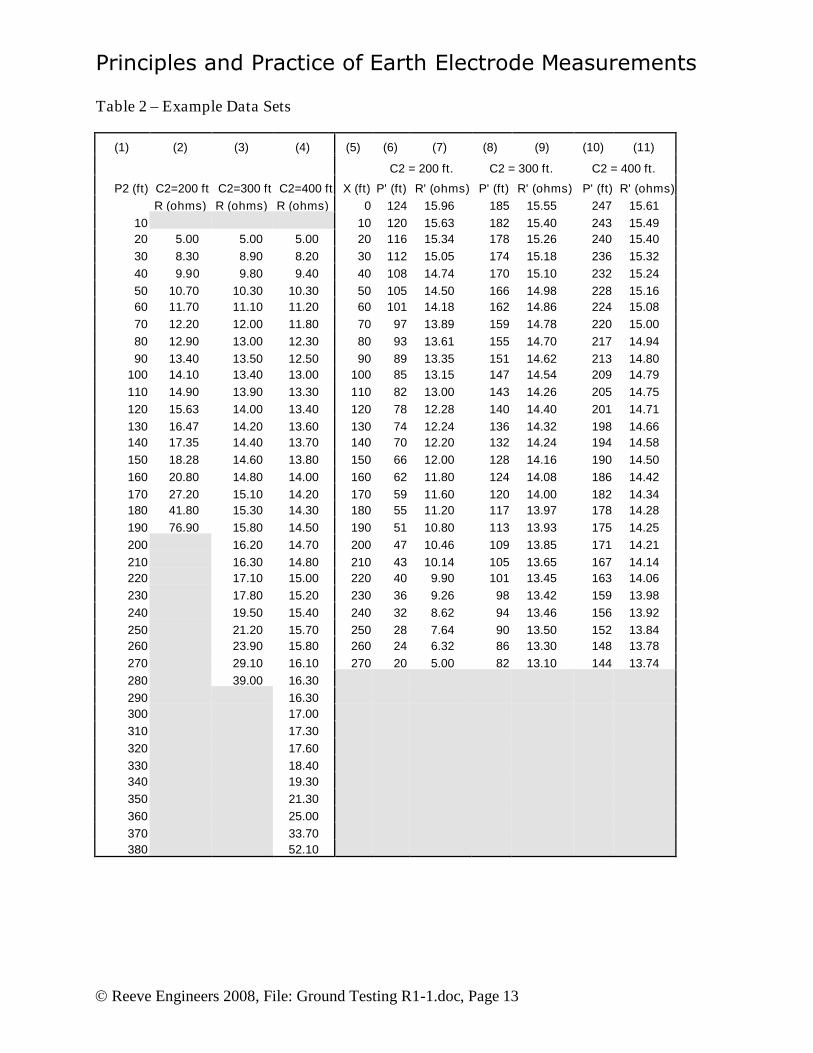
Example: The resistance data in Table 2 were measured at a site near Seward, AK. The earthelectrode consists of #2 AWG bare copper grid with overall dimensions of 40 feet by 60 feet.Grid spacing is 10 feet, and total conductor length is 580 feet. Burial depth is approximately 4feet below grade (underneath the building foundation).
Measurements in Columns (2), (3) and (4) were taken with the C2 probe at 200, 300 and 400 feetfrom the connection to the earth electrode. Columns (5) through (11) are for separateintersecting curve calculations that will be used in the next section.
The Fall-of-Potential curve corresponding to the measurements with C2 at 200 feet is fairlysteep, which indicates influence by the earth electrode (Fig. 9). The influence with C2 at 300
Principles and Practice of Earth Electrode Measurements
Reeve Engineers 2008, File: Ground Testing R1-1.doc, Page 12
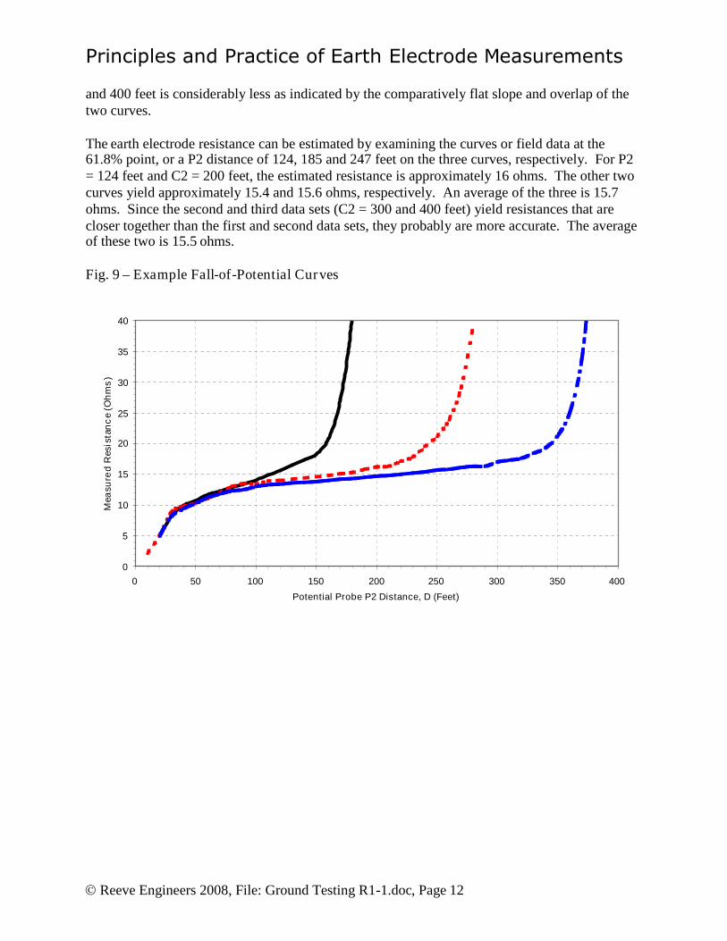
and 400 feet is considerably less as indicated by the comparatively flat slope and overlap of thetwo curves.
The earth electrode resistance can be estimated by examining the curves or field data at the61.8% point, or a P2 distance of 124, 185 and 247 feet on the three curves, respectively. For P2= 124 feet and C2 = 200 feet, the estimated resistance is approximately 16 ohms. The other twocurves yield approximately 15.4 and 15.6 ohms, respectively. An average of the three is 15.7ohms. Since the second and third data sets (C2 = 300 and 400 feet) yield resistances that arecloser together than the first and second data sets, they probably are more accurate. The averageof these two is 15.5 ohms.
Fig. 9 – Example Fall-of-Potential Curves
0
5
10
15
20
25
30
35
40
0 50 100 150 200 250 300 350 400
Potential Probe P2 Distance, D (Feet)
Mea
sure
dR
esis
tan
ce
(Oh
ms
)
Principles and Practice of Earth Electrode Measurements
Reeve Engineers 2008, File: Ground Testing R1-1.doc, Page 13
Table 2 – Example Data Sets
(1) (2) (3) (4) (5) (6) (7) (8) (9) (10) (11)
C2 = 200 ft. C2 = 300 ft. C2 = 400 ft.
P2 (ft) C2=200 ft C2=300 ft C2=400 ft X (ft) P' (ft) R' (ohms) P' (ft) R' (ohms) P' (ft) R' (ohms)R (ohms) R (ohms) R (ohms) 0 124 15.96 185 15.55 247 15.61
10 10 120 15.63 182 15.40 243 15.4920 5.00 5.00 5.00 20 116 15.34 178 15.26 240 15.4030 8.30 8.90 8.20 30 112 15.05 174 15.18 236 15.3240 9.90 9.80 9.40 40 108 14.74 170 15.10 232 15.2450 10.70 10.30 10.30 50 105 14.50 166 14.98 228 15.1660 11.70 11.10 11.20 60 101 14.18 162 14.86 224 15.0870 12.20 12.00 11.80 70 97 13.89 159 14.78 220 15.0080 12.90 13.00 12.30 80 93 13.61 155 14.70 217 14.9490 13.40 13.50 12.50 90 89 13.35 151 14.62 213 14.80
100 14.10 13.40 13.00 100 85 13.15 147 14.54 209 14.79110 14.90 13.90 13.30 110 82 13.00 143 14.26 205 14.75120 15.63 14.00 13.40 120 78 12.28 140 14.40 201 14.71130 16.47 14.20 13.60 130 74 12.24 136 14.32 198 14.66140 17.35 14.40 13.70 140 70 12.20 132 14.24 194 14.58150 18.28 14.60 13.80 150 66 12.00 128 14.16 190 14.50160 20.80 14.80 14.00 160 62 11.80 124 14.08 186 14.42170 27.20 15.10 14.20 170 59 11.60 120 14.00 182 14.34180 41.80 15.30 14.30 180 55 11.20 117 13.97 178 14.28190 76.90 15.80 14.50 190 51 10.80 113 13.93 175 14.25200 16.20 14.70 200 47 10.46 109 13.85 171 14.21210 16.30 14.80 210 43 10.14 105 13.65 167 14.14220 17.10 15.00 220 40 9.90 101 13.45 163 14.06230 17.80 15.20 230 36 9.26 98 13.42 159 13.98240 19.50 15.40 240 32 8.62 94 13.46 156 13.92250 21.20 15.70 250 28 7.64 90 13.50 152 13.84260 23.90 15.80 260 24 6.32 86 13.30 148 13.78270 29.10 16.10 270 20 5.00 82 13.10 144 13.74280 39.00 16.30290 16.30300 17.00310 17.30320 17.60330 18.40340 19.30350 21.30360 25.00370 33.70380 52.10
Principles and Practice of Earth Electrode Measurements
Reeve Engineers 2008, File: Ground Testing R1-1.doc, Page 14
5. Intersecting Curves Procedures
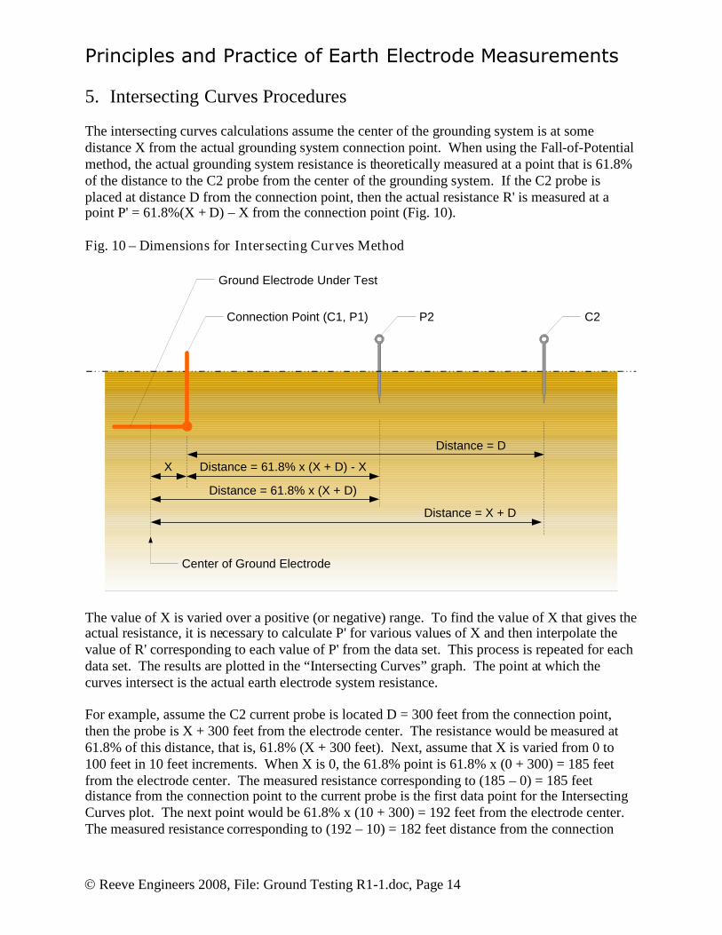
The intersecting curves calculations assume the center of the grounding system is at somedistance X from the actual grounding system connection point. When using the Fall-of-Potentialmethod, the actual grounding system resistance is theoretically measured at a point that is 61.8%of the distance to the C2 probe from the center of the grounding system. If the C2 probe isplaced at distance D from the connection point, then the actual resistance R' is measured at apoint P' = 61.8%(X + D) – X from the connection point (Fig. 10).
Fig. 10 – Dimensions for Intersecting Curves Method
Distance = 61.8% x (X + D) - X
Distance = D
Ground Electrode Under Test
Center of Ground Electrode
X
Distance = X + D
Connection Point (C1, P1)
Distance = 61.8% x (X + D)
P2 C2
The value of X is varied over a positive (or negative) range. To find the value of X that gives theactual resistance, it is necessary to calculate P' for various values of X and then interpolate thevalue of R' corresponding to each value of P' from the data set. This process is repeated for eachdata set. The results are plotted in the “Intersecting Curves” graph. The point at which thecurves intersect is the actual earth electrode system resistance.
For example, assume the C2 current probe is located D = 300 feet from the connection point,then the probe is X + 300 feet from the electrode center. The resistance would be measured at61.8% of this distance, that is, 61.8% (X + 300 feet). Next, assume that X is varied from 0 to100 feet in 10 feet increments. When X is 0, the 61.8% point is 61.8% x (0 + 300) = 185 feetfrom the electrode center. The measured resistance corresponding to (185 – 0) = 185 feetdistance from the connection point to the current probe is the first data point for the IntersectingCurves plot. The next point would be 61.8% x (10 + 300) = 192 feet from the electrode center.The measured resistance corresponding to (192 – 10) = 182 feet distance from the connection
Principles and Practice of Earth Electrode Measurements
Reeve Engineers 2008, File: Ground Testing R1-1.doc, Page 15
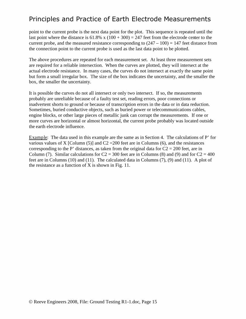
point to the current probe is the next data point for the plot. This sequence is repeated until thelast point where the distance is 61.8% x (100 + 300) = 247 feet from the electrode center to thecurrent probe, and the measured resistance corresponding to (247 – 100) = 147 feet distance fromthe connection point to the current probe is used as the last data point to be plotted.
The above procedures are repeated for each measurement set. At least three measurement setsare required for a reliable intersection. When the curves are plotted, they will intersect at theactual electrode resistance. In many cases, the curves do not intersect at exactly the same pointbut form a small irregular box. The size of the box indicates the uncertainty, and the smaller thebox, the smaller the uncertainty.
It is possible the curves do not all intersect or only two intersect. If so, the measurementsprobably are unreliable because of a faulty test set, reading errors, poor connections orinadvertent shorts to ground or because of transcription errors in the data or in data reduction.Sometimes, buried conductive objects, such as buried power or telecommunications cables,engine blocks, or other large pieces of metallic junk can corrupt the measurements. If one ormore curves are horizontal or almost horizontal, the current probe probably was located outsidethe earth electrode influence.
Example: The data used in this example are the same as in Section 4. The calculations of P’ forvarious values of X [Column (5)] and C2 =200 feet are in Columns (6), and the resistancescorresponding to the P’ distances, as taken from the original data for C2 = 200 feet, are inColumn (7). Similar calculations for C2 = 300 feet are in Columns (8) and (9) and for C2 = 400feet are in Columns (10) and (11). The calculated data in Columns (7), (9) and (11). A plot ofthe resistance as a function of X is shown in Fig. 11.
Principles and Practice of Earth Electrode Measurements
Reeve Engineers 2008, File: Ground Testing R1-1.doc, Page 16
Fig. 11 – Example Intersecting Curves
0
2
4
6
8
10
12
14
16
18
0 50 100 150 200 250 300 350
X Distance (Feet)
Res
ista
nc
e(O
hm
s)
Examination of the Intersecting Curves shows that the three curves cross at a resistance ofaround 15.5 ohms, which very closely agrees with the estimation made in Section 4. Thedistance X at the curve crossing is about 20 feet, indicating that the center of the earth electrodewas about 20 feet from the connection point as was actually the case.
6. Slope Procedures
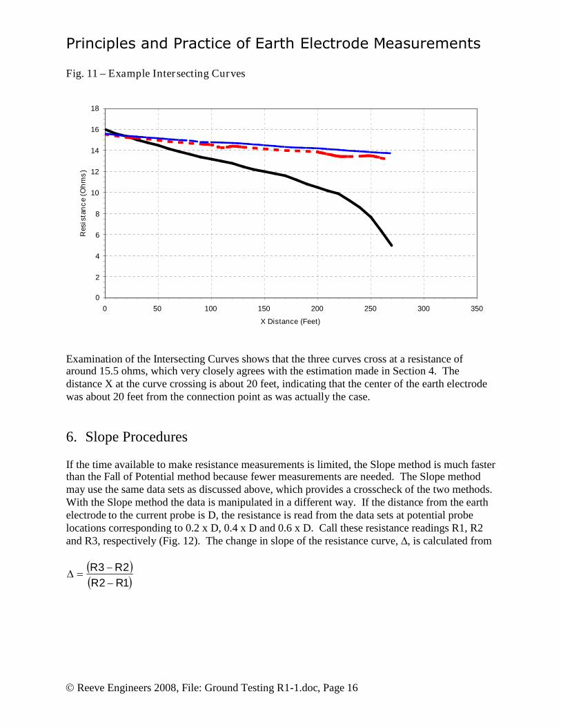
If the time available to make resistance measurements is limited, the Slope method is much fasterthan the Fall of Potential method because fewer measurements are needed. The Slope methodmay use the same data sets as discussed above, which provides a crosscheck of the two methods.With the Slope method the data is manipulated in a different way. If the distance from the earthelectrode to the current probe is D, the resistance is read from the data sets at potential probelocations corresponding to 0.2 x D, 0.4 x D and 0.6 x D. Call these resistance readings R1, R2and R3, respectively (Fig. 12). The change in slope of the resistance curve, , is calculated from
12
23RRRR
Principles and Practice of Earth Electrode Measurements
Reeve Engineers 2008, File: Ground Testing R1-1.doc, Page 17
Fig. 12 – Potential Probe P2 Locations for Slope Method
Distance = 0.2 x D
Distance = D
Ground Electrode Under Test
Center of Ground Electrode
Connection Point (C1, P1)
Distance = 0.6 x D
P2(R3)
C2
Distance = 0.4 x D
P2(R2)
P2(R1)
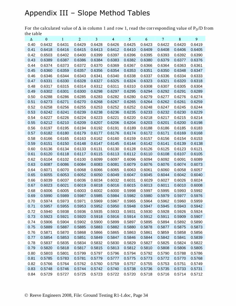
The table of values in Appendix III is then used to find the value ofDPD corresponding to the
calculated value of . If the calculated value of is not covered in the table, then the currentprobe is too close to the electrode system and additional measurements are required with agreater distance.
PD is the distance from the connection point to the potential probe where the true resistance
would be measured. PD is calculated by multiplying the quantityDPD (taken from the Slope
table) by the value D actually used. The resistance may then be found from the data set at thecalculated distance PD. If the data set does not include a measurement at the exact value of PD,the data may be interpolated, or a separate measurement can be made at the calculated value ofPD. A field data form is provided in Appendix IV for the Slope Method.
For example, assume that D = 300 feet and the calculated value of= 0.635. From the table in
Appendix II,DPD = 0.6079. Multiplying by D gives 0.6079 x 300 feet = 182 feet. This value
would be used to find the measured resistance from the original data with interpolation ifnecessary, or a resistance measurement would be made with the P2 probe at 182 feet.
Similar calculations should be made for each data set and the resulting resistances should agreewithin a few percent. The resistances so calculated can be plotted on a new graph with thedistance D on the horizontal scale (Fig. 11). Where the resistance significantly decreases as thedistance D increases (Data Set 1 and Data Set 2 in the example), the resistance values are higher
Principles and Practice of Earth Electrode Measurements
Reeve Engineers 2008, File: Ground Testing R1-1.doc, Page 18
than actual. Where the resistances are reasonably close (Data Set 2 and Data Set 3 in theexample), the values can be used with confidence.
Example: The data for this example is the same data that was used in Section 4. For C2 = 200feet, the 0.2 xD = 40 feet, 0.4 x D = 80 feet and 0.6 x D = 120 feet. The correspondingresistances from the original data at these distances are R1 = 9.90 ohms, R2 = 12.30 ohms, andR3 = 15.63 ohms.
Calculating for this data set gives 12
23
RR
RR
= 1.388.
From Appendix II, PD/D = 0.4350. Since D = 200 feet, PD = 0.4350 x 200 feet = 87 feet. Themeasured resistance corresponding to P2 distance of 87 feet, as interpolated from the originalmeasurements for C2 = 200 feet, is approximately 15.1 ohms.
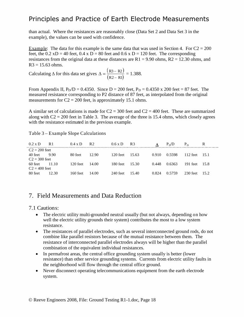
A similar set of calculations is made for C2 = 300 feet and C2 = 400 feet. These are summarizedalong with C2 = 200 feet in Table 3. The average of the three is 15.4 ohms, which closely agreeswith the resistance estimated in the previous example.
Table 3 – Example Slope Calculations
0.2 x D R1 0.4 x D R2 0.6 x D R3 PD/D PD RC2 = 200 feet40 feet 9.90 80 feet 12.90 120 feet 15.63 0.910 0.5598 112 feet 15.1C2 = 300 feet60 feet 11.10 120 feet 14.00 180 feet 15.30 0.448 0.6363 191 feet 15.8C2 = 400 feet80 feet 12.30 160 feet 14.00 240 feet 15.40 0.824 0.5759 230 feet 15.2
7. Field Measurements and Data Reduction
7.1 Cautions: The electric utility multi-grounded neutral usually (but not always, depending on how
well the electric utility grounds their system) contributes the most to a low systemresistance.
The resistances of parallel electrodes, such as several interconnected ground rods, do notcombine like parallel resistors because of the mutual resistance between them. Theresistance of interconnected parallel electrodes always will be higher than the parallelcombination of the equivalent individual resistances.
In permafrost areas, the central office grounding system usually is better (lowerresistance) than other service grounding systems. Currents from electric utility faults inthe neighborhood will flow through the central office ground.
Never disconnect operating telecommunications equipment from the earth electrodesystem.

Principles and Practice of Earth Electrode Measurements
Reeve Engineers 2008, File: Ground Testing R1-1.doc, Page 19
Never disconnect live ac service equipment from the earth electrode system – this is foryour safety.
In a new central office, with no live equipment and no live ac service, it will be possibleto test individual grounding system components (well casing, grid, ground rods, buildingstructural steel, etc.) if they can be isolated from each other. Otherwise, leave everythinginterconnected and measure the overall system.
Usually, telecommunications facility earth electrode systems consist of severalcomponents and the facility operates normally with all the components interconnected.Therefore, if your goal is to measure only the telecommunications facility earth electrodesystem, you would not measure them individually. Instead, you would make sure allcomponents, except the electric utility MGN, are bonded as they would be in the finaloperating configuration and measure them as a complete system.
If you leave all earth electrode components interconnected for safety, you are measuringthe composite resistance of all earth electrode components together, including the electricutility multi-grounded neutral (MGN). Usually, the electric utility MGN will contributethe most to a low resistance reading. Remember: This kind of test (with everythinginterconnected, including the electric utility MGN) will not yield valid results if your goalis to measure only the building or enclosure earth electrode system.
If you can safely disconnect an individual electrode component from the groundingelectrode system, then you can correctly measure that component.
Frozen ground is an insulator. Readings taken during the summer when the active soillayer is thawed are meaningless for winter. Where the winter frost depth exceeds thedepth of earth electrodes, the electrodes are insulated from remote earth and theresistance of the electrode system will be very high. To reduce potential differences forsafety and operation, all metallic components of the telecommunications facility must bebonded together.
7.2 Test Instruments: Battery operated test sets with an analog null meter are the best, provide the most
consistent measurements and are the most reliable. The hand-crank test set by Biddle and other manufacturers works fine but are relatively
difficult and awkward to use. Some digital test sets most often do not yield usable data. This is particularly the case if
the earth electrode system being measured is near a power plant or substation. Always test your test set before taking it into the field. The manual tells you how to do
this. Take an extra set of batteries. If the test set uses rechargeable batteries, make sure they
are not worn out and have enough charge for the measurements to be made. Occasionally check calibration especially if the test set has not been taken care of in the
field or in storage or if it has been in storage for a long time. The manual tells you howto do this (you will need some resistors).
For earth electrode measurements, always short the P1 and C1 terminals together or useseparate test leads, one from P1 to the earth electrode and one from C1 to the earthelectrode. The latter provides the best accuracy.
Principles and Practice of Earth Electrode Measurements
Reeve Engineers 2008, File: Ground Testing R1-1.doc, Page 20
7.3 Test Leads – General Information: Use a heavy-gauge (14 - 16 AWG) test lead wire and lots of it. The lead connected to the current probe (C2) should have a total overall length of 300-
400 ft or more The lead connected to the potential probe (P2) should have a total overall length of 300-
400 ft or more (it should have the same overall length as the C2 lead) The lead connected from C1/P1 to the grounding electrode system should be as short as
possible, preferably less than 10 ft long. If this lead is too long, the readings will not bereliable. The resistance of this lead directly affects the measured resistance. One way toeliminate this measurement error is to use a separate lead from the C1 terminal to thegrounding electrode system and a separate lead from the P1 terminal to the groundingelectrode.
7.4 Test Lead Kit: You will need approximately 600 ft – 800 ft of test lead wire (300 ft – 400 ft for P2 and
300 ft – 400 ft for C2). Make up two test leads, each 100 ft long, with a large (2 in. or 3 in.) alligator clip at one
end and 1/4 in. fork terminal lug at the other. One will connect to the C2 terminal and theother to the P2 terminal on the test set. Use rubber insulating boots over the alligatorclips
Use the remaining test lead wire to make 100 ft sections with large insulated alligatorclips at each end.
Make up one test lead, 10 ft long, with large alligator clip at one end and 1/4 in. forkterminal lug at the other. This will be used to connect P1/C1 terminal on the test set tothe grounding electrode system. Also make up extra test leads if it is necessary to locatethe test set some distance from the connection point at the earth electrode (one test leadfor C1 and one for P1).
Put test leads on 12 in. or 14 in. “Cordwheels.” These are available from hardware stores(Home Depot, Lowes) and are designed for coiling extension cords but work well withtest leads.
Put spare terminal lugs and alligator clips in the kit along with a crimping tool,screwdriver and any other tools you may need to repair the test leads in the field. Be sureto include a set of good gloves.
The test lead kit also should include safety glasses, gloves, and a short-handle, 4 lb.,double-head hammer, and test probes (see below).
7.5 Test Leads – Connections: When stringing out the test leads, make sure the insulation is not damaged. Use gloves to
handle the wire, especially if the leads are strung below or above power lines. Where test lead sections are connected together to make a longer lead, be sure to insulate
the alligator clips from the earth and foliage. Use 8 in. lengths of 1-1/2 in. or 2 in.flexible non-metallic conduit or other insulating material as insulator sleeves (these areslipped over the alligator clips to keep them from touching the ground).
Be sure to clean the point of connection to the grounding electrode system. UseScotchBrite or wire brush.

Principles and Practice of Earth Electrode Measurements
Reeve Engineers 2008, File: Ground Testing R1-1.doc, Page 21
The farther the current probe (C2) is from the grounding electrode system, the better.The object is to get the P2 probe out of the influence of the grounding electrode systemwhen P2 is 61.8% of the distance to C2. If the largest dimension of the electrode systemis x ft, the C2 probe should be 10x ft to 20x ft from the electrode system. For example, ifthe grounding electrode is 20 ft x 20 ft, C2 should be at least 200 ft to 400 ft away.Unfortunately, the extent of the grounding system usually is unknown, so you will try toplace the C2 probe as far away as possible. To calculate resistance, you almost alwayswill have to use the “Intersecting Curves” or the “Slope” method..
Never disconnect the ac service equipment from the earth electrode system. Neverdisconnect working telecommunications equipment from ground. In a new central office,with no live equipment and no live ac service, it will be possible to test individualgrounding system components (well casing, grid, ground rods, building structural steel,etc.) if they can be isolated from each other. Otherwise, leave everything interconnectedand measure the overall system – this is for your safety.
7.6 Test Probes: Test probes should be 18 – 20 in. long and made from strong galvanized steel. They
should have a loop at one end and sharpened to a point at the other. Purchase ready-madeprobes from Biddle (Fig. 15) or make your own but carry extras.
It is a good idea to carry a couple longer probes made from a cut ground rod, 3 ft – 4 ftlong, for use where the shorter probes do not make good enough contact with the earth.Weld a T-bar near the top of these longer rods so you can twist and pull them out of theground.
The probes normally only have to be driven to a depth of 6 in. – 12. in. The deeper theprobe the harder it is to pull out. Wear safety glasses when driving the probes.
Remove probes by twisting and pulling on the loop at the top of the probe; do not hit theside of the probe with a hammer or kick it to loosen it because all you will do is bend theprobe and ruin it.
If you have to place the probes in a parking area or roadway with very hard ground,concrete or pavement, use metal plates in place of the pointed probes. Lay the plates onthe ground and wet them and the area around them thoroughly. An alternative is to drillthrough the pavement or concrete with a hammer drill.
Be sure the alligator clip makes a good connection where it is connected to the probe.Use 3M ScotchBrite or wire brush to clean the probes where you connect the alligatorclips.
P2 should be placed in a straight line between the connection point and C2. Sometimes itwill be necessary to place C2 in one direction but move in another direction with P2,although some test set manufacturers recommend against this procedure. If you do this,move P2 in a straight line away from the connection point and away from the electrodesystem.
Avoid placing the probes in line with underground facilities (electric, telephone, metallicwater and sewer pipes, etc.) but sometimes you have no choice.
Be aware of shallow underground facilities, such as telephone cables, when you drive theprobes.
Principles and Practice of Earth Electrode Measurements
Reeve Engineers 2008, File: Ground Testing R1-1.doc, Page 22
7.7 Readings: Start your readings with the P2 probe 10 ft – 20 ft from the point of connection. Take a reading every 10 ft to within 20 ft – 30 ft of C2. You will notice the readings are
low when you are close to the point of connection and slowly climb. If C2 is far enoughaway, the readings will level off in the middle. As you approach C2, the readings climbrapidly.
If C2 is far from the influence of the electrode system, the readings will level off near the61.8% point. When P2 is closer to the connection point, the readings will be lower andwhen closer to C2, the readings will be higher. Readings that decrease as you move awayfrom the connection point indicate underground metallic facilities that are interferingwith the measurements or that the P2 probe is over the grounding electrode. Anoccasional dip in the readings is not unusual, but if several readings follow this pattern,you have to move C2 and start over.
Always take at least three separate sets of readings. Usually, you can take two sets ofreadings with the C2 probe at two different distances along the same direction, say 300 ftand 250 ft, although 400 ft and 300 ft are preferable. Take the third set of readings inanother direction if possible. Depending on the topography and obstructions, you mayhave to take all three readings in the same direction (say, 400 ft, 300 ft and 200 ft or 300ft, 250 ft and 200 ft).
If you are able to move the test set analog meter needle to either side of null (with theresistance knobs), the probes are deep enough. If the needle moves only to one side(usually the “ – “ side), one or both probes are not deep enough, you have a badconnection, or the alligator clips used to splice lead sections are in contact with the earth.Check all connections and try driving the probes a little deeper or use the longer probes.You also can try pouring water around the probe. In any case, you must be able to movethe needle to both sides of null with the resistance knobs; otherwise, the reading is notreliable.
With analog instruments, the null sometimes will be lazy (move slowly as you adjust theresistance knobs), which indicates underground metallic facilities or inadequate probecontact. For the latter situation, drive the probes deeper or use longer probes.
With analog instruments, the meter sometimes will oscillate around null. You will haveto adjust the resistance knobs so the meter moves an equal distance left and right of null(center) and then take a reading; this takes practice and a little practice.
Digital instruments include fault indicators that indicate excessively high probe resistanceor bad connections. If you see this indication, check all connections and, if necessary,drive the probes deeper.
7.8 Data Reduction: The actual electrode system resistance is measured when P2 is 61.8% of the distance C2
is from the center of the electrode system. However, the actual center of the electrodesystem seldom is known except in small systems, so the location of this 61.8% point isnever known accurately. A small system would be a few ground rods that are notconnected to anything else other than each other.
If measuring a small system, you can put C2 outside the influence (10X – 20X asmentioned above) and then put P2 at a point 61.8% of this distance. The reading youtake at this point will be close to the actual electrode system resistance. Additional

Principles and Practice of Earth Electrode Measurements
Reeve Engineers 2008, File: Ground Testing R1-1.doc, Page 23
readings are not necessary, but they should be taken anyway to ensure that the data isvalid.
If measuring larger systems, you should use the “Intersecting Curves” or “Slope” method.
Fig. 15 - T-Handle, Factory-Made Test Probes in a kit of four
8. Soil Resistivity Measurements
Soil resistivity is a measure of how well the soil passes electrical current. Soil with highresistivity does not pass current well. Resistivity is defined in terms of the electrical resistanceof a cube of soil. The resistance of this cube, as measured across its faces, is proportional to theresistivity and inversely proportional to the length of one side of the cube.
The resistivity of the soil in which the earth electrode is buried is the limiting factor in attaininglow electrode resistance. Soil with low resistivity is better for building low resistance earthelectrodes than soil with high resistivity. Soil resistivity depends on soil type, salt concentration,moisture content and temperature.
Formulas for specific electrode configurations are available in reference handbooks. Therefore,if the soil resistivity is known, the resistance of many common earth electrode configurations canbe readily calculated. These formulas are beyond the scope of the present article.1 From anoperational standpoint, soil resistivity measurements allow for initial earth electrode designbased on these formulas and in prediction of the effects of changes to an existing electrode.
The resistivities of various soil types are given in Table 4. A wide range of soil types may befound in any given area or the soil types may vary widely with depth, or both. The season andweather conditions will greatly affect the soil resistivity. For example, high resistivity rock canbe overlain by clays that have low resistivity in the summer but have high resistivities in thewinter when frozen.
1 See, for example, MIL-HDBK-419a, Grounding, Bonding, and Shielding for Electronic Equipments and Facilitiesand Rural Utilities Service Bulletin 1751F-802, Electrical Protection Grounding Fundamentals.
Principles and Practice of Earth Electrode Measurements
Reeve Engineers 2008, File: Ground Testing R1-1.doc, Page 24
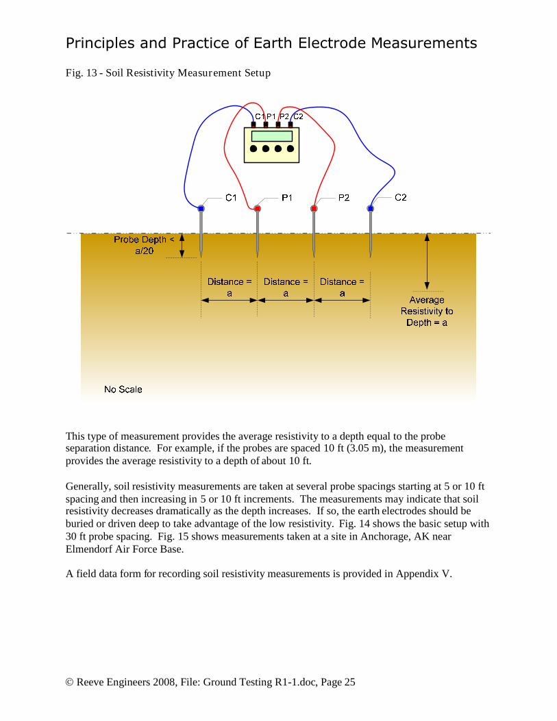
Resistivity measurements provide an average reading. The method almost always used anddescribed here assumes the soil is homogeneous (all the same or similar kind). Soil resistivity ismeasured by injecting a current into the earth, measuring the voltage drop, and then calculatingthe resistance. Four-terminal test sets do the resistance calculations automatically. If the fourprobes are placed equidistance from each other and in a straight line as shown in Fig. 13, theresistivity can be calculated from (for separation measured in ft)
Ra ft 915.1 ohm-m
where = Soil resistivity, ohm-ma = Distance between the four equally spaced probes, ftR = Measured resistance, ohms
or (for separation measured in m)
Ram 283.6 ohm-m
where = Soil resistivity, ohm-ma = Distance between each of the four equally spaced probes, mR = Measured resistance, ohms
Be careful with units of measurement and be sure to use the correct formula. Most soilresistivity tables are in units of ohm-m or ohm-cm but most distance or length measurements inthe United States are (unfortunately) in ft.
The above formulas are valid only if the probes are buried no more than 1/20 of the separationdistance, a. For example, if the probes are spaced 5 ft (1.5 m), they cannot be driven more thanabout 3 in. (0.075 m). Every effort should be made to drive all four probes to the same depth.
Principles and Practice of Earth Electrode Measurements
Reeve Engineers 2008, File: Ground Testing R1-1.doc, Page 25
Fig. 13 - Soil Resistivity Measurement Setup
This type of measurement provides the average resistivity to a depth equal to the probeseparation distance. For example, if the probes are spaced 10 ft (3.05 m), the measurementprovides the average resistivity to a depth of about 10 ft.
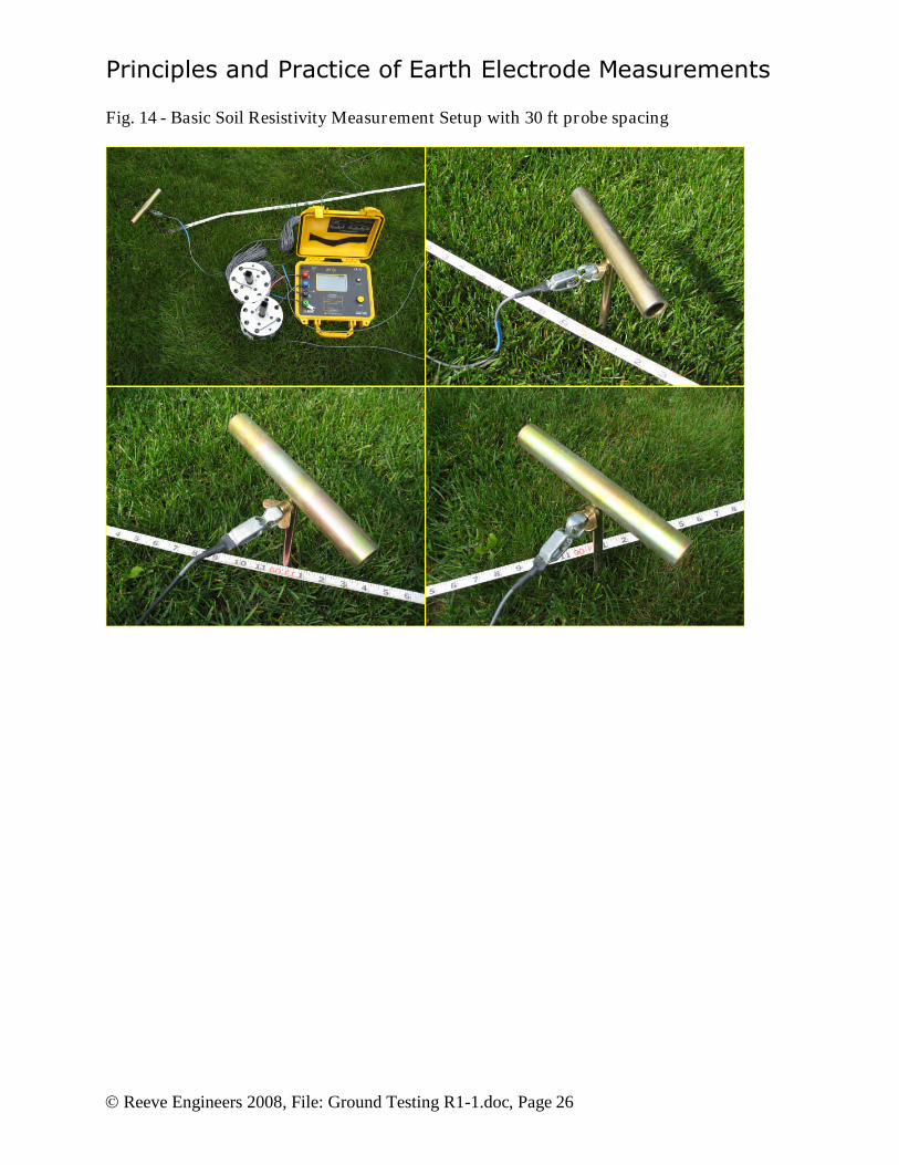
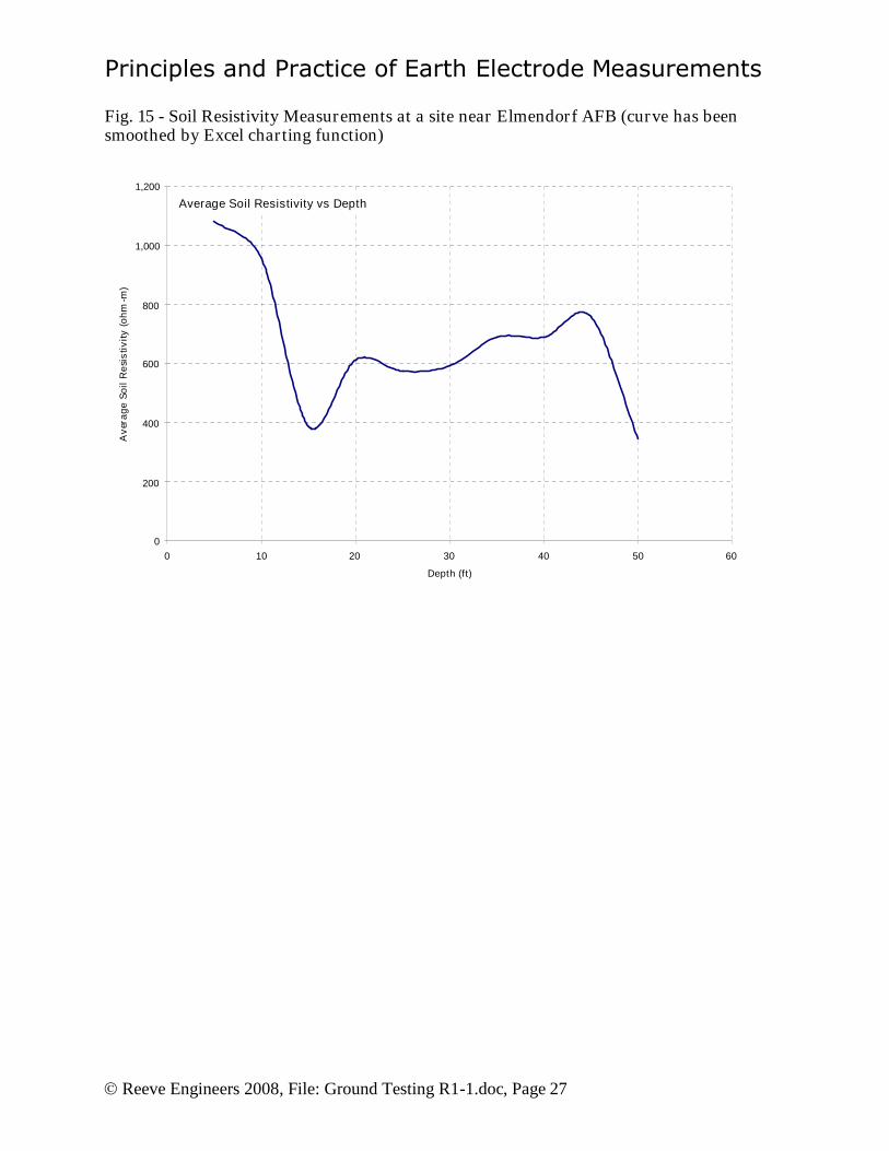
Generally, soil resistivity measurements are taken at several probe spacings starting at 5 or 10 ftspacing and then increasing in 5 or 10 ft increments. The measurements may indicate that soilresistivity decreases dramatically as the depth increases. If so, the earth electrodes should beburied or driven deep to take advantage of the low resistivity. Fig. 14 shows the basic setup with30 ft probe spacing. Fig. 15 shows measurements taken at a site in Anchorage, AK nearElmendorf Air Force Base.
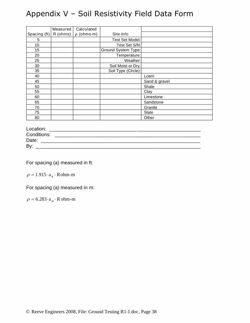
A field data form for recording soil resistivity measurements is provided in Appendix V.
Principles and Practice of Earth Electrode Measurements
Reeve Engineers 2008, File: Ground Testing R1-1.doc, Page 26
Fig. 14 - Basic Soil Resistivity Measurement Setup with 30 ft probe spacing
Principles and Practice of Earth Electrode Measurements
Reeve Engineers 2008, File: Ground Testing R1-1.doc, Page 27
Fig. 15 - Soil Resistivity Measurements at a site near Elmendorf AFB (curve has beensmoothed by Excel charting function)
Average Soil Resistivity vs Depth
0
200
400
600
800
1,000
1,200
0 10 20 30 40 50 60
Depth (ft)
Ave
rage
Soil
Res
istiv
ity(o
hm-m
)
Principles and Practice of Earth Electrode Measurements
Reeve Engineers 2008, File: Ground Testing R1-1.doc, Page 28
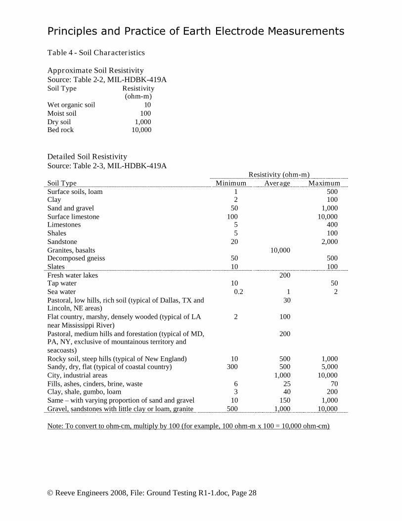
Table 4 - Soil Characteristics
Approximate Soil ResistivitySource: Table 2-2, MIL-HDBK-419ASoil Type Resistivity
(ohm-m)Wet organic soil 10Moist soil 100Dry soil 1,000Bed rock 10,000
Detailed Soil ResistivitySource: Table 2-3, MIL-HDBK-419A
Soil TypeResistivity (ohm-m)
Minimum Average MaximumSurface soils, loam 1 500Clay 2 100Sand and gravel 50 1,000Surface limestone 100 10,000Limestones 5 400Shales 5 100Sandstone 20 2,000Granites, basalts 10,000Decomposed gneiss 50 500Slates 10 100Fresh water lakes 200Tap water 10 50Sea water 0.2 1 2Pastoral, low hills, rich soil (typical of Dallas, TX andLincoln, NE areas)
30
Flat country, marshy, densely wooded (typical of LAnear Mississippi River)
2 100
Pastoral, medium hills and forestation (typical of MD,PA, NY, exclusive of mountainous territory andseacoasts)
200
Rocky soil, steep hills (typical of New England) 10 500 1,000Sandy, dry, flat (typical of coastal country) 300 500 5,000City, industrial areas 1,000 10,000Fills, ashes, cinders, brine, waste 6 25 70Clay, shale, gumbo, loam 3 40 200Same – with varying proportion of sand and gravel 10 150 1,000Gravel, sandstones with little clay or loam, granite 500 1,000 10,000
Note: To convert to ohm-cm, multiply by 100 (for example, 100 ohm-m x 100 = 10,000 ohm-cm)

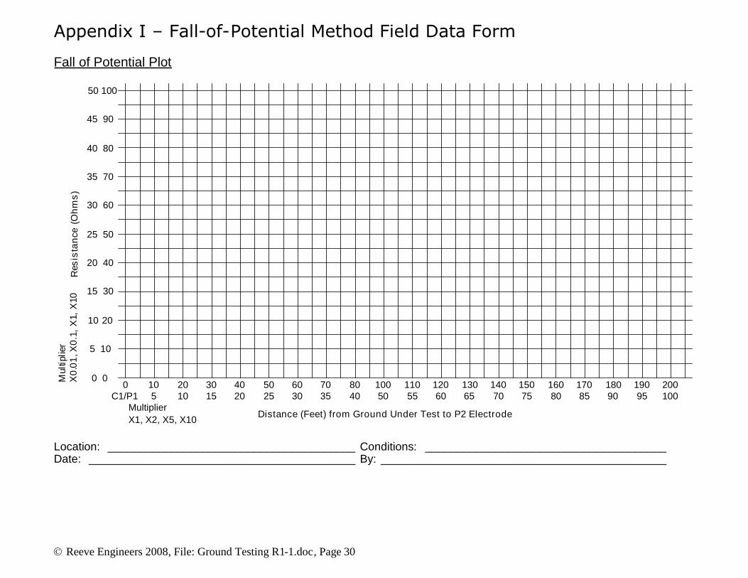
Appendix I – Fall-of-Potential Method Field Data Form
Reeve Engineers 2008, File: Ground Testing R1-1.doc, Page 29
Place the C2 probe as far as possible from the ground under test (typically 200,300 and 400 ft.). Place the P2 probe at 10 or 20 ft. intervals in a straight linewith C2. Measure and record the resistance reading on the test set.
P2 (ft) R (ohms) R (ohms) R (ohms) Site Info0 C2 = C2 = C2 = Test Set Model:
10 Test Set S/N:20 Ground System Type:30 Temperature:40 Weather:50 Soil Moist or Dry:60 Soil Type (Circle):70 Loam80 Sand & gravel90 Shale
100 Clay110 Limestone120 Sandstone130 Granite140 Slate150 Other160170180190 Notes:200210220230240250260270280290300310320330340350360370380390
Location: _______________________________________________________Conditions: ______________________________________________________Date: __________________________________________________________By: ____________________________________________________________
Appendix I – Fall-of-Potential Method Field Data Form
Reeve Engineers 2008, File: Ground Testing R1-1.doc, Page 30
Fall of Potential Plot
0C1/P1
105
2010
3015
4020
5025
6030
7035
8040
10050
11055
12060
13065
14070
15075
16080
17085
18090
19095
200100
MultiplierX1, X2, X5, X10 Distance (Feet) from Ground Under Test to P2 Electrode
5 10
0 0
10 20
15 30
20 40
25 50
30 60
35 70
40 80
45 90
50 100
Res
ista
nce
(Ohm
s)M
ultip
lier
X0.
01,X
0.1,
X1,
X10
Location: _______________________________________ Conditions: ______________________________________Date: __________________________________________ By: _____________________________________________
Appendix II – Derivation of Measurement Points
Reeve Engineers 2008, File: Ground Testing R1-1.doc, Page 31
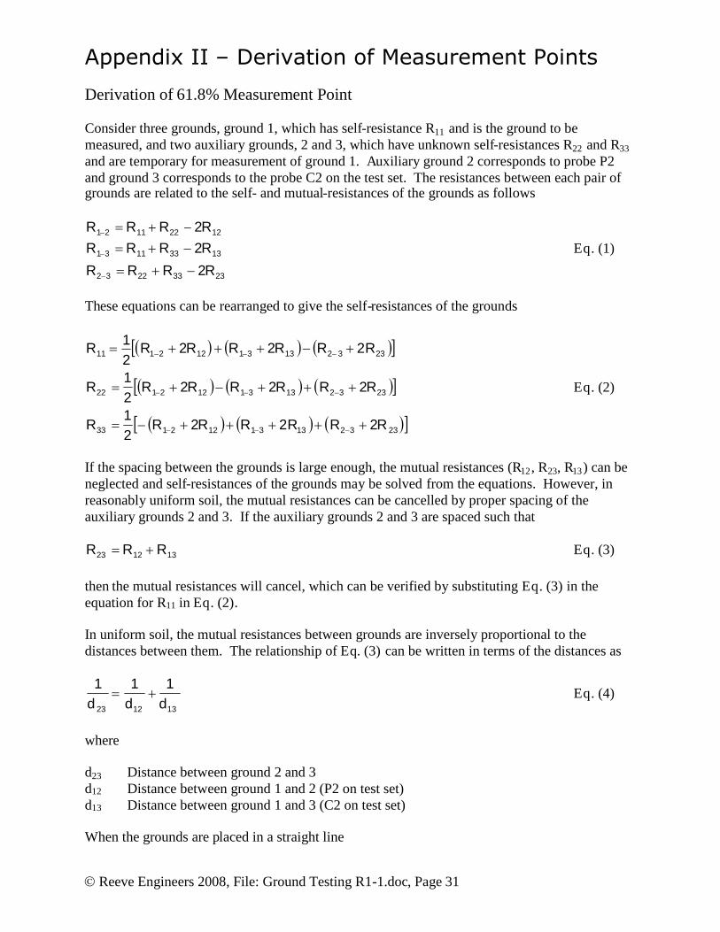
Derivation of 61.8% Measurement Point
Consider three grounds, ground 1, which has self-resistance R11 and is the ground to bemeasured, and two auxiliary grounds, 2 and 3, which have unknown self-resistances R22 and R33and are temporary for measurement of ground 1. Auxiliary ground 2 corresponds to probe P2and ground 3 corresponds to the probe C2 on the test set. The resistances between each pair ofgrounds are related to the self- and mutual-resistances of the grounds as follows
23332232
13331131
12221121
2
22
RRRR
RRRRRRRR
Eq. (1)
These equations can be rearranged to give the self-resistances of the grounds
23321331122133
23321331122122
23321331122111
22221
22221
22221
RRRRRRR
RRRRRRR
RRRRRRR
Eq. (2)
If the spacing between the grounds is large enough, the mutual resistances (R12 , R23, R13) can beneglected and self-resistances of the grounds may be solved from the equations. However, inreasonably uniform soil, the mutual resistances can be cancelled by proper spacing of theauxiliary grounds 2 and 3. If the auxiliary grounds 2 and 3 are spaced such that
131223 RRR Eq. (3)
then the mutual resistances will cancel, which can be verified by substituting Eq. (3) in theequation for R11 in Eq. (2).
In uniform soil, the mutual resistances between grounds are inversely proportional to thedistances between them. The relationship of Eq. (3) can be written in terms of the distances as
131223
111ddd
Eq. (4)
where
d23 Distance between ground 2 and 3d12 Distance between ground 1 and 2 (P2 on test set)d13 Distance between ground 1 and 3 (C2 on test set)
When the grounds are placed in a straight line
Appendix II – Derivation of Measurement Points
Reeve Engineers 2008, File: Ground Testing R1-1.doc, Page 32
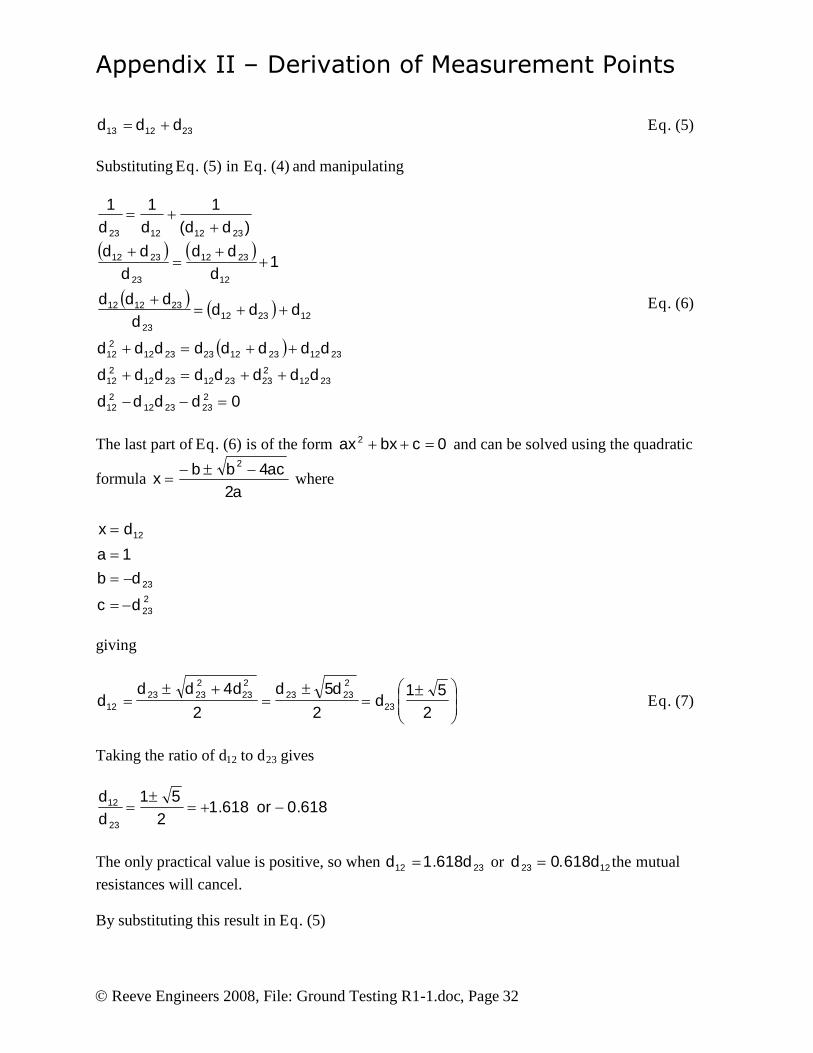
231213 ddd Eq. (5)
Substituting Eq. (5) in Eq. (4) and manipulating
0
1
)(111
2232312
212
231222323122312
212
231223122323122
12
12231223
231212
12
2312
23
2312
23121223
dddd
dddddddd
dddddddd
dddd
ddd
ddd
ddd
dddd
Eq. (6)
The last part of Eq. (6) is of the form 02 cbxax and can be solved using the quadratic
formulaa
acbbx2
42 where
223
23
12
1
dc
dba
dx
giving
251
25
24
23
22323
223
22323
12 dddddd
d Eq. (7)
Taking the ratio of d12 to d23 gives
618.0or618.12
51
23
12
dd
The only practical value is positive, so when 2312 618.1 dd or 1223 618.0 dd the mutualresistances will cancel.
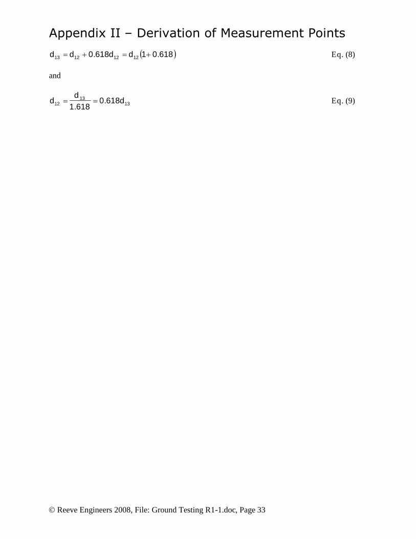
By substituting this result in Eq. (5)
Appendix II – Derivation of Measurement Points
Reeve Engineers 2008, File: Ground Testing R1-1.doc, Page 33
618.01618.0 12121213 dddd Eq. (8)
and
1313
12 618.0618.1
dd
d Eq. (9)
Appendix III – Slope Method Tables
Reeve Engineers 2008, File: Ground Testing R1-1.doc, Page 34
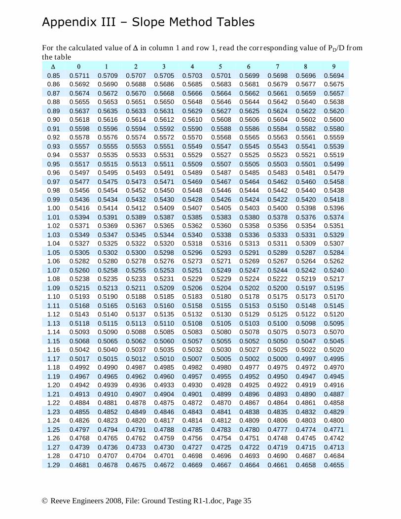
For the calculated value of in column 1 and row 1, read the corresponding value of PD/D fromthe table
0.40 0.6432 0.6431 0.6429 0.6428 0.6426 0.6425 0.6423 0.6422 0.6420 0.64190.41 0.6418 0.6416 0.6415 0.6413 0.6412 0.6410 0.6409 0.6408 0.6406 0.64050.42 0.6503 0.6402 0.6400 0.6399 0.6397 0.6396 0.6395 0.6393 0.6392 0.63900.43 0.6389 0.6387 0.6386 0.6384 0.6383 0.6382 0.6380 0.6379 0.6377 0.63760.44 0.6374 0.6373 0.6372 0.6370 0.6369 0.6367 0.6366 0.6364 0.6363 0.63610.45 0.6360 0.6359 0.6357 0.6356 0.6354 0.6353 0.6351 0.6350 0.6348 0.63470.46 0.6346 0.6344 0.6343 0.6341 0.6340 0.6338 0.6337 0.6336 0.6334 0.63330.47 0.6331 0.6330 0.6328 0.6327 0.6325 0.6324 0.6323 0.6321 0.6320 0.63180.48 0.6317 0.6315 0.6314 0.6312 0.6311 0.6310 0.6308 0.6307 0.6305 0.63040.49 0.6302 0.6301 0.6300 0.6298 0.6297 0.6295 0.6294 0.6292 0.6291 0.62890.50 0.6288 0.6286 0.6285 0.6283 0.6282 0.6280 0.6279 0.6277 0.6276 0.62740.51 0.6273 0.6271 0.6270 0.6268 0.6267 0.6265 0.6264 0.6262 0.6261 0.62590.52 0.6258 0.6256 0.6255 0.6253 0.6252 0.6252 0.6248 0.6247 0.6245 0.62440.53 0.6242 0.6241 0.6239 0.6238 0.6236 0.6235 0.6233 0.6232 0.6230 0.62290.54 0.6227 0.6226 0.6224 0.6223 0.6221 0.6220 0.6218 0.6217 0.6215 0.62140.55 0.6212 0.6210 0.6209 0.6207 0.6206 0.6204 0.6203 0.6201 0.6200 0.61980.56 0.6197 0.6195 0.6194 0.6192 0.6191 0.6189 0.6188 0.6186 0.6185 0.61830.57 0.6182 0.6180 0.6179 0.6177 0.6176 0.6174 0.6172 0.6171 0.6169 0.61680.58 0.6166 0.6165 0.6163 0.6162 0.6160 0.6159 0.6157 0.6156 0.6154 0.61530.59 0.6151 0.6150 0.6148 0.6147 0.6145 0.6144 0.6142 0.6141 0.6139 0.61380.60 0.6136 0.6134 0.6133 0.6131 0.6130 0.6128 0.6126 0.6125 0.6123 0.61210.61 0.6120 0.6118 0.6117 0.6115 0.6113 0.6112 0.6110 0.6108 0.6107 0.61050.62 0.6104 0.6102 0.6100 0.6099 0.6097 0.6096 0.6094 0.6092 0.6091 0.60890.63 0.6087 0.6086 0.6084 0.6083 0.6081 0.6079 0.6076 0.6076 0.6074 0.60730.64 0.6071 0.6070 0.6068 0.6066 0.6065 0.6063 0.6061 0.6060 0.6058 0.60570.65 0.6055 0.6053 0.6052 0.6050 0.6049 0.6047 0.6045 0.6044 0.6042 0.60400.66 0.6039 0.6037 0.6036 0.6034 0.6032 0.6031 0.6029 0.6027 0.6026 0.60240.67 0.6023 0.6021 0.6019 0.6018 0.6016 0.6015 0.6013 0.6011 0.6010 0.60080.68 0.6006 0.6005 0.6003 0.6002 0.6000 0.5998 0.5997 0.5995 0.5993 0.59920.69 0.5990 0.5989 0.5987 0.5985 0.5984 0.5982 0.5980 0.5979 0.5977 0.59760.70 0.5974 0.5973 0.5971 0.5969 0.5967 0.5965 0.5964 0.5962 0.5960 0.59590.71 0.5957 0.5955 0.5953 0.5952 0.5950 0.5948 0.5947 0.5945 0.5943 0.59420.72 0.5940 0.5938 0.5936 0.5935 0.5933 0.5931 0.5930 0.5928 0.5926 0.59240.73 0.5923 0.5921 0.5920 0.5918 0.5916 0.5914 0.5912 0.5911 0.5909 0.59070.74 0.5906 0.5904 0.5902 0.5900 0.5899 0.5897 0.5895 0.5894 0.5892 0.58900.75 0.5889 0.5887 0.5885 0.5883 0.5882 0.5880 0.5878 0.5877 0.5875 0.58730.76 0.5871 0.5870 0.5868 0.5866 0.5865 0.5863 0.5861 0.5859 0.5858 0.58560.77 0.5854 0.5853 0.5851 0.5849 0.5847 0.5846 0.5844 0.5842 0.5841 0.58390.78 0.5837 0.5835 0.5834 0.5832 0.5830 0.5829 0.5827 0.5825 0.5824 0.58220.79 0.5820 0.5818 0.5817 0.5815 0.5813 0.5812 0.5810 0.5808 0.5806 0.58050.80 0.5803 0.5801 0.5799 0.5797 0.5796 0.5794 0.5792 0.5790 0.5788 0.57860.81 0.5785 0.5783 0.5781 0.5779 0.5777 0.5775 0.5773 0.5772 0.5770 0.57680.82 0.5766 0.5764 0.5762 0.5760 0.5759 0.5757 0.5755 0.5753 0.5751 0.57490.83 0.5748 0.5746 0.5744 0.5742 0.5740 0.5738 0.5736 0.5735 0.5733 0.57310.84 0.5729 0.5727 0.5725 0.5723 0.5722 0.5720 0.5718 0.5716 0.5714 0.5712
Appendix III – Slope Method Tables
Reeve Engineers 2008, File: Ground Testing R1-1.doc, Page 35
For the calculated value of in column 1 and row 1, read the corresponding value of PD/D fromthe table
0.85 0.5711 0.5709 0.5707 0.5705 0.5703 0.5701 0.5699 0.5698 0.5696 0.56940.86 0.5692 0.5690 0.5688 0.5686 0.5685 0.5683 0.5681 0.5679 0.5677 0.56750.87 0.5674 0.5672 0.5670 0.5668 0.5666 0.5664 0.5662 0.5661 0.5659 0.56570.88 0.5655 0.5653 0.5651 0.5650 0.5648 0.5646 0.5644 0.5642 0.5640 0.56380.89 0.5637 0.5635 0.5633 0.5631 0.5629 0.5627 0.5625 0.5624 0.5622 0.56200.90 0.5618 0.5616 0.5614 0.5612 0.5610 0.5608 0.5606 0.5604 0.5602 0.56000.91 0.5598 0.5596 0.5594 0.5592 0.5590 0.5588 0.5586 0.5584 0.5582 0.55800.92 0.5578 0.5576 0.5574 0.5572 0.5570 0.5568 0.5565 0.5563 0.5561 0.55590.93 0.5557 0.5555 0.5553 0.5551 0.5549 0.5547 0.5545 0.5543 0.5541 0.55390.94 0.5537 0.5535 0.5533 0.5531 0.5529 0.5527 0.5525 0.5523 0.5521 0.55190.95 0.5517 0.5515 0.5513 0.5511 0.5509 0.5507 0.5505 0.5503 0.5501 0.54990.96 0.5497 0.5495 0.5493 0.5491 0.5489 0.5487 0.5485 0.5483 0.5481 0.54790.97 0.5477 0.5475 0.5473 0.5471 0.5469 0.5467 0.5464 0.5462 0.5460 0.54580.98 0.5456 0.5454 0.5452 0.5450 0.5448 0.5446 0.5444 0.5442 0.5440 0.54380.99 0.5436 0.5434 0.5432 0.5430 0.5428 0.5426 0.5424 0.5422 0.5420 0.54181.00 0.5416 0.5414 0.5412 0.5409 0.5407 0.5405 0.5403 0.5400 0.5398 0.53961.01 0.5394 0.5391 0.5389 0.5387 0.5385 0.5383 0.5380 0.5378 0.5376 0.53741.02 0.5371 0.5369 0.5367 0.5365 0.5362 0.5360 0.5358 0.5356 0.5354 0.53511.03 0.5349 0.5347 0.5345 0.5344 0.5340 0.5338 0.5336 0.5333 0.5331 0.53291.04 0.5327 0.5325 0.5322 0.5320 0.5318 0.5316 0.5313 0.5311 0.5309 0.53071.05 0.5305 0.5302 0.5300 0.5298 0.5296 0.5293 0.5291 0.5289 0.5287 0.52841.06 0.5282 0.5280 0.5278 0.5276 0.5273 0.5271 0.5269 0.5267 0.5264 0.52621.07 0.5260 0.5258 0.5255 0.5253 0.5251 0.5249 0.5247 0.5244 0.5242 0.52401.08 0.5238 0.5235 0.5233 0.5231 0.5229 0.5229 0.5224 0.5222 0.5219 0.52171.09 0.5215 0.5213 0.5211 0.5209 0.5206 0.5204 0.5202 0.5200 0.5197 0.51951.10 0.5193 0.5190 0.5188 0.5185 0.5183 0.5180 0.5178 0.5175 0.5173 0.51701.11 0.5168 0.5165 0.5163 0.5160 0.5158 0.5155 0.5153 0.5150 0.5148 0.51451.12 0.5143 0.5140 0.5137 0.5135 0.5132 0.5130 0.5129 0.5125 0.5122 0.51201.13 0.5118 0.5115 0.5113 0.5110 0.5108 0.5105 0.5103 0.5100 0.5098 0.50951.14 0.5093 0.5090 0.5088 0.5085 0.5083 0.5080 0.5078 0.5075 0.5073 0.50701.15 0.5068 0.5065 0.5062 0.5060 0.5057 0.5055 0.5052 0.5050 0.5047 0.50451.16 0.5042 0.5040 0.5037 0.5035 0.5032 0.5030 0.5027 0.5025 0.5022 0.50201.17 0.5017 0.5015 0.5012 0.5010 0.5007 0.5005 0.5002 0.5000 0.4997 0.49951.18 0.4992 0.4990 0.4987 0.4985 0.4982 0.4980 0.4977 0.4975 0.4972 0.49701.19 0.4967 0.4965 0.4962 0.4960 0.4957 0.4955 0.4952 0.4950 0.4947 0.49451.20 0.4942 0.4939 0.4936 0.4933 0.4930 0.4928 0.4925 0.4922 0.4919 0.49161.21 0.4913 0.4910 0.4907 0.4904 0.4901 0.4899 0.4896 0.4893 0.4890 0.48871.22 0.4884 0.4881 0.4878 0.4875 0.4872 0.4870 0.4867 0.4864 0.4861 0.48581.23 0.4855 0.4852 0.4849 0.4846 0.4843 0.4841 0.4838 0.4835 0.4832 0.48291.24 0.4826 0.4823 0.4820 0.4817 0.4814 0.4812 0.4809 0.4806 0.4803 0.48001.25 0.4797 0.4794 0.4791 0.4788 0.4785 0.4783 0.4780 0.4777 0.4774 0.47711.26 0.4768 0.4765 0.4762 0.4759 0.4756 0.4754 0.4751 0.4748 0.4745 0.47421.27 0.4739 0.4736 0.4733 0.4730 0.4727 0.4725 0.4722 0.4719 0.4715 0.47131.28 0.4710 0.4707 0.4704 0.4701 0.4698 0.4696 0.4693 0.4690 0.4687 0.46841.29 0.4681 0.4678 0.4675 0.4672 0.4669 0.4667 0.4664 0.4661 0.4658 0.4655
Appendix III – Slope Method Tables
Reeve Engineers 2008, File: Ground Testing R1-1.doc, Page 36
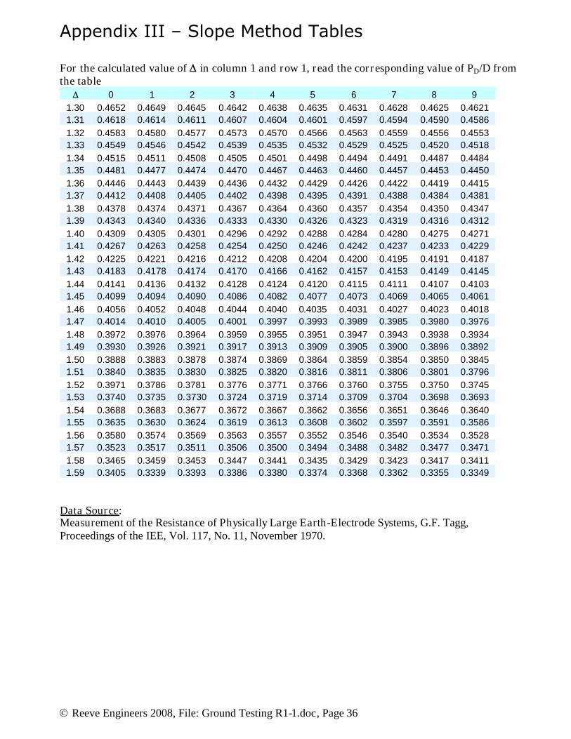
For the calculated value of in column 1 and row 1, read the corresponding value of PD/D fromthe table
0 1 2 3 4 5 6 7 8 91.30 0.4652 0.4649 0.4645 0.4642 0.4638 0.4635 0.4631 0.4628 0.4625 0.46211.31 0.4618 0.4614 0.4611 0.4607 0.4604 0.4601 0.4597 0.4594 0.4590 0.45861.32 0.4583 0.4580 0.4577 0.4573 0.4570 0.4566 0.4563 0.4559 0.4556 0.45531.33 0.4549 0.4546 0.4542 0.4539 0.4535 0.4532 0.4529 0.4525 0.4520 0.45181.34 0.4515 0.4511 0.4508 0.4505 0.4501 0.4498 0.4494 0.4491 0.4487 0.44841.35 0.4481 0.4477 0.4474 0.4470 0.4467 0.4463 0.4460 0.4457 0.4453 0.44501.36 0.4446 0.4443 0.4439 0.4436 0.4432 0.4429 0.4426 0.4422 0.4419 0.44151.37 0.4412 0.4408 0.4405 0.4402 0.4398 0.4395 0.4391 0.4388 0.4384 0.43811.38 0.4378 0.4374 0.4371 0.4367 0.4364 0.4360 0.4357 0.4354 0.4350 0.43471.39 0.4343 0.4340 0.4336 0.4333 0.4330 0.4326 0.4323 0.4319 0.4316 0.43121.40 0.4309 0.4305 0.4301 0.4296 0.4292 0.4288 0.4284 0.4280 0.4275 0.42711.41 0.4267 0.4263 0.4258 0.4254 0.4250 0.4246 0.4242 0.4237 0.4233 0.42291.42 0.4225 0.4221 0.4216 0.4212 0.4208 0.4204 0.4200 0.4195 0.4191 0.41871.43 0.4183 0.4178 0.4174 0.4170 0.4166 0.4162 0.4157 0.4153 0.4149 0.41451.44 0.4141 0.4136 0.4132 0.4128 0.4124 0.4120 0.4115 0.4111 0.4107 0.41031.45 0.4099 0.4094 0.4090 0.4086 0.4082 0.4077 0.4073 0.4069 0.4065 0.40611.46 0.4056 0.4052 0.4048 0.4044 0.4040 0.4035 0.4031 0.4027 0.4023 0.40181.47 0.4014 0.4010 0.4005 0.4001 0.3997 0.3993 0.3989 0.3985 0.3980 0.39761.48 0.3972 0.3976 0.3964 0.3959 0.3955 0.3951 0.3947 0.3943 0.3938 0.39341.49 0.3930 0.3926 0.3921 0.3917 0.3913 0.3909 0.3905 0.3900 0.3896 0.38921.50 0.3888 0.3883 0.3878 0.3874 0.3869 0.3864 0.3859 0.3854 0.3850 0.38451.51 0.3840 0.3835 0.3830 0.3825 0.3820 0.3816 0.3811 0.3806 0.3801 0.37961.52 0.3971 0.3786 0.3781 0.3776 0.3771 0.3766 0.3760 0.3755 0.3750 0.37451.53 0.3740 0.3735 0.3730 0.3724 0.3719 0.3714 0.3709 0.3704 0.3698 0.36931.54 0.3688 0.3683 0.3677 0.3672 0.3667 0.3662 0.3656 0.3651 0.3646 0.36401.55 0.3635 0.3630 0.3624 0.3619 0.3613 0.3608 0.3602 0.3597 0.3591 0.35861.56 0.3580 0.3574 0.3569 0.3563 0.3557 0.3552 0.3546 0.3540 0.3534 0.35281.57 0.3523 0.3517 0.3511 0.3506 0.3500 0.3494 0.3488 0.3482 0.3477 0.34711.58 0.3465 0.3459 0.3453 0.3447 0.3441 0.3435 0.3429 0.3423 0.3417 0.34111.59 0.3405 0.3339 0.3393 0.3386 0.3380 0.3374 0.3368 0.3362 0.3355 0.3349
Data Source:Measurement of the Resistance of Physically Large Earth-Electrode Systems, G.F. Tagg,Proceedings of the IEE, Vol. 117, No. 11, November 1970.
Appendix IV – Slope Method Field Data Form
Reeve Engineers 2008, File: Ground Testing R1-1.doc, Page 37
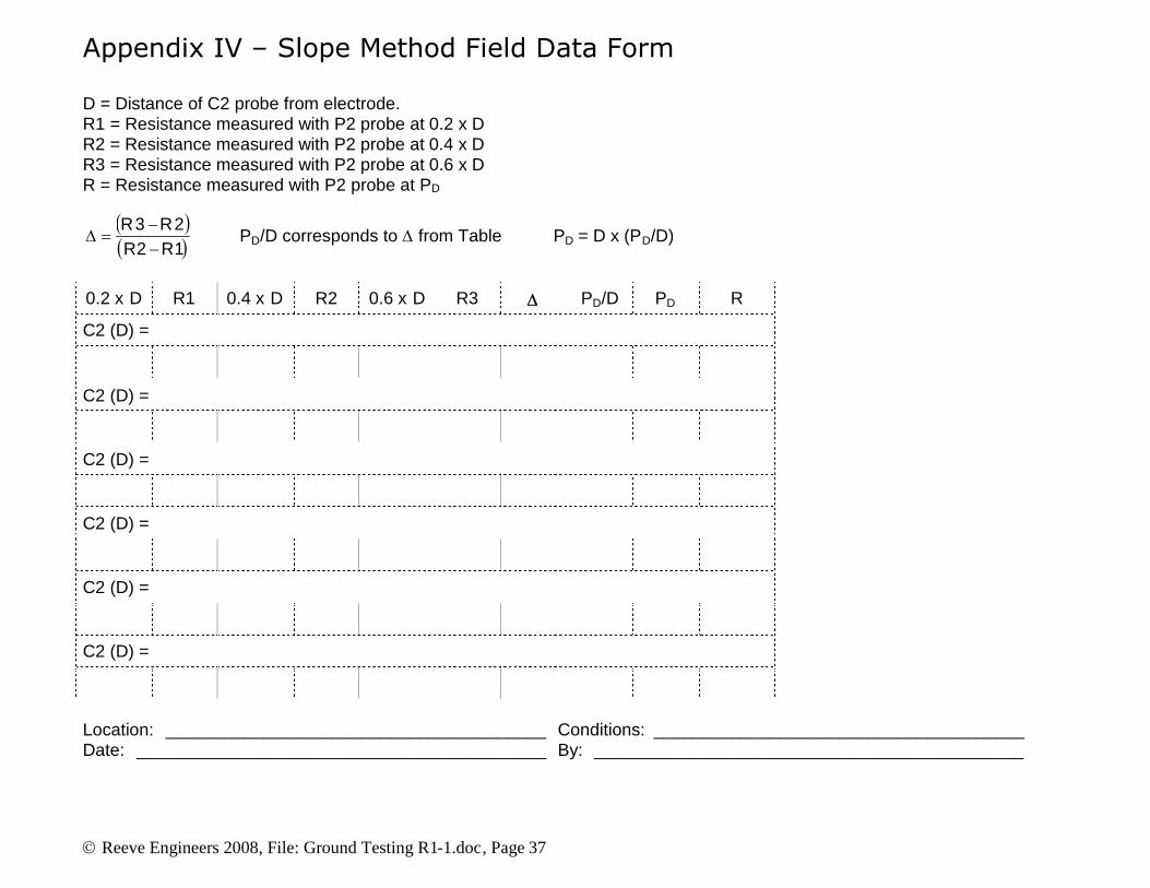
D = Distance of C2 probe from electrode.R1 = Resistance measured with P2 probe at 0.2 x DR2 = Resistance measured with P2 probe at 0.4 x DR3 = Resistance measured with P2 probe at 0.6 x DR = Resistance measured with P2 probe at PD
12
23RRRR
PD/D corresponds to from Table PD = D x (PD/D)
0.2 x D R1 0.4 x D R2 0.6 x D R3 PD/D PD R
C2 (D) =
C2 (D) =
C2 (D) =
C2 (D) =
C2 (D) =
C2 (D) =
Location: _______________________________________ Conditions: ______________________________________Date: __________________________________________ By: ____________________________________________
Appendix V – Soil Resistivity Field Data Form
Reeve Engineers 2008, File: Ground Testing R1-1.doc, Page 38
Spacing (ft)MeasuredR (ohms)
Calculated(ohms-m) Site Info
5 Test Set Model:10 Test Set S/N:15 Ground System Type:20 Temperature:25 Weather:30 Soil Moist or Dry:35 Soil Type (Circle):40 Loam45 Sand & gravel50 Shale55 Clay60 Limestone65 Sandstone70 Granite75 Slate80 Other
Location: _______________________________________________________Conditions: _____________________________________________________Date: __________________________________________________________By: ____________________________________________________________
For spacing (a) measured in ft:
Ra ft 915.1 ohm-m
For spacing (a) measured in m:
Ram 283.6 ohm-m