Vol.:(0123456789)1 3

Acta Geophysica (2019) 67:1823–1834 https://doi.org/10.1007/s11600-019-00338-7

RESEARCH ARTICLE - SPECIAL ISSUE

Geophysical and geotechnical approach to a landslide stability assessment: a case study

Bernadetta Pasierb1 · Michał Grodecki1 · Rafał Gwóźdź1

Received: 30 April 2019 / Accepted: 30 July 2019 / Published online: 17 August 2019 © The Author(s) 2019

AbstractLandslides are complex phenomena, and the main factors that have a significant impact on their behavior are changes in slope inclination geometry and changes in water conditions. The main purpose of this work was to evaluate current conditions of the landslide in Brzozówka, near Cracow (Poland), and analyzing how different saturations of soil influence the stability of the landslide. The combination of geophysical and geotechnical research, such as electrical resistivity tomography (ERT), cone penetration testing, drilling and laboratory tests as well as a comprehensive analysis of their results, provided reliable information on the geological structure and geotechnical parameters of the landslide. The results were used in numerical simulations of the landslide stability, in which a two-phase model (soil and water) was assumed that included the effective soil strength parameters and the transient flow conditions as well as a partial saturation zone. The sliding surface obtained from the numerical modeling was almost flat, which was confirmed by the ERT method. It was proved that the landslide occurred when the saturation of the upper part of the slope exceeded 0.8. Obtained results are useful for engineering practice.

Keywords Numerical analysis of slope stability · Electrical resistivity tomography · Cone penetration testing · Finite element method · Landslide

Introduction

Over the last 20 years, many landslides have occurred in Poland, especially after heavy rainfalls between 1997 and 2002 and in 2010. For appropriate estimation of the crea-tion and stability of the landslide, detailed information about the geological structure and geotechnical parameters of the landslide is necessary. Therefore, noninvasive geophysical methods are very helpful in the study of landslides. They are effective, precise and relatively cheap. They also pro-vide continuous cross section of the geological structure. The increase in the use of geophysical methods has become more widespread due to the efficient data acquisition, digital recording of the measurements and improved procedures

of the processing and interpretation of data. From various geophysical methods (seismic, electrical resistivity tomog-raphy, ground penetrating radar or gravimetric survey) which provide useful information about landslide geometry reconstruction and hydrological characteristics of the place of studies, the electrical resistivity tomography (ERT) is the most efficient and most widely used in the landslides inves-tigations. The ERT method is based on the measurement of electrical resistivity values and their spatial distribution in the subsoil. This method is widely used in evaluating slope deformations and in predicting the surface mass move-ments (Friedel et al. 2006; Jongmans and Garambois 2007; Constantin et al. 2011; Pasierb 2015; Bellanova et al. 2018; Šilhán et al. 2019). In particular, this method is applied for recognitions of lithostratigraphic sequences and the geom-etry of the landslide’s body, identifying the sliding surfaces between the slide material and the underlying bedrock and the location high-water content areas (Panek et al. 2008; Dardé et al. 2013; Holec et al. 2013; Dostál et al. 2014; Tomecka-Suchoń et al. 2017; Crawford and Bryson 2018). It is also used for the building and monitoring of high-reso-lution geological models (both 2D and 3D) and presenting results in a 4D system (Lebourg et al. 2005; Jomard et al.

Paper was presented at the CAGG 2019 Conference “Challenges in Applied Geology and Geophysics” organized at the AGH University of Science and Technology, Krakow, Poland, 10-13 September 2019.

* Bernadetta Pasierb bettka@pk.edu.pl

1 Faculty of Environmental Engineering, Cracow University of Technology, Warszawska 24 St, 31-155 Cracow, Poland

1824 Acta Geophysica (2019) 67:1823–1834

1 3

2010; Chambers et al. 2011; Merritt et al. 2014; Uhlemann et al. 2017; Boyle et al. 2018; Břežný et al. 2018). Informa-tion obtained from ERT method is useful for engineering geologists and geomechanics to define the geological set-ting of the investigated subsoil, reconstruct the geometry of landslide body and volume of the slide material and locate the possible sliding surface and lateral boundaries of the landslide—which are necessary to plan mitigating activities and interventions (installation of a drainage system, stabili-zation of landslide, etc.) (Perrone et al. 2014).

Understanding the factors causing the formation of land-slides, proper numerical modeling of geological structures helps to create the protective systems. According to Corn-forth (2005), landslides are complex phenomena. The main factors which have a significant influence on their behavior include changes in the geometry of the slope and changes in the water conditions (Terzaghi 1950; Wysokiński 2011; Sarah and Daryono 2012; Tang et al. 2018). Due to the com-plexity of the problem, classic geotechnical engineering methods for stability assessments often fail. In this situation, numerical analysis of the stability (usually performed with the use of the c-fi reduction method) can be useful (Griffiths and Lane 1999; Truty et al. 2009; Wysokiński 2011; Zheng et al. 2009; Ozbay and Cabalar 2015; Cho 2016; Xu and Yang 2018), giving possibility to model landslide problems very close to the reality. Results of the stability analysis con-tain stability factor SF, which is the factor between stabiliz-ing and destabilizing forces and mechanism of the possible stability loss—sliding surface. Stability factor SF< 1 means an unstable structure, SF= 1 means the soil structure is on the border between stable and unstable, while SF> 1 means a stable structure. Such simulation is usually performed with the use of the finite element method (FEM). Sometimes the finite difference method (FDM)—examples are given by Stanisz et al. 2012—or the boundary element method (BEM) is used. Typically, plane strain conditions are assumed, a 2D model is constructed and the c-fi reduction algorithm is used for the SF estimation. A traditional approach to the landslide stability (with the use of Fellenius, Bishop, Janbu or similar methods) requires the initial assumption of the stability loss mechanism (the shape of the sliding surface, cylindrical or otherwise), which is a major weakness of this methodology (Ozbay and Cabalar 2015). Introduction of the pore pressure (especially in the transient state, induced by rainfall or flood) is also a serious problem in the traditional approach. The main advantage of the c-fi reduction method is that such an assumption is not necessary, and so the shape and localization of the sliding surface are the result only of the simulation. Therefore, the combination of geological, geophysical and geotechnical methods of investigation and complex analysis of their results allows to obtain reliable information about the geological structure and geotechnical parameters of the landslide.

The main goal of the presented work was to evaluate cur-rent conditions of the landslide in Brzozówka, near Cracow (Poland), and also to show that increased saturation of soil, which was a result of rainfall and/or snowmelt, caused the loss of stability of the slope. Therefore, an analysis of the impact of variable saturation on landslide stability was also conducted.

Geological setting

The Brzozówka village is located in southern Poland, in the northwestern part of the Cracow–Czestochowa Upland, bor-dering the north with Cracow. The morphology of the area is variable. The true altitude ranges from approximately 215 m above sea level in the valley of the Dłubnia River to approxi-mately 400 m in the northern part of the area where the village of Brzozówka is situated. The geological structure of the area includes hills and valleys, which form canyons, as well as terraces, alluvial fans, cones and monadnocks. The oldest rocks are made of plate limestone, which dates back to the Jurassic and Cretaceous periods, and are crossed by faults. In many places on these geological formations, sheets of clay from the Neogene period (Miocene) have also been preserved. The youngest Quaternary formations, with a thickness from a few meters up to tens of meters, create an uneven thick coat of loess and loess clay mixed with sand and gravel. The Quaternary sediments in the river valley are represented mainly by gravel and sand of different grain sizes and the youngest Holocene soils, which developed as silts and gravels. The steep slopes form deep and wide val-leys, which include two main rivers: the Pradnik and the Dłubnia and their tributaries. The water level in the forma-tions of the Jurassic period plays the most important role in developing the hydrogeological relations in the rock struc-ture. Due to intensive farming, these water resources are quite easily degraded. The second water level is formed in Cretaceous rocks, where groundwater is of good quality and the water resources are considerable. Groundwater situated in the Miocene and Quaternary formations is less important due to their limited quantity (Gradziński 1972).

The study area was situated on the southern slope of the Pradnik valley in the Brzozówka village (Fig. 1). The terrain is without buildings and part of it is used for agricultural purposes by private owners. It is covered with meadows, forest and dense bushes in the lower part of the slope. In the central part of the slope, there is a noticeable evidence of landslide movements. Information about the landslide in Brzozówka, which was created as a result of melting snow, comes from the 1950s. The landslide is about 200 m long and 100 m wide, and the colluvium thickness is between 4 m and 6 m. This landslide is classified as a sluff (collapse)

1825Acta Geophysica (2019) 67:1823–1834

1 3

Błażyński et al. 1999). In the following years, periodic land-slide activity has been reported, especially in the spring.

Investigations methods

In order to recognize the subsoil of the analyzed area, geo-physical and geotechnical investigations were carried out. The geophysical surveys using the electrical resistivity tomography method were carried out during dry weather in July 2014. Geotechnical investigations were carried out in stages. The first, geological drilling was carried out in July 2011. In addition, CPTUs were carried out in three series, in the summer and winter seasons: September 2011, December 2012 and September 2014. Numerical simulations of the landslide stability were also carried out.

Electrical resistivity tomography (ERT)

Firstly, geophysical surveys were performed—such order allowed us to determine geotechnical measurement scheme and to conduct a range of laboratory tests. The electrical resistivity tomography (ERT) technique is one of the geo-physical methods, which are based on the study of changes in the electrical field generated by a system of electrodes. The ERT measuring procedure consists of the series of DC electrical resistivity measurements along the examined

profile, where uniformly placed stainless steel electrodes are used. The automated, programmed measurement is taken for all possible combination of electrodes, depending on the selected measured array. The details are given for example (Loke 2014 or Pasierb 2012). The increase in the spacing increases the depth range of research determined in this method for approximately one-fifth of the distance between the extreme electrodes. As a result of measurement, the apparent resistivity of rocks, representing the result of the entire heterogeneous, complex anisotropic layers, is deter-mined in accordance with Ohm’s law. The most commonly used measuring systems are the Wenner–Schlumberger and dipole–dipole arrays due to good depth range and the best horizontal resolution, respectively (Loke 2000; Kneisel and Hauck 2008).

In the presented work, ERT geophysical measurements were taken using ARES designed by GF Instruments. The Schlumberger array, which is sensitive to vertical structures and characterized by the maximum depth of penetration, was used. The distance between each electrode was 5.5 m. The electrical resistivity tomography measurements taken along the slope were taken on the profile Brzozówka I of 258.5 m length, which allowed to recognition of the sub-soil to a depth of about 52 m. In addition, a second meas-urement was taken on the same profile the “roll along” method, extending it, by post-measuring subsequent sec-tions, from the beginning to the end of the profile. In this

Fig. 1 Study area and location of geophysical profiles and geotechnical boreholes

1826 Acta Geophysica (2019) 67:1823–1834

1 3

way, a measurement on the Brzozówka II profile could have been taken over a distance of 346.5 m. The range of investi-gation depth in this measurement was reduced to 40 m, due to previously recognized subsoil down to limestone forma-tion. Therefore, the measurement time was shortened and the battery consumption was reduced. The assumed acceptable standard deviation was 5%, and the minimum stacks were set to 4. This meant that if the four data cycles collected at each point fell within 5% of each other, then data col-lection is completed at that data point after the number of stacks set. However, if the acceptable standard deviation was exceeded for a data point, another cycle is completed and the four readings closest together are averaged. The interpreta-tion of ERT survey was done in the RES2DINV software (Geotomo Software—Loke 2014), using a nonlinear opti-mization technique with a 2D inversion process. A detailed description of the inversion algorithms can be found in the works, e.g., Marquardt (1970), Farquharson and Oldenburg (1998), Loke and Dahlin (2002), Aster et al. (2005), Loke (2017). The aim of the inversion is to minimize the error, which determines the degree of discrepancy between cal-culated apparent resistivity values for the assumed and the input model. Three methods of inversion are possible in RES2DINV program: the standard least-squares inversion, smoothness constrain and robust inversion. (A more detailed description is contained in Pasierb 2015.) The standard and similarly smoothness constrain methods, classified as a L2 norm, are based on least-squared optimization method that minimizes the sum of squares (RMS error) of the spatial changes in the model resistivity values. The smoothness constrain inversion method is a slightly modified form of standard inversion including flatness filter and is the most suitable where subsurface resistivity changes continuously in a smooth manner as in the case of pollution plume. The sum of squares (RMS error) is calculated by these methods. The robust inversion—the blocky or L1 norm optimization—generates models consisting of a fixed resistivity value with clearly sharp and straight boundaries. This method is based on minimizing the sum of the absolute difference between measured and calculated apparent resistivities, by the calcu-lation of an absolute error (Abs). The applied L1 minimiza-tion to data results in sharpening the boundaries between geological layers and causes reduction in the impact of the major differences between the values of the model—this gives lower values of error (Loke et al. 2003). In subse-quent iterations, the assumed theoretical model is succes-sively modified until acceptable accuracy is achieved. The calculations also take into account the terrain layout includ-ing the topography in the data processing (Loke 2000). The use of advanced computational techniques, the introduction of external conditions described as a priori information (e.g., geological information) and the imposition of boundary con-ditions controlling the change of the model (as there are

many possible resistivity models of the medium with the same solution) cause a reduction in ambiguous solutions and help to get the two-dimensional distribution of the electrical resistivity medium as close as possible to the distribution of actual resistivity in the subsoil study.

Geotechnical measurements

In order to obtain more complete interpretation and to analyze the correlation between the lithology of the land-slides and determined distribution of electrical resistivity on the profile, a drilling test was carried out using hand methods. The boreholes with a diameter of 0.1 m and a depth of 5 to 9 m below ground level were made at seven sites within 71 m, 100 m, 137 m, 153 m, 200 m, 220 m and 250 m from the beginning of the profile. The loca-tions of geophysical profiles and geotechnical boreholes are shown in Fig. 1.

The geological drilling identified a detailed geological profile. During drilling, the macroscopic analysis of soils was performed, the level of groundwater was determined and samples were taken for the laboratory tests. In the area of the landslide, geotechnical surveys were also carried out to identify ground conditions and to determine the geotechnical parameters of soils using a cone penetration testing (CPTU). The CPTU probe of the Swedish company ENVI with a diameter of 36 mm was used in the research. The CPTU is currently the most popular and the most comprehensive in situ method for identifying geotechnical parameters of the substrate. In addition, the CPTU allows determining the geological structure of the substrate, enabling accurate sepa-ration of weak layers, such as slip planes in landslides. It also allows the estimation of geotechnical parameters based on different conversion formulas and correlations with the natural state of stresses, grain size and humidity of the soil (Lunne et al. 1997).

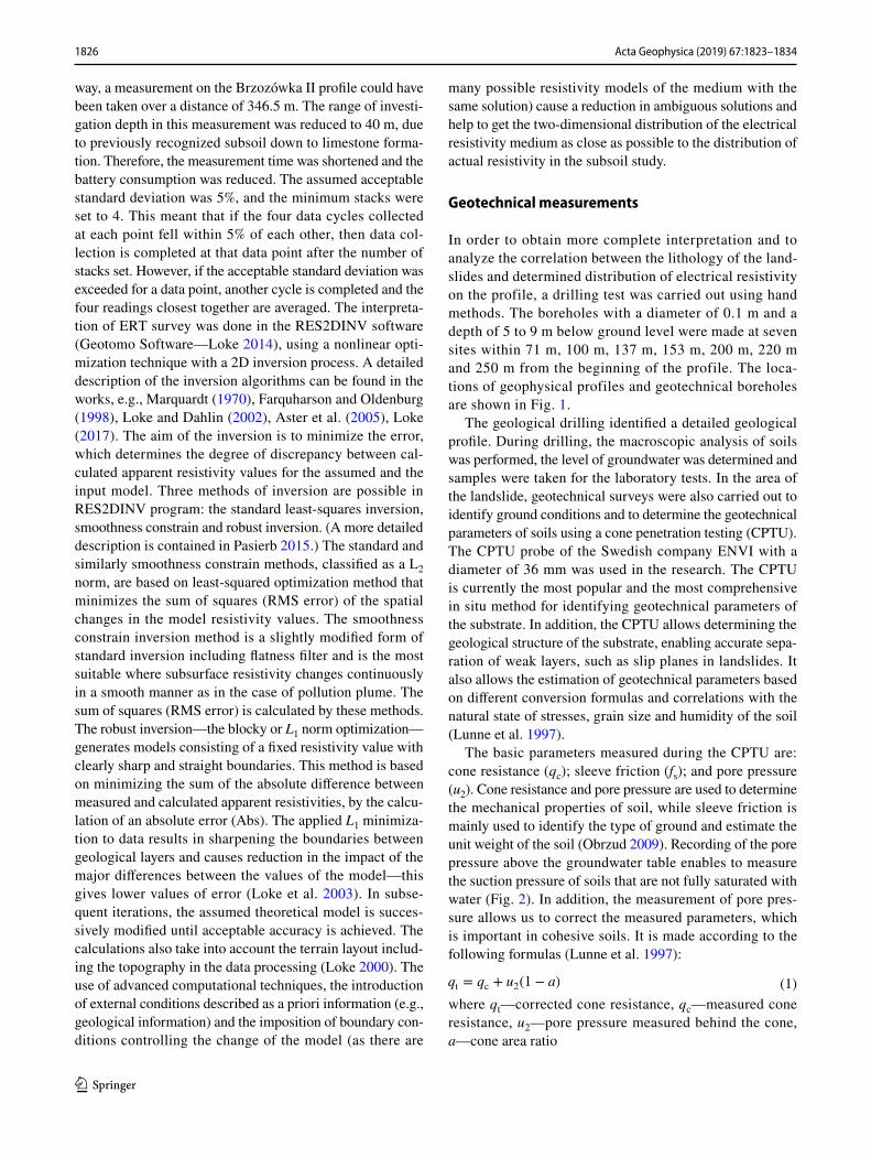
The basic parameters measured during the CPTU are: cone resistance (qc); sleeve friction (fs); and pore pressure (u2). Cone resistance and pore pressure are used to determine the mechanical properties of soil, while sleeve friction is mainly used to identify the type of ground and estimate the unit weight of the soil (Obrzud 2009). Recording of the pore pressure above the groundwater table enables to measure the suction pressure of soils that are not fully saturated with water (Fig. 2). In addition, the measurement of pore pres-sure allows us to correct the measured parameters, which is important in cohesive soils. It is made according to the following formulas (Lunne et al. 1997):

where qt—corrected cone resistance, qc—measured cone resistance, u2—pore pressure measured behind the cone, a—cone area ratio

(1)qt = qc + u2(1 − a)

1827Acta Geophysica (2019) 67:1823–1834

1 3

where Rf—friction ratio, fs—sleeve friction, qt—corrected cone resistance.

Laboratory tests were carried out on soil samples of silt layer above the sliding surface and the underlying clay lay-ers. The study determined the type of soil, physical param-eters (water content, bulk density, plastic and liquid limits) and mechanical parameters (the angle of effective inter-nal friction ϕ‘ and effective cohesion c’). The research of mechanical parameters was carried out using the triaxial compression test. (The method involves research with the initial isotropic consolidation and measurement of pore pressure while compressing.) The study was carried out at a consolidation pressure (σ3, of 75 kPa, 150 kPa, 300 kPa and 600 kPa). The interpretation of test results was conducted using the Coulomb–Mohr theory specifying values for effec-tive stress (Head 1995).

(2)Rf =fs

qt× 100%

Numerical simulations of the landslide

The numerical model constructed using the ZSoil FEM sys-tem (described in detail by Commend et al. 2016) was used to simulate landslide behavior. The FEM model was two-dimensional (2D), with plane strain conditions. In addition, the Coulomb–Mohr constitutive model was assumed with non-associative flow rule: dilatancy angle ψ = 0 for clay and ψ = ϕ/2 for silt. The c-fi reduction algorithm was used for the SF esti-mation. Typical geotechnical boundary conditions for solid phase were assumed—there were no vertical and horizontal displacements on bottom edge, no horizontal displacements on lateral edges and no normal stress on the top edge. Numeri-cal model consisted of 2375 quadrilateral elements and 2867 nodes. Enhanced assumed strain (EAS) elements were used (Simo and Rifai 1990). Unsteady filtration state (infiltration due to rainfall) was considered, and analysis was performed in the effective stresses. The presented approach is novel, because usually in the engineering practice stability is analyzed in the total stresses, using total soil strength parameters (cohesion and friction angle), which depend on the saturation of the soil. In this article, analysis is performed in effective stresses with the use of effective cohesion and friction angle (which do not depend on the saturation). This approach does not require esti-mation of the soil parameters for different saturations of soils, which decreases the amount of the laboratory works. An addi-tional advantage of the proposed approach, in opposite to the traditional approach with the use of Fellenius, Bishop, Janbu or similar methods, is that the initial assumption of the stability loss mechanism (shape of the sliding surface—cylindrical or other) is not required—shape and location of the failure surface are the result of the simulation. In the case of having the results of geophysical research, the assumed shape of the sliding sur-face is a confirmation of the correctness of the simulation.

The overview of the calculations algorithm used in the c-fi reduction algorithm is presented below: The state of the stress at a certain phase of simulation is determined with the use of elasto-plastic soil constitutive model (usually Cou-lomb–Mohr model). If equilibrium conditions are fulfilled, the initial value SF= 1 is assumed as the current value of the SF, friction angle and cohesion are modified according to formulas (3):

The elasto-plastic analysis is performed again for reduced parameters of the soil. If equilibrium conditions are fulfilled, the process of the reduction is continued according to the for-mulas above. If equilibrium conditions are not fulfilled, diver-gence of the iteration process occurs and the stability analysis

(3)

SF(i) = SF(i−1) + ΔSF

(tg)(i) = (tg)(o)∕SF(i)

c(i)= c

(o)∕SF(i)

saSi - Si

Type of soils

siCl - Cl

weak layer

ClSa

saGr

clSi - Si

3.0

4.0

2.0

1.0

0.0

5.0

6.0

8.0

9.0

qt [MPa] fs [kPa] u2 [kPa] Rf [%]0 1 2 3 4 5 0 100 200 0 400 800 0 2 4 6

7.0

Fig. 2 Static sounding profile CPTU and characteristic soil parame-ters. Type of soils: saSi—sandy silt, Si—silt, clSi—clayey silt, siCl—silty clay, Cl—clay, Sa—sand, saGr—sandy gravel

1828 Acta Geophysica (2019) 67:1823–1834

1 3

ends up. The SF value for last converged step is assumed as an estimation of the SF of the structure. Increment ΔSF could be as low as needed; however, usually values lower than 0.01 are not required. The displacements obtained in the moment of the stability loss do not have physical meaning—they only illustrate the stability loss mechanism. The c-fi reduction algo-rithm works for both 2D and 3D problems. This approach is fully consistent with Eurocode 7. More detailed description of this procedure and other issues of the computer modeling of landslides are given by Griffiths and Lane (1999), Truty et al. (2009), Wysokiński (2011) and Zheng et al. (2009).

In the presented work, transient flow conditions were used and the effect of the rainfall is modeled with use of the flow model with description of the partially saturated zone pro-posed by Van Genuchten (1980). Modified form of Darcy law, valid for both fully and partially saturated zones, was used, with conductivity dependent on pressures.

where k—Darcy coefficient for saturated soil, S—saturation ratio (0 ≤ S ≤ 1), Z ≡ y—gravity potential, γ—water specific weight, kr—function relating conductivity to saturation ratio:

where Sr—residual saturation. Relationship between satura-tion and pressure is presented (6):

(4)q = −k ⋅ kr(S(p)) ⋅ grad(−p∕ + Z)

(5)kr(S) =

1 for S = 1(S−Sr)

3

(1−Sr)3

for S < 1

(6)S = S(p) =

1 for p ≤ 0

Sr +1−Sr

[

1+(𝛼p∕𝛾)2]0.5 for p > 0

where α is the parameter controlling width of transition layer above the free surface. In the fully saturated zone, linear Darcy’s law holds. Continuity equation (Richards’s equa-tion) completes the model:

where β—fluid bulk modulus, n (0 < n < 1)—porosity (being additional characteristic of the soil), v—volumetric strain ratio. The presence of strain term causes coupling of flow with soil deformation.

Results and discussion

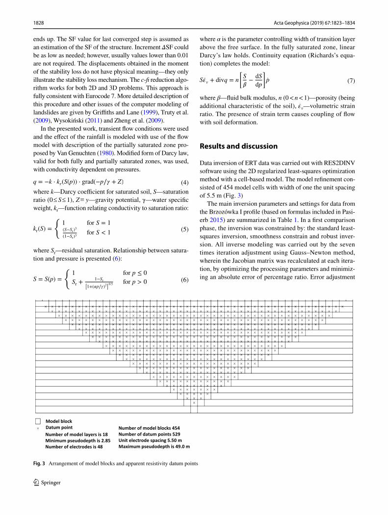
Data inversion of ERT data was carried out with RES2DINV software using the 2D regularized least-squares optimization method with a cell-based model. The model refinement con-sisted of 454 model cells with width of one the unit spacing of 5.5 m (Fig. 3)

The main inversion parameters and settings for data from the Brzozówka I profile (based on formulas included in Pasi-erb 2015) are summarized in Table 1. In a first comparison phase, the inversion was constrained by: the standard least-squares inversion, smoothness constrain and robust inver-sion. All inverse modeling was carried out by the seven times iteration adjustment using Gauss–Newton method, wherein the Jacobian matrix was recalculated at each itera-tion, by optimizing the processing parameters and minimiz-ing an absolute error of percentage ratio. Error adjustment

(7)Sv + divq = n

[

S

𝛽−

dS

dp

]

p

Model blockDatum pointNumber of model layers is 18Minimum pseudodepth is 2.85Number of electrodes is 48

Number of model blocks 454Number of datum points 529Unit electrode spacing 5.50 mMaximum pseudodepth is 49.0 m

Fig. 3 Arrangement of model blocks and apparent resistivity datum points

1829Acta Geophysica (2019) 67:1823–1834

1 3

for all inversions was the same (abs. error = 1.1), while a slight difference could be seen in the image of the resistivity distribution.

Based on the calculations and the analysis of the obtained cross-sectional distribution of electrical resistivity, the L1 norm inversion method (robust inversion) has given optimal results for the analyzed subsoil compared to the two other methods of inversion. Thus, in the implemented 2D inversion process, the robust model inversion constraint was used in a further processing. Also, in processing of the data obtained

from measurements for Brzozówka II profile–where the “roll along” method was applied–robust inversion was used and absolute error was 0.67.

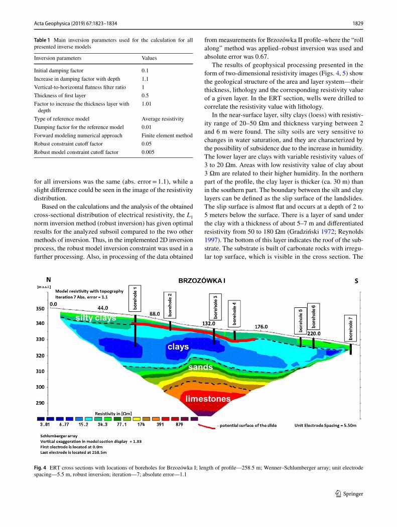
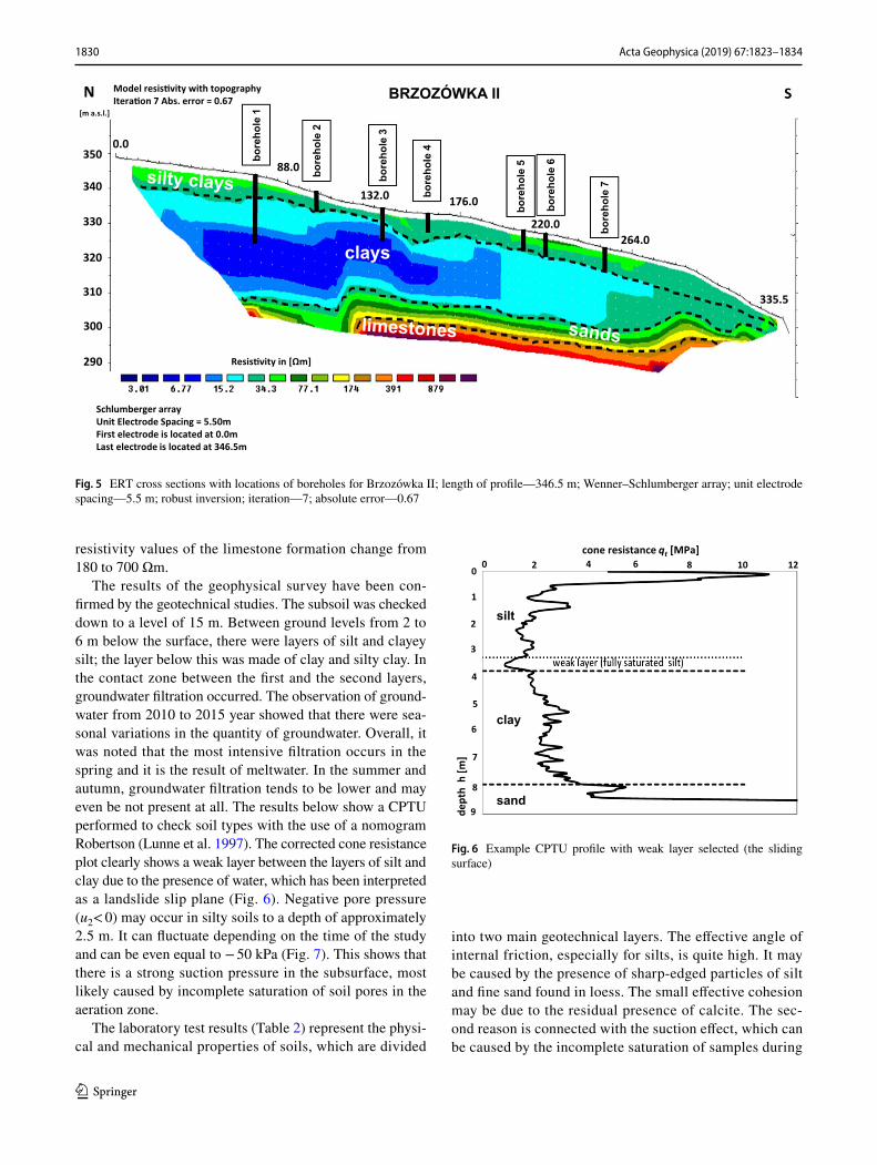
The results of geophysical processing presented in the form of two-dimensional resistivity images (Figs. 4, 5) show the geological structure of the area and layer system—their thickness, lithology and the corresponding resistivity value of a given layer. In the ERT section, wells were drilled to correlate the resistivity value with lithology.

In the near-surface layer, silty clays (loess) with resistiv-ity range of 20–50 Ωm and thickness varying between 2 and 6 m were found. The silty soils are very sensitive to changes in water saturation, and they are characterized by the possibility of subsidence due to the increase in humidity. The lower layer are clays with variable resistivity values of 3 to 20 Ωm. Areas with low resistivity value of clay about 3 Ωm are related to their higher humidity. In the northern part of the profile, the clay layer is thicker (ca. 30 m) than in the southern part. The boundary between the silt and clay layers can be defined as the slip surface of the landslides. The slip surface is almost flat and occurs at a depth of 2 to 5 meters below the surface. There is a layer of sand under the clay with a thickness of about 5–7 m and differentiated resistivity from 50 to 180 Ωm (Gradziński 1972; Reynolds 1997). The bottom of this layer indicates the roof of the sub-strate. The substrate is built of carbonate rocks with irregu-lar top surface, which is visible in the cross section. The

Table 1 Main inversion parameters used for the calculation for all presented inverse models

Inversion parameters Values

Initial damping factor 0.1Increase in damping factor with depth 1.1Vertical-to-horizontal flatness filter ratio 1Thickness of first layer 0.5Factor to increase the thickness layer with

depth1.01

Type of reference model Average resistivityDamping factor for the reference model 0.01Forward modeling numerical approach Finite element methodRobust constraint cutoff factor 0.05Robust model constraint cutoff factor 0.005

Fig. 4 ERT cross sections with locations of boreholes for Brzozówka I; length of profile—258.5 m; Wenner–Schlumberger array; unit electrode spacing—5.5 m, robust inversion; iteration—7; absolute error—1.1

1830 Acta Geophysica (2019) 67:1823–1834

1 3

resistivity values of the limestone formation change from 180 to 700 Ωm.

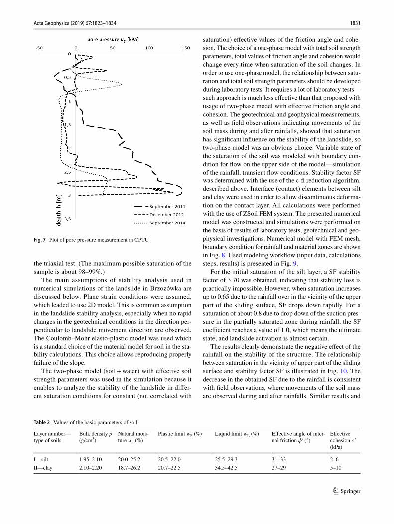
The results of the geophysical survey have been con-firmed by the geotechnical studies. The subsoil was checked down to a level of 15 m. Between ground levels from 2 to 6 m below the surface, there were layers of silt and clayey silt; the layer below this was made of clay and silty clay. In the contact zone between the first and the second layers, groundwater filtration occurred. The observation of ground-water from 2010 to 2015 year showed that there were sea-sonal variations in the quantity of groundwater. Overall, it was noted that the most intensive filtration occurs in the spring and it is the result of meltwater. In the summer and autumn, groundwater filtration tends to be lower and may even be not present at all. The results below show a CPTU performed to check soil types with the use of a nomogram Robertson (Lunne et al. 1997). The corrected cone resistance plot clearly shows a weak layer between the layers of silt and clay due to the presence of water, which has been interpreted as a landslide slip plane (Fig. 6). Negative pore pressure (u2< 0) may occur in silty soils to a depth of approximately 2.5 m. It can fluctuate depending on the time of the study and can be even equal to − 50 kPa (Fig. 7). This shows that there is a strong suction pressure in the subsurface, most likely caused by incomplete saturation of soil pores in the aeration zone.

The laboratory test results (Table 2) represent the physi-cal and mechanical properties of soils, which are divided

into two main geotechnical layers. The effective angle of internal friction, especially for silts, is quite high. It may be caused by the presence of sharp-edged particles of silt and fine sand found in loess. The small effective cohesion may be due to the residual presence of calcite. The sec-ond reason is connected with the suction effect, which can be caused by the incomplete saturation of samples during

290

300

310

320

330

340

350

BRZOZÓWKA II

Resisvity in [Ωm]

Schlumberger arrayUnit Electrode Spacing = 5.50mFirst electrode is located at 0.0mLast electrode is located at 346.5m

Model resisvity with topographyIteraon 7 Abs. error = 0.67

88.0

176.0

264.0

0.0

clays

335.5

bore

hole

1

bore

hole

2

bore

hole

3

bore

hole

4

bore

hole

5

bore

hole

6

bore

hole

7

132.0

220.0

N[m a.s.l.]

Fig. 5 ERT cross sections with locations of boreholes for Brzozówka II; length of profile—346.5 m; Wenner–Schlumberger array; unit electrode spacing—5.5 m; robust inversion; iteration—7; absolute error—0.67

dept

h h

[m]

silt

clay

sand

0 2 4 6 8 10 120

1

2

3

4

5

6

7

8

9

cone resistance qt [MPa]

Fig. 6 Example CPTU profile with weak layer selected (the sliding surface)

1831Acta Geophysica (2019) 67:1823–1834

1 3

the triaxial test. (The maximum possible saturation of the sample is about 98–99%.)

The main assumptions of stability analysis used in numerical simulations of the landslide in Brzozówka are discussed below. Plane strain conditions were assumed, which leaded to use 2D model. This is common assumption in the landslide stability analysis, especially when no rapid changes in the geotechnical conditions in the direction per-pendicular to landslide movement direction are observed. The Coulomb–Mohr elasto-plastic model was used which is a standard choice of the material model for soil in the sta-bility calculations. This choice allows reproducing properly failure of the slope.

The two-phase model (soil + water) with effective soil strength parameters was used in the simulation because it enables to analyze the stability of the landslide in differ-ent saturation conditions for constant (not correlated with

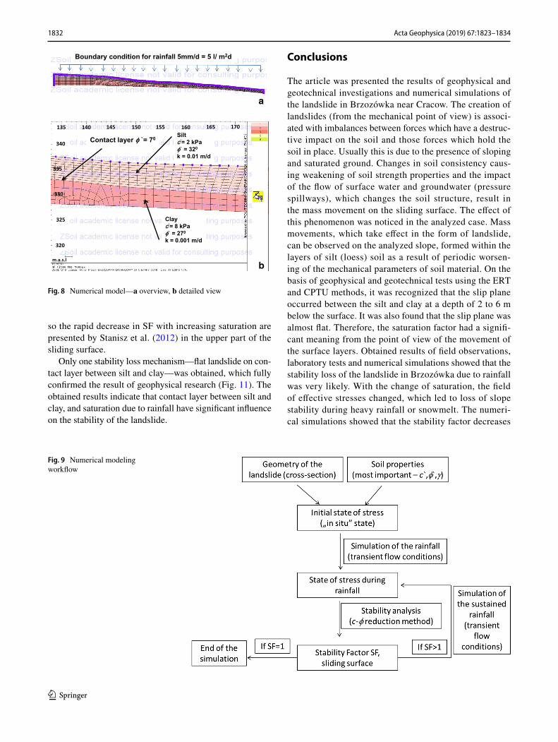
saturation) effective values of the friction angle and cohe-sion. The choice of a one-phase model with total soil strength parameters, total values of friction angle and cohesion would change every time when saturation of the soil changes. In order to use one-phase model, the relationship between satu-ration and total soil strength parameters should be developed during laboratory tests. It requires a lot of laboratory tests—such approach is much less effective than that proposed with usage of two-phase model with effective friction angle and cohesion. The geotechnical and geophysical measurements, as well as field observations indicating movements of the soil mass during and after rainfalls, showed that saturation has significant influence on the stability of the landslide, so two-phase model was an obvious choice. Variable state of the saturation of the soil was modeled with boundary con-dition for flow on the upper side of the model—simulation of the rainfall, transient flow conditions. Stability factor SF was determined with the use of the c-fi reduction algorithm, described above. Interface (contact) elements between silt and clay were used in order to allow discontinuous deforma-tion on the contact layer. All calculations were performed with the use of ZSoil FEM system. The presented numerical model was constructed and simulations were performed on the basis of results of laboratory tests, geotechnical and geo-physical investigations. Numerical model with FEM mesh, boundary condition for rainfall and material zones are shown in Fig. 8. Used modeling workflow (input data, calculations steps, results) is presented in Fig. 9.

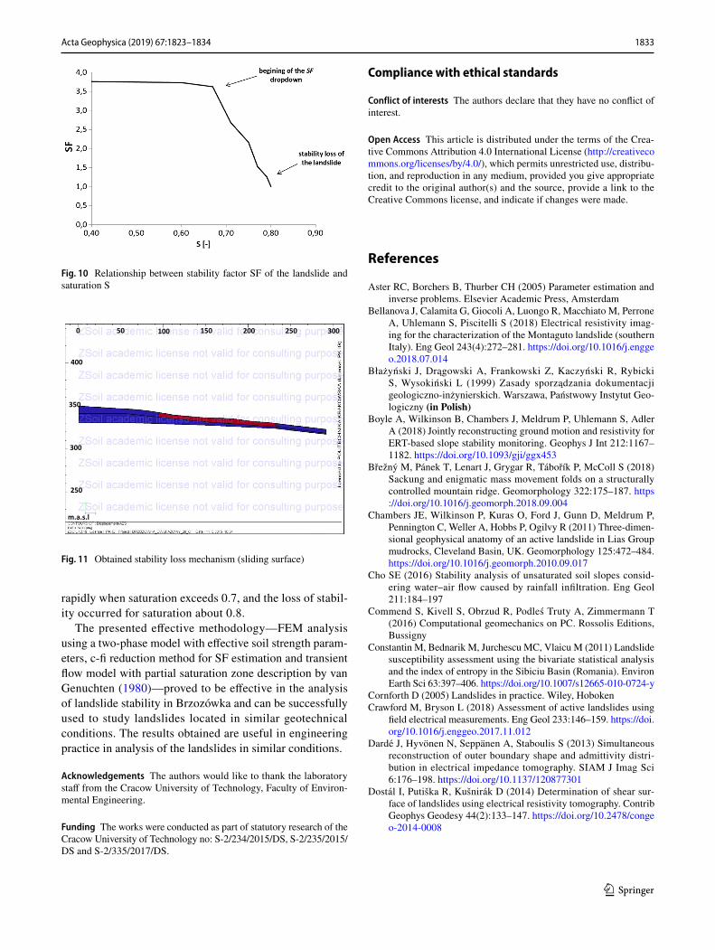
For the initial saturation of the silt layer, a SF stability factor of 3.70 was obtained, indicating that stability loss is practically impossible. However, when saturation increases up to 0.65 due to the rainfall over in the vicinity of the upper part of the sliding surface, SF drops down rapidly. For a saturation of about 0.8 due to drop down of the suction pres-sure in the partially saturated zone during rainfall, the SF coefficient reaches a value of 1.0, which means the ultimate state, and landslide activation is almost certain.

The results clearly demonstrate the negative effect of the rainfall on the stability of the structure. The relationship between saturation in the vicinity of upper part of the sliding surface and stability factor SF is illustrated in Fig. 10. The decrease in the obtained SF due to the rainfall is consistent with field observations, where movements of the soil mass are observed during and after rainfalls. Similar results and

Fig. 7 Plot of pore pressure measurement in CPTU

Table 2 Values of the basic parameters of soil

Layer number—type of soils

Bulk density ρ (g/cm3)

Natural mois-ture wn (%)

Plastic limit wP (%) Liquid limit wL (%) Effective angle of inter-nal friction ϕʹ (°)

Effective cohesion cʹ (kPa)

I—silt 1.95–2.10 20.0–25.2 20.5–22.0 25.5–29.3 31–33 2–6II—clay 2.10–2.20 18.7–26.2 20.7–22.5 34.5–42.5 27–29 5–10

1832 Acta Geophysica (2019) 67:1823–1834

1 3

so the rapid decrease in SF with increasing saturation are presented by Stanisz et al. (2012) in the upper part of the sliding surface.

Only one stability loss mechanism—flat landslide on con-tact layer between silt and clay—was obtained, which fully confirmed the result of geophysical research (Fig. 11). The obtained results indicate that contact layer between silt and clay, and saturation due to rainfall have significant influence on the stability of the landslide.

Conclusions

The article was presented the results of geophysical and geotechnical investigations and numerical simulations of the landslide in Brzozówka near Cracow. The creation of landslides (from the mechanical point of view) is associ-ated with imbalances between forces which have a destruc-tive impact on the soil and those forces which hold the soil in place. Usually this is due to the presence of sloping and saturated ground. Changes in soil consistency caus-ing weakening of soil strength properties and the impact of the flow of surface water and groundwater (pressure spillways), which changes the soil structure, result in the mass movement on the sliding surface. The effect of this phenomenon was noticed in the analyzed case. Mass movements, which take effect in the form of landslide, can be observed on the analyzed slope, formed within the layers of silt (loess) soil as a result of periodic worsen-ing of the mechanical parameters of soil material. On the basis of geophysical and geotechnical tests using the ERT and CPTU methods, it was recognized that the slip plane occurred between the silt and clay at a depth of 2 to 6 m below the surface. It was also found that the slip plane was almost flat. Therefore, the saturation factor had a signifi-cant meaning from the point of view of the movement of the surface layers. Obtained results of field observations, laboratory tests and numerical simulations showed that the stability loss of the landslide in Brzozówka due to rainfall was very likely. With the change of saturation, the field of effective stresses changed, which led to loss of slope stability during heavy rainfall or snowmelt. The numeri-cal simulations showed that the stability factor decreases

325

330

335

340

320

135 140 145 150 155 160 165 170

Contact layer φ `= 70

Clay c ’= 8 kPaφ` = 270

k = 0.001 m/d

Siltc ’= 2 kPaφ` = 320

k = 0.01 m/d

Boundary condition for rainfall 5mm/d = 5 l/ m2d

m.a.s.l

a

b

Fig. 8 Numerical model—a overview, b detailed view

Fig. 9 Numerical modeling workflow

1833Acta Geophysica (2019) 67:1823–1834

1 3

rapidly when saturation exceeds 0.7, and the loss of stabil-ity occurred for saturation about 0.8.

The presented effective methodology—FEM analysis using a two-phase model with effective soil strength param-eters, c-fi reduction method for SF estimation and transient flow model with partial saturation zone description by van Genuchten (1980)—proved to be effective in the analysis of landslide stability in Brzozówka and can be successfully used to study landslides located in similar geotechnical conditions. The results obtained are useful in engineering practice in analysis of the landslides in similar conditions.

Acknowledgements The authors would like to thank the laboratory staff from the Cracow University of Technology, Faculty of Environ-mental Engineering.

Funding The works were conducted as part of statutory research of the Cracow University of Technology no: S-2/234/2015/DS, S-2/235/2015/DS and S-2/335/2017/DS.

Compliance with ethical standards

Conflict of interests The authors declare that they have no conflict of interest.

Open Access This article is distributed under the terms of the Crea-tive Commons Attribution 4.0 International License (http://creat iveco mmons .org/licen ses/by/4.0/), which permits unrestricted use, distribu-tion, and reproduction in any medium, provided you give appropriate credit to the original author(s) and the source, provide a link to the Creative Commons license, and indicate if changes were made.

References

Aster RC, Borchers B, Thurber CH (2005) Parameter estimation and inverse problems. Elsevier Academic Press, Amsterdam

Bellanova J, Calamita G, Giocoli A, Luongo R, Macchiato M, Perrone A, Uhlemann S, Piscitelli S (2018) Electrical resistivity imag-ing for the characterization of the Montaguto landslide (southern Italy). Eng Geol 243(4):272–281. https ://doi.org/10.1016/j.engge o.2018.07.014

Błażyński J, Drągowski A, Frankowski Z, Kaczyński R, Rybicki S, Wysokiński L (1999) Zasady sporządzania dokumentacji geologiczno-inżynierskich. Warszawa, Państwowy Instytut Geo-logiczny (in Polish)

Boyle A, Wilkinson B, Chambers J, Meldrum P, Uhlemann S, Adler A (2018) Jointly reconstructing ground motion and resistivity for ERT-based slope stability monitoring. Geophys J Int 212:1167–1182. https ://doi.org/10.1093/gji/ggx45 3

Břežný M, Pánek T, Lenart J, Grygar R, Tábořík P, McColl S (2018) Sackung and enigmatic mass movement folds on a structurally controlled mountain ridge. Geomorphology 322:175–187. https ://doi.org/10.1016/j.geomo rph.2018.09.004

Chambers JE, Wilkinson P, Kuras O, Ford J, Gunn D, Meldrum P, Pennington C, Weller A, Hobbs P, Ogilvy R (2011) Three-dimen-sional geophysical anatomy of an active landslide in Lias Group mudrocks, Cleveland Basin, UK. Geomorphology 125:472–484. https ://doi.org/10.1016/j.geomo rph.2010.09.017

Cho SE (2016) Stability analysis of unsaturated soil slopes consid-ering water–air flow caused by rainfall infiltration. Eng Geol 211:184–197

Commend S, Kivell S, Obrzud R, Podleś Truty A, Zimmermann T (2016) Computational geomechanics on PC. Rossolis Editions, Bussigny

Constantin M, Bednarik M, Jurchescu MC, Vlaicu M (2011) Landslide susceptibility assessment using the bivariate statistical analysis and the index of entropy in the Sibiciu Basin (Romania). Environ Earth Sci 63:397–406. https ://doi.org/10.1007/s1266 5-010-0724-y

Cornforth D (2005) Landslides in practice. Wiley, HobokenCrawford M, Bryson L (2018) Assessment of active landslides using

field electrical measurements. Eng Geol 233:146–159. https ://doi.org/10.1016/j.engge o.2017.11.012

Dardé J, Hyvönen N, Seppänen A, Staboulis S (2013) Simultaneous reconstruction of outer boundary shape and admittivity distri-bution in electrical impedance tomography. SIAM J Imag Sci 6:176–198. https ://doi.org/10.1137/12087 7301

Dostál I, Putiška R, Kušnirák D (2014) Determination of shear sur-face of landslides using electrical resistivity tomography. Contrib Geophys Geodesy 44(2):133–147. https ://doi.org/10.2478/conge o-2014-0008

Fig. 10 Relationship between stability factor SF of the landslide and saturation S

350

300

250

400

0 50 100 150 200 250

m.a.s.l

300

Fig. 11 Obtained stability loss mechanism (sliding surface)

1834 Acta Geophysica (2019) 67:1823–1834

1 3

Farquharson CG, Oldenburg DW (1998) Non-linear inversion using general measures of data misfit and model structure. Geophys J Int 134:213–227. https ://doi.org/10.1046/j.1365-246x.1998.00555

Friedel S, Thielen A, Springman SM (2006) Investigation of a slope endangered by rainfall-induced landslides using 3D resistivity tomography and geotechnical testing. J Appl Geophys 60:100–114. https ://doi.org/10.1016/j.jappg eo.2006.01.001

Gradziński R (1972) Geological guide the vicinity of Cracow, 1st edn. Geological Press, Warsaw (in Polish)

Griffiths DV, Lane PA (1999) Slope stability analysis by finite ele-ments. Geotechnique 49(3):387–403. https ://doi.org/10.1680/geot.1999.49.3.387

Head KH (1995) Manual of soil laboratory testing, II edn. Pentech Press, London

Holec J, Bednarik M, Sabo M, Minar J, Yilmaz I, Marschalko M (2013) A small-scale landslide susceptibility assessment for the territory of Western Carpathians. Nat Hazard 69:1081–1107. https ://doi.org/10.1007/s1106 9-013-0751-6

Jomard H, Lebourg T, Guglielmi Y, Tric E (2010) Electrical imaging of sliding geometry and fluids associated with a deep seated land-slide (La Clapiere, France). Earth Surf Proc Land 35:588–599. https ://doi.org/10.1002/esp.1941

Jongmans D, Garambois S (2007) Geophysical investigation of land-slides: a review. Bull Soc France 178(2):101–112. https ://doi.org/10.2113/gssgf bull.178.2.101

Kneisel C, Hauck C (2008) Electrical method. In: Hauck C, Kneisel C (eds) Applied geophysics in periglacial environments. Cambridge University Press, Cambridge, pp 3–27

Lebourg T, Binet S, Tric E, Jomarad H, Bedoui SE (2005) Geophysical survey to estimate the 3D sliding surface and the 4D evolution of the water pressure on part of a deep seated landslide. Terra Nova 17(5):399–406. https ://doi.org/10.1111/j.1365-3121.2005.00623

Loke M (2000) Topographic modelling in electrical imaging inversion. In: 62nd EAGE conference and technical exhibition: Glasgow, Scotland, 29 May–2 June 2000, Extended Abstracts, D-2

Loke M (2014) Tutorial: 2-D and 3-D electrical imagining surveys. Geotomo Software, Malaysia

Loke MH (2017) Rapid 3-D resistivity & IP inversion using the least-squares method. Geotomo software, Penang Malaysia

Loke M, Dahlin T (2002) A comparison of the Gauss- Newton and quasi-Newton methods in resistivity imaging inversion. J Appl Geophys 49:149–162. https ://doi.org/10.1016/S0926 -9851(01)00106 -9

Loke M, Ackworth I, Dahlin T (2003) A comparison of smooth and blocky inversion methods in 2D electrical imaging surveys. Explor Geophys 34:182–187. https ://doi.org/10.1071/EG031 82

Lunne T, Robertson P, Powell J (1997) Cone Penetration Testing in geotechnical practice. Blackie Academic and Professional, London

Marquardt D (1970) Generalized inverse, ridge regression, biased linear estimation and nonlinear regression. Technometrics 12:591–613

Merritt A, Chambers J, Murphy W, Wilkinson P, West L, Gunn D, Mel-drum P, Kirkham M, Dixon N (2014) 3D ground model develop-ment for an active landslide in Lias mudrocks using geophysical, remote sensing and geotechnical methods. Landslides 11(4):537–550. https ://doi.org/10.1007/s1034 6-013-0409-1

Obrzud R (2009) Application of numerical modeling and neural net-works to constitutive parameter assessement from in situ tests. Ph.D. Thesis. École Polytechnique Fédérale de Lausanne, Suisse

Ozbay A, Cabalar A (2015) FEM and LEM stability analyses of the fatal landslides at Çöllolar open-cast lignite mine in Elbistan, Turkey. Landslides 12:155–163. https ://doi.org/10.1007/s1034 6-014-0537-2

Panek T, Hradecky J, Silhan K (2008) Application of electrical resis-tivity tomography (ERT) in the study of various types of slope

deformations in anisotropic bedrock: case studies from the Flysch Carpathians. Studia Geomorphol Carpatho-Balcanica 42:57–73

Pasierb B (2012) Resistivity tomography in prospecting geological surface and anthropogenic objects. Techn Trans Environ Eng 23-Ś:201–209 (in Polish)

Pasierb B (2015) Numerical Evaluation 2D electrical resistivity tomog-raphy for investigations of subsoil. Techn Trans Environ Eng 2-Ś:101–113. https ://doi.org/10.4467/23537 37XCT .15.230.4616

Perrone A, Lapenna V, Piscitelli S (2014) Electrical resistivity tomog-raphy technique for landslide investigation: a review. Earth-Sci Rev 135:65–82. https ://doi.org/10.1016/j.engge o.2018.07.01

Reynolds JM (1997) An introduction to applied and environmental geophysics. Wiley, Hoboken

Sarah D, Daryono MR (2012) Engineering geological investigation of slow moving landslide in Jahiyang Village, Salawu, Tasikmalaya Regency. Indones J Geol 7(1):27–38. https ://doi.org/10.17014 /ijog.v7i1.133

Šilhán K, Tichavský R, Fabiánová A, Chalupa V, Tolasz R (2019) Understanding complex slope deformation through tree-ring anal-yses. Sci Total Environ 665:1083–1094. https ://doi.org/10.1016/j.scito tenv.2019.02.195

Simo JC, Rifai MS (1990) A class of mixed assumed strain methods and the method of incompatible modes. Int J Numer Methods Eng 29:1595–1638

Stanisz J, Pilecki Z, Woźniak H (2012) Selected aspects of numerical analysis of landslide stability in Swoszowice. Geological explora-tion technology geothermics. Sustain Dev 2:77–88

Tang G, Huang J, Sheng D, Sloan SW (2018) Stability analysis of unsaturated soil slopes under random rainfall patterns. Eng Geol 245:322–332

Terzaghi K (1950) Mechanism of landslides. In: Application of geol-ogy to engineering practice, Berkey vol. Geological Society of America, pp 83–123 (Reprinted in From theory to practice in soil mechanics 1960. Wiley, New York, pp 202–245)

Tomecka-Suchoń S, Żogała B, Gołębiowski T, Dzik G, Dzik T, Jochymczyk K (2017) Application of electrical and electromag-netic methods to study sedimentary covers in high mountain areas. Acta Geophys 65:743–755. https ://doi.org/10.1007/s1160 0-017-0068-z

Truty A, Urbański A, Grodecki M, Podleś K (2009) Computer aided models of landslides and their protection problems, (in Polish with English and German summary). Scientific-technical papers of communication engineers and technicians of the Republic of Poland in Cracow 88/144: 395–419

Uhlemann S, Chambers J, Wilkinson P, Maurer H, Merritt A, Meldrum P, Kuras O, Gunn D, Smith A, Dijkstra T (2017) Four-dimensional imaging of moisture dynamics during landslide reactivation. J Geophys Res 122(1):398–418. https ://doi.org/10.1002/2016J F0039 83

Van Genuchten MTh (1980) A closed form equation for predicting the hydraulic conductivity of unsaturated soils. Soil Sci Soc Am J 44:892–898. https ://doi.org/10.2136/sssaj 1980.03615 99500 44000 50002

Wysokiński L (2011) The methods of landslides prediction and their protection. In: XXV scientific conference “Building failures”, 291–320

Xu JS, Yang XL (2018) Three-dimensional stability analysis of slope in unsaturated soils considering strength nonlinearity under water drawdown. Eng Geol 237:102–115

Zheng Y, Tang X, Zhao S, Deng C, Lei W (2009) Strength reduc-tion and step-loading finite element approaches in geotechnical engineering. J Rock Mech Geotech Eng 1(1):21–30. https ://doi.org/10.3724/SP.J.1235.2009.0002