Embed Size (px)
Citation preview

Use of Chebyshev Polynomials to Construct New
Functions to Solve Partial Differential
Equations With High Accuracy
A ProjectSubmitted to the Faculty of the
Department of Mathematics and StatisticsUniversity of Minnesota, Duluth
by
Qingtao Geng
In partial fulfillment of therequirements for the degree of
Master of Sciencein Applied and Computational Mathematics
Advisor: Steven A. Trogdon
September 9, 2010

Acknowledgements
I am heartily thankful to my advisor, Dr. Steven A. Trogdon, whose encourage-ment, guidance, support, patience and carefulness from the initial to the final levelenabled me to develop an understanding of the subject.
Besides, I offer my regards and blessings to Dr. Zhuangyi Liu who helped me inany respect during the completion of the project.
I would also like to thank my wife, Yu Guo, who typed in the initial draft of thispaper and gave me much support during my study.
i
Abstract
Based on Chebyshev polynomials, new basis functions, which satisfy the givenboundary conditions, can be constructed to solve a system of PDE. With such basisfunctions, the boundary conditions are no longer a concern, and by exploiting theproperties of Chebyshev polynomials, it is very easy to discretize the given PDE,and to solve the corresponding eigenvalue problem. It turns out that this techniquegives very good accuracy. In this paper, the results given by this technique and Taumethod are compared.
ii
Contents
Acknowledgements i
Abstract ii
List of Tables iv
List of Figures v
List of Matlab Code vi
1 Introduction 1
2 Notation and Formulae 3
3 Beam Equations 5
3.1 The Tau Method . . . . . . . . . . . . . . . . . . . . . . . . . . . . . 63.2 New Chebyshev Basis . . . . . . . . . . . . . . . . . . . . . . . . . . . 11
3.2.1 Construction of the new basis . . . . . . . . . . . . . . . . . . 113.2.2 Discretize with v1 and v2 satisfying boundary conditions . . . 143.2.3 Discretize with v1 and v2 not satisfying boundary conditions . 16
4 Numerical result 19
4.1 Separated problem . . . . . . . . . . . . . . . . . . . . . . . . . . . . 194.2 Coupled problem . . . . . . . . . . . . . . . . . . . . . . . . . . . . . 224.3 Conclusion . . . . . . . . . . . . . . . . . . . . . . . . . . . . . . . . . 24
A Appendix 26
B Matlab Code 28
B.1 report . . . . . . . . . . . . . . . . . . . . . . . . . . . . . . . . . . . 28B.2 c . . . . . . . . . . . . . . . . . . . . . . . . . . . . . . . . . . . . . . 30B.3 ChebyshevExpansion . . . . . . . . . . . . . . . . . . . . . . . . . . . 30B.4 ChebyshevMultiplication . . . . . . . . . . . . . . . . . . . . . . . . . 31B.5 GetClosestPoint . . . . . . . . . . . . . . . . . . . . . . . . . . . . . . 31B.6 DrawSave1 . . . . . . . . . . . . . . . . . . . . . . . . . . . . . . . . . 32B.7 DrawSave2 . . . . . . . . . . . . . . . . . . . . . . . . . . . . . . . . . 33B.8 Tau1Beam . . . . . . . . . . . . . . . . . . . . . . . . . . . . . . . . . 34B.9 Tau2Beam . . . . . . . . . . . . . . . . . . . . . . . . . . . . . . . . . 35B.10 NBUseBC1Beam . . . . . . . . . . . . . . . . . . . . . . . . . . . . . 36B.11 NBUseBC2Beam . . . . . . . . . . . . . . . . . . . . . . . . . . . . . 38B.12 NBNoBC1Beam . . . . . . . . . . . . . . . . . . . . . . . . . . . . . . 39B.13 NBNoBC2Beam . . . . . . . . . . . . . . . . . . . . . . . . . . . . . . 40
iii

List of Tables
4.1 Separated: result of (3.30) with (3.2a)-(3.2b) . . . . . . . . . . . . . . 204.2 Separated: result of (3.36) with (3.2a)-(3.2b) . . . . . . . . . . . . . . 214.3 Separated: result of (3.42) with (3.2a)-(3.2b) . . . . . . . . . . . . . . 214.4 Separated: result of (3.30) with (3.2c)-(3.2d) . . . . . . . . . . . . . . 214.5 Separated: result of (3.36) with (3.2c)-(3.2d) . . . . . . . . . . . . . . 224.6 Separated: result of (3.42) with (3.2c)-(3.2d) . . . . . . . . . . . . . . 224.7 Coupled: result of (3.30) . . . . . . . . . . . . . . . . . . . . . . . . . 234.8 Coupled: result of (3.36) . . . . . . . . . . . . . . . . . . . . . . . . . 234.9 Coupled: result of (3.42) . . . . . . . . . . . . . . . . . . . . . . . . . 24
iv

List of Figures
4.1 Eigenvalues given by (3.36) with N = 200 . . . . . . . . . . . . . . . 244.2 Zoom-in of part of figure (4.1) . . . . . . . . . . . . . . . . . . . . . . 254.3 Zoom-in of part of figure (4.1) . . . . . . . . . . . . . . . . . . . . . . 25
v

List of Matlab Code
B.1 report.m . . . . . . . . . . . . . . . . . . . . . . . . . . . . . . . . . . 28B.2 c.m . . . . . . . . . . . . . . . . . . . . . . . . . . . . . . . . . . . . . 30B.3 ChebyshevExpansion.m . . . . . . . . . . . . . . . . . . . . . . . . . . 30B.4 ChebyshevMultiplication.m . . . . . . . . . . . . . . . . . . . . . . . 31B.5 GetClosestPoint.m . . . . . . . . . . . . . . . . . . . . . . . . . . . . 31B.6 DrawSave1.m . . . . . . . . . . . . . . . . . . . . . . . . . . . . . . . 32B.7 DrawSave2.m . . . . . . . . . . . . . . . . . . . . . . . . . . . . . . . 33B.8 Tau1Beam.m . . . . . . . . . . . . . . . . . . . . . . . . . . . . . . . 34B.9 Tau2Beam.m . . . . . . . . . . . . . . . . . . . . . . . . . . . . . . . 35B.10 NBUseBC1Beam.m . . . . . . . . . . . . . . . . . . . . . . . . . . . . 36B.11 NBUseBC2Beam.m . . . . . . . . . . . . . . . . . . . . . . . . . . . . 38B.12 NBNoBC1Beam.m . . . . . . . . . . . . . . . . . . . . . . . . . . . . 39B.13 NBNoBC2Beam.m . . . . . . . . . . . . . . . . . . . . . . . . . . . . 40
vi
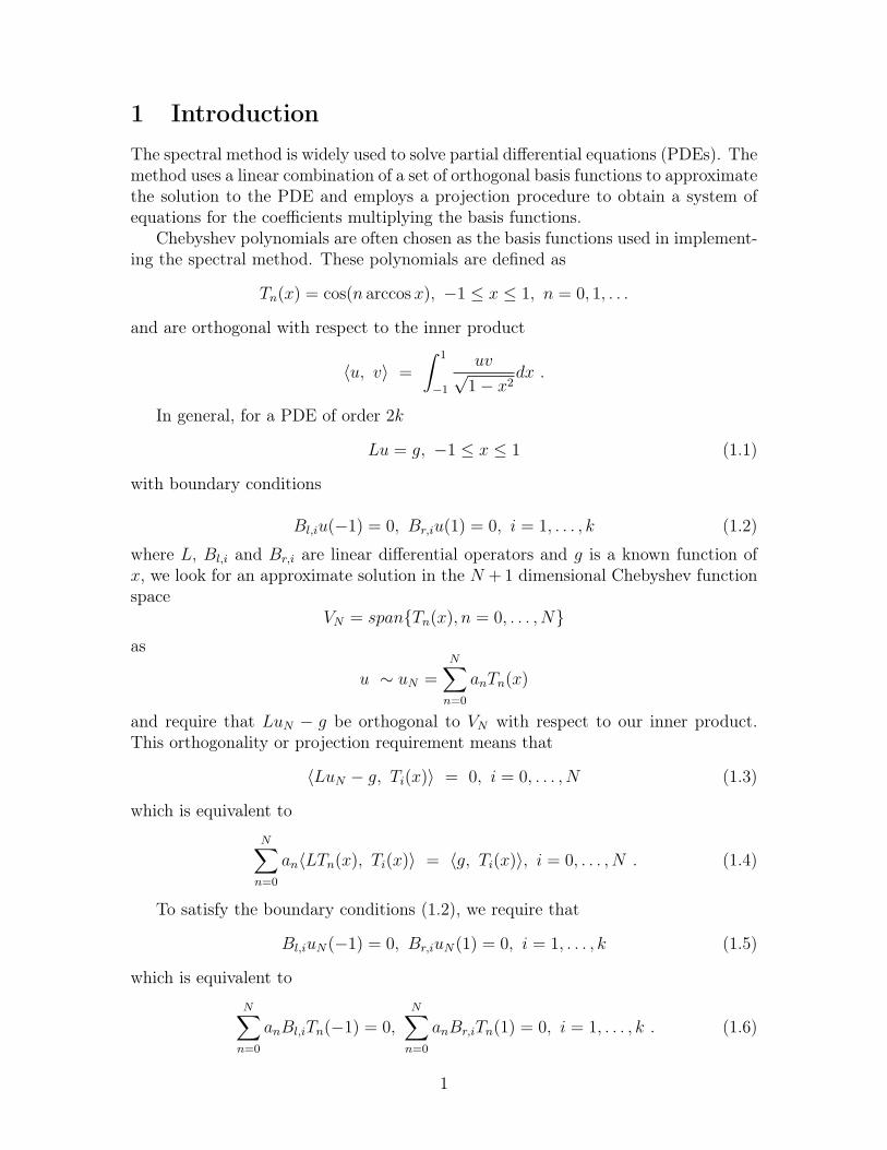
1 Introduction
The spectral method is widely used to solve partial differential equations (PDEs). Themethod uses a linear combination of a set of orthogonal basis functions to approximatethe solution to the PDE and employs a projection procedure to obtain a system ofequations for the coefficients multiplying the basis functions.
Chebyshev polynomials are often chosen as the basis functions used in implement-ing the spectral method. These polynomials are defined as
Tn(x) = cos(n arccos x), −1 ≤ x ≤ 1, n = 0, 1, . . .
and are orthogonal with respect to the inner product
〈u, v〉 =
∫ 1
−1
uv√1 − x2
dx .
In general, for a PDE of order 2k
Lu = g, −1 ≤ x ≤ 1 (1.1)
with boundary conditions
Bl,iu(−1) = 0, Br,iu(1) = 0, i = 1, . . . , k (1.2)
where L, Bl,i and Br,i are linear differential operators and g is a known function ofx, we look for an approximate solution in the N + 1 dimensional Chebyshev functionspace
VN = span{Tn(x), n = 0, . . . , N}as
u ∼ uN =N
∑
n=0
anTn(x)
and require that LuN − g be orthogonal to VN with respect to our inner product.This orthogonality or projection requirement means that
〈LuN − g, Ti(x)〉 = 0, i = 0, . . . , N (1.3)
which is equivalent to
N∑
n=0
an〈LTn(x), Ti(x)〉 = 〈g, Ti(x)〉, i = 0, . . . , N . (1.4)
To satisfy the boundary conditions (1.2), we require that
Bl,iuN(−1) = 0, Br,iuN(1) = 0, i = 1, . . . , k (1.5)
which is equivalent to
N∑
n=0
anBl,iTn(−1) = 0,N
∑
n=0
anBr,iTn(1) = 0, i = 1, . . . , k . (1.6)
1
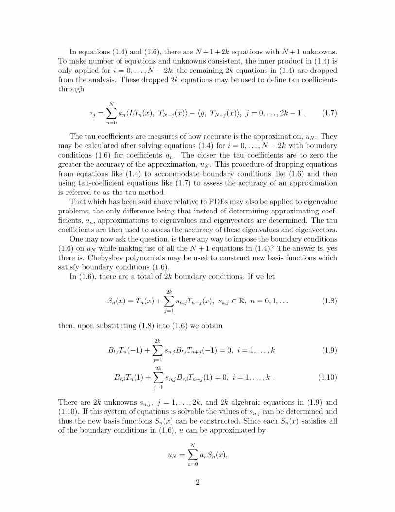
In equations (1.4) and (1.6), there are N +1+2k equations with N +1 unknowns.To make number of equations and unknowns consistent, the inner product in (1.4) isonly applied for i = 0, . . . , N − 2k; the remaining 2k equations in (1.4) are droppedfrom the analysis. These dropped 2k equations may be used to define tau coefficientsthrough
τj =N
∑
n=0
an〈LTn(x), TN−j(x)〉 − 〈g, TN−j(x)〉, j = 0, . . . , 2k − 1 . (1.7)
The tau coefficients are measures of how accurate is the approximation, uN . Theymay be calculated after solving equations (1.4) for i = 0, . . . , N − 2k with boundaryconditions (1.6) for coefficients an. The closer the tau coefficients are to zero thegreater the accuracy of the approximation, uN . This procedure of dropping equationsfrom equations like (1.4) to accommodate boundary conditions like (1.6) and thenusing tau-coefficient equations like (1.7) to assess the accuracy of an approximationis referred to as the tau method.
That which has been said above relative to PDEs may also be applied to eigenvalueproblems; the only difference being that instead of determining approximating coef-ficients, an, approximations to eigenvalues and eigenvectors are determined. The taucoefficients are then used to assess the accuracy of these eigenvalues and eigenvectors.
One may now ask the question, is there any way to impose the boundary conditions(1.6) on uN while making use of all the N + 1 equations in (1.4)? The answer is, yesthere is. Chebyshev polynomials may be used to construct new basis functions whichsatisfy boundary conditions (1.6).
In (1.6), there are a total of 2k boundary conditions. If we let
Sn(x) = Tn(x) +2k
∑
j=1
sn,jTn+j(x), sn,j ∈ R, n = 0, 1, . . . (1.8)
then, upon substituting (1.8) into (1.6) we obtain
Bl,iTn(−1) +2k
∑
j=1
sn,jBl,iTn+j(−1) = 0, i = 1, . . . , k (1.9)
Br,iTn(1) +2k
∑
j=1
sn,jBr,iTn+j(1) = 0, i = 1, . . . , k . (1.10)
There are 2k unknowns sn,j, j = 1, . . . , 2k, and 2k algebraic equations in (1.9) and(1.10). If this system of equations is solvable the values of sn,j can be determined andthus the new basis functions Sn(x) can be constructed. Since each Sn(x) satisfies allof the boundary conditions in (1.6), u can be approximated by
uN =N
∑
n=0
anSn(x),
2
and (1.4) can be solved directly as
N∑
n=0
an
(
〈LTn(x), Ti(x)〉 +2k
∑
j=1
sn,j〈LTn+j(x), Ti(x)〉)
= 〈g, Ti(x)〉, i = 0, . . . , N .
(1.11)
2 Notation and Formulae
For convenience, we introduce some notation. Suppose
f(x) =N
∑
i=0
fiTi(x) = fT TN
where
f =
f0...
fN
, TN =
T0(x)...
TN(x)
and fT denotes the transpose of f .From now on, f(x) = fT TN is denoted as
f(x)VN−→ f
where VN is the Chebyshev function space defined in Section 1. This notation meansthat f(x) may be expanded in the function space VN as the vector f . Furthermore,using properties of Chebyshev polynomials, it can be shown that
f(x)VN−→ f ⇒ dk
dxkf(x)
VN−→ M kf , k ≥ 1 (2.1)
where the matrix, M is of order (N + 1) × (N + 1) and is defined in Appendix A.Now let
g(x)VN−→ g =
g0...
gN
.
Then, using the multiplication law,
Ti(x)Tj(x) =1
2Ti+j(x) +
1
2T|i−j|(x)
3
for Chebyshev polynomials the product f(x)g(x) may be approximated as,
f(x)g(x) =N
∑
i=0
fiTi(x)N
∑
j=0
gjTj(x)
=N
∑
i=0
N∑
j=0
figjTi(x)Tj(x)
=1
2
N∑
i=0
N∑
j=0
figj
[
Ti+j(x) + T|i−j|(x)]
=1
2
2N∑
i=0
S1,iTi(x) +1
2
N∑
i=0
S2,iTi(x)
where
S1,i =∑
p+q=i0≤p,q≤N
fpgq, 0 ≤ i ≤ 2N (2.2)
and
S2,i =∑
|p−q|=i0≤p,q≤N
fpgq, 0 ≤ i ≤ N . (2.3)
From (2.2) we have that
S1,0 = f0g0
S1,1 = f0g1 + f1g0
S1,2 = f0g2 + f1g1 + f2g0
...
S1,N = f0gN + f1gN−1 + . . . + fNg0
and thus that
S1,0
S1,1...
S1,N
=
f0
f1 f0...
fN fN−1 . . . f1 f0
g0......
gN
≡ W1 g .
Likewise, from (2.3) we have that
S2,0 = f0g0 + f1g1 + . . . + fNgN
S2,1 = f0g1 + f1g2 + . . . + fN−1gN
+f1g0 + f2g1 + . . . + fNgN−1
...
S2,N = f0gN + fNg0
4
and thus that
S2,0
S2,1...
S2,N
=
f0 f1 f2 . . . fN−1 fN
f1 f0 + f1 f1 + f2 . . . fN−2 + fN fN−1...
fN 0 . . . 0 f0
g0......
gN
≡ W2 g .
Thus, we get that
f(x)g(x) =1
2
2N∑
i=0
S1,iTi(x) +1
2
N∑
i=0
S2,iTi(x)
=1
2
N∑
i=0
S1,iTi(x) +1
2
N∑
i=0
S2,iTi(x) +1
2
2N∑
i=N+1
S1,iTi(x)
=1
2[W1 g]T TN +
1
2[W2 g]T TN +
1
2[W3 g]T T ∗
N
=
[
1
2(W1 + W2)g
]T
TN +
[
1
2W3 g
]T
T ∗N
where
T ∗N =
TN+1(x)...
T2N(x)
.
If we let Wf = 12(W1 + W2), and W ∗
f = 12W3, then
f(x)g(x) = [Wf g]T TN +[
W ∗f g
]TT ∗
N (2.4)
where W ∗f is not given explicitly because it consists of only terms of order higher
than N , which become zero after applying inner product with Tk(x), k = 0, 1, . . . , N .
3 Beam Equations
We are given the following system of partial differential equations describing themotion of two coupled beams
∂2u1
∂t2= −p1
∂4u1
∂x4− k(x) (u1 − u2) − δk(x)
∂u1
∂t(3.1a)
∂2u2
∂t2= −p2
∂4u2
∂x4+ k(x) (u1 − u2) − δk(x)
∂u2
∂t(3.1b)
5
with boundary conditions
∂2u1
∂x2(t,−1) =
∂2u1
∂x2(t, 1) = 0 (3.2a)
∂3u1
∂x3(t,−1) =
∂3u1
∂x3(t, 1) = 0 (3.2b)
u2(t,−1) = u2(t, 1) = 0 (3.2c)
∂u2
∂x(t,−1) =
∂u2
∂x(t, 1) = 0 (3.2d)
where p1 > 0, p2 > 0, and δ ≥ 0 are given parameters and k(x) is a known function.If we introduce the substitutions, v1 = ∂u1
∂tand v2 = ∂u2
∂t, the original equations
(3.1a) and (3.1b) become
∂u1
∂t= v1 (3.3a)
∂v1
∂t= −p1
∂4u1
∂x4− k(x)(u1 − u2) − δk(x)v1 (3.3b)
∂u2
∂t= v2 (3.3c)
∂v2
∂t= −p2
∂4u2
∂x4+ k(x)(u1 − u2) − δk(x)v2. (3.3d)
Section 3.1 describes how to apply the Tau method to the above equations, section3.2 describes how to construct new basis functions to solve the above equations, andsection 4 compares the numerical results given by these two techniques.
3.1 The Tau Method
To develop the discretized system of equations associated with the tau method, wefirst expand the variables appearing in equations (3.3a) - (3.3d) in the function spaceVN as,
u1VN−→ a(t) =
a0(t)...
aN(t)
⇒
{
∂u1
∂t
VN−→ a(t)∂4u1
∂x4
VN−→ M 4a(t)
u2VN−→ b(t) =
b0(t)...
bN(t)
⇒
{
∂u2
∂t
VN−→ b(t)∂4u2
∂x4
VN−→ M 4b(t)
v1VN−→ c(t) =
c0(t)...
cN(t)
⇒ ∂v1
∂t
VN−→ c(t)
6

v2VN−→ d(t) =
d0(t)...
dN(t)
⇒ ∂v2
∂t
VN−→ d(t)
and
k(x)VN−→ k =
k0...
kN
,
where the superposed dot denotes time differentiation.
Next, for an arbitrary vector r(t) in VN , we introduce the partitioning:
r(t) =
[
rf (t)rl(t)
]
, rf (t) =
r0(t)...
rN−4(t)
, rl(t) =
rN−3(t)...
rN(t)
(3.4)
and define the vectors R1 and R−1 through
R1 =
T0(1)T1(1)
...TN(1)
, R−1 =
T0(−1)T1(−1)
...TN(−1)
.
The above definitions, partitioning and function space expansions are next appliedto the boundary conditions, (3.2a) - (3.2d). Using the expansion for u1 and the vectorsR1 and R−1, we write the boundary conditions, (3.2a)-(3.2b), as
[
M 2a(t)]T
R−1 = 0 ⇒ [a(t)]T[
M 2]T
R−1 = 0 ≡ [a(t)]T S1 = 0[
M 2a(t)]T
R1 = 0 ⇒ [a(t)]T[
M 2]T
R1 = 0 ≡ [a(t)]T S2 = 0[
M 3a(t)]T
R−1 = 0 ⇒ [a(t)]T[
M 3]T
R−1 = 0 ≡ [a(t)]T S3 = 0[
M 3a(t)]T
R1 = 0 ⇒ [a(t)]T[
M 3]T
R1 = 0 ≡ [a(t)]T S4 = 0 , (3.5)
where S1 and S3 are respectively, [M 2]T
and [M 3]T
applied to R−1 and S2 and S4
are respectively, [M 2]T
and [M 3]T
applied to R1. Using the partitioning of (3.4), wecan write equation (3.5) in partitioned form as,
[
[af (t)]T
, [al(t)]T]
[
S1,f S2,f S3,f S4,f
S1,l S2,l S3,l S4,l
]
= 0
or, alternatively as[af (t)]
TP1 + [al(t)]
TP2 = 0 (3.6)
where P1 =[
S1,f S2,f S3,f S4,f
]
and P2 =[
S1,l S2,l S3,l S4,l
]
. AssumingP2 is invertible, we can solve (3.6) for al(t),
7

al(t) = −[
P1P−12
]Taf (t). (3.7)
As in the development above that led to equations (3.6) and (3.7), we now usethe expansion for u2 and write the boundary conditions, (3.2c)-(3.2d), as
[b(t)]T R−1 = 0 ≡ [b(t)]T S5 = 0
[b(t)]T R1 = 0 ≡ [b(t)]T S6 = 0
[Mb(t)]T R−1 = 0 ⇒ [b(t)]T MT R−1 = 0 ≡ [b(t)]T S7 = 0
[Mb(t)]T R1 = 0 ⇒ [b(t)]T MT R1 = 0 ≡ [b(t)]T S8 = 0 (3.8)
which may be written in partitioned form as
[
[bf (t)]T
, [bl(t)]T]
[
S5,f S6,f S7,f S8,f
S5,l S6,l S7,l S8,l
]
= 0
or, alternatively as[bf (t)]
TP3 + [bl(t)]
TP4 = 0 (3.9)
where P3 =[
S5,f S6,f S7,f S8,f
]
and P4 =[
S5,l S6,l S7,l S8,l
]
. AssumingP4 is invertible, we can solve (3.9) for bl(t),
bl(t) = −[
P3P−14
]Tbf (t). (3.10)
We note that P1 and P3 are of order (N − 3) × 4 and that P2 and P4 are of order4 × 4.
From (3.7) and (3.10), we see that
al(t) = −[
P1P−12
]Taf (t) (3.11)
andbl(t) = −
[
P3P−14
]Tbf (t). (3.12)
Furthermore, using equations (3.7) and (3.10), we may eliminate the last fourelements from the vectors a(t) and b(t) and represent those vectors as
a(t) =
[
IN−3
−[
P1P−12
]T
]
af (t) ≡ C1af (t) (3.13)
b(t) =
[
IN−3
−[
P3P−14
]T
]
bf (t) ≡ C2bf (t), (3.14)
where the partitioned matrices C1 and C2 are of order (N + 1) × (N − 3) and IN−3
denotes the (N − 3) × (N − 3) identity matrix. Thus far we have discretized andaccounted for the boundary conditions, (3.2a) - (3.2d).
The next step in obtaining the system of equations associated with the tau methodis to discretize the system of differential equations, (3.3a) - (3.3d). Using the functionspace expansions for u1 and v1 in VN , we obtain from equation (3.3a) that,
[a(t)]T TN = [c(t)]T TN .
8

Upon taking the inner product of the above with Ti(x), i = 0, . . . , N , we get that,
ai(t) = ci(t), i = 0, . . . , N,
and thus, with the partitioning of (3.4), that
af (t) = cf (t) (3.15)
andal(t) = cl(t). (3.16)
Equations (3.15) and (3.16) with equation (3.11) imply that
cl(t) = −[
P1P−12
]Tcf (t)
and hence, as in equation (3.13), that
c(t) = C1cf (t). (3.17)
Similarly, upon using the function space expansions for u2 and v2 in VN , we obtainfrom (3.3c), that
bf (t) = df (t) (3.18)
andbl(t) = dl(t) (3.19)
and thus, with equation (3.12), that
dl(t) = −[
P3P−14
]Tdf (t).
Hence, as in equation (3.14), we get that
d(t) = C2df (t). (3.20)
Equation (3.17) means that v1 must satisfy the same boundary conditions, (3.2a)-(3.2b), as u1 and equation (3.20) means that v2 must satisfy the same boundaryconditions, (3.2c)-(3.2d), as u2. In fact, if u1 and u2 are sufficiently smooth, then itcan be shown from (3.3a) and (3.3c) that
∂2v1
∂x2(t,±1) =
∂2
∂x2
∂u1
∂t(t,±1) =
∂
∂t
∂2u1
∂x2(t,±1) = 0 (3.21)
∂3v1
∂x3(t,±1) =
∂3
∂x3
∂u1
∂t(t,±1) =
∂
∂t
∂3u1
∂x3(t,±1) = 0 (3.22)
v2(t,±1) =∂u2
∂t(t,±1) = 0 (3.23)
∂v2
∂x(t,±1) =
∂
∂x
∂u2
∂t(t,±1) =
∂
∂t
∂u2
∂x(t,±1) = 0. (3.24)
which are the same conditions as (3.2a) - (3.2d), but for v1 and v2.
9
The remaining equations to be discretized are equations (3.3b) and (3.3d). Using(2.4) for functions expanded in the function space, VN we get that
k(x)u1 = [Wk a(t)]T TN + [W ∗k a(t)]T T ∗
N
k(x)u2 = [Wk b(t)]T TN + [W ∗k b(t)]T T ∗
N
k(x)v1 = [Wk c(t)]T TN + [W ∗k c(t)]T T ∗
N
k(x)v2 = [Wk d(t)]T TN + [W ∗k d(t)]T T ∗
N .
With the function space expansion of u1, u2 and v1 in VN , we then obtain from(3.3b) that,
[c(t)]T TN = −p1
[
M 4a(t)]T
TN − [Wk a(t)]T TN − [W ∗k a(t)]T T ∗
N
+ [Wk b(t)]T TN + [W ∗k b(t)]T T ∗
N
−δ [Wk c(t)]T TN − δ [W ∗k c(t)]T T ∗
N
Upon taking the inner product of the above with Ti(x), i = 0, . . . , N − 4, we get that
ci(t) =[
−p1M4]
ia(t) − [Wk]i a(t) + [Wk]i b(t) − δ [Wk]i c(t), (3.25)
where [ ∗ ]i denotes the ith row of the indicated matrix.Equations (3.25) may be written in matrix-vector form as,
cf (t) = A1a(t) − Ba(t) + Bb(t) − δBc(t) (3.26)
where A1, of order (N − 3)× (N + 1), is the submatrix obtained from the first N − 3rows of −p1M
4 and B, of order (N − 3) × (N + 1), is the submatrix obtained fromthe first N − 3 rows of Wk.
Using equations (3.13), (3.14) and (3.17), we may simplify equation (3.26) as
cf (t) = (A1 − B)C1af (t) + BC2bf (t) − δBC1cf (t), (3.27)
where only the first N − 3 elements of vectors appear as unknowns.Similarly, by substituting the function space expansion for u1, u2 and v2 into
equation (3.3d), taking the inner product of the resulting equation with Ti(x), i =0, . . . , N − 4 and using equations (3.13), (3.14) and (3.20), we may deduce that
df (t) = BC1af (t) + (A2 − B)C2bf (t) − δBC2df (t), (3.28)
where A2, of order (N − 3)× (N + 1), is the submatrix obtained from the first N − 3rows of −p2M
4.If we now let
z(t) =
af (t)bf (t)cf (t)df (t)
10
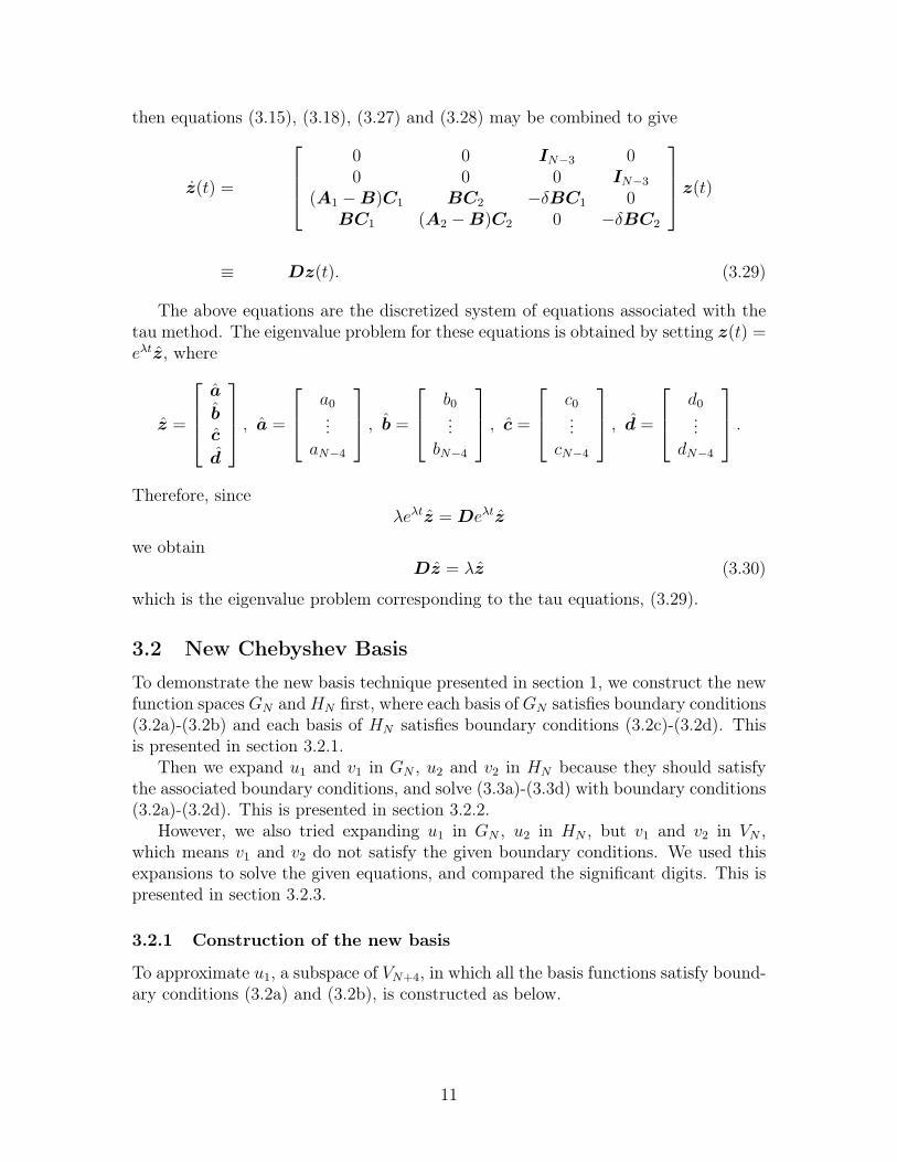
then equations (3.15), (3.18), (3.27) and (3.28) may be combined to give
z(t) =
0 0 IN−3 00 0 0 IN−3
(A1 − B)C1 BC2 −δBC1 0BC1 (A2 − B)C2 0 −δBC2
z(t)
≡ Dz(t). (3.29)
The above equations are the discretized system of equations associated with thetau method. The eigenvalue problem for these equations is obtained by setting z(t) =eλtz, where
z =
a
b
c
d
, a =
a0...
aN−4
, b =
b0...
bN−4
, c =
c0...
cN−4
, d =
d0...
dN−4
.
Therefore, sinceλeλtz = Deλtz
we obtainDz = λz (3.30)
which is the eigenvalue problem corresponding to the tau equations, (3.29).
3.2 New Chebyshev Basis
To demonstrate the new basis technique presented in section 1, we construct the newfunction spaces GN and HN first, where each basis of GN satisfies boundary conditions(3.2a)-(3.2b) and each basis of HN satisfies boundary conditions (3.2c)-(3.2d). Thisis presented in section 3.2.1.
Then we expand u1 and v1 in GN , u2 and v2 in HN because they should satisfythe associated boundary conditions, and solve (3.3a)-(3.3d) with boundary conditions(3.2a)-(3.2d). This is presented in section 3.2.2.
However, we also tried expanding u1 in GN , u2 in HN , but v1 and v2 in VN ,which means v1 and v2 do not satisfy the given boundary conditions. We used thisexpansions to solve the given equations, and compared the significant digits. This ispresented in section 3.2.3.
3.2.1 Construction of the new basis
To approximate u1, a subspace of VN+4, in which all the basis functions satisfy bound-ary conditions (3.2a) and (3.2b), is constructed as below.
11
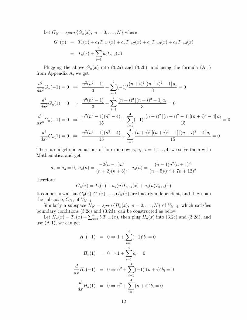
Let GN = span {Gn(x), n = 0, . . . , N} where
Gn(x) = Tn(x) + a1Tn+1(x) + a2Tn+2(x) + a3Tn+3(x) + a4Tn+4(x)
= Tn(x) +4
∑
i=1
aiTn+i(x)
Plugging the above Gn(x) into (3.2a) and (3.2b), and using the formula (A.1)from Appendix A, we get
d2
dx2Gn(−1) = 0 ⇒ n2(n2 − 1)
3+
4∑
i=1
(−1)i (n + i)2 [(n + i)2 − 1] ai
3= 0
d2
dx2Gn(1) = 0 ⇒ n2(n2 − 1)
3+
4∑
i=1
(n + i)2 [(n + i)2 − 1] ai
3= 0
d3
dx3Gn(−1) = 0 ⇒ n2(n2 − 1)(n2 − 4)
15+
4∑
i=1
(−1)i (n + i)2 [(n + i)2 − 1] [(n + i)2 − 4] ai
15= 0
d3
dx3Gn(1) = 0 ⇒ n2(n2 − 1)(n2 − 4)
15+
4∑
i=1
(n + i)2 [(n + i)2 − 1] [(n + i)2 − 4] ai
15= 0
These are algebraic equations of four unknowns, ai, i = 1, . . . , 4, we solve them withMathematica and get
a1 = a3 = 0, a2(n) =−2(n − 1)n2
(n + 2)(n + 3)2, a4(n) =
(n − 1)n2(n + 1)2
(n + 5)(n2 + 7n + 12)2
thereforeGn(x) = Tn(x) + a2(n)Tn+2(x) + a4(n)Tn+4(x)
It can be shown that G0(x), G1(x), . . . , GN(x) are linearly independent, and they spanthe subspace, GN , of VN+4.
Similarly a subspace HN = span {Hn(x), n = 0, . . . , N} of VN+4, which satisfiesboundary conditions (3.2c) and (3.2d), can be constructed as below.
Let Hn(x) = Tn(x) +∑4
i=1 biTn+i(x), then plug Hn(x) into (3.2c) and (3.2d), anduse (A.1), we can get
Hn(−1) = 0 ⇒ 1 +4
∑
i=1
(−1)ibi = 0
Hn(1) = 0 ⇒ 1 +4
∑
i=1
bi = 0
d
dxHn(−1) = 0 ⇒ n2 +
4∑
i=1
(−1)i(n + i)2bi = 0
d
dxHn(1) = 0 ⇒ n2 +
4∑
i=1
(n + i)2bi = 0
12
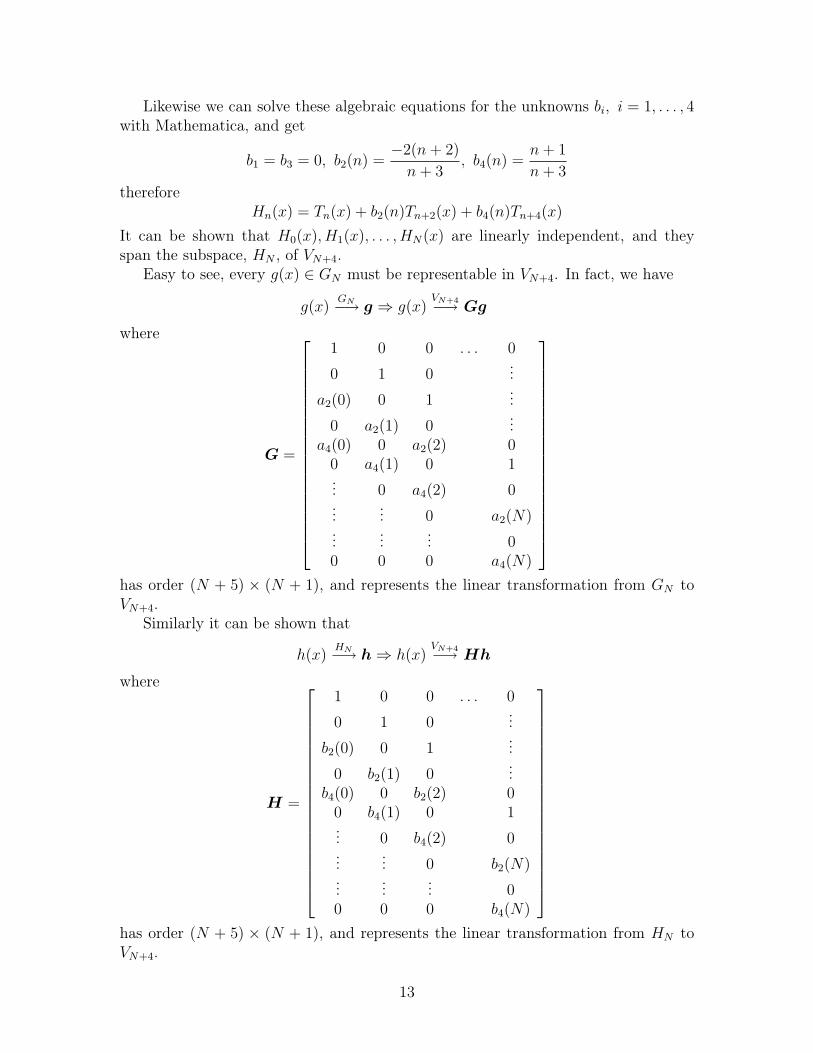
Likewise we can solve these algebraic equations for the unknowns bi, i = 1, . . . , 4with Mathematica, and get
b1 = b3 = 0, b2(n) =−2(n + 2)
n + 3, b4(n) =
n + 1
n + 3
thereforeHn(x) = Tn(x) + b2(n)Tn+2(x) + b4(n)Tn+4(x)
It can be shown that H0(x), H1(x), . . . , HN(x) are linearly independent, and theyspan the subspace, HN , of VN+4.
Easy to see, every g(x) ∈ GN must be representable in VN+4. In fact, we have
g(x)GN−→ g ⇒ g(x)
VN+4−→ Gg
where
G =
1 0 0 . . . 0
0 1 0...
a2(0) 0 1...
0 a2(1) 0...
a4(0) 0 a2(2) 00 a4(1) 0 1... 0 a4(2) 0...
... 0 a2(N)...
...... 0
0 0 0 a4(N)
has order (N + 5) × (N + 1), and represents the linear transformation from GN toVN+4.
Similarly it can be shown that
h(x)HN−→ h ⇒ h(x)
VN+4−→ Hh
where
H =
1 0 0 . . . 0
0 1 0...
b2(0) 0 1...
0 b2(1) 0...
b4(0) 0 b2(2) 00 b4(1) 0 1... 0 b4(2) 0...
... 0 b2(N)...
...... 0
0 0 0 b4(N)
has order (N + 5) × (N + 1), and represents the linear transformation from HN toVN+4.
13
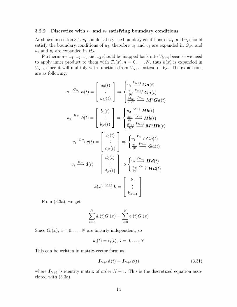
3.2.2 Discretize with v1 and v2 satisfying boundary conditions
As shown in section 3.1, v1 should satisfy the boundary conditions of u1, and v2 shouldsatisfy the boundary conditions of u2, therefore u1 and v1 are expanded in GN , andu2 and v2 are expanded in HN .
Furthermore, u1, u2, v1 and v2 should be mapped back into VN+4 because we needto apply inner product to them with Tn(x), n = 0, . . . , N , thus k(x) is expanded inVN+4 since it will multiply with functions from VN+4 instead of VN . The expansionsare as following.
u1GN−→ a(t) =
a0(t)...
aN(t)
⇒
u1VN+4−→ Ga(t)
∂u1
∂t
VN+4−→ Ga(t)∂4u1
∂x4
VN+4−→ M 4Ga(t)
u2HN−→ b(t) =
b0(t)...
bN(t)
⇒
u2VN+4−→ Hb(t)
∂u2
∂t
VN+4−→ Hb(t)∂4u2
∂x4
VN+4−→ M 4Hb(t)
v1GN−→ c(t) =
c0(t)...
cN(t)
⇒
{
v1VN+4−→ Gc(t)
∂v1
∂t
VN+4−→ Gc(t)
v2HN−→ d(t) =
d0(t)...
dN(t)
⇒
{
v2VN+4−→ Hd(t)
∂v2
∂t
VN+4−→ Hd(t)
k(x)VN+4−→ k =
k0...
kN+4
From (3.3a), we get
N∑
i=0
ai(t)Gi(x) =N
∑
i=0
ci(t)Gi(x)
Since Gi(x), i = 0, . . . , N are linearly independent, so
ai(t) = ci(t), i = 0, . . . , N
This can be written in matrix-vector form as
IN+1a(t) = IN+1c(t) (3.31)
where IN+1 is identity matrix of order N + 1. This is the discretized equation asso-ciated with (3.3a).
14
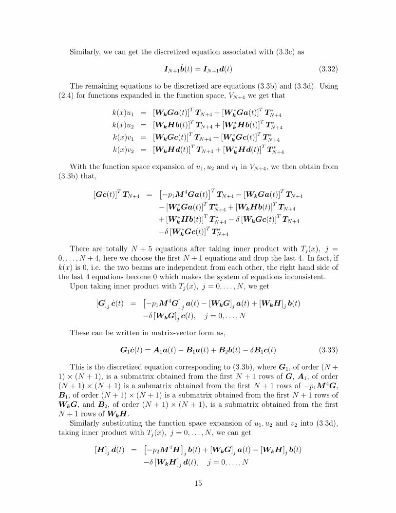
Similarly, we can get the discretized equation associated with (3.3c) as
IN+1b(t) = IN+1d(t) (3.32)
The remaining equations to be discretized are equations (3.3b) and (3.3d). Using(2.4) for functions expanded in the function space, VN+4 we get that
k(x)u1 = [WkGa(t)]T TN+4 + [W ∗kGa(t)]T T ∗
N+4
k(x)u2 = [WkHb(t)]T TN+4 + [W ∗kHb(t)]T T ∗
N+4
k(x)v1 = [WkGc(t)]T TN+4 + [W ∗kGc(t)]T T ∗
N+4
k(x)v2 = [WkHd(t)]T TN+4 + [W ∗kHd(t)]T T ∗
N+4
With the function space expansion of u1, u2 and v1 in VN+4, we then obtain from(3.3b) that,
[Gc(t)]T TN+4 =[
−p1M4Ga(t)
]TTN+4 − [WkGa(t)]T TN+4
− [W ∗kGa(t)]T T ∗
N+4 + [WkHb(t)]T TN+4
+ [W ∗kHb(t)]T T ∗
N+4 − δ [WkGc(t)]T TN+4
−δ [W ∗kGc(t)]T T ∗
N+4
There are totally N + 5 equations after taking inner product with Tj(x), j =0, . . . , N + 4, here we choose the first N + 1 equations and drop the last 4. In fact, ifk(x) is 0, i.e. the two beams are independent from each other, the right hand side ofthe last 4 equations become 0 which makes the system of equations inconsistent.
Upon taking inner product with Tj(x), j = 0, . . . , N , we get
[G]j c(t) =[
−p1M4G
]
ja(t) − [WkG]j a(t) + [WkH ]j b(t)
−δ [WkG]j c(t), j = 0, . . . , N
These can be written in matrix-vector form as,
G1c(t) = A1a(t) − B1a(t) + B2b(t) − δB1c(t) (3.33)
This is the discretized equation corresponding to (3.3b), where G1, of order (N +1) × (N + 1), is a submatrix obtained from the first N + 1 rows of G, A1, of order(N + 1) × (N + 1) is a submatrix obtained from the first N + 1 rows of −p1M
4G,B1, of order (N + 1) × (N + 1) is a submatrix obtained from the first N + 1 rows ofWkG, and B2, of order (N + 1) × (N + 1), is a submatrix obtained from the firstN + 1 rows of WkH .
Similarly substituting the function space expansion of u1, u2 and v2 into (3.3d),taking inner product with Tj(x), j = 0, . . . , N , we can get
[H ]j d(t) =[
−p2M4H
]
jb(t) + [WkG]j a(t) − [WkH ]j b(t)
−δ [WkH ]j d(t), j = 0, . . . , N
15
These can be written in matrix-vector form as,
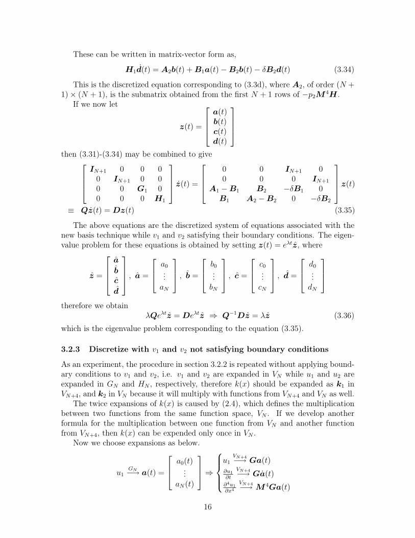
H1d(t) = A2b(t) + B1a(t) − B2b(t) − δB2d(t) (3.34)
This is the discretized equation corresponding to (3.3d), where A2, of order (N +1) × (N + 1), is the submatrix obtained from the first N + 1 rows of −p2M
4H .If we now let
z(t) =
a(t)b(t)c(t)d(t)
then (3.31)-(3.34) may be combined to give
IN+1 0 0 00 IN+1 0 00 0 G1 00 0 0 H1
z(t) =
0 0 IN+1 00 0 0 IN+1
A1 − B1 B2 −δB1 0B1 A2 − B2 0 −δB2
z(t)
≡ Qz(t) = Dz(t) (3.35)
The above equations are the discretized system of equations associated with thenew basis technique while v1 and v2 satisfying their boundary conditions. The eigen-value problem for these equations is obtained by setting z(t) = eλtz, where
z =
a
b
c
d
, a =
a0...
aN
, b =
b0...
bN
, c =
c0...
cN
, d =
d0...
dN
therefore we obtainλQeλtz = Deλtz ⇒ Q−1Dz = λz (3.36)
which is the eigenvalue problem corresponding to the equation (3.35).
3.2.3 Discretize with v1 and v2 not satisfying boundary conditions
As an experiment, the procedure in section 3.2.2 is repeated without applying bound-ary conditions to v1 and v2, i.e. v1 and v2 are expanded in VN while u1 and u2 areexpanded in GN and HN , respectively, therefore k(x) should be expanded as k1 inVN+4, and k2 in VN because it will multiply with functions from VN+4 and VN as well.
The twice expansions of k(x) is caused by (2.4), which defines the multiplicationbetween two functions from the same function space, VN . If we develop anotherformula for the multiplication between one function from VN and another functionfrom VN+4, then k(x) can be expended only once in VN .
Now we choose expansions as below.
u1GN−→ a(t) =
a0(t)...
aN(t)
⇒
u1VN+4−→ Ga(t)
∂u1
∂t
VN+4−→ Ga(t)∂4u1
∂x4
VN+4−→ M 4Ga(t)
16

u2HN−→ b(t) =
b0(t)...
bN(t)
⇒
u2VN+4−→ Hb(t)
∂u2
∂t
VN+4−→ Hb(t)∂4u2
∂x4
VN+4−→ M 4Hb(t)
v1VN−→ c(t) =
c0(t)...
cN(t)
⇒ ∂v1
∂t
VN−→ c(t)
v2VN−→ d(t) =
d0(t)...
dN(t)
⇒ ∂v2
∂t
VN−→ d(t)
k(x)VN+4−→ k1 =
k1,0...
k1,N+4
k(x)VN−→ k2 =
k2,0...
k2,N
From (3.3a), we get[Ga(t)]T TN+4 = [c(t)]T TN
After taking inner product with Tj(x), j = 0, . . . , N , we get
[G]j a(t) = cj(t), j = 0, . . . , N
where cj(t) denotes the jth component of c(t), [G]j is the jth row of G. Writing themin matrix-vector form yields
G1a(t) = IN+1c(t) (3.37)
where G1, of order (N + 1) × (N + 1), is a submatrix obtained from the first N + 1rows of G, and IN+1 is identity matrix of order N + 1.
Similarly from (3.3c), it can be shown that
H1b(t) = IN+1d(t) (3.38)
where H1, of order (N + 1) × (N + 1), is a submatrix obtained from the first N + 1rows of H .
The remaining equations to be discretized are equations (3.3b) and (3.3d). Using(2.4) for functions expanded in the function spaces, VN and VN+4 we get that
k(x)u1 = [Wk1Ga(t)]T TN+4 +
[
W ∗k1
Ga(t)]T
T ∗N+4
k(x)u2 = [Wk1Hb(t)]T TN+4 +
[
W ∗k1
Hb(t)]T
T ∗N+4
k(x)v1 = [Wk2c(t)]T TN +
[
W ∗k2
c(t)]T
T ∗N
k(x)v2 = [Wk2d(t)]T TN +
[
W ∗k2
d(t)]T
T ∗N
17
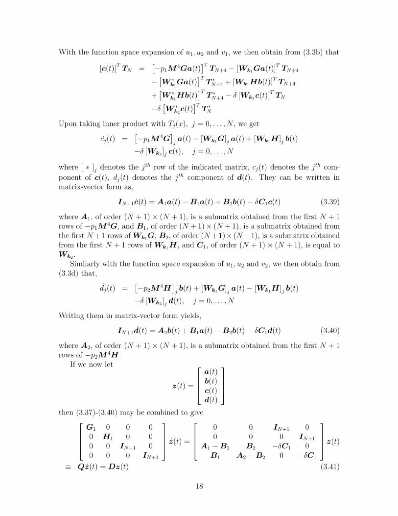
With the function space expansion of u1, u2 and v1, we then obtain from (3.3b) that
[c(t)]T TN =[
−p1M4Ga(t)
]TTN+4 − [Wk1
Ga(t)]T TN+4
−[
W ∗k1
Ga(t)]T
T ∗N+4 + [Wk1
Hb(t)]T TN+4
+[
W ∗k1
Hb(t)]T
T ∗N+4 − δ [Wk2
c(t)]T TN
−δ[
W ∗k2
c(t)]T
T ∗N
Upon taking inner product with Tj(x), j = 0, . . . , N , we get
cj(t) =[
−p1M4G
]
ja(t) − [Wk1
G]j a(t) + [Wk1H ]j b(t)
−δ [Wk2]j c(t), j = 0, . . . , N
where [ ∗ ]j denotes the jth row of the indicated matrix, cj(t) denotes the jth com-
ponent of c(t), dj(t) denotes the jth component of d(t). They can be written inmatrix-vector form as,
IN+1c(t) = A1a(t) − B1a(t) + B2b(t) − δC1c(t) (3.39)
where A1, of order (N + 1) × (N + 1), is a submatrix obtained from the first N + 1rows of −p1M
4G, and B1, of order (N + 1)× (N + 1), is a submatrix obtained fromthe first N +1 rows of Wk1
G, B2, of order (N +1)× (N +1), is a submatrix obtainedfrom the first N + 1 rows of Wk1
H , and C1, of order (N + 1) × (N + 1), is equal toWk2
.Similarly with the function space expansion of u1, u2 and v2, we then obtain from
(3.3d) that,
dj(t) =[
−p2M4H
]
jb(t) + [Wk1
G]j a(t) − [Wk1H ]j b(t)
−δ [Wk2]j d(t), j = 0, . . . , N
Writing them in matrix-vector form yields,
IN+1d(t) = A2b(t) + B1a(t) − B2b(t) − δC1d(t) (3.40)
where A2, of order (N + 1) × (N + 1), is a submatrix obtained from the first N + 1rows of −p2M
4H .If we now let
z(t) =
a(t)b(t)c(t)d(t)
then (3.37)-(3.40) may be combined to give
G1 0 0 00 H1 0 00 0 IN+1 00 0 0 IN+1
z(t) =
0 0 IN+1 00 0 0 IN+1
A1 − B1 B2 −δC1 0B1 A2 − B2 0 −δC1
z(t)
≡ Qz(t) = Dz(t) (3.41)
18
The above equations are the discretized system of equations associated with thenew basis technique while v1 and v2 not satisfying the boundary conditions. Theeigenvalue problem for these equations is obtained by setting z(t) = eλtz, where
z =
a
b
c
d
, a =
a0...
aN
, b =
b0...
bN
, c =
c0...
cN
, d =
d0...
dN
therefore we obtainQλeλtz = Deλtz ⇒ Q−1Dz = λz (3.42)
which is the eigenvalue problem corresponding to equation (3.41).
4 Numerical result
All the numerical experiments for equations (3.30), (3.36) and (3.42) are done withMatlab 7.9.0.529(64-bit) on a PC with Windows 7, and Q−1D is computed throughQ \ D, which, according to the Matlab documentations, provides better accuracythan Q−1D.
4.1 Separated problem
Consider the simplest case of p1 = p2 = 1, k(x) = 0 and δ = 0, then (3.3a)-(3.3d)become
∂u1
∂t= v1 (4.1)
∂v1
∂t= −∂4u1
∂x4(4.2)
with boundary conditions (3.2a)-(3.2b), and
∂u2
∂t= v2 (4.3)
∂v2
∂t= −∂4u2
∂x4(4.4)
with boundary conditions (3.2c)-(3.2d).They are actually the same equations but with different boundary conditions,
and analytically solvable, it can be shown that they have exactly the same solutionexcept that the boundary conditions (3.2a)-(3.2b) cause to 4 zero eigenvalues. Thefirst non-zero eigenvalue computed with Mathematica 7.0.0(64-bit) is exactly 0 +5.5933213620153309807i.
To do the computation, notice that k(x) = 0 and δ = 0, after plugging them into(3.30), (3.36) and (3.42), B in (3.30) becomes 0, B1 and B2 in (3.36) become 0, B1
19

and B2 in (3.42) become 0, therefore each of (3.30), (3.36) and (3.42) can be dividedfor the corresponding separated problem. For example, in (3.42), we define
Q1 =
[
IN+1 00 G1
]
, Q2 =
[
IN+1 0,0 H1
]
D1 =
[
0 IN+1
A1 0
]
, D2 =
[
0 IN+1
A2 0
]
The eigenvalue problem associated with (4.1)-(4.2) with boundary conditions (3.2a)-(3.2b) is
Q1−1D1z = λz
and the eigenvalue problem associated with (4.3)-(4.4) with boundary conditions(3.2c)-(3.2d) is
Q2−1D2z = λz
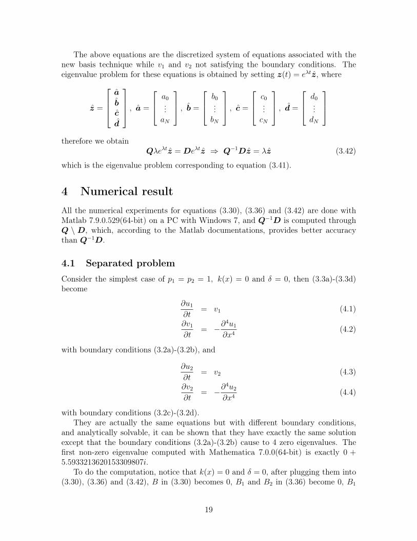
Table (4.1), (4.2) and (4.3) list the first non-zero eigenvalue given by (3.30), (3.36)and (3.42) when using boundary condition (3.2a)-(3.2b), respectively. Table (4.4),(4.5) and (4.6) list the first non-zero eigenvalue given by (3.30), (3.36) and (3.42)when using boundary condition (3.2c)-(3.2d), respectively.
As shown in the tables (4.1)-(4.3), the significant digits in imaginary part of theresult given by (3.30) get lost rapidly, but (3.36) and (3.42) can always give at least10 and 12 significant digits, respectively. As to the real part, the exact value shouldbe 0, hereby (3.42) gives the best result, while (3.36) worse and (3.30) worst.
From tables (4.4)-(4.6), we can see that the significant digits in the imaginary partof the result given by (3.30) get lost very rapidly, while (3.36) and (3.42) can alwaysgive at least 7 and 9 significant digits, respectively. As to the real part, (3.42) givesthe best result, while (3.36) worse and (3.30) worst.
Table 4.1: Separated: result of (3.30) with (3.2a)-(3.2b)# of terms first non-zero eigenvalue
20 -8.865743425859E-014 + 5.593321362019 i
40 3.021959310394E-012 + 5.593321362566 i
60 -4.140124054946E-012 + 5.593321368810 i
80 5.346158007766E-012 + 5.593321352681 i
100 1.437523170803E-011 + 5.593321464868 i
120 4.602572400961E-011 + 5.593321132434 i
140 3.064596370531E-010 + 5.593322449676 i
160 1.671746862752E-010 + 5.593317063761 i
180 -1.924573923972E-010 + 5.593321985781 i
200 9.034823417390E-010 + 5.593315177083 i
20
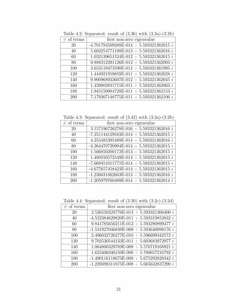
Table 4.2: Separated: result of (3.36) with (3.2a)-(3.2b)# of terms first non-zero eigenvalue
20 -4.701794509288E-014 + 5.593321362015 i
40 5.602254771198E-013 + 5.593321362016 i
60 1.032139651524E-012 + 5.593321362015 i
80 9.888312391126E-012 + 5.593321362003 i
100 3.653119473590E-012 + 5.593321361995 i
120 1.444921959859E-011 + 5.593321362028 i
140 9.900968933607E-012 + 5.593321362045 i
160 1.439803831715E-011 + 5.593321362063 i
180 1.945150984728E-011 + 5.593321362153 i
200 7.179307148775E-011 + 5.593321362106 i
Table 4.3: Separated: result of (3.42) with (3.2a)-(3.2b)# of terms first non-zero eigenvalue
20 3.157196726278E-016 + 5.593321362016 i
40 -7.251144129583E-014 + 5.593321362015 i
60 4.255485395489E-014 + 5.593321362016 i
80 -4.264470720994E-014 + 5.593321362015 i
100 1.506850200172E-013 + 5.593321362015 i
120 1.480550572549E-014 + 5.593321362015 i
140 -7.669451011771E-014 + 5.593321362015 i
160 -4.677657458423E-014 + 5.593321362015 i
180 -1.236031862663E-013 + 5.593321362016 i
200 -1.205979760499E-014 + 5.593321362014 i
Table 4.4: Separated: result of (3.30) with (3.2c)-(3.2d)# of terms first non-zero eigenvalue
20 2.526550228776E-013 + 5.593321366400 i
40 -4.522384629820E-011 + 5.593319852832 i
60 9.841785656211E-013 + 5.593280899477 i
80 -1.531927046838E-009 + 5.593640098176 i
100 2.496032726277E-010 + 5.596699342572 i
120 9.702530544133E-011 + 5.603683972977 i
140 1.064800329789E-008 + 5.570719168921 i
160 1.623406346150E-008 + 5.780657216792 i
180 -1.490116118673E-008 + 5.675292828342 i
200 -1.239398311875E-008 + 5.665632837290 i
21
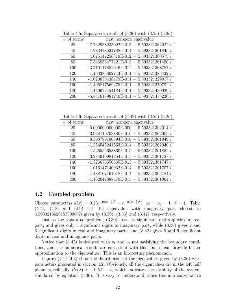
Table 4.5: Separated: result of (3.36) with (3.2c)-(3.2d)# of terms first non-zero eigenvalue
20 7.742938235022E-015 + 5.593321362022 i
40 1.283478531788E-014 + 5.593321361845 i
60 4.075147256319E-012 + 5.593321360575 i
80 7.546856477421E-013 + 5.593321361450 i
100 3.710117852046E-012 + 5.593321368787 i
120 1.153386862743E-011 + 5.593321385432 i
140 -1.020835438479E-011 + 5.593321329017 i
160 -1.406817569475E-011 + 5.593321370792 i
180 1.150672454184E-011 + 5.593321430929 i
200 -5.847618981240E-011 + 5.593321475230 i
Table 4.6: Separated: result of (3.42) with (3.2c)-(3.2d)# of terms first non-zero eigenvalue
20 0.000000000000E-000 + 5.593321362014 i
40 -3.928140703880E-016 + 5.593321362005 i
60 8.398799190894E-016 + 5.593321361949 i
80 -1.254545241563E-014 + 5.593321362040 i
100 -1.526556658860E-015 + 5.593321361852 i
120 -3.284910984254E-015 + 5.593321361727 i
140 -1.376676550535E-013 + 5.593321361747 i
160 1.016147140932E-014 + 5.593321361707 i
180 -1.488707161018E-014 + 5.593321362184 i
200 -1.162047888470E-015 + 5.593321361964 i
4.2 Coupled problem
Choose parameters k(x) = 0.1(e−16(x− 1
2)2 + e−16(x+ 1
2)2), p1 = p2 = 1, δ = 1. Table
(4.7), (4.8) and (4.9) list the eigenvalue with imaginary part closest to5.5933213620153309807i given by (3.30), (3.36) and (3.42), respectively.
Just as the separated problem, (3.30) loses its significant digits quickly in realpart, and gives only 3 significant digits in imaginary part, while (3.36) gives 2 and6 significant digits in real and imaginary parts, and (3.42) gives 5 and 9 significantdigits in real and imaginary parts.
Notice that (3.42) is deduced with v1 and v2 not satisfying the boundary condi-tions, and the numerical results are consistent with this, but it can provide betterapproximation to the eigenvalues. This is an interesting phenomenon.
Figures (4.1)-(4.3) show the distribution of the eigenvalues given by (3.36) withparameters presented in section 4.2. Obviously, all the eigenvalues are in the left halfplane, specifically Re(λ) < −0.5E − 4, which indicates the stability of the systemsimulated by equation (3.36). It is easy to understand, since this is a conservative
22
system with internal energy dissipation, so it must be stable.
Table 4.7: Coupled: result of (3.30)# of terms eigenvalue closest to 5.5933213620153309807i
20 -1.696600794218E-003 + 5.593587490912 i
40 -2.014203095153E-003 + 5.593647464088 i
60 -2.013375812398E-003 + 5.593647220497 i
80 -2.016298462637E-003 + 5.593645643022 i
100 -2.000675748912E-003 + 5.593645196102 i
120 -2.022480683191E-003 + 5.593662912802 i
140 -1.654820503910E-003 + 5.593318134435 i
160 -2.224705539659E-003 + 5.592515222158 i
180 3.560195441660E-003 + 5.582907446855 i
200 -7.681585147621E-004 + 5.591396320852 i
Table 4.8: Coupled: result of (3.36)# of terms eigenvalue closest to 5.5933213620153309807i
20 -3.074759362660E-004 + 5.593372889475 i
40 -3.654157349264E-004 + 5.593383211466 i
60 -3.652607020196E-004 + 5.593383186288 i
80 -3.652532971138E-004 + 5.593383184428 i
100 -3.652398643337E-004 + 5.593383186897 i
120 -3.653078373088E-004 + 5.593383157640 i
140 -3.652671952068E-004 + 5.593383142103 i
160 -3.654157221780E-004 + 5.593383161375 i
180 -3.651049628948E-004 + 5.593383093593 i
200 -3.651957999956E-004 + 5.593384157939 i
23
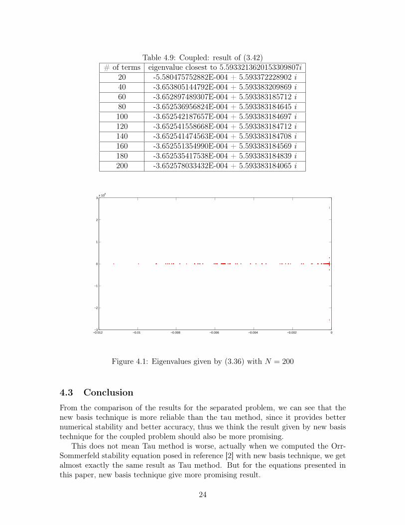
Table 4.9: Coupled: result of (3.42)# of terms eigenvalue closest to 5.5933213620153309807i
20 -5.580475752882E-004 + 5.593372228902 i
40 -3.653805144792E-004 + 5.593383209869 i
60 -3.652897489307E-004 + 5.593383185712 i
80 -3.652536956824E-004 + 5.593383184645 i
100 -3.652542187657E-004 + 5.593383184697 i
120 -3.652541558668E-004 + 5.593383184712 i
140 -3.652541474563E-004 + 5.593383184708 i
160 -3.652551354990E-004 + 5.593383184569 i
180 -3.652535417538E-004 + 5.593383184839 i
200 -3.652578033432E-004 + 5.593383184065 i
−0.012 −0.01 −0.008 −0.006 −0.004 −0.002 0−3
−2
−1
0
1
2
3x 10
8
Figure 4.1: Eigenvalues given by (3.36) with N = 200
4.3 Conclusion
From the comparison of the results for the separated problem, we can see that thenew basis technique is more reliable than the tau method, since it provides betternumerical stability and better accuracy, thus we think the result given by new basistechnique for the coupled problem should also be more promising.
This does not mean Tau method is worse, actually when we computed the Orr-Sommerfeld stability equation posed in reference [2] with new basis technique, we getalmost exactly the same result as Tau method. But for the equations presented inthis paper, new basis technique give more promising result.
24

−5.5396 −5.5394 −5.5392 −5.539 −5.5388 −5.5386 −5.5384 −5.5382
x 10−3
−3
−2
−1
0
1
2
3
x 104
Figure 4.2: Zoom-in of part of figure (4.1)
−3.5 −3 −2.5 −2 −1.5 −1 −0.5 0
x 10−4
−8
−6
−4
−2
0
2
4
6
8
x 106
Figure 4.3: Zoom-in of part of figure (4.1)
25
This paper demonstrates how to apply the new basis technique to a one-dimensionproblem, it is valuable to study whether or not it can be applied to higher dimensionproblem and how to do that.
A Appendix
Here are some properties of Chebyshev polynomials:
T0(x) = 1
T1(x) = x
Tn(x) = 2xTn−1(x) − Tn−2(x), n ≥ 2
Tn(±1) = (±1)n, n = 0, 1, . . .
dk
dxkTn(±1) = (±1)n+k
∏k−1m=0(n
2 − m2)
(2k − 1)!!, k ≥ 1, n = 0, 1, . . . (A.1)
Particularly,
d3
dx3Tn(±1) = (±1)n+3 n2(n2 − 1)(n2 − 4)
15d2
dx2Tn(±1) = (±1)n+2 n2(n2 − 1)
3d
dxTn(±1) = (±1)n+1n2
Define inner product
〈u, v〉 =
∫ 1
−1
uv√1 − x2
dx,
then
〈Ti(x), Tj(x)〉 =
π, i = j = 0π2, i = j 6= 0
0, i 6= j
Suppose
f(x) =N
∑
n=0
anTn(x),dk
dxkf(x) =
N∑
n=0
a(k)n Tn(x)
the relationship between an and a(k)n is known as recurrence rule:
cn−1a(k)n−1 = 2na(k−1)
n + a(k)n+1, n ≥ 1, k ≥ 1 (A.2)
where
cj =
{
2, j = 0
1, j = 1, 2, . . .
26
By (A.2) and mathematical induction, it can be shown that
a(k)0
a(k)1...
a(k)N
= M k
a0
a1...
aN
(A.3)
where matrix M , depending only on N , is generated from (A.2) as below.
Consider k = 1. Obviously a(1)N = 0, because the order of the polynomial is
decreased by one after taking its first derivative. Therefore the coefficient of the N th
order term must be 0.Second, a
(1)N−1 = 2NaN , because
T0(x) = 1
T1(x) = x = 21−1x
T2(x) = 2x2 − 1 = 22−1x2 + . . .
T3(x) = 4x3 + . . . = 23−1x3 + . . .
...
Tn−1(x) = 2n−2xn−1 + . . .
Tn(x) = 2n−1xn + . . .
dTn(x)
dx= n ∗ 2n−1xn−1 + . . . = 2n ∗ 2n−2xn−1 + . . .
= 2nTn−1(x) + . . .
After taking the first derivative of a polynomial of order N , it becomes a polynomialof order N − 1. From the above calculation the term of order N − 1 is TN−1(x) whichis obtained from the first derivative of aNTN(x). Therefore using the result above, we
get that a(1)N−1 = 2NaN .
Now that a(1)N = 0 and a
(1)N−1 = 2NaN , by (A.2), all the coefficients can be com-
puted one by one, from a(1)N−2, a
(1)N−3, . . ., until a
(1)0 .
Suppose a(1)n =
∑N
i=0 sn,iai, n = 0, . . . , N , then we have
a(1)0
a(1)1...
a(1)N
= M
a0
a1...
aN
where
M =
s0,0 s0,1 . . . s0,N
s1,0 s1,1 . . . s1,N
...sN,0 sN,1 . . . sN,N
27
B Matlab Code
B.1 report
Listing B.1: report.m1 % main f i l e2
3 clear ;4 close a l l ;5
6 % N i s between n1 and n27 n1 = 20 ;8 n2 = 200 ;9
10 % keep only e i g enva l u e s o f l e n g t h < rad ius wi th11 % non−nega t i v e imaginary par t12 rad iu s = 300 ;13
14 % Tau method : separa ted problem15 for p = 1 :2 %boundary cond i t i on : 1 or 216 for r = 0 :1 %damping term : 0 or 117 r e s = [ ] ;18 tmp = Tau1Beam(n1 , r , p ) ;19 tmp = tmp( imag(tmp)>=0) ;20 tmp = tmp(abs (tmp) < rad iu s ) ;21 tmp = sort (tmp) ;22 r e s ( 1 , : ) = tmp ;23 for m = n1+1:n224 tmp = Tau1Beam(m, r , p ) ;25 pL = length ( r e s (m−n1 , : ) ) ;26 for k = 1 :pL27 r e s (m−n1+1,k ) = GetClosestPoint (tmp , r e s (m−n1 , k ) ) ;28 end
29 end
30 for m = 1 :pL31 DrawSave1 (0 , r e s ( : ,m) , r , p , 0 , n1 , n2 ) ;32 end
33 end
34 end
35
36 % Tau method : coup led problem37 for r = 0 :1 %damping term : 0 or 138 r e s = [ ] ;39 tmp = Tau2Beam(n1 , r ) ;40 tmp = tmp( imag(tmp)>=0) ;41 tmp = tmp(abs (tmp) < rad iu s ) ;42 tmp = sort (tmp) ;43 r e s ( 1 , : ) = tmp ;44 for m = n1+1:n245 tmp = Tau2Beam(m, r ) ;46 pL = length ( r e s (m−n1 , : ) ) ;47 for k = 1 :pL48 r e s (m−n1+1,k ) = GetClosestPoint (tmp , r e s (m−n1 , k ) ) ;
28
49 end
50 end
51 for m = 1 :pL52 DrawSave2 (0 , r e s ( : ,m) , r , 1 , n1 , n2 ) ;53 end
54 end
55
56 % New ba s i s t ech : v1 & v2 use boundary cond i t i on : separa ted problem57 for p = 1 :2 %boundary cond i t i on : 1 or 258 for r = 0 :1 %damping term : 0 or 159 r e s = [ ] ;60 tmp = NBUseBC1Beam(n1 , r , p ) ;61 tmp = tmp( imag(tmp)>=0) ;62 tmp = tmp(abs (tmp) < rad iu s ) ;63 tmp = sort (tmp) ;64 r e s ( 1 , : ) = tmp ;65 for m = n1+1:n266 tmp = NBUseBC1Beam(m, r , p ) ;67 pL = length ( r e s (m−n1 , : ) ) ;68 for k = 1 :pL69 r e s (m−n1+1,k ) = GetClosestPoint (tmp , r e s (m−n1 , k ) ) ;70 end
71 end
72 for m = 1 :pL73 DrawSave1 (1 , r e s ( : ,m) , r , p , 0 , n1 , n2 ) ;74 end
75 end
76 end
77
78 % New ba s i s t ech : v1 & v2 use boundary cond i t i on : coup led problem79 for r = 0 :1 %damping term : 0 or 180 r e s = [ ] ;81 tmp = NBUseBC2Beam(n1 , r ) ;82 tmp = tmp( imag(tmp)>=0) ;83 tmp = tmp(abs (tmp) < rad iu s ) ;84 tmp = sort (tmp) ;85 r e s ( 1 , : ) = tmp ;86 for m = n1+1:n287 tmp = NBUseBC2Beam(m, r ) ;88 pL = length ( r e s (m−n1 , : ) ) ;89 for k = 1 :pL90 r e s (m−n1+1,k ) = GetClosestPoint (tmp , r e s (m−n1 , k ) ) ;91 end
92 end
93 for m = 1 :pL94 DrawSave2 (1 , r e s ( : ,m) , r , 1 , n1 , n2 ) ;95 end
96 end
97
98 % New ba s i s t ech : v1 & v2 no boundary cond i t i on : separa ted problem99 for p = 1 :2 %boundary cond i t i on : 1 or 2
100 for r = 0 :1 %damping term : 0 or 1101 r e s = [ ] ;102 tmp = NBNoBC1Beam(n1 , r , p ) ;
29

103 tmp = tmp( imag(tmp)>=0) ;104 tmp = tmp(abs (tmp) < rad iu s ) ;105 tmp = sort (tmp) ;106 r e s ( 1 , : ) = tmp ;107 for m = n1+1:n2108 tmp = NBNoBC1Beam(m, r , p ) ;109 pL = length ( r e s (m−n1 , : ) ) ;110 for k = 1 :pL111 r e s (m−n1+1,k ) = GetClosestPoint (tmp , r e s (m−n1 , k ) ) ;112 end
113 end
114 for m = 1 :pL115 DrawSave1 (2 , r e s ( : ,m) , r , p , 0 , n1 , n2 ) ;116 end
117 end
118 end
119
120 % New ba s i s t ech : v1 & v2 no boundary cond i t i on : coup led problem121 for r = 0 :1 %damping term : 0 or 1122 r e s = [ ] ;123 tmp = NBNoBC2Beam(n1 , r ) ;124 tmp = tmp( imag(tmp)>=0) ;125 tmp = tmp(abs (tmp) < rad iu s ) ;126 tmp = sort (tmp) ;127 r e s ( 1 , : ) = tmp ;128 for m = n1+1:n2129 tmp = NBNoBC2Beam(m, r ) ;130 pL = length ( r e s (m−n1 , : ) ) ;131 for k = 1 :pL132 r e s (m−n1+1,k ) = GetClosestPoint (tmp , r e s (m−n1 , k ) ) ;133 end
134 end
135 for m = 1 :pL136 DrawSave2 (2 , r e s ( : ,m) , r , 1 , n1 , n2 ) ;137 end
138 end
B.2 c
Listing B.2: c.m1 % c ( k )2 function r = c (k )3 i f ( k==0)4 r = 2 . 0 ;5 else
6 r = 1 . 0 ;7 end
8 end
B.3 ChebyshevExpansion
Listing B.3: ChebyshevExpansion.m1 % compute the c o e f f i c i e n t s o f the Chebyshev expans ions
30
2 % for the g iven func3 function r = ChebyshevExpansion ( func , n)4 r=zeros (1 , n+1) ;5 f 1 = func (1 ) ;6 f 2 = func (−1) ;7 t=1:n−1;8 for m=0:n9 tmp = ( f1 + f2 ) /2 ;
10 tmp = tmp + func ( cos (pi∗ t /n) ) ∗ cos (pi∗m∗ t /n) ’ ;11 i f (m==0 | | m==n)12 r (m+1) = tmp/n ;13 else
14 r (m+1) = 2∗tmp/n ;15 end
16 f 2 = −f 2 ;17 end
18 end
B.4 ChebyshevMultiplication
Listing B.4: ChebyshevMultiplication.m1 % formula f o r f ( x ) g ( x ) where f ( x ) and g ( x ) are expans ions2 % in term of Chebyshev b a s i s3 function r = ChebyshevMult ip l i cat ion ( c1 )4 L = length ( c1 )−1;5 r = zeros (2∗L+1,L+1) ;6 for n = 0 :L7 for m = 0 :L8 r (m+n+1, m+1) = r (m+n+1, m+1) + c1 (n+1) /2 ;9 i f m>=n
10 k = m − n ;11 else
12 k = n − m;13 end
14 r ( k+1, m+1) = r (k+1, m+1) + c1 (n+1) /2 ;15 end
16 end
17 end
B.5 GetClosestPoint
Listing B.5: GetClosestPoint.m1 % choose a complex number from ptmp which i s c l o s e s t to apo in t2 function r = GetClosestPoint (ptmp , apoint )3 t = 0 . 0 1 ;4 l = 0 ;5 while l <16 t = t ∗ 2 ;7 tmp1 = ptmp(abs (ptmp − apoint )<=t ) ;8 l = length ( tmp1) ;9 end
10 best = 1 ;
31
11 i f l ~= 112 bestD = 1E20 ;13 for t = 1 : l14 curD = abs ( tmp1( t ) − apoint ) ;15 i f curD < bestD16 best = t ;17 bestD = curD ;18 end
19 end
20 end
21 r = tmp1( best ) ;22 end
B.6 DrawSave1
Listing B.6: DrawSave1.m1 % p l o t the numerical r e s u l t f o r separa ted problem , then save the2 % p l o t in t o . pdf f i l e s , and save the numerical r e s u l t i n t o . t x t3 % f i l e s4 function r = DrawSave1 (nTech , data , damp , nBCond , nMeth , nTerm1 ,
nTerm2)5 sTech = { ’Tau ’ ; ’NB−UseBC ’ ; ’NB−NoBC ’ } ;6 sMeth = { ’OneBeam ’ ; ’TwoBeams ’ } ;7 sDamp = { ’ damping=0 ’ ; ’ damping=1 ’ } ;8 sBC = { ’ 1 st_derivative_BC ’ ; ’ 2nd&3rd_derivative_BC ’ } ;9
10 r = f igure (1 ) ;11 orient l andscape ;12 subplot ( 2 , 1 , 1 ) ;13 plot (nTerm1 : nTerm2 , imag( data ) , ’ . r ’ ) ;14 ylabel ( ’ imaginary ’ ) ;15 i f (nBCond == 1)16 bcStr = ’ , ␣␣1^{ s t }␣B.C. , ␣␣ ’ ;17 e l s e i f nBCond == 218 bcStr = ’ , ␣␣2^{nd}␣B.C. , ␣␣ ’ ;19 else
20 bcStr = ’ ’ ;21 end
22 t i t l e ( [ char ( sTech ( nTech+1) ) , ’ , ␣ ’ , char ( sMeth (nMeth+1) ) , ’ , ␣ ’ ,. . .
23 ’ \ d e l t a ␣=␣ ’ , num2str(damp) , bcStr , . . .24 10 , num2str( data (1 ) , 20) ] ) ;25
26 subplot ( 2 , 1 , 2 ) ;27 plot (nTerm1 : nTerm2 , real ( data ) , ’ . r ’ ) ;28 xlabel ( ’ terms ’ ) ;29 ylabel ( ’ r e a l ’ ) ;30
31 dname = s t r c a t ( sTech ( nTech+1) , . . .32 ’ \ ’ , sMeth (nMeth+1) , . . .33 ’ \ ’ , sDamp(damp+1) , . . .34 ’ \ ’ , sDamp(damp+1) , . . .35 ’− ’ , sBC(nBCond) ) ;
32
36 i f (~ i s d i r ( char (dname) ) )37 mkdir ( char (dname) ) ;38 end
39 tmp0 = char ( s t r c a t (dname , ’ \ ’ , num2str( data (1 ) ) ) ) ;40 tmp1 = s t r c a t ( tmp0 , ’ . pdf ’ ) ;41 tmpRnd = ’ ’ ;42 while exist ( tmp1 , ’ f i l e ’ )~=043 tmpRnd = num2str( randi (10000) ) ;44 tmp1 = s t r c a t ( tmp0 , ’− ’ , tmpRnd , ’ . pdf ’ ) ;45 end
46 fname = tmp1 ;47 saveas ( r , fname , ’ pdf ’ ) ;48
49 i f isempty (tmpRnd)50 dfname = char ( s t r c a t ( tmp0 , ’ . txt ’ ) ) ;51 else
52 dfname = char ( s t r c a t ( tmp0 , ’− ’ , tmpRnd , ’ . txt ’ ) ) ;53 end
54 f i d = fopen ( dfname , ’w ’ ) ;55 fpr intf ( f i d , ’#terms\ t \ t \ t r e a l \ t \ t \ t \ t imaginary \n ’ ) ;56 for m=1: length ( data )57 fpr intf ( f i d , ’%u\ t%4.12E\ t%4.12E\n ’ , nTerm1+m−1, real ( data (m
) ) , imag( data (m) ) ) ;58 end
59 fc lose ( f i d ) ;60 end
B.7 DrawSave2
Listing B.7: DrawSave2.m1 % p l o t the numerical r e s u l t f o r coup led problem , then save the2 % p l o t in t o . pdf f i l e s , and save the numerical r e s u l t i n t o . t x t3 % f i l e s4 function r = DrawSave2 (nTech , data , damp , nMeth , nTerm1 , nTerm2)5 sTech = { ’Tau ’ ; ’NB−UseBC ’ ; ’NB−NoBC ’ } ;6 sMeth = { ’OneBeam ’ ; ’TwoBeams ’ } ;7 sDamp = { ’ damping=0 ’ ; ’ damping=1 ’ } ;8
9 r = f igure (1 ) ;10 orient l andscape ;11 subplot ( 2 , 1 , 1 ) ;12 plot (nTerm1 : nTerm2 , imag( data ) , ’ . r ’ ) ;13 ylabel ( ’ imaginary ’ ) ;14 t i t l e ( [ char ( sTech ( nTech+1) ) , ’ , ␣ ’ , char ( sMeth (nMeth+1) ) , ’ , ␣ ’ ,
. . .15 ’ \ d e l t a ␣=␣ ’ , num2str(damp) , . . .16 10 , num2str( data (1 ) , 20) ] ) ;17
18 subplot ( 2 , 1 , 2 ) ;19 plot (nTerm1 : nTerm2 , real ( data ) , ’ . r ’ ) ;20 xlabel ( ’ terms ’ ) ;21 ylabel ( ’ r e a l ’ ) ;22
33
23 dname = s t r c a t ( sTech ( nTech+1) , . . .24 ’ \ ’ , sMeth (nMeth+1) , . . .25 ’ \ ’ , sDamp(damp+1) ) ;26 i f (~ i s d i r ( char (dname) ) )27 mkdir ( char (dname) ) ;28 end
29 tmp0 = char ( s t r c a t (dname , ’ \ ’ , num2str( data (1 ) ) ) ) ;30 tmp1 = s t r c a t ( tmp0 , ’ . pdf ’ ) ;31 tmpRnd = ’ ’ ;32 while exist ( tmp1 , ’ f i l e ’ )~=033 tmpRnd = num2str( randi (10000) ) ;34 tmp1 = s t r c a t ( tmp0 , ’− ’ , tmpRnd , ’ . pdf ’ ) ;35 end
36 fname = tmp1 ;37 saveas ( r , fname , ’ pdf ’ ) ;38
39 i f isempty (tmpRnd)40 dfname = char ( s t r c a t ( tmp0 , ’ . txt ’ ) ) ;41 else
42 dfname = char ( s t r c a t ( tmp0 , ’− ’ , tmpRnd , ’ . txt ’ ) ) ;43 end
44 f i d = fopen ( dfname , ’w ’ ) ;45 fpr intf ( f i d , ’#terms\ t \ t \ t r e a l \ t \ t \ t \ t imaginary \n ’ ) ;46 for m=1: length ( data )47 fpr intf ( f i d , ’%u\ t%4.12E\ t%4.12E\n ’ , nTerm1+m−1, real ( data (m
) ) , imag( data (m) ) ) ;48 end
49 fc lose ( f i d ) ;50 end
B.8 Tau1Beam
Listing B.8: Tau1Beam.m1 % tau method f o r separa ted problem2 function r = Tau1Beam(nTerms , damp , nBCond)3 N0 = nTerms ;4 Nb = 4 ;5 N = N0 + Nb;6
7 p = 1 ;8 de l t a = damp ;9
10 kcu = zeros (N0+1,N+1) ;11
12 DM = zeros (N+1,N+1) ;13 DM(N,N+1) = 2∗N/c (N−1) ;14 for m=N−2:−1:015 DM(m+1,m+2) = DM(m+1,m+2) + 2∗(m+1) ;16 DM(m+1 , :) = (DM(m+1 , :) + DM(m+3 , :) ) / c (m) ;17 end
18 DM2 = DM^2;19 DM3 = DM2 ∗ DM;20 DM4 = DM3 ∗ DM;
34
21
22 tmpOnes = ones (1 ,N+1) ;23 tmpAltOnes = (−1) . ^ ( 0 :N) ;24
25 W1 = [ tmpAltOnes ; . . .26 tmpOnes ; . . .27 tmpAltOnes ∗ DM; . . .28 sum(DM) ] ;29
30 W2 = [ tmpAltOnes ∗ DM2; . . .31 sum(DM2) ; . . .32 tmpAltOnes ∗ DM3; . . .33 sum(DM3) ] ;34
35 BC1 = −W1( : , N−2:N+1) \ W1( : , 1 :N−3) ;36 BC2 = −W2( : , N−2:N+1) \ W2( : , 1 :N−3) ;37 V1 = [ eye (N0+1) ; BC1 ] ;38 V2 = [ eye (N0+1) ; BC2 ] ;39
40 DM4p = DM4( 1 :N0+1 , :) ;41 i f nBCond == 242 A=[zeros (N0+1) , eye (N0+1) ; . . .43 (−p∗DM4p−kcu ) ∗V2 , −de l t a ∗kcu∗V2 ] ;44 else
45 A=[zeros (N0+1) , eye (N0+1) ; . . .46 (−p∗DM4p−kcu ) ∗V1 , −de l t a ∗kcu∗V1 ] ;47 end
48 t = A;49 [V,D] = eig ( t ) ;50 r = diag (D) ;51
52 end
B.9 Tau2Beam
Listing B.9: Tau2Beam.m1 % tau method f o r coup led problem2 function [ r , c r ] = Tau2Beam(nTerms , damp)3 N0 = nTerms ;4 Nb = 4 ;5 N = N0 + Nb;6
7 p1 = 1 ;8 p2 = 1 ;9 de l t a = damp ;
10
11 ct = 1/2 ;12 sigma = 1/16 ;13 func = @(x )exp(−((x−ct ) / sigma ) .^2) + exp(−((x+ct ) / sigma ) .^2) / 1 0 . 0 ;14
15 kc = ChebyshevExpansion ( func , N) ;16 kcu = ChebyshevMult ip l i cat ion ( kc ) ;17 kcu = kcu ( 1 :N0+1 , :) ;
35
18
19 DM = zeros (N+1,N+1) ;20 DM(N,N+1) = 2∗N/c (N−1) ;21 for m=N−2:−1:022 DM(m+1,m+2) = DM(m+1,m+2) + 2∗(m+1) ;23 DM(m+1 , :) = (DM(m+1 , :) + DM(m+3 , :) ) / c (m) ;24 end
25 DM2 = DM^2;26 DM3 = DM2 ∗ DM;27 DM4 = DM3 ∗ DM;28
29 tmpOnes = ones (1 ,N+1) ;30 tmpAltOnes = (−1) . ^ ( 0 :N) ;31
32 W1 = [ tmpAltOnes ; . . .33 tmpOnes ; . . .34 tmpAltOnes ∗ DM; . . .35 sum(DM) ] ;36
37 W2 = [ tmpAltOnes ∗ DM2; . . .38 sum(DM2) ; . . .39 tmpAltOnes ∗ DM3; . . .40 sum(DM3) ] ;41
42 BC1 = −W1( : , N−2:N+1) \ W1( : , 1 :N−3) ;43 BC2 = −W2( : , N−2:N+1) \ W2( : , 1 :N−3) ;44 V1 = [ eye (N0+1) ; BC1 ] ;45 V2 = [ eye (N0+1) ; BC2 ] ;46
47 DM4p = DM4( 1 :N0+1 , :) ;48 A=[zeros (N0+1) , zeros (N0+1) , eye (N0+1) , zeros (N0+1) ;
. . .49 zeros (N0+1) , zeros (N0+1) , zeros (N0+1) , eye (N0+1) ;
. . .50 (−p1∗DM4p−kcu ) ∗V1 , kcu∗V2 , −de l t a ∗kcu∗V1 , zeros (N0+1) ;
. . .51 kcu∗V1 , (−p2∗DM4p−kcu ) ∗V2 , zeros (N0+1) , −de l t a ∗kcu∗V2
] ;52
53 [V,D] = eig (A) ;54 r = diag (D) ;55
56 end
B.10 NBUseBC1Beam
Listing B.10: NBUseBC1Beam.m1 % new ba s i s t ech wi th v1 & v2 s a t i s f y i n g boundary cond i t i on s2 % for separa ted problem3 function [ r , v ] = NBUseBC1Beam(nTerms , damp , nBCond)4 N0 = nTerms ;5 Nb = 4 ;6 N = N0 + Nb;
36
7
8 p1 = 1 ;9 p2 = 1 ;
10 de l t a = damp ;11
12 ct = 1/2 ;13 sigma = 1/16 ;14 func = @(x ) (exp(−((x−ct ) / sigma ) .^2) + exp(−((x+ct ) / sigma ) .^2) ) / 1 0 . 0 ;15
16 K = zeros (N+1) ;17
18 DM = zeros (N+1) ;19 DM(N,N+1) = 2.0∗N/c (N−1) ;20 for m=N−2:−1:021 DM(m+1,m+2) = DM(m+1,m+2) + 2 . 0∗ (m+1) ;22 DM(m+1 , :) = (DM(m+1 , :) + DM(m+3 , :) ) / c (m) ;23 end
24 DM4 = DM ^ 4 ;25
26 B1 = zeros (N0+5,N0+1) ;27 B2 = zeros (N0+5,N0+1) ;28 for m=1:N0+129 B1(m,m) = 1 . 0 ;30 B1(m+2,m) = −2.0∗(m+1)/(m+2.0) ;31 B1(m+4,m) = m/(m+2.0) ;32
33 B2(m,m) = 1 . 0 ;34 B2(m+2,m) = −2.0∗(m−2)∗(m−1)^2/((m+1.0) ∗(m+2.0) ^2) ;35 B2(m+4,m) = (m−2)∗(m−1)^2∗m^2/((m+4)∗(6 .0+5.0∗m+m^2)^2) ;36 end
37
38 B1p = B1 ( 1 :N0+1 , :) ;39 B2p = B2 ( 1 :N0+1 , :) ;40 C1 = −(p1∗DM4+K) ∗B2 ;41 C1 = C1 ( 1 :N0+1 , :) ;42 C2 = −(p2∗DM4+K) ∗B1 ;43 C2 = C2 ( 1 :N0+1 , :) ;44 D1 = K∗B2 ;45 D1 = D1( 1 :N0+1 , :) ;46 D2 = K∗B1 ;47 D2 = D2( 1 :N0+1 , :) ;48
49 i f nBCond == 250 eigA = [ zeros (N0+1) , eye (N0+1) ; . . .51 C1 , −de l t a ∗D1 ] ;52 eigB = [ eye (N0+1) , zeros (N0+1) ; . . .53 zeros (N0+1) , B2p ] ;54 else
55 eigA = [ zeros (N0+1) , eye (N0+1) ; . . .56 C2 , −de l t a ∗D2 ] ;57 eigB = [ eye (N0+1) , zeros (N0+1) ; . . .58 zeros (N0+1) , B1p ] ;59 end
60 t = eigB\eigA ;
37

61 [ v ,D] = eig ( t ) ;62 r = diag (D) ;63
64
65 end
B.11 NBUseBC2Beam
Listing B.11: NBUseBC2Beam.m1 % new ba s i s t ech wi th v1 & v2 s a t i s f y i n g boundary cond i t i on s2 % for coup led problem3 function [ r , c r ] = NBUseBC2Beam(nTerms , damp)4 N0 = nTerms ;5 Nb = 4 ;6 N = N0 + Nb;7
8 p1 = 1 ;9 p2 = 1 ;
10 de l t a = damp ;11
12 ct = 1/2 ;13 sigma = 1/16 ;14 func = @(x ) (exp(−((x−ct ) / sigma ) .^2) + exp(−((x+ct ) / sigma ) .^2) ) / 1 0 . 0 ;15
16 K = ChebyshevMult ip l i cat ion ( ChebyshevExpansion ( func , N) ) ;17 K = K(1 :N+1 , :) ;18
19 DM = zeros (N+1) ;20 DM(N,N+1) = 2.0∗N/c (N−1) ;21 for m=N−2:−1:022 DM(m+1,m+2) = DM(m+1,m+2) + 2 . 0∗ (m+1) ;23 DM(m+1 , :) = (DM(m+1 , :) + DM(m+3 , :) ) / c (m) ;24 end
25 DM4 = DM ^ 4 ;26
27 B1 = zeros (N0+5,N0+1) ;28 B2 = zeros (N0+5,N0+1) ;29 for m=1:N0+130 B1(m,m) = 1 . 0 ;31 B1(m+2,m) = −2.0∗(m+1)/(m+2.0) ;32 B1(m+4,m) = m/(m+2.0) ;33
34 B2(m,m) = 1 . 0 ;35 B2(m+2,m) = −2.0∗(m−2)∗(m−1)^2/((m+1.0) ∗(m+2.0) ^2) ;36 B2(m+4,m) = (m−2)∗(m−1)^2∗m^2/((m+4)∗(6 .0+5.0∗m+m^2)^2) ;37 end
38 B1p = B1 ( 1 :N0+1 , :) ;39 B2p = B2 ( 1 :N0+1 , :) ;40 C1 = −(p1∗DM4+K) ∗B2 ;41 C1 = C1 ( 1 :N0+1 , :) ;42 C2 = −(p2∗DM4+K) ∗B1 ;43 C2 = C2 ( 1 :N0+1 , :) ;44 D1 = K∗B2 ;
38

45 D1 = D1( 1 :N0+1 , :) ;46 D2 = K∗B1 ;47 D2 = D2( 1 :N0+1 , :) ;48 eigA = [ zeros (N0+1) , zeros (N0+1) , eye (N0+1) , zeros (N0+1) ; . . .49 zeros (N0+1) , zeros (N0+1) , zeros (N0+1) , eye (N0+1) ; . . .50 C1 , D2 , −de l t a ∗D1, zeros (N0+1) ; . . .51 D1, C2 , zeros (N0+1) , −de l t a ∗D2 ] ;52 eigB = [ eye (N0+1) , zeros (N0+1) , zeros (N0+1) , zeros (N0+1) ; . . .53 zeros (N0+1) , eye (N0+1) , zeros (N0+1) , zeros (N0+1) ; . . .54 zeros (N0+1) , zeros (N0+1) , B2p , zeros (N0+1) ; . . .55 zeros (N0+1) , zeros (N0+1) , zeros (N0+1) , B1p ] ;56 t = eigB\eigA ;57 [V,D] = eig ( t ) ;58 r = diag (D) ;59 cr = cond( t ) ;60
61 end
B.12 NBNoBC1Beam
Listing B.12: NBNoBC1Beam.m1 % new ba s i s t ech wi th v1 & v2 not s a t i s f y i n g boundary cond i t i on s2 % for separa ted problem3 function [ r , v ] = NBNoBC1Beam(nTerms , damp , nBCond)4 N0 = nTerms ;5 Nb = 4 ;6 N = N0 + Nb;7
8 p1 = 1 ;9 p2 = 1 ;
10 de l t a = damp ;11
12 K1 = zeros (N+1) ;13 K2 = zeros (N0+1) ;14
15 DM = zeros (N+1) ;16 DM(N,N+1) = 2.0∗N/c (N−1) ;17 for m=N−2:−1:018 DM(m+1,m+2) = DM(m+1,m+2) + 2 . 0∗ (m+1) ;19 DM(m+1 , :) = (DM(m+1 , :) + DM(m+3 , :) ) / c (m) ;20 end
21 DM4 = DM ^ 4 ;22
23 B1 = zeros (N0+5,N0+1) ;24 B2 = zeros (N0+5,N0+1) ;25 for m=1:N0+126 B1(m,m) = 1 . 0 ;27 B1(m+2,m) = −2.0∗(m+1)/(m+2.0) ;28 B1(m+4,m) = m/(m+2.0) ;29
30 B2(m,m) = 1 . 0 ;31 B2(m+2,m) = −2.0∗(m−2)∗(m−1)^2/((m+1.0) ∗(m+2.0) ^2) ;32 B2(m+4,m) = (m−2)∗(m−1)^2∗m^2/((m+4)∗(6 .0+5.0∗m+m^2)^2) ;
39
33 end
34
35 B1p = B1 ( 1 :N0+1 , :) ;36 B2p = B2 ( 1 :N0+1 , :) ;37 C1 = −(p1∗DM4+K1) ∗B2 ;38 C1 = C1 ( 1 :N0+1 , :) ;39 C2 = −(p2∗DM4+K1) ∗B1 ;40 C2 = C2 ( 1 :N0+1 , :) ;41
42 i f nBCond == 243 eigA = [ zeros (N0+1) , eye (N0+1) ; . . .44 C1 , −de l t a ∗K2 ] ;45 eigB = [B2p , zeros (N0+1) ; . . .46 zeros (N0+1) , eye (N0+1) ] ;47 else
48 eigA = [ zeros (N0+1) , eye (N0+1) ; . . .49 C2 , −de l t a ∗K2 ] ;50 eigB = [B1p , zeros (N0+1) ; . . .51 zeros (N0+1) , eye (N0+1) ] ;52 end
53 t = eigB\eigA ;54 [ v ,D] = eig ( t ) ;55 r = diag (D) ;56
57 end
B.13 NBNoBC2Beam
Listing B.13: NBNoBC2Beam.m1 % new ba s i s t ech wi th v1 & v2 not s a t i s f y i n g boundary cond i t i on s2 % for coup led problem3 function [ r , c r ] = NBNoBC2Beam(nTerms , damp)4 N0 = nTerms ;5 Nb = 4 ;6 N = N0 + Nb;7
8 p1 = 1 ;9 p2 = 1 ;
10 de l t a = damp ;11
12 ct = 1/2 ;13 sigma = 1/16 ;14 func = @(x ) (exp(−((x−ct ) / sigma ) .^2) + exp(−((x+ct ) / sigma ) .^2) ) / 1 0 . 0 ;15
16 K1 = ChebyshevMult ip l i cat ion ( ChebyshevExpansion ( func , N) ) ;17 K1 = K1( 1 :N+1 , :) ;18 K2 = ChebyshevMult ip l i cat ion ( ChebyshevExpansion ( func , N0) ) ;19 K2 = K2( 1 :N0+1 , :) ;20
21 DM = zeros (N+1) ;22 DM(N,N+1) = 2.0∗N/c (N−1) ;23 for m=N−2:−1:024 DM(m+1,m+2) = DM(m+1,m+2) + 2 . 0∗ (m+1) ;
40

25 DM(m+1 , :) = (DM(m+1 , :) + DM(m+3 , :) ) / c (m) ;26 end
27 DM4 = DM ^ 4 ;28
29 B1 = zeros (N0+5,N0+1) ;30 B2 = zeros (N0+5,N0+1) ;31 for m=1:N0+132 B1(m,m) = 1 . 0 ;33 B1(m+2,m) = −2.0∗(m+1)/(m+2.0) ;34 B1(m+4,m) = m/(m+2.0) ;35
36 B2(m,m) = 1 . 0 ;37 B2(m+2,m) = −2.0∗(m−2)∗(m−1)^2/((m+1.0) ∗(m+2.0) ^2) ;38 B2(m+4,m) = (m−2)∗(m−1)^2∗m^2/((m+4)∗(6 .0+5.0∗m+m^2)^2) ;39 end
40 B1p = B1 ( 1 :N0+1 , :) ;41 B2p = B2 ( 1 :N0+1 , :) ;42 C1 = −(p1∗DM4+K1) ∗B2 ;43 C1 = C1 ( 1 :N0+1 , :) ;44 C2 = −(p2∗DM4+K1) ∗B1 ;45 C2 = C2 ( 1 :N0+1 , :) ;46 D1 = K1∗B2 ;47 D1 = D1( 1 :N0+1 , :) ;48 D2 = K1∗B1 ;49 D2 = D2( 1 :N0+1 , :) ;50 eigA = [ zeros (N0+1) , zeros (N0+1) , eye (N0+1) , zeros (N0+1) ; . . .51 zeros (N0+1) , zeros (N0+1) , zeros (N0+1) , eye (N0+1) ; . . .52 C1 , D2 , −de l t a ∗K2, zeros (N0+1) ; . . .53 D1, C2 , zeros (N0+1) , −de l t a ∗K2 ] ;54 eigB = [B2p , zeros (N0+1) , zeros (N0+1) , zeros (N0+1) ; . . .55 zeros (N0+1) , B1p , zeros (N0+1) , zeros (N0+1) ; . . .56 zeros (N0+1) , zeros (N0+1) , eye (N0+1) , zeros (N0+1) ; . . .57 zeros (N0+1) , zeros (N0+1) , zeros (N0+1) , eye (N0+1) ] ;58 t = eigB\eigA ;59 [V,D] = eig ( t ) ;60 r = diag (D) ;61 cr = 1 ;62
63 end
References
[1] David R. Gardner, Steven A. Trogdon, Rod W. Douglas, A Modified Tau Spectral
Method That Eliminates Spurious Eigenvalues, Journal of Computational Physics,Vol. 80, No. 1, January 1989
[2] Steven A. Orszag, Accurate Solution of the Orr-Sommerfeld Stability Equation,Journal of Fluid Mechanics(1971), Vol. 50, part 4, pp 689
[3] C. Canuto, M. Y. Hussaini, A. Quarteroni, T. A. Zang, Spectral Methods: Funda-
mentals in Single Domains, Springer Press, 2006
41


![GENERALIZED CHEBYSHEV POLYNOMIALS AND POSITIVITY … › ... › rr80.pdf · Chebyshev polynomials continuing the investigation initiated in [Dup09a, Dup09d]. Cluster algebras were](https://img.pdfslide.us/doc/110x75/5f1588677af4bc0c9c1c6f20/generalized-chebyshev-polynomials-and-positivity-a-a-rr80pdf-chebyshev.jpg)