Embed Size (px)
Citation preview
1
A simple approach to q- Chebyshev polynomials
Johann Cigler
Fakultät für Mathematik, Universität Wien
Abstract
It is shown that some q analogues of the Fibonacci and Lucas polynomials lead to q analogues of the Chebyshev polynomials which retain most of their elementary properties.
1. Introduction
Let me first sketch the context from which this paper originated. I have been interested in q analogues of bivariate Fibonacci and Lucas polynomials with simple formulae as well as simple recurrences. The Fibonacci polynomials admit many such analogues but for the Lucas polynomials the situation is more complicated (see e.g. [5]). It turned out that by introducing an additional parameter both aims can be accomplished. A special choice of this parameter led me to a q analogue of the bivariate Chebyshev polynomials which admits simple generalizations of
many properties of the classical univariate Chebyshev polynomials. Some variants of these polynomials (i.e. the Al-Salam and Ismail polynomials) previously occurred in [1] and have been studied in [6] from another point of view.
To make the paper intelligible for non-specialists let me first recall some well-known facts about these polynomials.
The Fibonacci polynomials ( , )nF x s are defined by the recursion
1 2( , ) ( , ) ( , )n n nF x s xF x s sF x s (1.1)
with initial values 0( , ) 0F x s and 1( , ) 1.F x s They have the explicit expression
1
21 2
0
1( , ) .
n
k n kn
k
n kF x s s x
k
(1.2)
The Lucas polynomials ( , )nL x s satisfy the same recursion
1 2( , ) ( , ) ( , )n n nL x s xL x s sL x s (1.3)
2
with initial values 0( , ) 2L x s and 1( , ) .L x s x They are given by
2
2
0
( , ) .
n
k n kn
k
n knL x s s x
kn k
(1.4)
These polynomials satisfy a multitude of identities most of which can be proved by using Binet’s formulae
( , )n n
nF x s
(1.5)
and
( , ) n nnL x s (1.6)
where 2 4
2
x x s and
2 4
2
x x s are the roots of the equation 2 .z xz s
Unfortunately there are no simple q analogues of Binet’s formulae. Useful substitutes are the Fibonacci matrices
1
1
( , ) ( , )
( , ) ( , )n nn
n n
sF x s F x sC
sF x s F x s
(1.7)
where 0 1
Cs x
satisfies the equation 2 .C xC sI
Here 1 0
0 1I
is the 2 2x identity matrix.
The Lucas polynomial ( , )nL x s coincides with the trace
1 1( , ) ( , ) ( , )nn n nL x s tr C F x s sF x s (1.8)
of the Fibonacci matrix .nC The reader is referred to [5] for details. As is well known a sequence np of monic polynomials of degree deg np n is orthogonal with
respect to some linear functional , i.e. 0n mp p for n m and 2 0np , if and only if
it satisfies a three-term recurrence of the form 1 2( ) ( ) ( ) ( ).n n n n np x x s p x t p x This functional
3
is uniquely determined by [ 0].np n (Here we use Iverson’s convention: If a property p
is true then [ ] 1,p otherwise [ ] 0.p ) The numbers nx are called the associated moments.
The Fibonacci and Lucas polynomials satisfy the 3-term recurrence (1.1) and are therefore orthogonal.
The bivariate Chebyshev polynomials ( , )nT x s of the first kind can be defined by the recursion
1 2( , ) 2 ( , ) ( , )n n nT x s xT x s sT x s (1.9)
with initial values 0 ( , ) 1T x s and 1( , ) .T x s x
The classical Chebyshev polynomials ( ) ( , 1)n nT x T x are characterized by the identity
cos (cos ).nn T (1.10)
The polynomials ( , )nT x s are related to the Lucas polynomials by
1 2 21( , ) 2 , .
4 2
n nn
n n
sT x s L x x x s x x s
(1.11)
The bivariate Chebyshev polynomials ( , )nU x s of the second kind can be defined by the same
recursion
1 2( , ) 2 ( , ) ( , )n n nU x s xU x s sU x s (1.12)
with initial values 0 ( , ) 1U x s and 1( , ) 2 .U x s x
The classical polynomials ( ) ( , 1)n nU x U x are characterized by the identity
sin ( 1)
(cos ).sin n
nU
(1.13)
4
The bivariate polynomials of the second kind are related to the Fibonacci polynomials by
1 1
2 2
1 2( , ) 2 , .
4 2
n n
nn n
x x s x x ssU x s F x
x s
(1.14)
Both types of Chebyshev polynomials are characterized by the identity
2 21( , ) ( , )
n
n nx x s T x s U x s x s (1.15)
if we set 1( , ) 0.U x s
The classical Chebyshev polynomials are solutions of the following eigenvalue problems:
2 2( 1) ( ) ( ) ( )n n nx T x xT x n T x (1.16)
and
2( 1) ( ) 3 ( ) ( 2) ( ).n n nx U x xU x n n U x (1.17)
They also satisfy the Rodrigues-type formulae
1
2 2 2( 1)( ) 1 (1 )
(2 1)!!
nnn
n
dT x x x
n dx
(1.18)
and
1
2 2
2
( 1) ( 1) 1( ) (1 ) .
(2 1)!! 1
nn n
n
n dU x x
n dxx
(1.19)
Here we use the symbol 0
(2 1)!! (2 1).n
j
n j
More information and references about the classical Chebyshev polynomials can be found in [7], Section 9.8.2.
5
2. (q,b) - Fibonacci polynomials
We employ the usual abbreviations of q analysis such as the q Pochhammer symbols
1; (1 )(1 ) (1 ),n
na q a qa q a
0
; (1 )j
j
a q q a
and
; 1; .
; ;n nn
n
a qa q
q a q q a q
The q binomial coefficients are denoted by
;.
; ;n
q k n k
q qn n
k k q q q q
In place of
1
n
we write [ ].n
We will also need the q binomial theorem in the form
0
; ( ; ).
; ( ; )kk
k k
a q az qz
q q z q
(2.1)
As is well known (cf. e.g. [2] or [5]) the Carlitz q Fibonacci polynomials
2
1
21 2
0
1( , , )
n
k k n kn
k
n kF x s q q s x
k
(2.2)
satisfy the recursion
21 2( , , ) ( , , ) ( , , )n n nF x s q xF x qs q qsF x q s q (2.3)
with initial values 0( , , ) 0F x s q and 1( , , ) 1.F x s q
Our first aim is the study of the following q analogue of 2
, .(1 )n
sF x
b
Definition 2.1
The polynomials
2
1
21 2
0
(1 1
;, , , )
;
n
k k n k
n kk
n
k k
F x b sn k
q s xk qb q q b q
q
(2.4)
will be called ( , )q b Fibonacci polynomials.
These are polynomials in x and s whose coefficients are rational functions in .b It is clear that
for 0b they reduce to ( ,0, , ) ( , , )n nF x s q F x s q .
6
Remark
These polynomials seem to be remarkable since variants of them have occurred in the literature in
different contexts. They are closely related to the Al-Salam and Ismail polynomials ( ; , )nu x a b
which originated in [1] and are defined by the recurrence
1 21 2( ; , ) (1 ) ( ; , ) ( ; , )n n
n n nu x a b x q a u x a b q bu x a b (2.5)
with initial values 0( ; , ) 1u x a b and 1( ; , ) (1 ) .u x a b a x
It turns out that
1
( ; , )( , , , ) .
;n
n
n
u x qb qsF x b s q
qb q
(2.6)
Some properties of these polynomials have been studied in [6]. The special case b s occurred in [2]. M. Schlosser (personal communication) has observed that these polynomials can also be obtained from a specialization of his elliptic binomial Theorem (cf. [8]).
As observed in [1] we have
Theorem 2.1
The ( , )q b Fibonacci polynomials satisfy the recursion
2
1 22 1( , , , ) ( , , , ) ( , , , )
(1 )(1 )
n
n n nn n
q sF x b s q xF x b s q F x b s q
q b q b
(2.7)
with initial values 0( , , , ) 0F x b s q and 1( , , , ) 1.F x b s q
A closely related recursion gives
Theorem 2.2
The polynomials ( , , , )nF x b s q also satisfy the recursion
2 21 22
( , , , ) ( , , , ) ( , , , )(1 )(1 )n n n
qsF x b s q xF x qb qs q F x q b q s q
qb q b
(2.8)
with initial values 0( , , , ) 0F x b s q and 1( , , , ) 1.F x b s q
Both theorems can be easily verified by comparing coefficients in (2.4).
7
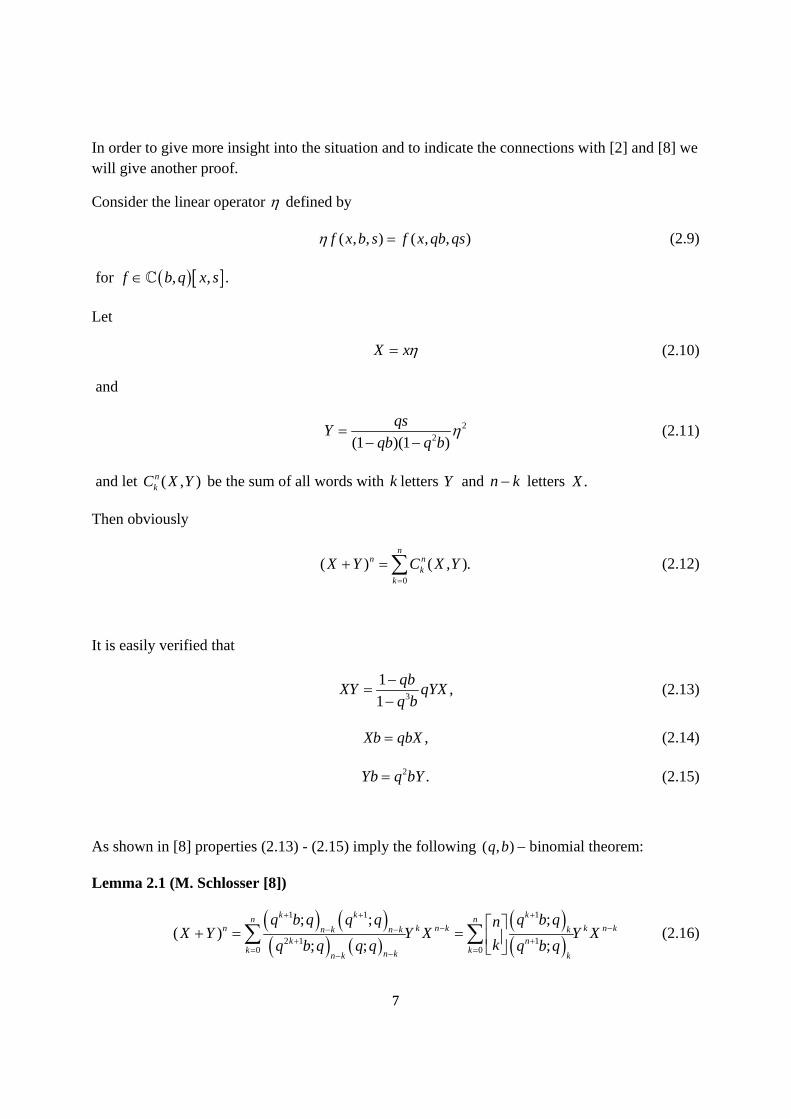
In order to give more insight into the situation and to indicate the connections with [2] and [8] we will give another proof.
Consider the linear operator defined by
( , , ) ( , , )f x b s f x qb qs (2.9)
for , , .f b q x s
Let
X x (2.10)
and
22(1 )(1 )
qs
qb q bY
(2.11)
and let ( , )nkC X Y be the sum of all words with k letters Y and n k letters .X
Then obviously
0
( ) ( , ).n
n nk
k
X Y C X Y
(2.12)
It is easily verified that
3
1,
1
qbXY qYX
q b
(2.13)
,Xb qbX (2.14)
2 .Yb q bY (2.15)
As shown in [8] properties (2.13) - (2.15) imply the following ( , )q b binomial theorem:
Lemma 2.1 (M. Schlosser [8])
1 1 1
2 1 10 0
; ; ;( )
; ; ;
k k kn nn k n k k n kn k n k k
k nk kn kn k k
q b q q q q b qnX Y Y X Y X
kq b q q q q b q
(2.16)
8
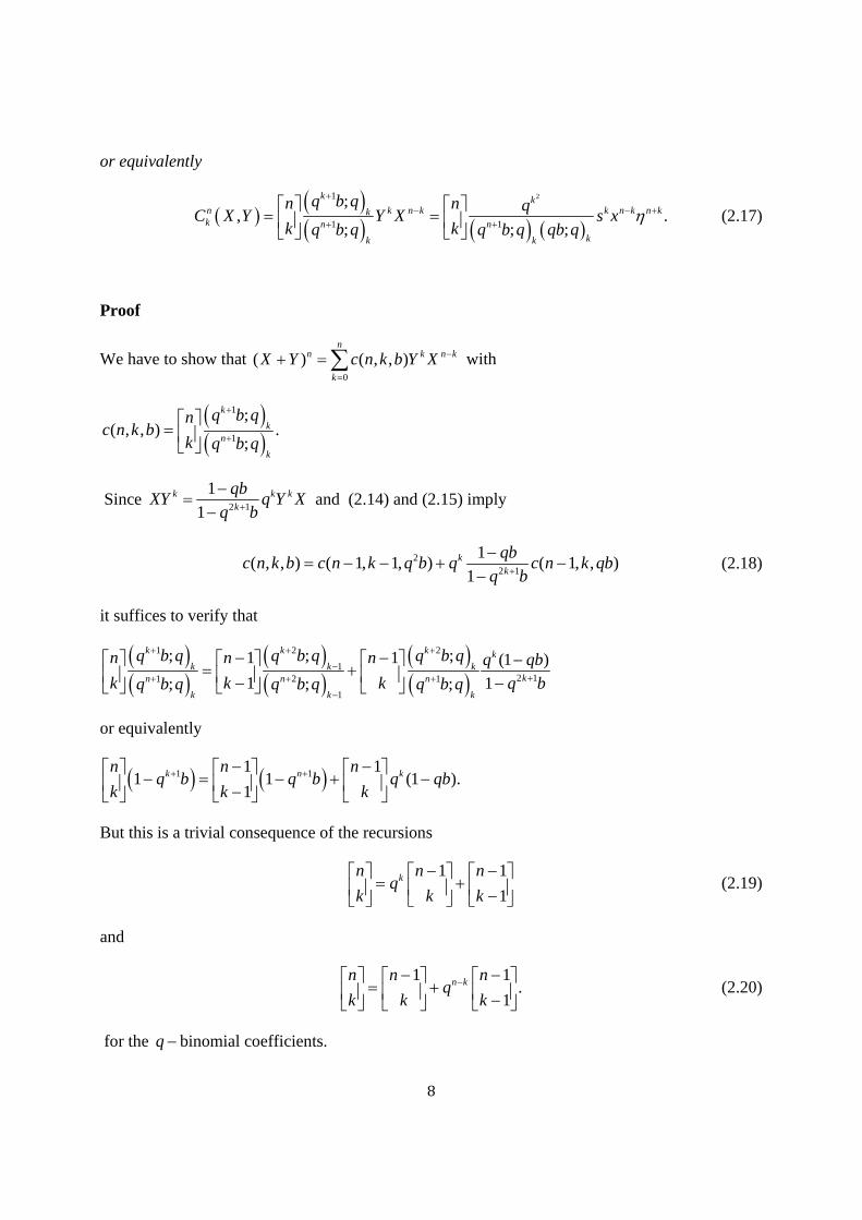
or equivalently
21
1 1
;, .
; ; ;
k kn k n k k n k n kkk n n
kk k
q b qn n qC X Y Y X s x
k kq b q q b q qb q
(2.17)
Proof
We have to show that 0
( ) ( , , )n
n k n k
k
X Y c n k b Y X
with
1
1
;( , , ) .
;
k
kn
k
q b qnc n k b
k q b q
Since 2 1
1
1k k k
k
qbXY q Y X
q b
and (2.14) and (2.15) imply
22 1
1( , , ) ( 1, 1, ) ( 1, , )
1k
k
qbc n k b c n k q b q c n k qb
q b
(2.18)
it suffices to verify that
1 2 2
12 11 2 1
1
; ; ;1 1 (1 )
1 1; ; ;
k k k kk k k
kn n n
k k k
q b q q b q q b qn n n q qb
k k k q bq b q q b q q b q
or equivalently
1 11 11 1 (1 ).
1k n kn n n
q b q b q qbk k k
But this is a trivial consequence of the recursions
1 1
1kn n n
qk k k
(2.19)
and
1 1
.1
n kn n nq
k k k
(2.20)
for the q binomial coefficients.
9
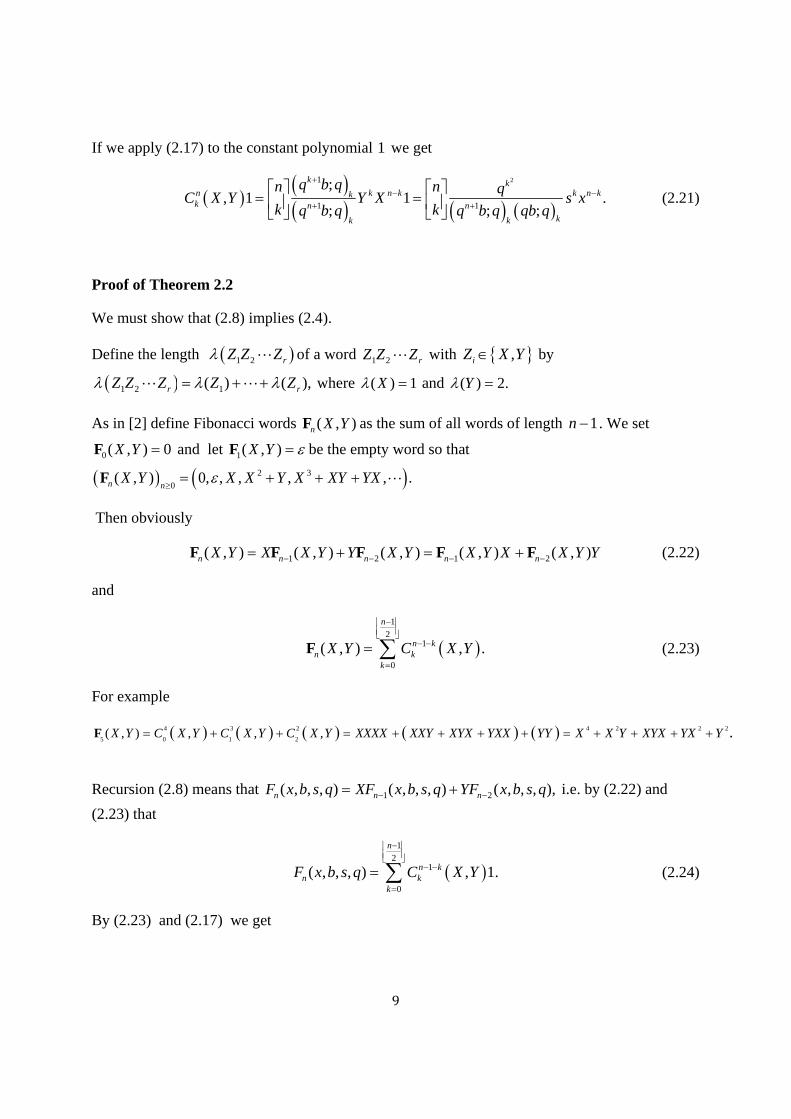
If we apply (2.17) to the constant polynomial 1 we get
21
1 1
;, 1 1 .
; ; ;
k kn k n k k n kkk n n
kk k
q b qn n qC X Y Y X s x
k kq b q q b q qb q
(2.21)
Proof of Theorem 2.2
We must show that (2.8) implies (2.4).
Define the length 1 2 rZ Z Z of a word 1 2 rZ Z Z with ,iZ X Y by
1 2 1( ) ( ),r rZ Z Z Z Z where ( ) 1X and ( ) 2.Y
As in [2] define Fibonacci words ( , )n X YF as the sum of all words of length 1n . We set
0( , ) 0X Y F and let 1( , )X Y F be the empty word so that
2 3
0( , ) 0, , , , , .n nX Y X X Y X XY YX
F
Then obviously
1 2 1 2( , ) ( , ) ( , ) ( , ) ( , )n n n n nX Y X X Y Y X Y X Y X X Y Y F F F F F (2.22)
and
1
21
0
( , ) , .
n
n kn k
k
X Y C X Y
F (2.23)
For example
4 3 2 4 2 2 2
5 0 1 2( , ) , , , .X Y C X Y C X Y C X Y XXXX XXY XYX YXX YY X X Y XYX YX Y F
Recursion (2.8) means that 1 2( , , , ) ( , , , ) ( , , , ),n n nF x b s q XF x b s q YF x b s q i.e. by (2.22) and
(2.23) that
1
21
0
( , , , , 1) .
n
n kk
knF x b s q C X Y
(2.24)
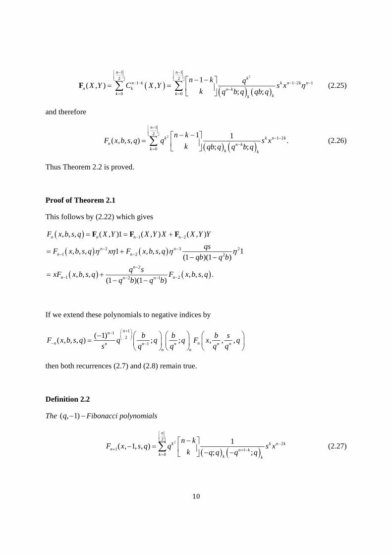
By (2.23) and (2.17) we get
10
21 1
1 2 12 2
1
0 0
( , ) ,1
; ;
kk n k n
n
n n
n kn k
kkk k
k
n k qs x
k qX Y C X
bY
b q q q
F (2.25)
and therefore
2
1
21 2
0
1 1( , , , ) .
; ;
n
k k n kn n k
k k k
n kF x b s q q s x
k qb q q b q
(2.26)
Thus Theorem 2.2 is proved.
Proof of Theorem 2.1
This follows by (2.22) which gives
1 2
2 3 21 2 2
2
1 22 1
, , , ( , )1 ( , ) ( , )
, , , 1 , , , 1(1 )(1 )
, , , , , , .(1 )(1 )
n n n n
n nn n
n
n nn n
F x b s q X Y X Y X X Y Y
qsF x b s q x F x b s q
qb q b
q sxF x b s q F x b s q
q b q b
F F F
If we extend these polynomials to negative indices by
112
1
( 1)( , , , ) ; ; , , ,
nn
n nn n n n nn n
b b b sF x b s q q q q F x q
s q q q q
then both recurrences (2.7) and (2.8) remain true.
Definition 2.2
The ( , 1)q Fibonacci polynomials
22
21 1
0
1( , 1, , )
; ;
n
k k n kn n k
k k k
n kF x s q q s x
k q q q q
(2.27)
11
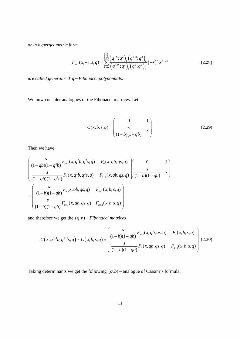
or in hypergeometric form
2 1 222
1 2 2 2 20
; ;( , 1, , )
; ;
nn n
k n kk kn n
kk k
q q q qF x s q s x
q q q q
(2.28)
are called generalized q Fibonacci polynomials.
We now consider analogues of the Fibonacci matrices. Let
0 1
( , , , ) .
(1 )(1 )
C x b s q sx
b qb
(2.29)
Then we have
2 212
2 212
1
1 2
( , , , ) ( , , , ) 0 1(1 )(1 )
( , , , ) ( , , , ) (1 )(1 )(1 )(1 )
( , , , ) ( , , , )(1 )(1 )
( , , , ) ( , ,(1 )(1 )
n n
n n
n n
n n
sF x q b q s q F x qb qs q
qb q bs
xsF x q b q s q F x qb qs q b qb
qb q b
sF x qb qs q F x b s q
b qb
sF x qb qs q F x b
b qb
, )s q
and therefore we get the ( , )q b Fibonacci matrices
1
1 1
1
( , , , ) ( , , , )(1 )(1 )
, , , , , , .
( , , , ) ( , , , )(1 )(1 )
n nn n
n n
sF x qb qs q F x b s q
b qbC x q b q s q C x b s q
sF x qb qs q F x b s q
b qb
(2.30)
Taking determinants we get the following ( , )q b analogue of Cassini’s formula.
12
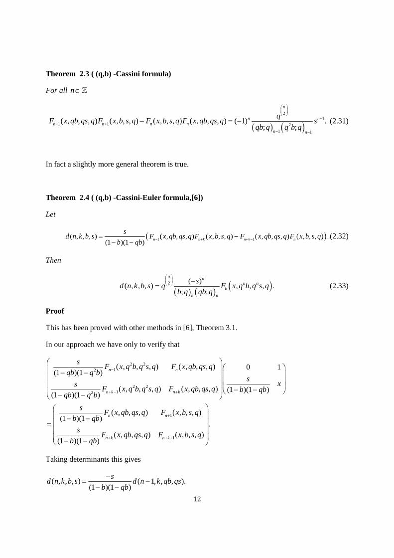
Theorem 2.3 ( (q,b) -Cassini formula)
For all n
21
1 1 2
1 1
( , , , ) ( , , , ) ( , , , ) ( , , , ) ( 1) .; ;
n
n nn n n n
n n
qF x qb qs q F x b s q F x b s q F x qb qs q s
qb q q b q
(2.31)
In fact a slightly more general theorem is true.
Theorem 2.4 ( (q,b) -Cassini-Euler formula,[6])
Let
1 1( , , , ) ( , , , ) ( ,( , , , , ) ( , , ,, ) .(1 )(1
))
n n k n k nd n k bs
F x qb qs q F x b s q F x qb qs q F x b s qb q
sb
(2.32)
Then
2 ( )
( , , , ) , , , .; ;
n nn n
k
n n
sd n k b s q F x q b q s q
b q qb q
(2.33)
Proof
This has been proved with other methods in [6], Theorem 3.1.
In our approach we have only to verify that
2 212
2 212
1
( , , , ) ( , , , ) 0 1(1 )(1 )
( , , , ) ( , , , ) (1 )(1 )(1 )(1 )
( , , , ) ( , , , )(1 )(1 )
( , , , )(1 )(1 )
n n
n k n k
n n
n k n k
sF x q b q s q F x qb qs q
qb q bs
xsF x q b q s q F x qb qs q b qb
qb q b
sF x qb qs q F x b s q
b qb
sF x qb qs q F
b qb
1
.
( , , , )x b s q
Taking determinants this gives
( , , , ) ( 1, , , ).(1 )(1 )
sd n k b s d n k qb qs
b qb
13
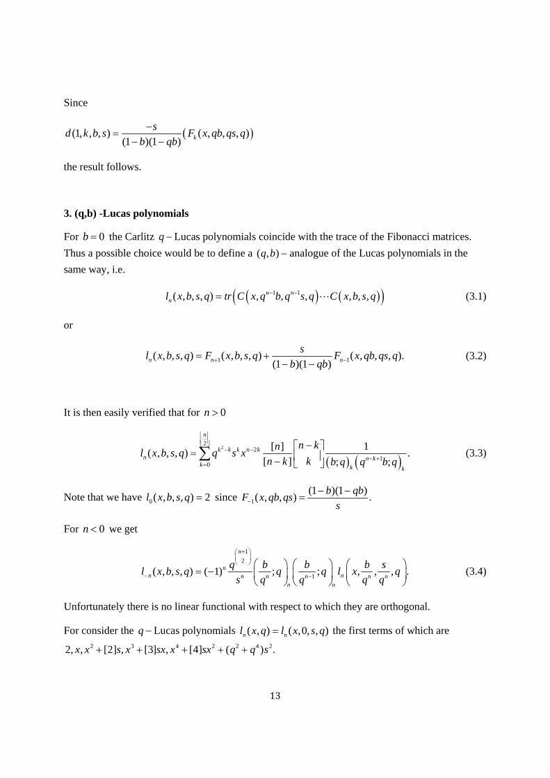
Since
( , , , )(1 )(1 )
(1, , , ) k
sFd k x qb qs q
b bb
qs
the result follows.
3. (q,b) -Lucas polynomials
For 0b the Carlitz q Lucas polynomials coincide with the trace of the Fibonacci matrices.
Thus a possible choice would be to define a ( , )q b analogue of the Lucas polynomials in the
same way, i.e.
1 1, , , , , ,( , , , ) n nn C x q b q sl x b q C x b sq t qs r (3.1)
or
1 1( , , , ) ( , , , ) ( , , , ).(1 )(1 )n n n
sl x b s q F x b s q F x qb qs q
b qb
(3.2)
It is then easily verified that for 0n
22
2
10
[ ] 1( , , , ) .
[ ] ; ;
n
k k k n kn n k
k k k
n knl x b s q q s x
kn k b q q b q
(3.3)
Note that we have 0( , , , ) 2l x b s q since 1
(1 )(1 )( , , ) .
b qbF x qb qs
s
For 0n we get
1
2
1( , , , ) ( 1) ; ; , , , .
n
nn nn n n n n
n n
q b b b sl x b s q q q l x q
s q q q q
(3.4)
Unfortunately there is no linear functional with respect to which they are orthogonal.
For consider the q Lucas polynomials ( , ) ( ,0, , )n nl x q l x s q the first terms of which are 2 3 4 2 2 4 22, , [2] , [3] , [4] ( ) .x x s x sx x sx q q s
14
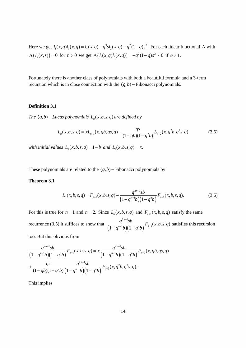
Here we get 3 2 21 3 4 2( , ) ( , ) ( , ) ( , ) (1 ) .l x q l x q l x q q sl x q q q s For each linear functional with
( , ) 0nl x s for 0n we get 2 21 3( , ) ( , ) (1 ) 0l x q l x q q q s if 1.q
Fortunately there is another class of polynomials with both a beautiful formula and a 3-term recursion which is in close connection with the ( , )q b Fibonacci polynomials.
Definition 3.1
The ( , )q b Lucas polynomials ( , , , )nL x b s q are defined by
2 21 22
( , , , ) ( , , , ) ( , , , )(1 )(1 )n n n
qsL x b s q xL x qb qs q L x q b q s q
qb q b
(3.5)
with initial values 0( , , , ) 1L x b s q b and 1( , , , ) .L x b s q x
These polynomials are related to the ( , )q b Fibonacci polynomials by
Theorem 3.1
2 1
1 11( , , , ) ( , , , ) ( , , , ).
1 1
n
n n nn n
q sbL x b s q F x b s q F x b s q
q b q b
(3.6)
For this is true for 1n and 2.n Since ( , , , )nL x b s q and 1( , , , )nF x b s q satisfy the same
recurrence (3.5) it suffices to show that 2 1
11( , , , )
1 1
n
nn n
q sbF x b s q
q b q b
satisfies this recursion
too. But this obvious from
2 1 2 1
1 21 1
2 12 2
312
( , , , ) ( , , , )1 1 1 1
( , , ,(1 )
).1 1(1 )
n n
n nn n n n
n
nn n
q sb q sbF x b s q x F x qb qs q
q b q b q b q b
q sbF x q b q s q
q b q b
qs
qb q b
This implies
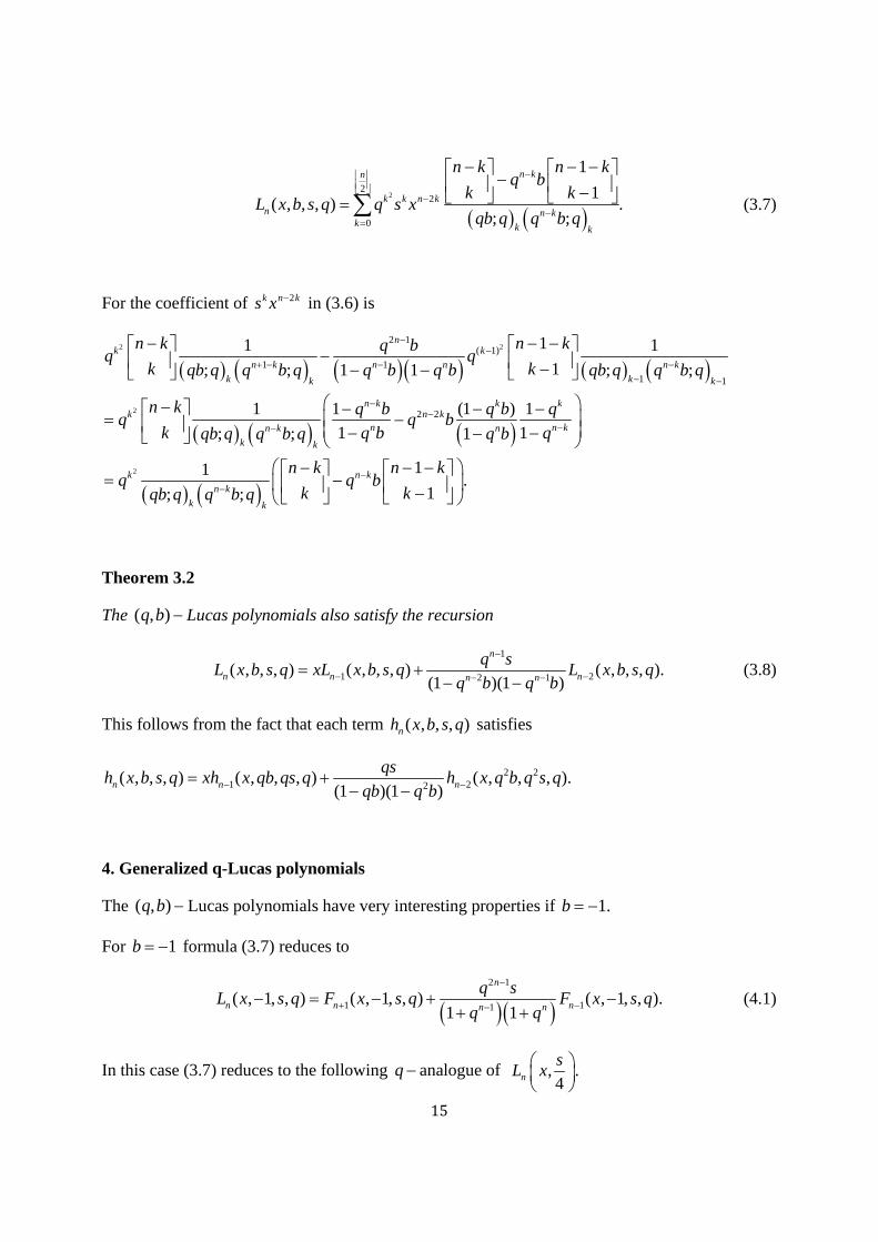
15
22
2
0
1
1( , , , ) .
; ;
n kn
k k n kn n k
k k k
n k n kq b
k kL x b s q q s x
qb q q b q
(3.7)
For the coefficient of 2k n ks x in (3.6) is
2 2
2
2
2 1( 1)
1 1
1 1
2 2
11 1
1; ; 1 1 ; ;
1 1 (1 ) 1
1 1; ; 1
1
; ;
nk k
n k n n n k
k kk k
n k k kk n k
n n kn k n
k k
k n k
n k
k k
n k n kq bq q
k kqb q q b q q b q b qb q q b q
n k q b q b qq q b
k q b qqb q q b q q b
n k nq q b
kqb q q b q
1.
1
k
k
Theorem 3.2
The ( , )q b Lucas polynomials also satisfy the recursion
1
1 22 1( , , , ) ( , , , ) ( , , , ).
(1 )(1 )
n
n n nn n
q sL x b s q xL x b s q L x b s q
q b q b
(3.8)
This follows from the fact that each term ( , , , )nh x b s q satisfies
2 21 22
( , , , ) ( , , , ) ( , , , ).(1 )(1 )n n n
qsh x b s q xh x qb qs q h x q b q s q
qb q b
4. Generalized q-Lucas polynomials
The ( , )q b Lucas polynomials have very interesting properties if 1.b
For 1b formula (3.7) reduces to
2 1
1 11( , 1, , ) ( , 1, , ) ( , 1, , ).
1 1
n
n n nn n
q sL x s q F x s q F x s q
q q
(4.1)
In this case (3.7) reduces to the following q analogue of , .4n
sL x
16
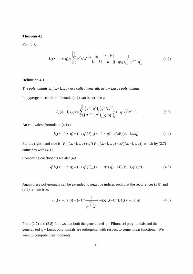
Theorem 4.1
For 0n
22
2
0
[ ] 1( , 1, , ) .
[ ] ; ;
n
k k n kn n k
k k k
n knL x s q q s x
kn k q q q q
(4.2)
Definition 4.1
The polynomials ( , 1, , )nL x s q are called generalized q Lucas polynomials.
In hypergeometric form formula (4.2) can be written as
2 1 222 2
2 2 2 2 20
; ;( , 1, , ) .
; ;
nn n
k n kk kn n
kk k
q q q qL x s q q s x
q q q q
(4.3)
An equivalent formula to (4.1) is
1( , 1, , ) (1 ) ( , 1, , ) ( , 1, , ).n nn n nL x s q q F x s q q xF x s q (4.4)
For the right-hand side is 1 1( , 1, , ) ( , 1, , ) ( , 1, , )nn n nF x s q q F x s q xF x s q which by (2.7)
coincides with (4.1).
Comparing coefficients we also get
2 21( , 1, , ) (1 ) ( , 1, , ) ( , 1, , ).n n
n n nq L x s q q F x q s q xF x q s q (4.5)
Again these polynomials can be extended to negative indices such that the recurrences (3.8) and (3.5) remain true:
1
2
1( , 1, , ) ( 1) ( ; ) ( 1; ) ( , 1, , ).n
n n n nn
n
L x s q q q q L x s q
q s
(4.6)
From (2.7) and (3.8) follows that both the generalized q Fibonacci polynomials and the
generalized q Lucas polynomials are orthogonal with respect to some linear functional. We
want to compute their moments.
17
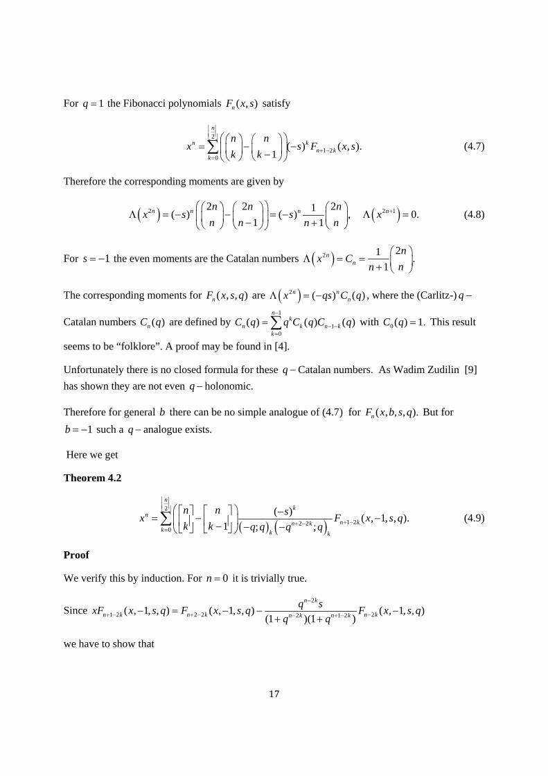
For 1q the Fibonacci polynomials ( , )nF x s satisfy
2
1 20
( ) ( , ).1
n
n kn k
k
n nx s F x s
k k
(4.7)
Therefore the corresponding moments are given by
2 2 12 2 21( ) ( ) , 0.
1 1n n n nn n n
x s s xn n nn
(4.8)
For 1s the even moments are the Catalan numbers 2 21.
1n
n
nx C
nn
The corresponding moments for ( , , )nF x s q are 2 ( ) ( )n nnx qs C q , where the (Carlitz-) q
Catalan numbers ( )nC q are defined by 1
10
( ) ( ) ( )n
kn k n k
k
C q q C q C q
with 0( ) 1.C q This result
seems to be “folklore”. A proof may be found in [4].
Unfortunately there is no closed formula for these q Catalan numbers. As Wadim Zudilin [9]
has shown they are not even q holonomic.
Therefore for general b there can be no simple analogue of (4.7) for ( , , , ).nF x b s q But for
1b such a q analogue exists.
Here we get
Theorem 4.2
2
1 22 20
( )( , 1, , ).
1 ; ;
nk
nn kn k
k k k
n n sx F x s q
k k q q q q
(4.9)
Proof
We verify this by induction. For 0n it is trivially true.
Since 2
1 2 2 2 22 1 2( , 1, , ) ( , 1, , ) ( , 1, , )
(1 )(1 )
n k
n k n k n kn k n k
q sxF x s q F x s q F x s q
q q
we have to show that
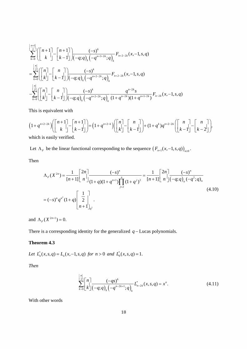
18
1
2
2 23 20
2
2 22 20
2
0
1 1 ( )( , 1, , )
1 ; ;
( )( , 1, , )
1 ; ;
( )
1
nk
n kn kk k k
nk
n kn kk k k
nk
k
n n sF x s q
k k q q q q
n n sF x s q
k k q q q q
n n s
k k
2
22 1 22 2( , 1, , )
(1 )(1 ); ;
n k
n kn k n kn k
k k
q sF x s q
q qq q q q
This is equivalent with
2 2 2 2 21 11 1 (1 ) ,
1 1 1 2n k n k k n kn n n n n n
q q q qk k k k k k
which is easily verified.
Let F be the linear functional corresponding to the sequence 1 0( , 1, , )n n
F x s q .
Then
2
2
22
1 2
2
2 21 ( ) 1 ( )( )
[ 1] [ 1] ; ( ; )(1 )(1 ) (1 )
1( ) (1 ) .2
1
n nn
F nn j nn
j
n n
q
n ns sX
n nn n q q q qq q q
s q qn
(4.10)
and 2 1( ) 0.nF X
There is a corresponding identity for the generalized q Lucas polynomials.
Theorem 4.3
Let * ( , , ) ( , 1, , )n nL x s q L x s q for 0n and *0( , , ) 1.L x s q
Then
2*
22 10
( )( , , ) .
; ;
nk
nn kn k
k k k
n qsL x s q x
k q q q q
(4.11)
With other words
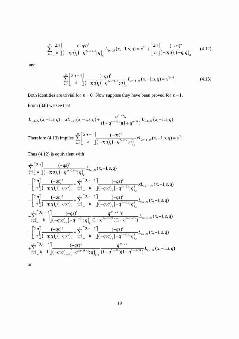
19
22 22 2 1
0
2 2( ) ( )( , 1, , )
; ;; ;
k nnn
n kn kk n nk k
n nqs qsL x s q x
k n q q q qq q q q
(4.12)
and
2 12 1 22 2 2
0
2 1 ( )( , 1, , ) .
; ;
knn
n kn kk k k
n qsL x s q x
k q q q q
(4.13)
Both identities are trivial for 0.n Now suppose they have been proved for 1.n
From (3.8) we see that
2
1 2 2 1 21 2 2( , 1, , ) ( , 1, , ) ( , 1, , )
(1 )(1 )
n k
n k n k n kn k n k
q sL x s q xL x s q L x s q
q q
Therefore (4.13) implies
22 1 22 2
0
2 1 ( )( , 1, , ) .
; ;
knn
n kn kk k k
n qsxL x s q x
k q q q q
Thus (4.12) is equivalent with
2 22 2 10
2 1 22 20
2 22 2
2 ( )( , 1, , )
; ;
2 2 1( ) ( )( , 1, , )
; ; ; ;
2 2 1( ) ( )
; ; ; ;
kn
n kn kk k k
n kn
n kn kkn n k k
n k
nn kn n k k
n qsL x s q
k q q q q
n nqs qsxL x s q
n kq q q q q q q q
n nqs qsL
n kq q q q q q q q
0
2 2 1
2 2 22 2 2 2 1 22 20
2 22 20
( , 1, , )
2 1 ( )( , 1, , )
(1 )(1 ); ;
2 2 1( ) ( )( , 1, , )
; ; ; ;
2 1 (
1
n
kk
k n kn
n kn k n kn kk k k
n kn
n kn kkn n k k
x s q
n qs q sL x s q
k q qq q q q
n nqs qsL x s q
n kq q q q q q q q
n
k
2 2
2 22 2 2 1 22 2 20 1 1
)( , 1, , )
(1 )(1 ); ;
k n kn
n kn k n kn kk k k
qs qL x s q
q qq q q q
or
20
2 22 2 10
2 22 20
2 2
2 2 22 2 20 1 1
2 ( )( , 1, , )
; ;
2 2 1( ) ( )( , 1, , )
; ; ; ;
2 1 ( )
1 (1 )(1; ;
kn
n kn kk k k
n kn
n kn kkn n k k
k n kn
n kn kk k k
n qsL x s q
k q q q q
n nqs qsL x s q
n kq q q q q q q q
n qs q
k q qq q q q
2 21 2( , 1, , )
) n kn kL x s q
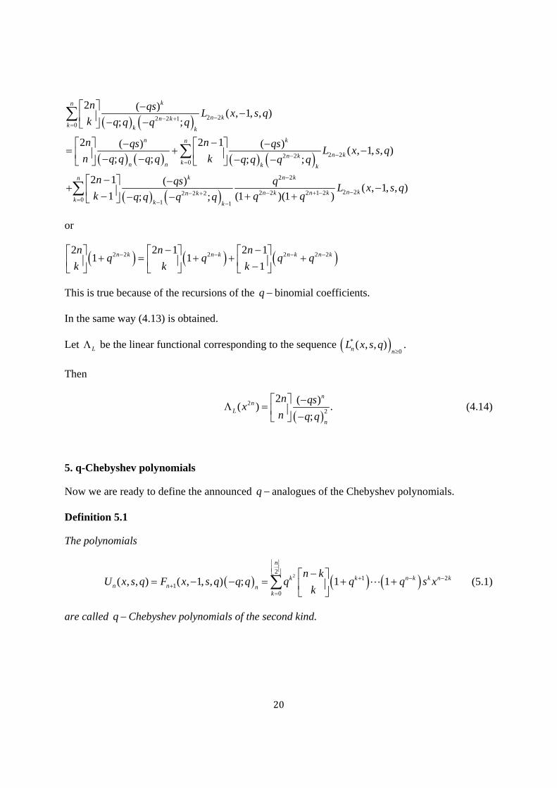
or
2 2 2 2 2 22 2 1 2 11 1
1n k n k n k n kn n n
q q q qk k k
This is true because of the recursions of the q binomial coefficients.
In the same way (4.13) is obtained.
Let L be the linear functional corresponding to the sequence *
0( , , ) .n n
L x s q
Then
22
2 ( )( ) .
;
nn
L
n
n qsx
n q q
(4.14)
5. q-Chebyshev polynomials
Now we are ready to define the announced q analogues of the Chebyshev polynomials.
Definition 5.1
The polynomials
22
21
1
0
( , , ) ( , 1, , ) 1; 1
n
k k n kn n n
k n k
k
n kU x s q F x s q q qq q sq x
k
(5.1)
are called q Chebyshev polynomials of the second kind.
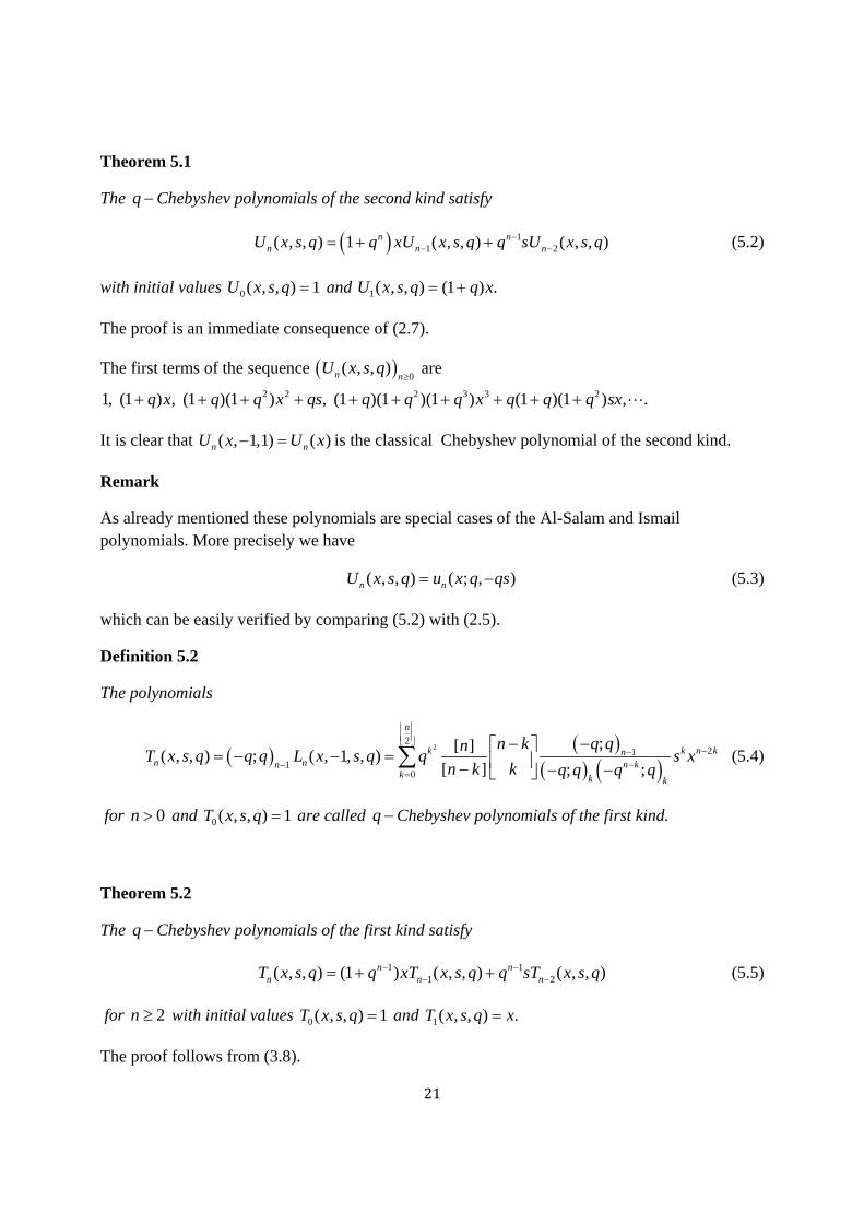
21
Theorem 5.1
The q Chebyshev polynomials of the second kind satisfy
11 2( , , ) 1 ( , , ) ( , , )n n
n n nU x s q q xU x s q q sU x s q (5.2)
with initial values 0( , , ) 1U x s q and 1( , , ) (1 ) .U x s q q x
The proof is an immediate consequence of (2.7).
The first terms of the sequence 0
( , , )n nU x s q
are
2 2 2 3 3 21, (1 ) , (1 )(1 ) , (1 )(1 )(1 ) (1 )(1 ) , .q x q q x qs q q q x q q q sx
It is clear that ( , 1,1) ( )n nU x U x is the classical Chebyshev polynomial of the second kind.
Remark
As already mentioned these polynomials are special cases of the Al-Salam and Ismail polynomials. More precisely we have
( , , ) ( ; , )n nU x s q u x q qs (5.3)
which can be easily verified by comparing (5.2) with (2.5).
Definition 5.2
The polynomials
2
1
212
0
[ ]
[
;( , , ) ; ( , 1, , )
; ;]n
n n n k
n
k k k
kn
k k
nn knq s x
kn
q qT x s q q q L x s q
q q q qk
(5.4)
for 0n and 0( , , ) 1T x s q are called q Chebyshev polynomials of the first kind.
Theorem 5.2
The q Chebyshev polynomials of the first kind satisfy
1 11 2( , , ) (1 ) ( , , ) ( , , )n n
n n nT x s q q xT x s q q sT x s q (5.5)
for 2n with initial values 0( , , ) 1T x s q and 1( , , ) .T x s q x
The proof follows from (3.8).
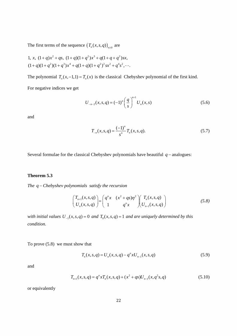
22
The first terms of the sequence 0
( , , )n nT x s q
are
2 2 3 2
2 3 4 2 2 2 4 2
1, , (1 ) , (1 )(1 ) (1 ) ,
(1 )(1 )(1 ) (1 )(1 ) , .
x q x qs q q x q q q sx
q q q x q q q sx q s
The polynomial ( , 1,1) ( )n nT x T x is the classical Chebyshev polynomial of the first kind.
For negative indices we get
1
2 ( , , ) ( 1) ( , )n
nn n
qU x s q U x s
s
(5.6)
and
( 1)
( , , ) ( , , ).n
n nnT x s q T x s q
s
(5.7)
Several formulae for the classical Chebyshev polynomials have beautiful q analogues:
Theorem 5.3
The q Chebyshev polynomials satisfy the recursion
2 2
1
1
( , , ) ( , , )( )
( , , ) ( , , )1
nn n
nn n
T x s q T x s qq x x qs
U x s q U x s qq x
(5.8)
with initial values 1( , , ) 0U x s q and 0( , , ) 1T x s q and are uniquely determined by this
condition.
To prove (5.8) we must show that
1( , , ) ( , , ) ( , , )nn n nT x s q U x s q q xU x s q (5.9)
and
2 21 1( , , ) ( , , ) ( ) ( , , )n
n n nT x s q q xT x s q x qs U x q s q (5.10)
or equivalently
23
2 21(1 ) ( , 1, , ) ( , 1, , ) ( ) ( , 1, , ).n n
n n nq L x s q q xL x s q x qs F x q s q (5.11)
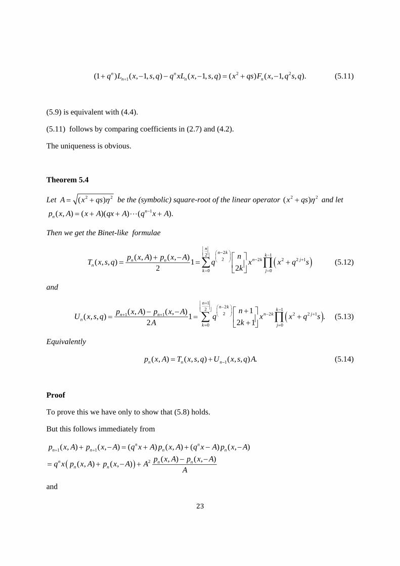
(5.9) is equivalent with (4.4).
(5.11) follows by comparing coefficients in (2.7) and (4.2).
The uniqueness is obvious.
Theorem 5.4
Let 2 2( )A x qs be the (symbolic) square-root of the linear operator 2 2( )x qs and let 1( , ) ( )( ) ( ).n
np x A x A qx A q x A
Then we get the Binet-like formulae
22 1
2 2 2 2 1
0 0
( , ) ( , )( , , ) 1
22
nn k
kn k jn n
nk j
np x A p x AT x s q q x x q s
k
(5.12)
and
1
22 12 2 2 2 11 1
0 0
1( , ) ( , )( , , ) 1 .
2 12
nn k
kn k jn n
nk j
np x A p x AU x s q q x x q s
kA
(5.13)
Equivalently
1( , ) ( , , ) ( , , ) .n n np x A T x s q U x s q A (5.14)
Proof
To prove this we have only to show that (5.8) holds.
But this follows immediately from
1 1
2
( , ) ( , ) ( ) ( , ) ( ) ( , )
( , ) ( , )( , ) ( , )
n nn n n n
n n nn n
p x A p x A q x A p x A q x A p x A
p x A p x Aq x p x A p x A A
A
and
24
1 1( , ) ( , ) ( ) ( , ) ( ) ( , )
( , ) ( , )( , ) ( , ).
n nn n n n
n n nn n
p x A p x A q x A p x A q x A p x A
A Ap x A p x A
q x p x A p x AA
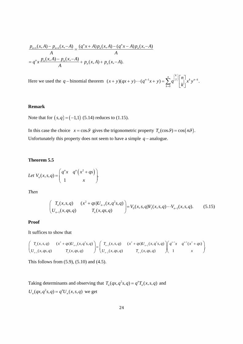
Here we used the q binomial theorem 21
0
( )( ) ( ) .k
nn k n k
k
nx y qx y q x y q x y
k
Remark
Note that for , 1,1s q (5.14) reduces to (1.15).
In this case the choice cosx gives the trigonometric property (cos ) cos .nT n
Unfortunately this property does not seem to have a simple q analogue.
Theorem 5.5
Let 2
( , , ) .1
n n
n
q x q x qsV x s q
x
Then
2 2
10 1 1
1
( , , ) ( ) ( , , )( , , ) ( , , ) ( , , ).
( , , ) ( , , )n n
n
n n
T x s q x qs U x q s qV x s q V x s q V x s q
U x qs q T x qs q
(5.15)
Proof
It suffices to show that
2 2 2 2 1 1 2
1 1 2
1 2 1
( , , ) ( ) ( , , ) ( , , ) ( ) ( , , ) ( ).
( , , ) ( , , ) ( , , ) ( , , ) 1
n n
n n n n
n n n n
T x s q x qs U x q s q T x s q x qs U x q s q q x q x qs
U x qs q T x qs q U x qs q T x qs q x
This follows from (5.9), (5.10) and (4.5).
Taking determinants and observing that 2( , , ) ( , , )nn nT qx q s q q T x s q and
2( , , ) ( , , )nn nU qx q s q q U x s q we get
25
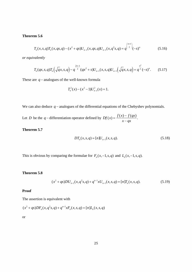
Theorem 5.6
1
22 21 1( , , ) ( , , ) ( ) ( , , ) ( , , ) ( )
n
nn n n nT x s q T x qs q x qs U x qs q U x q s q q s
(5.16)
or equivalently
22 1
22 21 1( , , ) , , ( ) ( , , ) , , ( ) .
n nn
n n n nT qx s q T qx s q q qx s U x s q U qx s q q s
(5.17)
These are q analogues of the well-known formula
2 2 21( ) ( 1) ( ) 1.n nT x x U x
We can also deduce q analogues of the differential equations of the Chebyshev polynomials.
Let D be the q differentiation operator defined by ( ) ( )
( ) .f x f qx
Df xx qx
Theorem 5.7
1( , , ) [ ] ( , , ).n nDT x s q n U x s q (5.18)
This is obvious by comparing the formulae for ( , 1, , )nF x s q and ( , 1, , ).nL x s q
Theorem 5.8
2 2 11 1( ) ( , , ) ( , , ) [ ] ( , , ).n
n n nx qs DU x q s q q xU x s q n T x s q (5.19)
Proof
The assertion is equivalent with
2 2 1( ) ( , , ) ( , , ) [ ] ( , , )nn n nx qs DF x q s q q xF x s q n L x s q
or
26
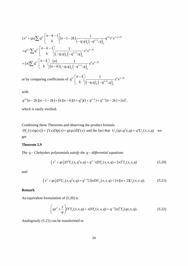
2
2
2
2 2 2 2
1 2
2
1 1( ) [ 1 2 ]
; ;
1 1
; ;
[ ] 1[ ]
[ ] ; ;
k k k n k
n k
k k
n k k n k
n k
k k
k k n k
n k
k k
n kx qs q n k q s x
k q q q q
n kq q s x
k q q q q
n k nn q s x
k n k q q q q
or by comparing coefficients of
2 21
; ;k k n k
n k
k k
n kq s x
k q q q q
with
2 1 2[ 2 ][ 1 2 ] [ ][ ](1 )(1 ) [ 2 ] [ ] ,k k n k nq n k n k k n k q q q n k n
which is easily verified.
Combining these Theorems and observing the product formula
( ) ( ) ( ) ( ) ( ) ( )D f x g x f x Dg x g qx Df x and the fact that 2( , , ) ( , , )nn nU qx q s q q U x s q we
get
Theorem 5.9
The q Chebyshev polynomials satisfy the q differential equations
2 2 2 1 2( , , ) ( , , ) [ ] ( , , )nn n nx qs D T x q s q q xDT x s q n T x s q (5.20)
and
2 2 2 1( , , ) [3] ( , , ) [ ][ 2] ( , , ).nn n nx qs D U x q s q q xDU x s q n n U x s q (5.21)
Remark
An equivalent formulation of (5.20) is
2 2 2( , , ) ( , , ) [ ] ( , , ).nn n n
sqx D T x s q xDT x s q q n T qx s q
q
(5.22)
Analogously (5.21) can be transformed to
27
3 2 2 ( , , ) [3] ( , , ) [ ][ 2] ( , , ).nn n n
sq x D U x s q xDU x s q q n n U qx s q
q
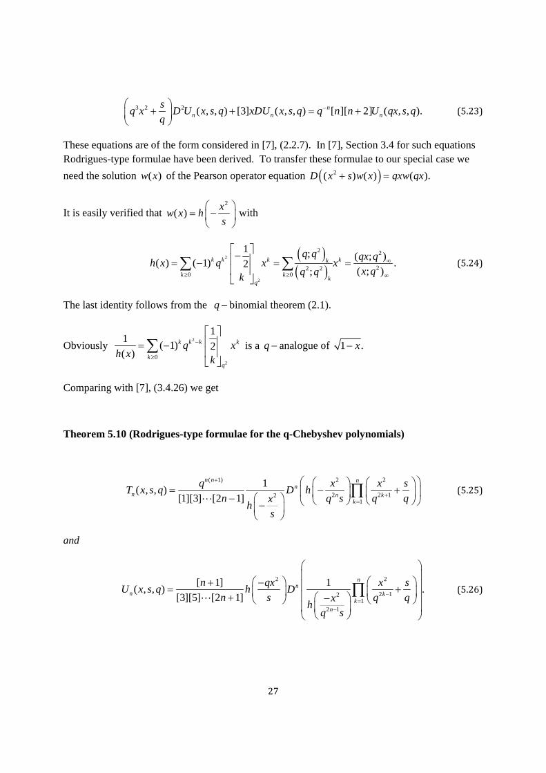
(5.23)
These equations are of the form considered in [7], (2.2.7). In [7], Section 3.4 for such equations Rodrigues-type formulae have been derived. To transfer these formulae to our special case we
need the solution ( )w x of the Pearson operator equation 2( ) ( ) ( ).D x s w x qxw qx
It is easily verified that 2
( )x
w x hs
with
2
2
2 2
22 20 0
1 ; ( ; )( ) ( 1) .2
( ; );k k k kk
k kk
q
q q qx qh x q x x
x qq qk
(5.24)
The last identity follows from the q binomial theorem (2.1).
Obviously 2
20
11
( 1) 2( )
k k k k
kq
q xh x
k
is a q analogue of 1 .x
Comparing with [7], (3.4.26) we get
Theorem 5.10 (Rodrigues-type formulae for the q-Chebyshev polynomials)
( 1) 2 2
2 2 121
1( , , )
[1][3] [2 1]
n n nn
n n kk
q x x sT x s q D h
n q s q qxh
s
(5.25)
and
2 2
2 121
2 1
[ 1] 1( , , ) .
[3][5] [2 1]
nn
n kk
n
n qx x sU x s q h D
n s q qxh
q s
(5.26)
28
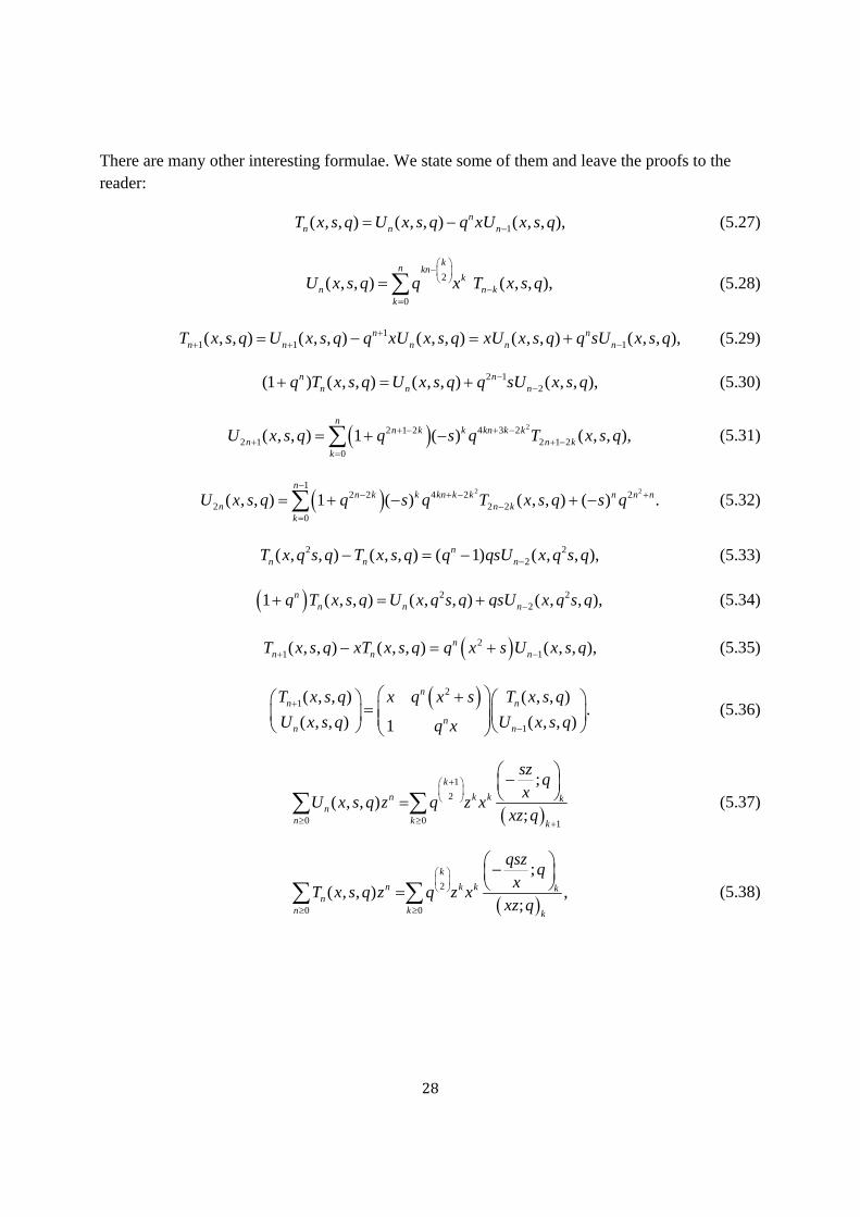
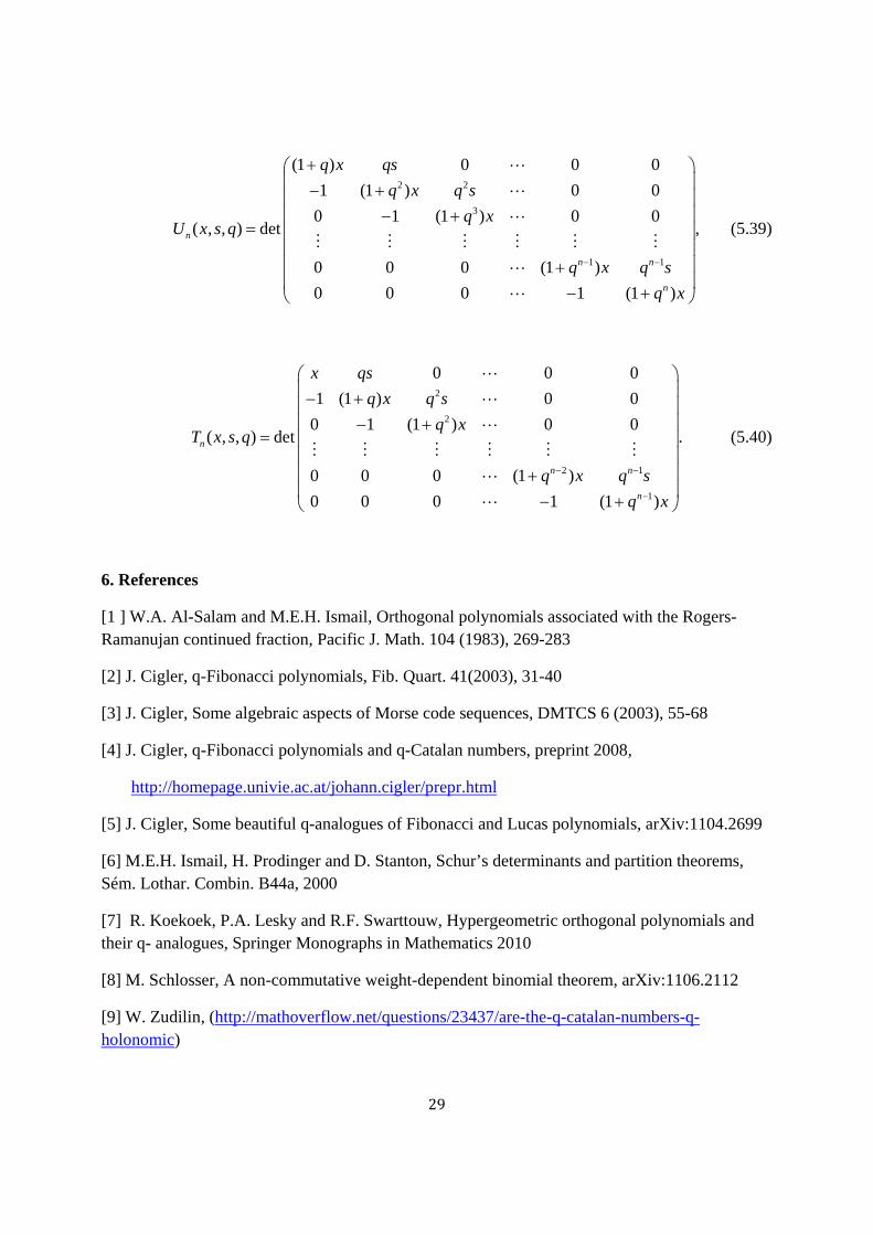
There are many other interesting formulae. We state some of them and leave the proofs to the reader:
1( , , ) ( , , ) ( , , ),nn n nT x s q U x s q q xU x s q (5.27)
2
0
( , , ) ( , , ),k
n knk
n n kk
U x s q q x T x s q
(5.28)
1
1 1 1( , , ) ( , , ) ( , , ) ( , , ) ( , , ),n nn n n n nT x s q U x s q q xU x s q xU x s q q sU x s q (5.29)
2 12(1 ) ( , , ) ( , , ) ( , , ),n n
n n nq T x s q U x s q q sU x s q (5.30)
22 1 2 4 3 2
2 1 2 1 20
( , , ) 1 ( ) ( , , ),n
n k k kn k kn n k
k
U x s q q s q T x s q
(5.31)
2 21
2 2 4 2 22 2 2
0
( , , ) 1 ( ) ( , , ) ( ) .n
n k k kn k k n n nn n k
k
U x s q q s q T x s q s q
(5.32)
2 22( , , ) ( , , ) ( 1) ( , , ),n
n n nT x q s q T x s q q qsU x q s q (5.33)
2 221 ( , , ) ( , , ) ( , , ),n
n n nq T x s q U x q s q qsU x q s q (5.34)
21 1( , , ) ( , , ) ( , , ),n
n n nT x s q xT x s q q x s U x s q (5.35)
2
1
1
( , , ) ( , , ).
( , , ) ( , , )1
nn n
nn n
T x s q x q x s T x s q
U x s q U x s qq x
(5.36)
1
2
0 0 1
;( , , )
;
k
n k k kn
n k k
szq
xU x s q z q z x
xz q
(5.37)
2
0 0
;( , , ) ,
;
k
n k k kn
n k k
qszq
xT x s q z q z x
xz q
(5.38)
29
2 2
3
1 1
(1 ) 0 0 0
1 (1 ) 0 0
0 1 (1 ) 0 0( , , ) det ,
0 0 0 (1 )
0 0 0 1 (1 )
n
n n
n
q x qs
q x q s
q xU x s q
q x q s
q x
(5.39)
2
2
2 1
1
0 0 0
1 (1 ) 0 0
0 1 (1 ) 0 0( , , ) det .
0 0 0 (1 )
0 0 0 1 (1 )
n
n n
n
x qs
q x q s
q xT x s q
q x q s
q x
(5.40)
6. References
[1 ] W.A. Al-Salam and M.E.H. Ismail, Orthogonal polynomials associated with the Rogers- Ramanujan continued fraction, Pacific J. Math. 104 (1983), 269-283
[2] J. Cigler, q-Fibonacci polynomials, Fib. Quart. 41(2003), 31-40
[3] J. Cigler, Some algebraic aspects of Morse code sequences, DMTCS 6 (2003), 55-68
[4] J. Cigler, q-Fibonacci polynomials and q-Catalan numbers, preprint 2008,
http://homepage.univie.ac.at/johann.cigler/prepr.html
[5] J. Cigler, Some beautiful q-analogues of Fibonacci and Lucas polynomials, arXiv:1104.2699
[6] M.E.H. Ismail, H. Prodinger and D. Stanton, Schur’s determinants and partition theorems, Sém. Lothar. Combin. B44a, 2000
[7] R. Koekoek, P.A. Lesky and R.F. Swarttouw, Hypergeometric orthogonal polynomials and their q- analogues, Springer Monographs in Mathematics 2010
[8] M. Schlosser, A non-commutative weight-dependent binomial theorem, arXiv:1106.2112
[9] W. Zudilin, (http://mathoverflow.net/questions/23437/are-the-q-catalan-numbers-q- holonomic)