Fourier series and Chebyshev polynomials applied to real

I S S N 0 1 8 8 - 6 2 6 6

Vol. 26 (NE-3) Redes de Agua y Drenaje Diciembre 2016 74

Fourier series and Chebyshev polynomials applied to real-time water demand forecasting

ABSTRACTRelevance of water demand forecasting increases with complexity of water supply systems. Several methods for water demand forecasting have been proposed in literature, mostly based on time-series analysis and machine learning, the later needing more detailed study of involved variables and choice of the best configuration to produce significant results. As an alternative to use of machine learning methods, this work presents two known meth-ods of data approximation, namely, discrete Fourier series and Chebyshev polynomials, to real-time demand forecasting, through real-time updating of some adjustable coefficients. A real district of a water supply system is analyzed using these methods, showing a good approximation between measured and forecasted values. The most interesting point of ap-plication is agility of calculation and the fact that there is no need to have information on factors influencing water demand.

RESUMENLa importancia de la previsión de la demanda de agua aumenta con la complejidad de los sistemas de abastecimiento de agua. Muchos métodos de predicción de demanda de agua, básicamente fundados en el análisis de series temporales y en mecanismos de regresión ba-sados en métodos de aprendizaje automático, han sido propuestos en la literatura. Los últimos necesitan de un estudio detallado de las variables involucradas y de la elección de la mejor arquitectura para la producción de resultados relevantes. Ese trabajo propone como alternativa aplicar dos métodos conocidos de aproximación de datos, a saber, las series discretas de Fourier y los polinomios de Chebyshev, a la previsión de demanda en tiempo real con actualización instantánea de los coeficientes ajustables en cada una de las funciones. Para contrastar la metodología propuesta se analizó un sector de una red real de abastecimiento de agua. Los resultados obtenidos muestran una buena aproximación entre los valores medidos y los predichos. El punto más interesante de la aplicación es la agilidad de cálculo y el hecho de que no hay necesidad de tener información de los factores que influyen en la demanda de agua.

* Faculdad de Engenharia Civil (FEC)-Unicamp, Campinas, São Paulo, Brasil. E-mail: [email protected]; [email protected]** FluIng-IMM, Universtitat Politècnica de València, Valencia, Spain. E-mail: [email protected]◊ Corresponding author.ˆ In memoriam: Rafael Pérez-García

Keywords: Water supply networks; real-time forecasting; water demand; Fourier series; Chebyshev polynomials.

Palabras clave:Redes de abastecimiento de agua; previsión en tiempo real; demanda de agua; series de Fourier; polinomios de Chebyshev.

Recibido: 6 de octubre de 2015Aceptado: 17 de octubre de 2016

Cómo citar:Brentan, B., Luvizotto Jr., E., Izquierdo, J., & Pérez-García, R. (2016). Fourier series and Che-byshev polynomials applied to real-time water demand forecasting. Acta Universitaria, 26(NE-3), 74-81. doi: 10.15174/au.2016.1022

doi: 10.15174/au.2016.1022

Series de Fourier y polinomios de Chebyshev aplicados a la previsión de demanda de agua en tiempo real

Bruno Brentan*◊, Edevar Luvizotto Jr.*, Joaquín Izquierdo**, Rafael Pérez-García**ˆ

INTRODUCTIONWater demand forecasting is needed not only for planning and development of new Water Supply Systems (WSSs), but also for operation and manage-ment of existent systems. Water companies should know behavior of demand in real time to safely operate their systems at the lowest cost. Usually, op-eration of WSSs use short time predictions to select optimal maneuvers for pumps and valves, with the advantage that real-time demand includes also water loses which can help with better management and, consequently, op-erational cost reduction (Alvisi, Franchini & Marinelli, 2007). Therefore, an accurate real-time water demand model helps operators identify leakages, once realized that water demand differs significantly from forecasted demand (Odan & Reis, 2012).


I S S N 0 1 8 8 - 6 2 6 6

Fourier series and Chebyshev polynomials applied to real-time water demand forecasting | Bruno Brentan, Edevar Luvizotto Jr., Joaquín Izquierdo, Rafael Pérez-García | pp. 74-81

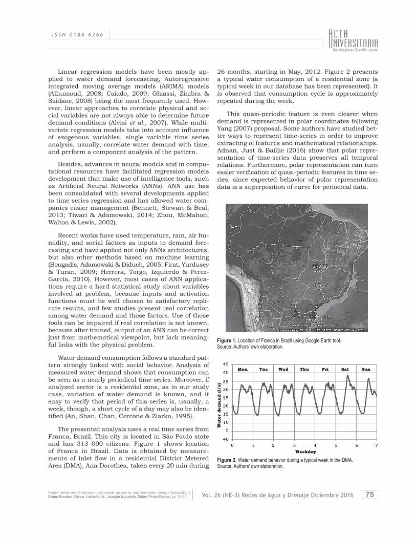
26 months, starting in May, 2012. Figure 2 presents a typical water consumption of a residential zone (a typical week in our database has been represented). It is observed that consumption cycle is approximately repeated during the week.

This quasi-periodic feature is even clearer when demand is represented in polar coordinates following Yang (2007) proposal. Some authors have studied bet-ter ways to represent time-series in order to improve extracting of features and mathematical relationships. Adnan, Just & Baillie (2016) show that polar repre-sentation of time-series data preserves all temporal relations. Furthermore, polar representation can turn easier verification of quasi-periodic features in time se-ries, since expected behavior of polar representation data is a superposition of curve for periodical data.

Linear regression models have been mostly ap-plied to water demand forecasting, Autoregressive integrated moving average models (ARIMA) models (Alhumoud, 2008; Caiado, 2009; Ghiassi, Zimbra & Saidane, 2008) being the most frequently used. How-ever, linear approaches to correlate physical and so-cial variables are not always able to determine future demand conditions (Alvisi et al., 2007). While multi-variate regression models take into account influence of exogenous variables, single variable time series analysis, usually, correlate water demand with time, and perform a component analysis of the pattern.

Besides, advances in neural models and in compu-tational resources have facilitated regression models development that make use of intelligence tools, such as Artificial Neural Networks (ANNs). ANN use has been consolidated with several developments applied to time series regression and has allowed water com-panies easier management (Bennett, Stewart & Beal, 2013; Tiwari & Adamowski, 2014; Zhou, McMahon, Walton & Lewis, 2002).

Recent works have used temperature, rain, air hu-midity, and social factors as inputs to demand fore-casting and have applied not only ANNs architectures, but also other methods based on machine learning (Bougadis, Adamowski & Diduch, 2005; Firat, Yurdusey & Turan, 2009; Herrera, Torgo, Izquierdo & Pérez-García, 2010). However, most cases of ANN applica-tions require a hard statistical study about variables involved at problem, because inputs and activation functions must be well chosen to satisfactory repli-cate results, and few studies present real correlation among water demand and those factors. Use of those tools can be impaired if real correlation is not known, because after trained, output of an ANN can be correct just from mathematical viewpoint, but lack meaning-ful links with the physical problem.

Water demand consumption follows a standard pat-tern strongly linked with social behavior. Analysis of measured water demand shows that consumption can be seen as a nearly periodical time series. Moreover, if analyzed sector is a residential zone, as in our study case, variation of water demand is known, and it easy to verify that period of this series is, usually, a week, though, a short cycle of a day may also be iden-tified (An, Shan, Chan, Cercone & Ziarko, 1995).

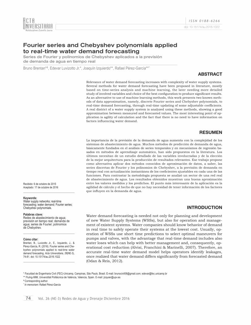
The presented analysis uses a real time series from Franca, Brazil. This city is located in São Paulo state and has 313 000 citizens. Figure 1 shows location of Franca in Brazil. Data is obtained by measure-ments of inlet flow in a residential District Metered Area (DMA), Ana Dorothea, taken every 20 min during

Figure 1. Location of Franca in Brazil using Google Earth tool. Source: Authors’ own elaboration.

Figure 2. Water demand behavior during a typical week in the DMA. Source: Authors’ own elaboration.

I S S N 0 1 8 8 - 6 2 6 6

Vol. 26 (NE-3) Redes de Agua y Drenaje Diciembre 2016 76 Fourier series and Chebyshev polynomials applied to real-time water demand forecasting | Bruno Brentan, Edevar Luvizotto Jr., Joaquín Izquierdo, Rafael Pérez-García | pp. 74-81

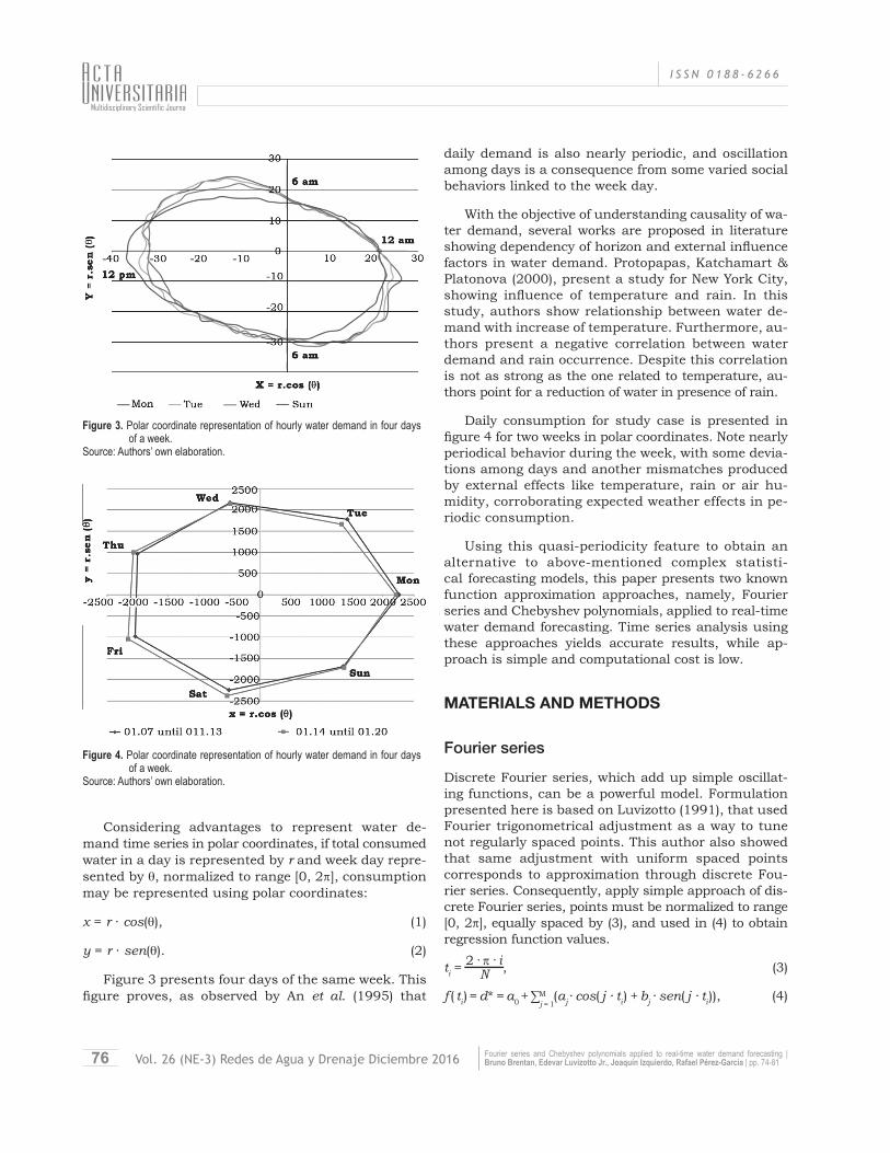
Considering advantages to represent water de-mand time series in polar coordinates, if total consumed water in a day is represented by r and week day repre-sented by θ, normalized to range [0, 2�], consumption may be represented using polar coordinates:

x = r ∙ cos(θ), (1)

y = r ∙ sen(θ). (2)

Figure 3 presents four days of the same week. This figure proves, as observed by An et al. (1995) that

daily demand is also nearly periodic, and oscillation among days is a consequence from some varied social behaviors linked to the week day.

With the objective of understanding causality of wa-ter demand, several works are proposed in literature showing dependency of horizon and external influence factors in water demand. Protopapas, Katchamart & Platonova (2000), present a study for New York City, showing influence of temperature and rain. In this study, authors show relationship between water de-mand with increase of temperature. Furthermore, au-thors present a negative correlation between water demand and rain occurrence. Despite this correlation is not as strong as the one related to temperature, au-thors point for a reduction of water in presence of rain.

Daily consumption for study case is presented in figure 4 for two weeks in polar coordinates. Note nearly periodical behavior during the week, with some devia-tions among days and another mismatches produced by external effects like temperature, rain or air hu-midity, corroborating expected weather effects in pe-riodic consumption.

Using this quasi-periodicity feature to obtain an alternative to above-mentioned complex statisti-cal forecasting models, this paper presents two known function approximation approaches, namely, Fourier series and Chebyshev polynomials, applied to real-time water demand forecasting. Time series analysis using these approaches yields accurate results, while ap-proach is simple and computational cost is low.

MATERIALS AND METHODS

Fourier seriesDiscrete Fourier series, which add up simple oscillat-ing functions, can be a powerful model. Formulation presented here is based on Luvizotto (1991), that used Fourier trigonometrical adjustment as a way to tune not regularly spaced points. This author also showed that same adjustment with uniform spaced points corresponds to approximation through discrete Fou-rier series. Consequently, apply simple approach of dis-crete Fourier series, points must be normalized to range [0, 2�], equally spaced by (3), and used in (4) to obtain regression function values.

ti = 2 · � · i

N , (3)

f ( ti) = d* = a0 + ∑Mj = 1

(aj ∙ cos( j ∙ ti) + bj ∙ sen( j ∙ ti)), (4)

Figure 3. Polar coordinate representation of hourly water demand in four days of a week.

Source: Authors’ own elaboration.

Figure 4. Polar coordinate representation of hourly water demand in four days of a week.



I S S N 0 1 8 8 - 6 2 6 6


where, ti is i-th normalized time point, N is total mea-surement points, f ( ti) is approximated function value, in this case corresponding to d* water demand fore-casted, by Fourier series with M terms, where aj and bj are adjustable coefficients of series.

Considering d real demand, square error is written by (5):

ei = (di – a0 – ∑Mj = 1

(aj ∙ cos( j ∙ ti) + bj ∙ sen(j ∙ t i) )2) , (5)

Applying Least Square Method, to obtain coeffi-cients, one has to derive E = ∑N

j = 1ei, sum over all ti

of expressions (5), with respect to adjustable coeffi-cients. A linear system results, which is written as:

∂E

∂E

∂E

∂a0

∂aj

∂bj

= [0], (6)

where ∂E∂a0

, ∂E∂aj

and ∂E∂bj

are partial derivatives of E

with respect to a0, aj and bj, j = 1, …, M.

According to Rabinowitz & Ralston (1978), orthog-onality among approximating functions may be ex-pressed by following conditions:

∑Nj = 1

sen( j ∙ ti). sen(k ∙ ti) = 0, for j ≠ k

0, for j = k = 0for j = k ≠ 0,N

2 (7)

∑Nj = 1

cos( j ∙ ti). cos(k ∙ ti) = 0, for j ≠ k

0, for j = k = 0for j = k ≠ 0,N

2 (8)

∑Nj = 1

sen( j ∙ ti) ∙ cos(k ∙ ti) = 0 for all j, k. (9)

As a result, linear system (10) is given by

· =

a0

aj

bj

N 0 0

00

0 0

N2

N2

diNi = i

di · cos( j · xi) Ni = 1

(di · sen( j · xi) Ni = 1

, (10)

which is diagonal. As a result, the solution is readily obtained, and is explicitly given by the expressions for the coefficients, shown by (11), (12) and (13).

a0 = di

Ni = i

N , (11)

aj = 2 di · cos( j · xi)

Ni = 1

N , (12)

bj = 2 di · sin( j .xi)

Ni = 1

N . (13)

Chebyshev PolynomialsUse of expanded series to represent a set of data is a way to obtain a regression model from data, becoming easier treatment with a database. Among several se-ries and function which can be applied for regression models, Chebyshev polynomials (Chebyshev, 1853) has interesting property to be orthogonal, which, as observed in the Fourier description, turn coefficient adjusting less complex. Following recursive equating for Chebyshev polynomial, presented by Meireles & Luvizotto. (2016), polynomial is written as:

T0 (xi) = 1, (14)

T1 (xi) = xi, (15)

Tj (xi)= 2 ∙ xi ∙ Tj – 1(xi) – Tj – 2(xi), (16)

where, Tj is j-th Chebyshev Polynomial. Adjustment function is defined by sum of all terms multiplied by their respective adjustment coefficients, as in (17):

f (ti) = d * = ∑Mj = 1(cj ∙ Tj (xi) ), (17)

where M is total number of adjustment terms, and cj is adjustable coefficient of j-th Chebyshev polynomi-al. For equally spaced points, orthogonality of these polynomials leads to obtain coefficients as expressed in (18).

cj = 2N ∑N

i = 1f (ti) ∙ cos (�( j – 1)(i – 0.5)

N. (18)

Real time update and choice of number of termsAdjustment of free parameters for presented meth-ods using N data allows interpolation in this interval. Taking into account behavior of demand for all points until time step N, demand for time step N + 1 may be extrapolated. This way, water demand at time step N + 1 is forecasted using (4) or (17) with coefficients adjusted until time step N.

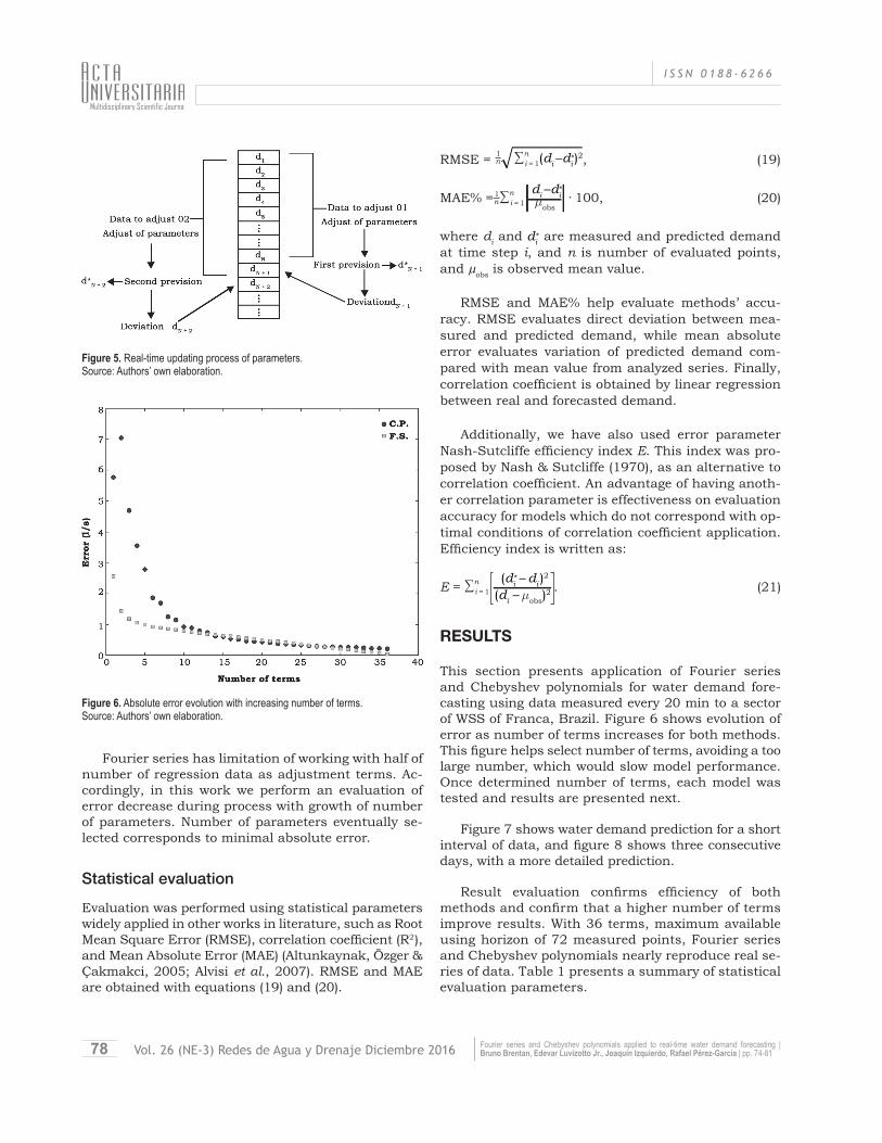
However, as in any extrapolation process, predic-tion error increases as forecasted value is far from used point values. Therefore, to reduce this error, ad-justable coefficients are updated at each time step, using water demand measured at last time and mov-ing window data forward. New window incorporates real value measured at time step N + 1 and allows a new calculation of adjustable coefficients. Figure 5 il-lustrates this updating process.

I S S N 0 1 8 8 - 6 2 6 6


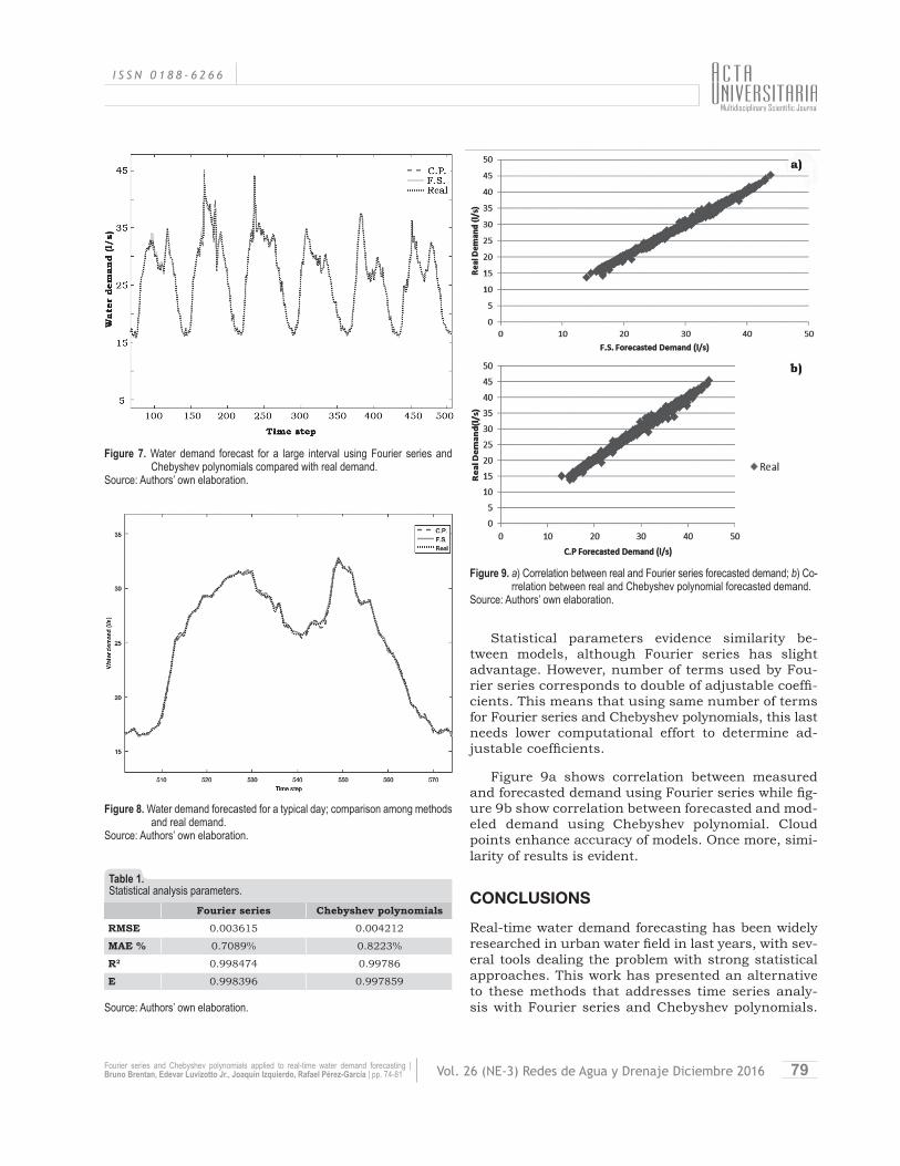
Fourier series has limitation of working with half of number of regression data as adjustment terms. Ac-cordingly, in this work we perform an evaluation of error decrease during process with growth of number of parameters. Number of parameters eventually se-lected corresponds to minimal absolute error.

Statistical evaluation Evaluation was performed using statistical parameters widely applied in other works in literature, such as Root Mean Square Error (RMSE), correlation coefficient (R2), and Mean Absolute Error (MAE) (Altunkaynak, Özger & Çakmakci, 2005; Alvisi et al., 2007). RMSE and MAE are obtained with equations (19) and (20).

RMSE = 1n ∑n

i = 1(di –di )2* , (19)

MAE% = ∑ni = 1

1n

di –di*

μobs· 100, (20)

where di and di* are measured and predicted demand

at time step i, and n is number of evaluated points, and μobs is observed mean value.

RMSE and MAE% help evaluate methods’ accu-racy. RMSE evaluates direct deviation between mea-sured and predicted demand, while mean absolute error evaluates variation of predicted demand com-pared with mean value from analyzed series. Finally, correlation coefficient is obtained by linear regression between real and forecasted demand.

Additionally, we have also used error parameter Nash-Sutcliffe efficiency index E. This index was pro-posed by Nash & Sutcliffe (1970), as an alternative to correlation coefficient. An advantage of having anoth-er correlation parameter is effectiveness on evaluation accuracy for models which do not correspond with op-timal conditions of correlation coefficient application. Efficiency index is written as:

E = ∑ni = 1

(di – di )2*

(di – μobs)2 . (21)

RESULTS

This section presents application of Fourier series and Chebyshev polynomials for water demand fore-casting using data measured every 20 min to a sector of WSS of Franca, Brazil. Figure 6 shows evolution of error as number of terms increases for both methods. This figure helps select number of terms, avoiding a too large number, which would slow model performance. Once determined number of terms, each model was tested and results are presented next.

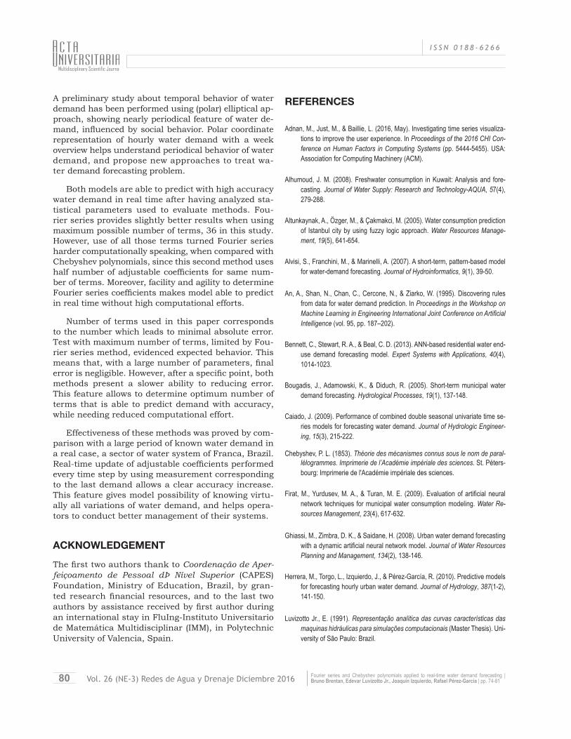
Figure 7 shows water demand prediction for a short interval of data, and figure 8 shows three consecutive days, with a more detailed prediction.

Result evaluation confirms efficiency of both methods and confirm that a higher number of terms improve results. With 36 terms, maximum available using horizon of 72 measured points, Fourier series and Chebyshev polynomials nearly reproduce real se-ries of data. Table 1 presents a summary of statistical evaluation parameters.

Figure 5. Real-time updating process of parameters.Source: Authors’ own elaboration.

Figure 6. Absolute error evolution with increasing number of terms.Source: Authors’ own elaboration.


I S S N 0 1 8 8 - 6 2 6 6


Statistical parameters evidence similarity be-tween models, although Fourier series has slight advantage. However, number of terms used by Fou-rier series corresponds to double of adjustable coeffi-cients. This means that using same number of terms for Fourier series and Chebyshev polynomials, this last needs lower computational effort to determine ad-justable coefficients.

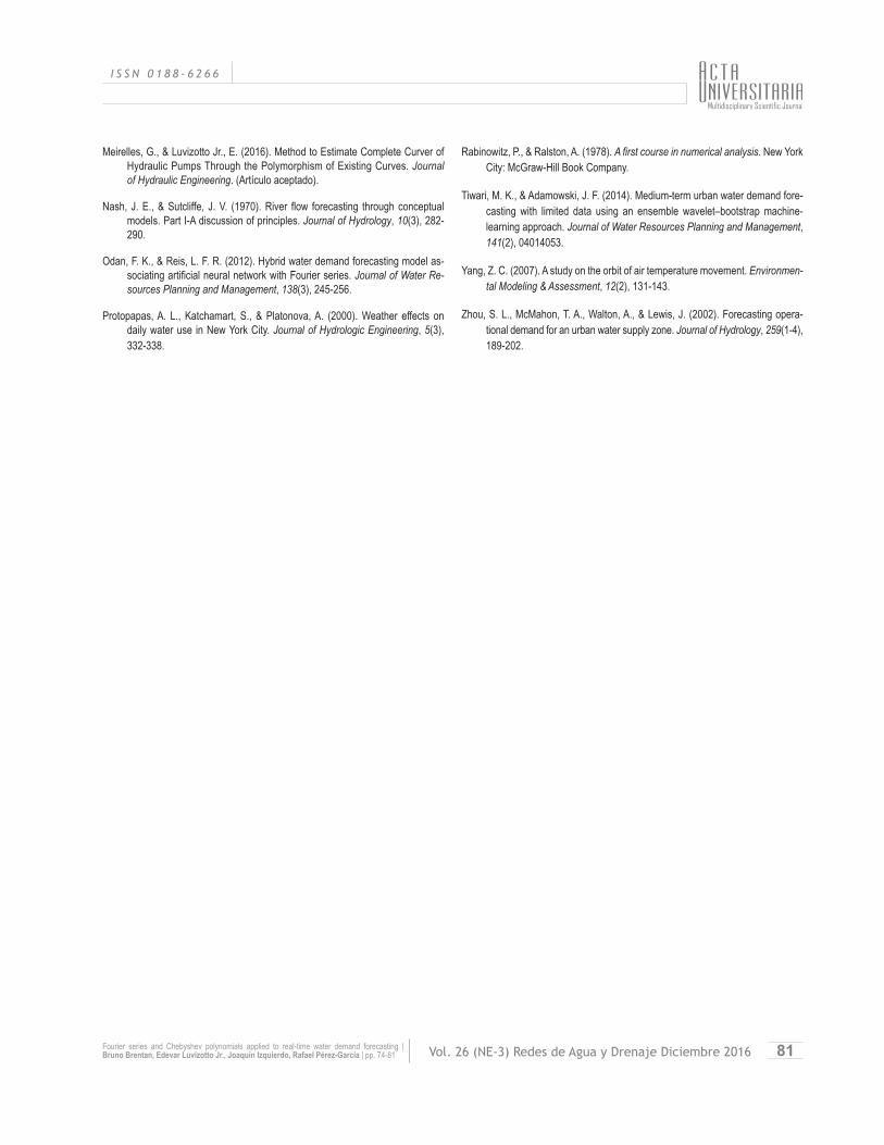
Figure 9a shows correlation between measured and forecasted demand using Fourier series while fig-ure 9b show correlation between forecasted and mod-eled demand using Chebyshev polynomial. Cloud points enhance accuracy of models. Once more, simi-larity of results is evident.

CONCLUSIONSReal-time water demand forecasting has been widely researched in urban water field in last years, with sev-eral tools dealing the problem with strong statistical approaches. This work has presented an alternative to these methods that addresses time series analy-sis with Fourier series and Chebyshev polynomials.

Figure 7. Water demand forecast for a large interval using Fourier series and Chebyshev polynomials compared with real demand.


Figure 9. a) Correlation between real and Fourier series forecasted demand; b) Co-rrelation between real and Chebyshev polynomial forecasted demand.


Figure 8. Water demand forecasted for a typical day; comparison among methods and real demand.


Fourier series Chebyshev polynomials

RMSE 0.003615 0.004212

MAE % 0.7089% 0.8223%

R2 0.998474 0.99786

E 0.998396 0.997859

Table 1. Statistical analysis parameters.


I S S N 0 1 8 8 - 6 2 6 6


A preliminary study about temporal behavior of water demand has been performed using (polar) elliptical ap-proach, showing nearly periodical feature of water de-mand, influenced by social behavior. Polar coordinate representation of hourly water demand with a week overview helps understand periodical behavior of water demand, and propose new approaches to treat wa-ter demand forecasting problem.

Both models are able to predict with high accuracy water demand in real time after having analyzed sta-tistical parameters used to evaluate methods. Fou-rier series provides slightly better results when using maximum possible number of terms, 36 in this study. However, use of all those terms turned Fourier series harder computationally speaking, when compared with Chebyshev polynomials, since this second method uses half number of adjustable coefficients for same num-ber of terms. Moreover, facility and agility to determine Fourier series coefficients makes model able to predict in real time without high computational efforts.

Number of terms used in this paper corresponds to the number which leads to minimal absolute error. Test with maximum number of terms, limited by Fou-rier series method, evidenced expected behavior. This means that, with a large number of parameters, final error is negligible. However, after a specific point, both methods present a slower ability to reducing error. This feature allows to determine optimum number of terms that is able to predict demand with accuracy, while needing reduced computational effort.

Effectiveness of these methods was proved by com-parison with a large period of known water demand in a real case, a sector of water system of Franca, Brazil. Real-time update of adjustable coefficients performed every time step by using measurement corresponding to the last demand allows a clear accuracy increase. This feature gives model possibility of knowing virtu-ally all variations of water demand, and helps opera-tors to conduct better management of their systems.

ACKNOWLEDGEMENT

The first two authors thank to Coordenação de Aper-feiçoamento de Pessoal dÞ Nível Superior (CAPES) Foundation, Ministry of Education, Brazil, by gran-ted research financial resources, and to the last two authors by assistance received by first author during an international stay in FluIng-Instituto Universitario de Matemática Multidisciplinar (IMM), in Polytechnic University of Valencia, Spain.

REFERENCES

Adnan, M., Just, M., & Baillie, L. (2016, May). Investigating time series visualiza-tions to improve the user experience. In Proceedings of the 2016 CHI Con-ference on Human Factors in Computing Systems (pp. 5444-5455). USA: Association for Computing Machinery (ACM).

Alhumoud, J. M. (2008). Freshwater consumption in Kuwait: Analysis and fore-casting. Journal of Water Supply: Research and Technology-AQUA, 57(4), 279-288.

Altunkaynak, A., Özger, M., & Çakmakci, M. (2005). Water consumption prediction of Istanbul city by using fuzzy logic approach. Water Resources Manage-ment, 19(5), 641-654.

Alvisi, S., Franchini, M., & Marinelli, A. (2007). A short-term, pattern-based model for water-demand forecasting. Journal of Hydroinformatics, 9(1), 39-50.

An, A., Shan, N., Chan, C., Cercone, N., & Ziarko, W. (1995). Discovering rules from data for water demand prediction. In Proceedings in the Workshop on Machine Learning in Engineering International Joint Conference on Artificial Intelligence (vol. 95, pp. 187–202).

Bennett, C., Stewart, R. A., & Beal, C. D. (2013). ANN-based residential water end-use demand forecasting model. Expert Systems with Applications, 40(4), 1014-1023.

Bougadis, J., Adamowski, K., & Diduch, R. (2005). Short-term municipal water demand forecasting. Hydrological Processes, 19(1), 137-148.

Caiado, J. (2009). Performance of combined double seasonal univariate time se-ries models for forecasting water demand. Journal of Hydrologic Engineer-ing, 15(3), 215-222.

Chebyshev, P. L. (1853). Théorie des mécanismes connus sous le nom de paral-lélogrammes. Imprimerie de l’Académie impériale des sciences. St. Péters-bourg: Imprimerie de l'Académie impériale des sciences.

Firat, M., Yurdusev, M. A., & Turan, M. E. (2009). Evaluation of artificial neural network techniques for municipal water consumption modeling. Water Re-sources Management, 23(4), 617-632.

Ghiassi, M., Zimbra, D. K., & Saidane, H. (2008). Urban water demand forecasting with a dynamic artificial neural network model. Journal of Water Resources Planning and Management, 134(2), 138-146.

Herrera, M., Torgo, L., Izquierdo, J., & Pérez-García, R. (2010). Predictive models for forecasting hourly urban water demand. Journal of Hydrology, 387(1-2), 141-150.

Luvizotto Jr., E. (1991). Representação analítica das curvas características das maquinas hidráulicas para simulações computacionais (Master Thesis). Uni-versity of São Paulo: Brazil.


I S S N 0 1 8 8 - 6 2 6 6


Meirelles, G., & Luvizotto Jr., E. (2016). Method to Estimate Complete Curver of Hydraulic Pumps Through the Polymorphism of Existing Curves. Journal of Hydraulic Engineering. (Artículo aceptado).

Nash, J. E., & Sutcliffe, J. V. (1970). River flow forecasting through conceptual models. Part I-A discussion of principles. Journal of Hydrology, 10(3), 282-290.

Odan, F. K., & Reis, L. F. R. (2012). Hybrid water demand forecasting model as-sociating artificial neural network with Fourier series. Journal of Water Re-sources Planning and Management, 138(3), 245-256.

Protopapas, A. L., Katchamart, S., & Platonova, A. (2000). Weather effects on daily water use in New York City. Journal of Hydrologic Engineering, 5(3), 332-338.

Rabinowitz, P., & Ralston, A. (1978). A first course in numerical analysis. New York City: McGraw-Hill Book Company.

Tiwari, M. K., & Adamowski, J. F. (2014). Medium-term urban water demand fore-casting with limited data using an ensemble wavelet–bootstrap machine-learning approach. Journal of Water Resources Planning and Management, 141(2), 04014053.

Yang, Z. C. (2007). A study on the orbit of air temperature movement. Environmen-tal Modeling & Assessment, 12(2), 131-143.

Zhou, S. L., McMahon, T. A., Walton, A., & Lewis, J. (2002). Forecasting opera-tional demand for an urban water supply zone. Journal of Hydrology, 259(1-4), 189-202.

Documents

Fourier series and Chebyshev polynomials applied to real