General Statistics

Ch En 475Unit Operations

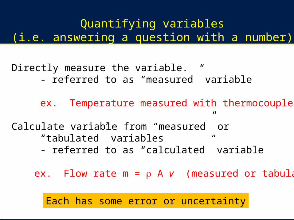
Quantifying variables(i.e. answering a question with a number)

1. Directly measure the variable. - referred to as “measured” variable

ex. Temperature measured with thermocouple

2. Calculate variable from “measured” or “tabulated” variables - referred to as “calculated” variable

ex. Flow rate m = r A v (measured or tabulated)

Each has some error or uncertainty

3

Outline

1. Error of Measured Variables2. Comparing Averages of Measured Variables

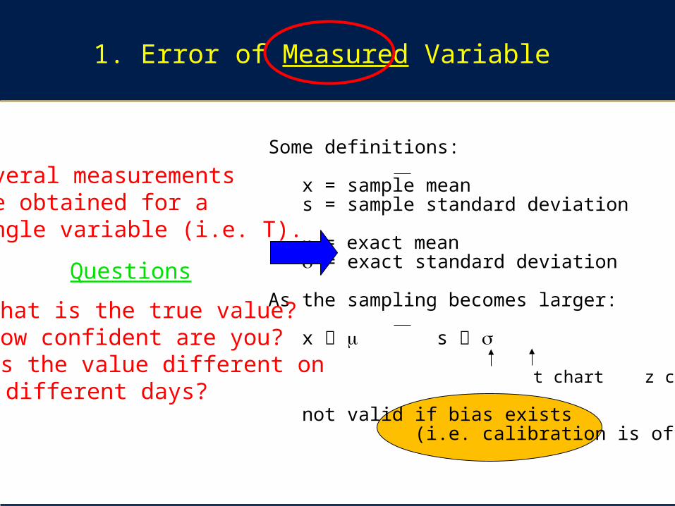
Some definitions:

x = sample means = sample standard deviation

m = exact means = exact standard deviation

As the sampling becomes larger:

x m s s

t chart z chart

not valid if bias exists (i.e. calibration is off)

1. Error of Measured Variable

Several measurementsare obtained for a single variable (i.e. T).

• What is the true value?• How confident are you?• Is the value different on different days?

Questions

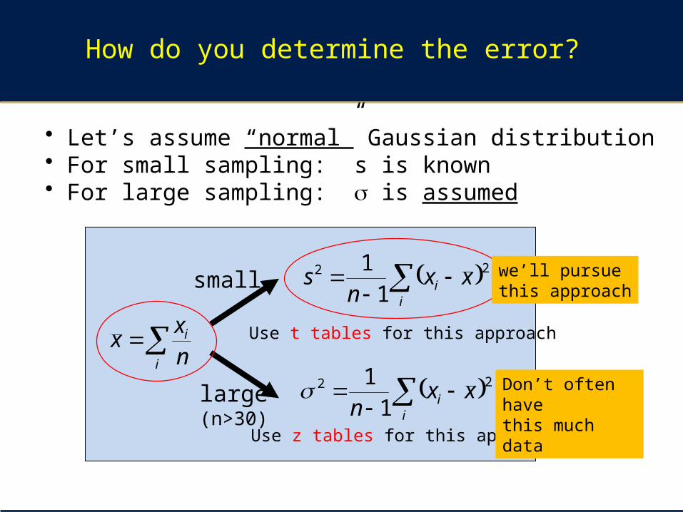
• Let’s assume “normal” Gaussian distribution • For small sampling: s is known• For large sampling: s is assumed

How do you determine the error?

i

i

nx

x

small

large(n>30)

i

i xxn

s 22

11

i

i xxn

22

11

we’ll pursue this approach

Use z tables for this approach

Use t tables for this approach

Don’t often have this much data

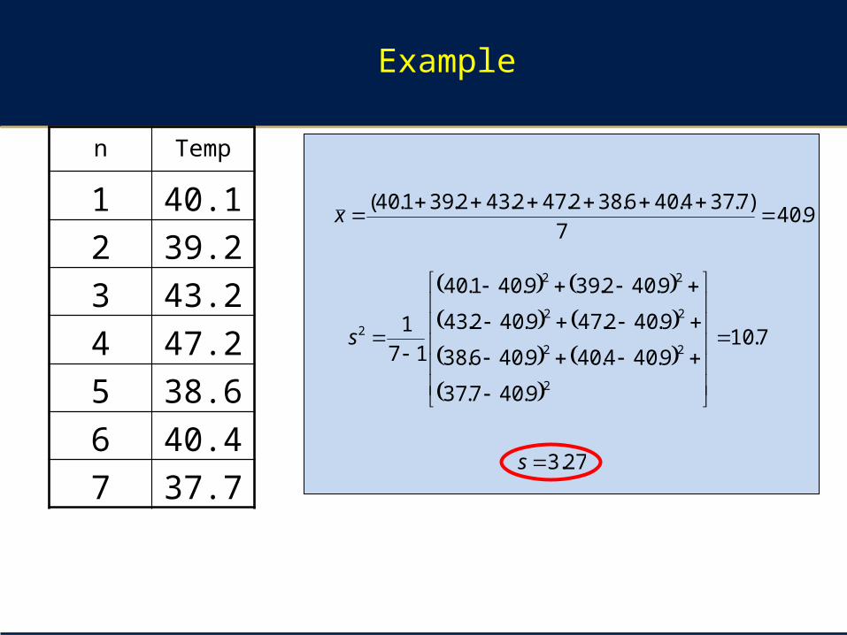
Example

n Temp

1 40.1

2 39.2

3 43.2

4 47.2

5 38.6

6 40.4

7 37.7

9.407

)7.374.406.382.472.432.391.40( x

7.10

9.407.37

9.404.409.406.38

9.402.479.402.43

9.402.399.401.40

17

1

2

22

22

22

2

s

27.3s

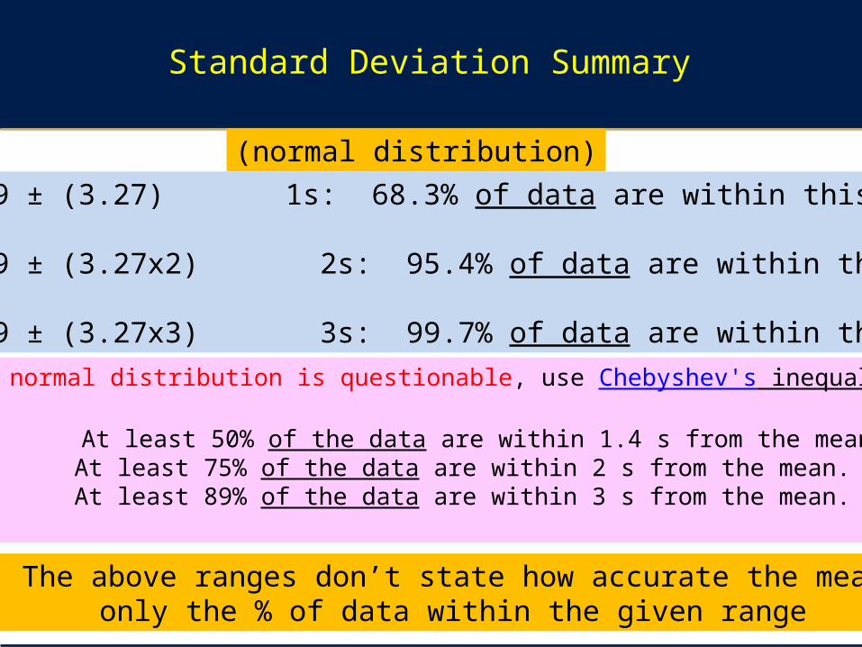
Standard Deviation Summary

(normal distribution)

40.9 ± (3.27) 1s: 68.3% of data are within this range

40.9 ± (3.27x2) 2s: 95.4% of data are within this range 40.9 ± (3.27x3) 3s: 99.7% of data are within this range

If normal distribution is questionable, use Chebyshev's inequality:

At least 50% of the data are within 1.4 s from the mean. At least 75% of the data are within 2 s from the mean. At least 89% of the data are within 3 s from the mean.

Note: The above ranges don’t state how accurate the mean is - only the % of data within the given range

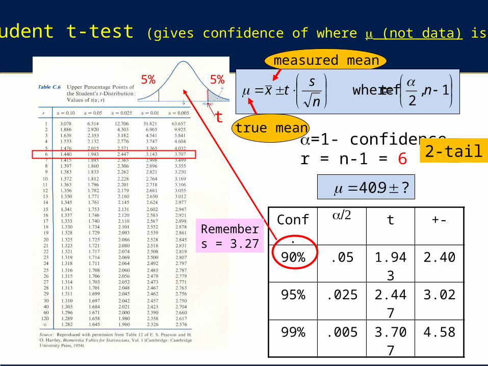
Student t-test (gives confidence of where m (not data) is located)

1,2

f t where nn

stx

a=1- confidencer = n-1 = 6

Conf. /2a t +-

90% .05 1.943 2.40

95% .025 2.447 3.02

99% .005 3.707 4.58

?9.40

5% 5%

ttrue mean

measured mean

2-tail

Remembers = 3.27

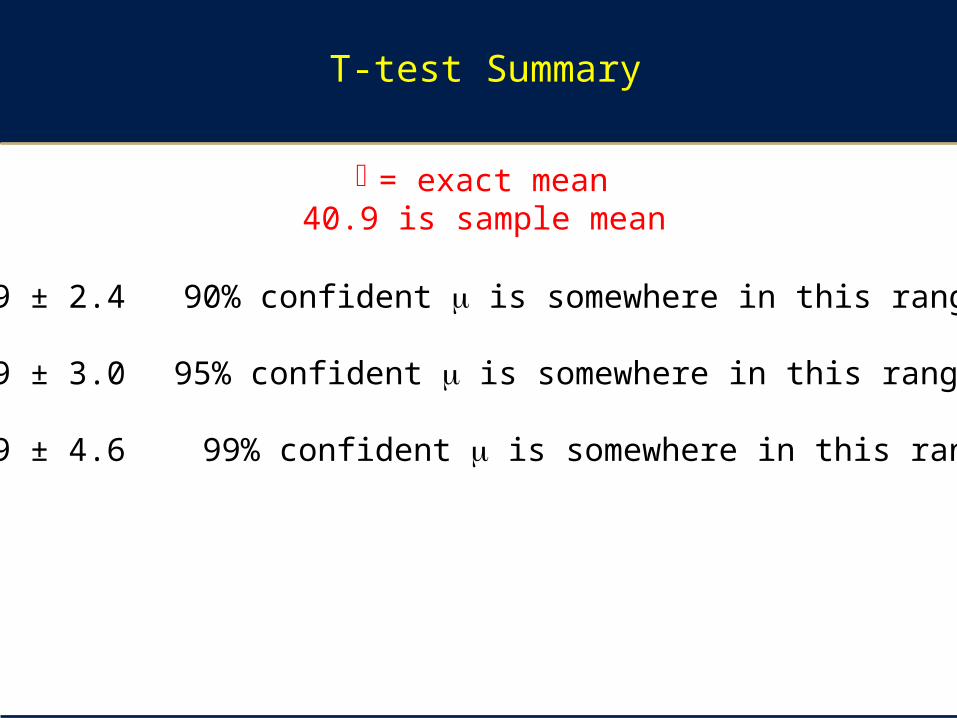
T-test Summary

40.9 ± 2.4 90% confident m is somewhere in this range

40.9 ± 3.0 95% confident m is somewhere in this range 40.9 ± 4.6 99% confident m is somewhere in this range

m= exact mean40.9 is sample mean

10

Outline

1. Error of Measured Variables2. Comparing Averages of Measured Variables

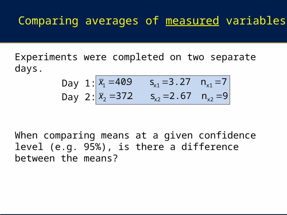
Experiments were completed on two separate days.

When comparing means at a given confidence level (e.g. 95%), is there a difference between the means?

Comparing averages of measured variables

Day 1:

Day 2: 9n 2.67 s 2.37

7n 3.27s 9.40

x2x22

x1x11

x

x

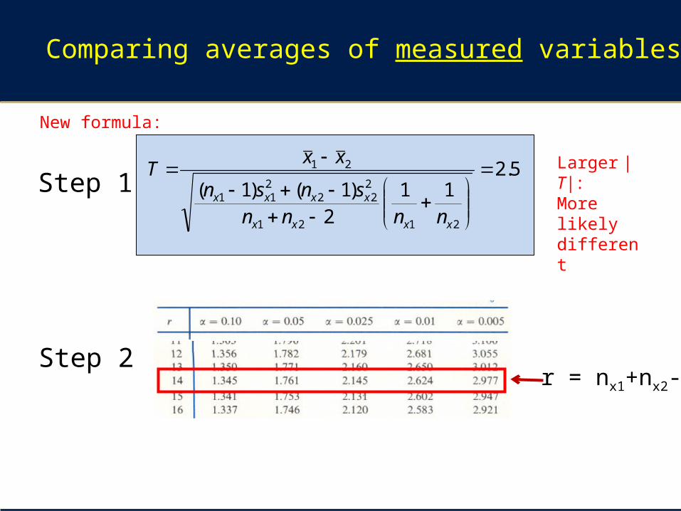
Comparing averages of measured variables

5.211

2

)1()1(

2121

222

211

21

xxxx

xxxx

nnnn

snsn

xxT

r = nx1+nx2-2

Larger |T|:More likelydifferent

Step 1

Step 2

New formula:

Comparing averages of measured variables

2-tail

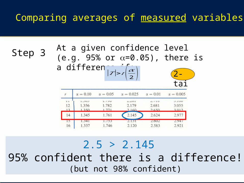
At a given confidence level (e.g. 95% or a=0.05), there is a difference if:

2.5 > 2.145 95% confident there is a difference!

(but not 98% confident)

Step 3

|𝑇|>𝑡 (𝛼2 )

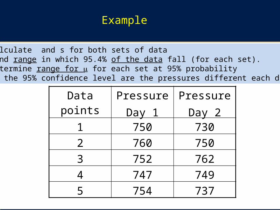
Example

1. Calculate and s for both sets of data2. Find range in which 95.4% of the data fall (for each set).3. Determine range for m for each set at 95% probability4. At the 95% confidence level are the pressures different each day?

Data points

PressureDay 1

PressureDay 2

1 750 730

2 760 750

3 752 762

4 747 749

5 754 737