Embed Size (px)
Citation preview
Nordic Hydrolgy, 26, 1995, 125- 146 No pd11 m,ty ix ~rprodured by .my proce\\ w~thout complete leference
Frost Heave due to Ice Lens Formation in Freezing Soils
1. Theory and Verification
D. Sheng, K. Axelsson and S. Knutsson Department of Civil Engineering,
Lulei University of Technology, Sweden
A frost heave model which simulates formation of ice lenses is developed for saturated salt-free soils. Quasi-steady state heat and mass flow is considered. Special attention is paid to the transmitted zone, i.e. the frozen fringe. The permeability of the frozen fringe is assumed to vary exponentially as a function of temperature. The rates of water flow in the frozen fringe and in the unfrozen soil are assumed to be constant in space but vary with time. The pore water pres- sure in the frozen fringe is integrated from the Darcy law. The ice pressure in the frozen fringe is detcrmined by the generalized Clapeyron equation. A new ice lens is assumed to form in the liozen fringe when and where the effective stress approaches zero. The neutral stress is determined as a simple function of the un- frozen water content and porosity. The model is implemented on an personal computer. The simulated heave amounts and heaving rates are compared with expcrimental data, which shows that the model generally gives reasonable esti- mation.
Introduction
The phenomenon of frost heave has been studied both experimentally and theoreti- cally for decades. Experimental observations suggest that frost heave is caused by ice lensing associated with thermally-induced water migration. Water migration can take place at temperatures below the freezing point, by flowing via the unfrozen wa- ter film adsorbed around soil particles. Overburden pressure, temperature gradient and depth to groundwater table are the most important factors that influence frost
D. Sheng, K. Axelsson and S. Knutsson
heave, Taber (1929, 1930), Penner and Ueda (1977), Penner (1986), Horiguchi (1987) and Konrad (1989).
Theoretically, a number of frost heave models have been proposed, e.g. Harlan (1 973), Konrad and Morgenstem (1 980, 198 1, 1982), Gilpin (1 980), Hopke (1 980), Guymon et al. (1 980, 1984), O'Neill and Miller (1980, 1985), Shen and Ladanyi (1987) and Padilla and Villeneuve (1992). These models are in general based upon the fundamental principles of thermodynamics and on experimental observations, and have been demonstrated very useful in understanding the phenomenon of frost heave and to some extent also in predicting frost heave for engineering purposes. In respect of
- Adequacy in describing the phenomenon, - Validation against e.g. experimental data, - Ease in determining input parameters, and - Applicability in solving practical problems
each of existing models has advantages and disadvantages and very few of them are satisfactory in all the aspects. For instance, the model by O'Neill and Miller (1985) has been considered to be physically elaborate in describing the phenomenon. How- ever, this model has not been validated by any experimental data. In addition, it is difficult to apply this model to solve practical problems which may involve e.g. stratified soil profiles, unsaturated soils, variable ground water table and capillarity, because some parameters needed are rarely available and difficult to determine. On the other hand, the models e.g. by Harlan (1973), Guymon et al. (1980, 1984) and Konrad and Morgenstem (1980, 198 1, 1982) deal with coupled heat and mass trans- fer in a scale of observation and have been applied to solve field problems. How- ever, an important feature of frost heave, i.e. the formation of discrete ice lenses, have not been considered in these models. Detailed review of the existing frost heave models may refer to O'Neill (1982), Berg (1984), Kay and Perfect (1988), Fu- kuda and Ishizaki (1 992) and Sheng (1 994).
In an effort to develop a frost heave model which takes into account the basic fea- tures of the phenomenon, but which excludes strange parameters, and more impor- tantly which can be further developed into an operational model for solving practical problems, Sheng et al. (1992) investigated a model which is somewhat a simplified version of that by Gilpin (1980). The soil was assumed to be saturated and salt-free. Quasi-steady state heat and mass flow was considered and the governing equations were established in a similar manner as by Gilpin (1980). It was assumed that ice lens initiation takes place when and where the maximum ice pressure reaches the to- tal overburden pressure plus the soil tensile strength. A linear variation in the perme- ability of the frozen fringe was also assumed. The input soil parameters were the dry density, the porosity, the saturated permeability and the thermal conductivity. The heave amounts computed were found very much dependent on the time step and the comparison with the experimental data was not satisfactory.
Frost Heave due to Ice Lens Formation in Freezing Soils I
In this paper, the investigated model will be modified so that a better computa- tional behaviour of the model and a better agreement between the model and experi- ments will be reached. Modifications are expected to be carried out in many aspects, e.g. in the expression of heat and mass equation, in the expression of the neutral stress, in what concerns the criterion for ice lens initiation, and in the permeability and unfrozen water content of the frozen fringe. The modified model will first be presented in this paper in a form of a research model, in order to gain an indepth understanding of the phenomenon, to justify various concepts used in the model and to simulate laboratory tests. In a following paper (this issue), it will be demonstrated that the research model can be further developed into an operational tool which can deal with field conditions such as a stratified soil profile, a varying ground water table, unsaturated soils and snow insulation on the ground surface.
Frozen Fringe and Ice Lens Formation
Freezing of a moist soil is essentially a process coupling heat and mass transfer. When a saturated fine-grained soil is subjected to a subfreezing temperature, part of the water in the soil pores can solidify into ice, i.e. pore ice particles; close to soil particles and more tightly bound to them, a film of unfrozen water remains. Accord- ing to thermodynamics, this adsorbed water film has lower free energy at a lower negative temperature. Therefore a potential gradient can develop along the tempera- ture gradient. Water can be sucked from the warm portion to replace the amount of water lost due to freezing and to feed the accumulation of pore ice. As the pore ice particles grow, they can finally contact each other and form an ice lens, oriented per- pendicular to the direction of heat and water flow. In fact, significant frost heave ob- served in field or laboratory is attributed to ice segregation and ice lens formation as- sociated with water migration.
It is observed that there exists a frozen zone between the growing ice lens and the frost front where the warmest pore ice exists. This zone has been referred to as the frozen fringe, Miller (1977) and Loch and Kay (1978). Within this frozen fringe the temperature drops from the freezing point at the frost front to the segregational tem- perature at the warm side of the ice lens. In response to this temperature drop, the pore water pressure, unfrozen water content and permeability also decrease through the fringe. The water pressure at the warm side of the lens, which appears in suction, is affected by the segregational temperature and the overburden pressure. Konrad (1989) measured the segregational temperature and pore water pressure in absence of overburden pressure and found they are related to each other by the Clapeyron equation. Unfrozen water content and the permeability decay more or less exponen- tially with decreasing temperature, Anderson et al. (1973), Burt and Williams (1 976).
D. Sheng, K. Axelsson and S. Knutsson
profile at time t profile at time t+At
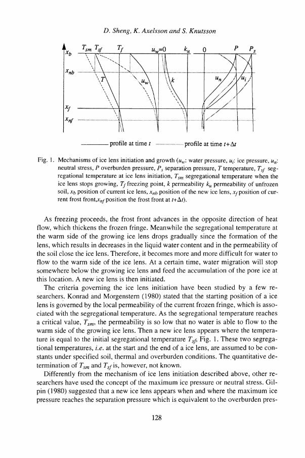
Fig. 1. Mechanisms of ice lens initiation and growth (u,,: water pressure, ui: ice pressure, u,,: neutral stress, P overburden pressure, P, separation pressure, T temperature, T,. seg- regational temperature at ice lens initiation, T,, segregational temperature when the ice lens stops growing, Tffreezing point, k permeability k , permeability of unfrozen soil, xh position of current ice lens, x,h position of the new ice lens, xfposition of cur- rent frost front,x,jposition the frost front at t+At).
As freezing proceeds, the frost front advances in the opposite direction of heat flow, which thickens the frozen fringe. Meanwhile the segregational temperature at the warm side of the growing ice lens drops gradually since the formation of the lens, which results in decreases in the liquid water content and in the permeability of the soil close the ice lens. Therefore, it becomes more and more difficult for water to flow to the warm side of the ice lens. At a certain time, water migration will stop somewhere below the growing ice lens and feed the accumulation of the pore ice at this location. A new ice lens is then initiated.
The criteria governing the ice lens initiation have been studied by a few re- searchers. Konrad and Morgenstem (1980) stated that the starting position of a ice lens is governed by the local permeability of the current frozen fringe, which is asso- ciated with the segregational temperature. As the segregational temperature reaches a critical value, Tsm, the permeability is so low that no water is able to flow to the warm side of the growing ice lens. Then a new ice lens appears where the tempera- ture is equal to the initial segregational temperature Tsfi Fig. 1 . These two segrega- tional temperatures, i.e. at the start and the end of a ice lens, are assumed to be con- stants under specified soil, thermal and overburden conditions. The quantitative de- termination of Tsm and Tsj is, however, not known.
Differently from the mechanism of ice lens initiation described above, other re- searchers have used the concept of the maximum ice pressure or neutral stress. Gil- pin (1 980) suggested that a new ice lens appears when and where the maximum ice pressure reaches the separation pressure which is equivalent to the overburden pres-
Frost Heave due to Ice Lens Formation in Freezing Soils I
sure plus the soil tensile strength, Fig. 1. In the model by O'Neill and Miller (1980), a neutral stress defined as the difference between the overburden pressure and the ef- fective stress is used instead of the ice pressure. A new ice lens appears when and where the maximum neutral stress reaches the overburden pressure, i.e. the effective stress vanishes. The generalized Clapeyron equation is used to relate the water pres- sure, ice pressure with the temperature within the frozen fringe. The neutral stress is equal to a weighted sum of water and ice pressure. The weight factor depends on the unfrozen water content and porosity. This criterion has advantage in quantitative ap- plication and will be employed in this paper. The weight factor in the expression of the neutral stress is, however, evaluated differently from O'Neill and Miller (1 985).
Frost Heave Model
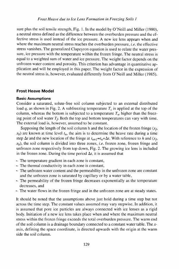
Basic Assumptions Consider a saturated, solute-free soil column subjected to an external distributed load q, as shown in Fig. 2. A subfreezing temperature T, is applied at the top of the column, whereas the bottom is subjected to a temperature T , higher than the freez- ing point of soil water Tf. Both the top and bottom temperatures can vary with time. The external load is, however, assumed to be constant.
Supposing the length of the soil column h and the location of the frozen fringe (x j xb) are known at time level t,, the aim is to determine the heave rate during a time step At and the new location of the fringe at t,+,=t,+At. With reference to h and (xj, xb), the soil column is divided into three zones, i.e. frozen zone, frozen fringe and unfrozen zone respectively from top down, Fig. 2. The growing ice lens is included in the frozen zone. During the time period At, it is assumed that
- The temperature gradient in each zone is constant, - The thermal conductivity in each zone is constant, - The unfrozen water content and the permeability in the unfrozen zone are constant
and the unfrozen zone is saturated by capillary or by a water table, - The permeability of the frozen fringe decreases exponentially as the temperature decreases, and
- The water flows in the frozen fringe and in the unfrozen zone are at steady states.
It should be noted that the assumptions above just hold during a time step but not across the time step. The constant values assumed may vary stepwise. In addition, it is assumed that pore ice particles are always connected with ice lenses as a rigid body. Initiation of a new ice lens takes place when and where the maximum neutral stress within the frozen fringe exceeds the total overburden pressure. The warm end of the soil column is a drainage boundary connected to a constant water table. The x- axis, defining the space coordinate, is directed upwards with the origin at the warm side the soil column.
D. Sheng, K. Axelsson and S. Knutsson
Fig. 2. Temperature, pore water pressure, permeability and unfrozen water content (W, un- frozen water content by volume).
The assumptions made above, which are expected to redace the number of parame- ters that are difficult to determine, will not violate the basic features of the phenom- enon of frost heave. For instance, the thermal conductivity is assumed to be constant in space but the permeability is assumed to vary across the frozen fringe. In reality, the both parameters change throughout the frozen fringe due to the change in unfro- zen water content. However the variation in the thermal conductivity is in general much less than in the permeability. This can be substantiated by experimental data e.g. by Black and Miller (1990) and Horiguchi and Miller (1983). According to Black and Miller (1990), if the unfrozen water content changes, for instance, from 0.5 to 0.25, the permeability will decrease from 10-8 to 5x10-11 d s , i.e. by a factor 0.005. The data by Horiguchi and Miller (1983) give similar correlations. The in- crease in thermal conductivity caused by the same change in the unfrozen water con- tent will, however, be less than 1.6 times, if the thermal conductivity is estimated by a geometric mean of the thermal conductivities of the soil phases. This change is small, compared to that in the permeability and therefore not considered in this mod- el.
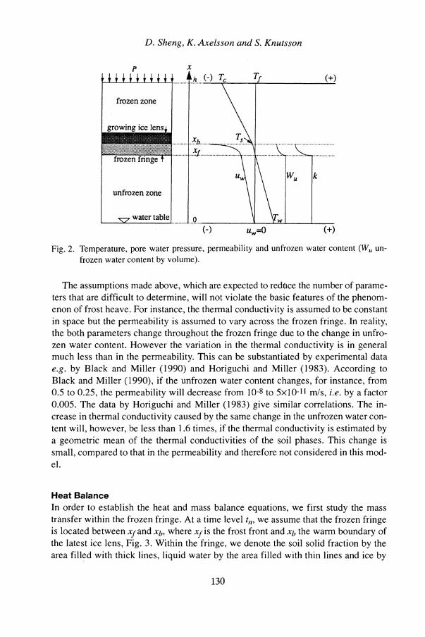
Heat Balance In order to establish the heat and mass balance equations, we first study the mass transfer within the frozen fringe. At a time level t,, we assume that the frozen fringe is located between xfand xb, where xfis the frost front and xb the warm boundary of the latest ice lens, Fig. 3. Within the fringe, we denote the soil solid fraction by the area filled with thick lines, liquid water by the area filled with thin lines and ice by
Frost Heave due to Ice Lens Formation in Freezing Soils 1
Existing ice at time level r,, Water Soil solid
0 New ice formed during At, to fill the space created due to rigid ice motion
New ice formed during At, due to the penetration of frost front
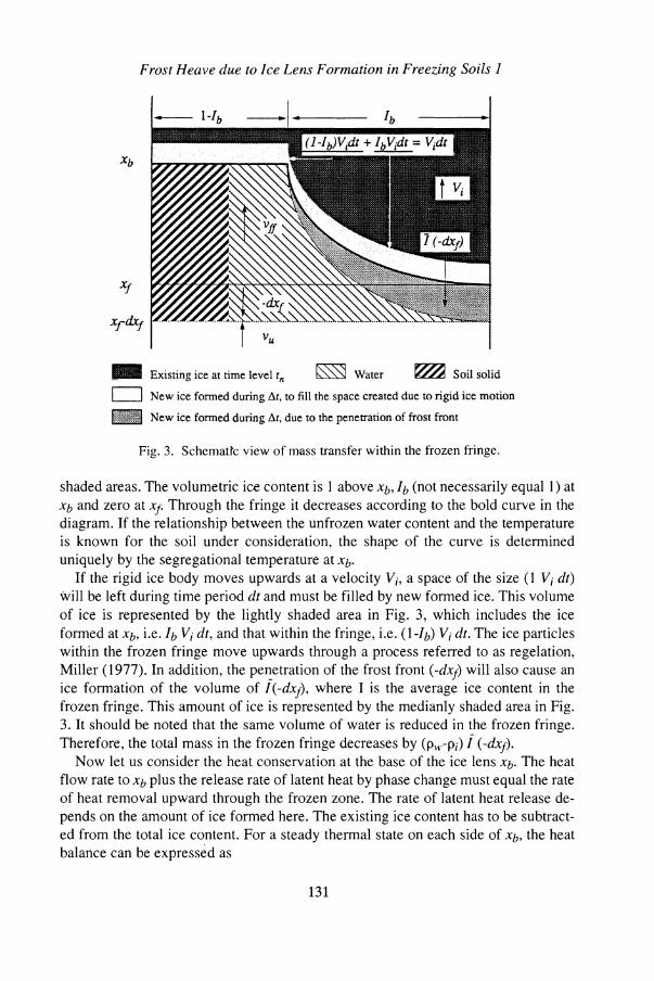
Fig. 3. Schematfc view of mass transfer within the frozen fringe.
shaded areas. The volumetric ice content is 1 above xb, Ib (not necessarily equal 1) at xb and zero at xf Through the fringe it decreases according to the bold curve in the diagram. If the relationship between the unfrozen water content and the temperature is known for the soil under consideration, the shape of the curve is determined uniquely by the segregational temperature at xb.
If the rigid ice body moves upwards at a velocity V;, a space of the size (1 V; dt) will be left during time period dt and must be filled by new formed ice. This volume of ice is represented by the lightly shaded area in Fig. 3, which includes the ice formed at xb, i.e. Ib Vi dt, and that within the fringe, i.e. (I-Ib) V; dt. The ice particles within the frozen fringe move upwards through a process referred to as regelation, Miller (1977). In addition, the penetration of the frost front (-dxf) will also cause an ice formation of the volume of i(-dxf), where I is the average ice content in the frozen fringe. This amount of ice is represented by the medianly shaded area in Fig. 3. It should be noted that the same volume of water is reduced in the frozen fringe. Therefore, the total mass in the frozen fringe decreases by @,-pi) (-dx$
Now let us consider the heat conservation at the base of the ice lens xb. The heat flow rate to xb plus the release rate of latent heat by phase change must equal the rate of heat removal upward through the frozen zone. The rate of latent heat release de- pends on the amount of ice formed here. The existing ice content has to be subtract- ed from the total ice content. For a steady thermal state on each side of xb, the heat balance can be expressed as
D. Sheng, K. Axelsson and S. Knutsson
where h is the height of the soil column, $and hfare the thermal conductivity of the frozen zone and frozen fringe respectively, L the specific latent heat of water, pi the density of ice, and Vi the rate of ice lens formation or the rate of heave.
Within the frozen fringe, the rate of ice formation is Vi due to rigid ice motion, in addition to (-dxf/d$ due to frost front penetration. Therefore, the overall heat bal- ance equation for the frozen fringe can be written as
where h, is the thermal conductivity of the unfrozen zone.
Pore Water Pressure and Mass Balance Since i t is assumed that the water flow rate in the frozen fringe, vg, is a constant, the pore water pressure can then be integrated from the Darcy law
where kfJ.is the permeability of the frozen fringe, p, the density of water and g the acceleration of gravity. The permeability kg is assumed to decrease exponentially through the frozen fringe
where k, is the permeability of unfrozen saturated soil and b a constant determined in a following section. Substituting Eq. (4) into Eq. (3) and integrating Eq. (3) from xf to x yields
where C is an integration constant and can be determined by substituting the boun- dary value of u, at xb. According to the generalized Clapeyron equation, this pore water pressure is related to the segregational temperature T, and the ice pressure at xb by, Kay and Groenevelt (1 974)
Frost Heave due to Ice Lens Formation in Freezing Soils I
where To is the freezing point of bulk water in degrees Kelvin, ui the ice pressure which equals the total overburden pressure. Eliminating the constant C from Eq. ( 5 ) by substituting Eq. ( 6 ) into Eq. ( 5 ) leads to
where p, is the geometric mean density of frozen soil interlayered with ice lenses. The mass conservation at xb requires that the water mass flowing to xb equals the
ice mass formed there
The overall mass balance within the frozen fringe states that the outflow of ice mass at xb equals the inflow of water mass at xf plus the decease of mass in the fringe
V . P . = v p + ( p - p . ) I ( - Z Z U W W Z xf (,C 5% (9)
The water flow rate in the unfrozen soil, v,, can be expressed by the Darcy law
The heat Eqs. (1) and (2), the pore water pressure Eq. ( 7 ) and the mass Eqs. (8) , ( 9 ) and (10) form the basis of the frost heave model. Providing the length of the soil column h and the initial location of the frozen fringe (xfi xb) are known, the six equations can be solved for the six unknowns T,, Vi, dxfidt, v#, v, and u,.(x). The equation system is non-linear because parameters such as Ib and b are dependent on the temperature T,. Therefore iteration is needed to solve the system.
Location of the Frozen Fringe The expression for the neutral stress or the effective pore pressure is proposed by Bishop (1 961) for ice-free unsaturated soil. Miller ( 1 977) used the same formula for air-free freezing soil
where x is a stress partitioning factor and is only a function of the degree of pore sat- uration, Snyder and Miller (1985). Miller ( 1 977) first approximated x by w,ln, i.e. the fraction of unfrozen water with respect to the pore space. Hopke (1980) tested
D. Sheng, K. Axelsson and S. Knutsson
this approximation but found cyclic increases and decreases in the heaving rate. This cyclic behavior of heaving rate was considered unreasonable by Hopke ( 1 980) but observed late by Penner (1986). In O'Neill and Miller's Model, x was initially set to (w,ln)1.5 (O'Neill and Miller 1980) and then upgraded to an equivalent expression by Snyder and Miller (1985). However, the two different expressions for x did not lead to any apparent difference in the computed results if we compare the two papers by O'Neill and Miller (1980, 1985), though the authors did not mention this differ- ence. Therefore, we use the simple expression by Miller (1 977) for the parameter X , which results in
I a = an + Ou +- u . = a n w n z +un
where a denotes the total overburden pressure, o' the effective stress, u, the neutral stress, n the soil porosity and I the ice content.
Providing the maximum neutral stress in the frozen fringe governs the initiation of a new ice lens, the aim is to search for the position where the maximum value oc- curs. Substituting the Clapeyron Eq. (6) to replace the ice pressure ui in Eq. (12) yields
Again Eq. ( 1 3) is non-linear because of the temperature-dependent ice content I. The derivative du,ldx is a very complex function of x and the solution dunldx=O can not be found easily. In order to find the position of the maximum neutral stress, xnb, we divide the frozen fringe (xf; xb) into m equal intervals and compute u, at each divid- ing point. The maximum neutral stress and its position can then be determined by interpolation. This maximum value of neutral stress is then compared with the total overburden pressure. If the overburden pressure is exceeded, a new ice lens is as- sumed to appear at the position x,b. The new frozen fringe is located between xb, and xf: Otherwise, no new ice lens appears and the position xb remains during next time step.
So far, the frost heave model is established based upon the knowledge of the ini- tial location of the frozen fringe. The depth of frost penetration during the first time step can be computed approximately by e.g. the Neumann solution for pure phase change problems. By assuming an initial segregational temperature, the location of the first ice lens can be determined by interpolation. The initial segregational tem- perature can be modified after the system of the heat and mass equations have been solved. The location of the first frozen fringe can then be determined by iteration.
Equilibrium Situation The previous discussion is based on the existence of the frozen fringe. In the case the rate of frost penetration -dxfldt is slower than the moving rate of the cold boundary
Frost Heave due to Ice Lens Formation in Freezing Soils I
of the frozen fringe xb, the frozen fringe will become thinner and thinner, Once the distance between xb and xf is too small for computation significance, the frozen fringe is expected to disappear. This is the case when the frost front penetrates close enough to the warm boundary of the soil column. The water flow rate in the unfro- zen zone is then in equilibrium with the rate of ice lens formation and thus the frost front will stay still. The heat balance equation becomes
The Clapeyron Eq. (6 ) can still be used to determine the pore water pressure at the frost front. The mass balance at the frost front is simplified to
where v, is determined by (10). The four Eqs. (6) , ( l o ) , (14) and (15) can be solved for the four unknowns T,, Vi , u,(xb) and v,. The soil column is elongated by (-Vi)At after each time step.
Material Properties Theoretically all the parameters used in the frost heave model could be treated as in- put data. This, however, could limit the potential applicability of the model. In order to avoid parameters that are too elaborate to determine, we introduce some empirical relations.
The effective thermal conductivity in the unfrozen zone and the frozen fringe can be computed using the geometric mean
where the subscripts s, w and i respectively stand for the soil solid phase, the water phase and the ice phase. The mean value of the volumetric ice content equals zero in the unfrozen zone.
In the frozen zone, frozen soil is interlayered with pure ice lenses. The equivalent thermal conductivity can be calculated in a manner analogous to the resistance in a series electrical circuit, i.e.using a harmoic mean
where hf is the thermal conductivity of frozen soil and can be determined by Eq. (16) with I=n, and h, the initial height of the soil column.
The constant b in Eq. (4) can be determined by substituting the permeability at the base of the growing ice lens. The expression suggested by O'Neill and Miller (1985) can be used to calculate this permeability, which gives
D. Sheng, K. Axelsson and S. Knutsson
The volumetric unfrozen water content W , in the frozen fringe can be expressed as a function of the local temperature or a function of the pore pressure difference (u,- u;), Anderson and Tice (1973), O'Neill and Miller (1985), Kujala (1989) and Black and Miller (1 990). Alternative relationships have been obtained by regression of ex- perimental data. For instance, that by Black and Miller (1 990) states
where +;,. the pressure difference between water and ice. This equation can of course be applied in our model. In fact, by using the Clapeyron equation this for- mula can also be expressed in terms of temperature. However, the parameters in the formula are not easy to determine and limited experimental data are available.
Another relationship is given by Kujala (1 989, 199 1)
a (9) 0
n -I = W (T) = Wo e U
where Wo is the initial volumetric water content and ci and parameters dependent on soil specific surface area and pore geometry. This formula is obtained based on 126 laboratory measurements of totally 68 samples covering both coarse and fine finish soils. The parameter @ approximately equals 2 for most soils of interest. The parameter ci can be determined by substituting the unfrozen water content at a sub- freezing temperature e.g. -1.0 OC. In the model discussed here, Eq. (19) is applied with P=2.
Computation Strategy Now we summarize the frost heave model described above. Knowing the following conditions at t=O
- Initial height of soil column, - Soil porosity and dry density, - Thermal conductivity of soil solid particles, - Permeability of unfrozen saturated soil, - Unfrozen water content at a subfreezing temperature, e.g. -1 OC, - Overburden pressure and initial and boundary temperatures.
We first determine the position the first ice lens according to the theory discussed in the section location of the frozen fringe. The heat and mass balance Eqs. (1) and (2) and Eqs.(7)-(lo) are then solved by iteration, for the segregational temperature T,, the rate of ice lens formation V;, the rate frost front penetration dxf ldt, and the pore water pressure u,(x). The length of the soil column is elongated by V; At. The frost front moves (-dxfldt) At downwards. The position of the new frozen fringe is deter-
Frost Heave due to Ice Lens Formation in Freezing Soils I
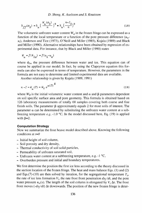
Justify Ice Lens Initiation - 1 * [ Relocate Moving Boundaries 1 1
L I
next time step Fig. 4. Flow chart of the frost heave model.
mined according to the ice lens formation criterion described by Eqs. (12)-(13). The system is then ready for next time step. This procedure is illustrated by Fig. 4.
A computer programme for the process described above has been developed and computer graphics has been used to represent heaved soil columns enclosing ice lenses, history diagrams of heave, of frost front, of segregational temperature and of suction in pore water pressure in the frozen fringe. The input parameters include dry density, porosity, saturated permeability, unfrozen water content at a subfreezing temperature, thermal conductivity, boundary temperatures, length of soil column, freezing time and time step for computation.
Experimental Verification
Experimental studies on frost heave have been carried out by many researchers. In this paper, the laboratory results presented by Takeda and Nakano (1990), Penner and Ueda (1 977), and Konrad and Morgenstem (1 980) are chosen to verify the mod- el presented. The tests by Penner and Ueda are representative for studying the effect of overburden pressures, whereas Konrad and Morgenstem for temperature gra- dients and Takeda and Nakano for soil types.
Although the test conditions and soil properties are described relatively in detail in these three references, some input parameters needed for simulation are not given. One of them is the unfrozen water content at a subfreezing temperature. If a series of tests on the same sample have been carried out, the parameters needed can be back- estimated using the results from one of the tests and then applied to simulate the oth- ers. Otherwise, average values for the soils are used.
Takeda and Nakano (1990) Freezing tests on three soil samples were conducted using a steady-state method in which the temperature profiles in the soil specimens were controlled. The three soil samples were Kanto loam, Tomakomai silt and Fujinomori clay, with the basic prop-
D. Sheng, K. Axelsson and S. Knutsson
Table 1 - Soil properties and test conditions of the tests by Takeda and Nakano
Soil sample Kanto loam Tomakomai silt Fujinomori clay
Dry density kgIm3 Porosity % Saturation degree % Specific surface area 10-3 m21kg Plasticity index % Permeability * 10-8 m/s Thermal conductivity WlmK Top temperatures "C Bottom temperature "C Unfrozenlinitial water content at -1 OC,%
* Calculated from the given hydraulic conductivity. i Best fit.
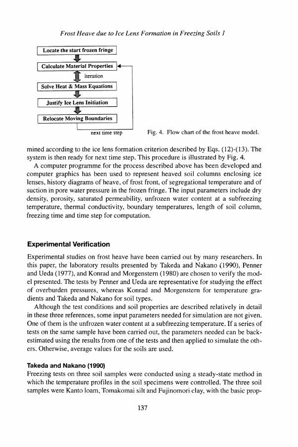
erties listed in Table 1. Two cylindrical soil specimens, 4 cm long and 2.8 cm in di- ameter, placed parallel to each other in the test cell, were thoroughly insulated so that they freezes unidirectionally from top down. The top and bottom temperatures were adjusted during the tests. No overburden pressure was applied during freezing. Heave and temperature as well as water intake rate were measured.
The simulation of the tests is carried out for a time period 55 hours, with a time step equal to 19.8 seconds. The unfrozen water content at - 1 O C is determined so that the measured heave is best fitted. The best fitted value of unfrozen water content is then adjusted with reference to the given specific surface areas. The boundary tem- peratures used in the simulation are not exactly the same as those in the tests, but the average cooling or heating rate is used.
The computed and measured values of heave are plotted versus time in Fig. 5, which shows that a general agreement between the simulated and measured heave exists. It is observed that the model slightly underestimates frost heave for the Kan- to loam and the Tomakomai silt, but matches well for the Fujinomori clay.
0 10 20 30 40 50 60 Time (hours)
r Tomakomai silt Fujinomori clay Kanto loam ------. Tomakomai silt
lines: simulated points: measured
Fig. 5. Computed and measured heave for tests by Takeda and Nakano.
the
Frost Heave due to Ice Lens Formation in Freezing Soils 1
Table 2 - Soil properties and test conditions of tests by Penner and Ueda
Soil sample No. 2 No. 4 No. 5 No. 9
Initial water cont. by dry weight Yo 16.3 19.5 Dry density kg/m3 1870 1780 Porosity 0.35 0.35 Permeability* 10-8 rnls 1 .0 0.5 Ther. conduc. of soil solid* WlmK 3.0 3.0 Average top temperature "C -1.45 -1.75 Average bottom temperature "C 2.4 1.9 Unfrozenlinitial water content t at -1.0 OC % 36 4 1
* Average values. t Best fit of the measured heave under the lowest overburden pressure.
Table 3 - Computed and measured heave rates for the tests by Penner and Ueda
Pressure Initial length Total heave rate, crnlhour Computed soil sample kPa cm measured computed Measured
No. 2 49.0 10.87 1 .67~10-2 *1.67xlO-2 I .00 98.1 10.66 1.45x10⁻² 1 .33~1 10-2 0.92
294.2 10.64 0.42 x 10⁻² 0.61 x 10⁻² 1.45 490.3 10.87 0.1 1 x 10⁻² 0.32 x 10⁻² 2.91
No. 4 49.0 9.86 2.28 x 10-2 *2.29 x 10-2 1 .OO 147.1 9.4 1 .08~10-2 1 .63~10-2 1.5 1 245.2 9.76 0.5 1 x 10⁻² 0.7 1 x 10⁻² 1.40 343.2 9.88 0.27 x 10⁻² 0.80 x 10⁻² 2.96
No. 5 98.1 9.73 1 . 0 1 ~ 1 0 - 2 *1.01x10-2 1 .00 196.1 9.97 0.49 x 10⁻² 0.67 x 10⁻² 1.37 392.3 9.64 0.26 x 10⁻² 0.28 x 10⁻² 1.08 490.3 9.43 0 . 1 0 ~ 10-2 0 . 1 0 ~ 10-2 1 .00
No. 9 49.0 9.82 3.15 x 10⁻² "3.15 x 10⁻² 1 .00 147.1 10.15 2.25 x 10⁻² 2.28 x 10⁻² 1.02 245.2 10.07 1 . 5 9 ~ 10-2 1 . 6 0 ~ 10-2 1.01 343.2 9.96 0.90xl0-2 1 .13~10-2 1.26
* Best fit by adjusting the unfrozen water content at -I .0 "C.
Penner and Ueda (1977) Heaving rates under various overburden pressures were measured in unidirectional freezing tests with constant boundary temperatures. The soils studied include a silty sand i.e. No. 2, two silts i.e. No. 4 and No. 5 , and clayey silt i.e. No. 9. The soil sam- ples are all saturated. The physical properties are listed in Table 2. The unfrozen wa- ter content at - 1 O C , in percentage of the initial water content, is back-estimated from
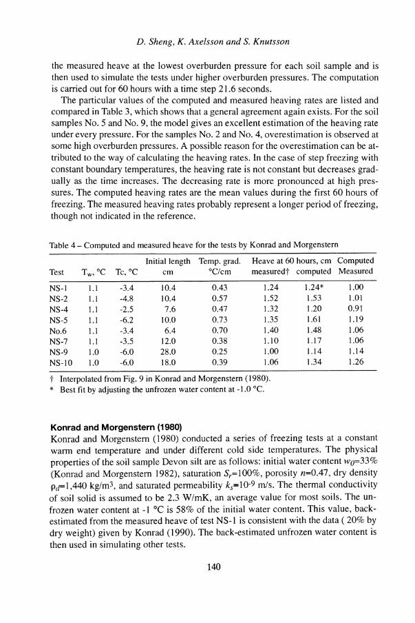
D. Sheng, K. Axelsson and S. Knutsson
the measured heave at the lowest overburden pressure for each soil sample and is then used to simulate the tests under higher overburden pressures. The computation is carried out for 60 hours with a time step 21.6 seconds.
The particular values of the computed and measured heaving rates are listed and compared in Table 3, which shows that a general agreement again exists. For the soil samples No. 5 and No. 9, the model gives an excellent estimation of the heaving rate under every pressure. For the samples No. 2 and No. 4, overestimation is observed at some high overburden pressures. A possible reason for the overestimation can be at- tributed to the way of calculating the heaving rates. In the case of step freezing with constant boundary temperatures, the heaving rate is not constant but decreases grad- ually as the time increases. The decreasing rate is more pronounced at high pres- sures. The computed heaving rates are the mean values during the first 60 hours of freezing. The measured heaving rates probably represent a longer period of freezing, though not indicated in the reference.
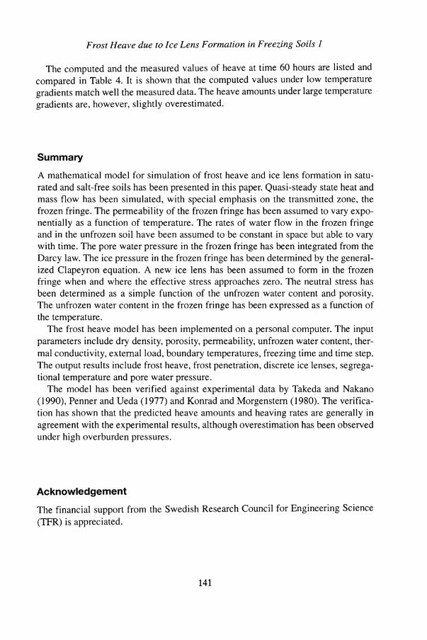
Table 4 - Computed and measured heave for the tests by Konrad and Morgenstern
Initial length Temp. grad. Heave at 60 hours, cm Computed Test T,, "C Tc, "C cm "Cicm measured? computed Measured
NS-I 1.1 -3.4 10.4 0.43 1.24 1.24* 1 .00 NS-2 1.1 -4.8 10.4 0.57 1.52 1.53 I .O1 NS-4 1 . I -2.5 7.6 0.47 1.32 1.20 0.91 NS-5 1.1 -6.2 10.0 0.73 1.35 1.61 1.19 No.6 1.1 -3.4 6.4 0.70 1.40 1.48 1.06 NS-7 1 . I -3.5 12.0 0.38 1.10 1.17 1.06 NS-9 1.0 -6.0 28.0 0.25 1 .OO 1.14 1.14 NS-I0 1.0 -6.0 18.0 0.39 1.06 1.34 1.26
Interpolated from Fig. 9 in Konrad and Morgenstern (1980). * Best fit by adjusting the unfrozen water content at -1.0 "C.
Konrad and Morgenstern (1980) Konrad and Morgenstern (1980) conducted a series of freezing tests at a constant warm end temperature and under different cold side temperatures. The physical properties of the soil sample Devon silt are as follows: initial water content wo=33% (Konrad and Morgenstern 1982), saturation S,.=100%, porosity n=0.47, dry density ppl ,440 kglm3, and saturated permeability ks=lO-9 mls. The thermal conductivity of soil solid is assumed to be 2.3 WImK, an average value for most soils. The un- frozen water content at -1 "C is 58% of the initial water content. This value, back- estimated from the measured heave of test NS-I is consistent with the data ( 20% by dry weight) given by Konrad (1990). The back-estimated unfrozen water content is then used in simulating other tests.
Frost Heave due to Ice Lens Formation in Freezing Soils I
The computed and the measured values of heave at time 60 hours are listed and compared in Table 4. It is shown that the computed values under low temperature gradients match well the measured data. The heave amounts under large temperature gradients are, however, slightly overestimated.
Summary
A mathematical model for simulation of frost heave and ice lens formation in satu- rated and salt-free soils has been presented in this paper. Quasi-steady state heat and mass flow has been simulated, with special emphasis on the transmitted zone, the frozen fringe. The permeability of the frozen fringe has been assumed to vary expo- nentially as a function of temperature. The rates of water flow in the frozen fringe and in the unfrozen soil have been assumed to be constant in space but able to vary with time. The pore water pressure in the frozen fringe has been integrated from the Darcy law. The ice pressure in the frozen fringe has been determined by the general- ized Clapeyron equation. A new ice lens has been assumed to form in the frozen fringe when and where the effective stress approaches zero. The neutral stress has been determined as a simple function of the unfrozen water content and porosity. The unfrozen water content in the frozen fringe has been expressed as a function of the temperature.
The frost heave model has been implemented on a personal computer. The input parameters include dry density, porosity, permeability, unfrozen water content, ther- mal conductivity, external load, boundary temperatures, freezing time and time step. The output results include frost heave, frost penetration, discrete ice lenses, segrega- tional temperature and pore water pressure.
The model has been verified against experimental data by Takeda and Nakano (1 990), Penner and Ueda (1 977) and Konrad and Morgenstern (1980). The verifica- tion has shown that the predicted heave amounts and heaving rates are generally in agreement with the experimental results, although overestimation has been observed under high overburden pressures.
Acknowledgement
The financial support from the Swedish Research Council for Engineering Science (TFR) is appreciated.
D. Sheng, K. Axelsson and S. Knutsson
Notations g Acceleration of gravity h Length of soil column I Ice content Ib Ice content at the base of the growing ice lens I Mean ice content in the frozen fringe k Permeability
kfJ Permeability of the frozen fringe k, Saturated permeability of unfrozen soil L Specific latent heat of water n Porosity of soil q Overburden pressure t Time At Time step T Temperature T,. Applied temperature at the cold side
Freezing temperature soil moisture To Freezing point of bulk water T, Segregational temperature
TSf Segregational temperature at the start of a ice lens T,, Segregational temperature at the end of a ice lens T, Applied temperature at the warm side U , Ice pressure u, Neutral stress u,, Pore water pressure
VB Rate of water flow in the frozen fringe v, Rate of water flow in the unfrozen soil V, Rate of ice lensing (rate of heave) W , Unfrozen water content by volume w, Unfrozen water content by dry weight xb Base position of the growing ice lens
XJ Position of frost front (0-isotherm) x,b Base position of the new ice lens
xnj Position of the new frost front
hj Thermal conductivity of frozen soil
Af Effective thermal conductivity of frozen soil with ice lenses
A# Thermal conductivity of frozen fringe A, Thermal conductivity of ice A, Thermal conductivity of soil solid A, Thermal conductivity of unfrozen soil A, Thermal conductivity of water p, Total density of frozen soil p , Density of ice p , Density of water cr' Effective stress x Stress partitioning factor
"C "C
degree Kelvin "C "C "C "C Pa Pa Pa
m/s m/s m/s
Frost Heave due to Ice Lens Formation in Freezing Soils 1
References
Anderson, D. M., and Tice, A. R. (1973) The unfrozen interfacial phase in frozen soil-water systems, Ecological Studies, Springer Verlag, Vol. 4, pp. 107-124.
Berg, R. L. (1 984) Status of numerical models for heat and mass transfer in frost-susceptible soils, 4 th Int. Conf. Permafrost, Final Proc., National Academy Press, Washington, D.C., pp. 67-7 1.
Black, P. B., and Miller, R. D. (1985) A continuum approach to modelling of frost heaving. In Freezing and Thawing of Soil-Water Systems (D. M. Anderson and P. J. Williams, eds.) Technical Council on Cold Regions Engineering Monograph, ASCE, pp. 36-43.
Black, P. B., and Miller, R. D. (1990) Hydraulic conductivity and unfrozen water content of air-free frozen silt, Water Resour. Res., Vol. 26, No. 2 , pp. 323-329.
Burt, T. P., and Williams, P. J. (1976) Hydraulic conductivity in frozen soils, Earth Surface Processes, Vol. I , pp. 349-360.
Eigenbrod, KD, Knutsson, S., and Sheng, D. (1991) Measurement of pore pressures in freez- ing and thawing soft fine-grained soils, Proc. of 44 th. Can. Geotech. Conf., Winnipeg, Canada Geotechnical Society.
Farouki, 0 . T. (1986) Thermal properties of soils, Clausthal-Zellerfeld, Trans Tech Publica- tion.
Fukuda, M., and Ishizaki, T. (1992) General report on heat and mass transfer, Proc. 6th Int. Symp. Ground Freezing, Balkema, otter dam, Vol. 2, pp. 409-416.
Gilpin, R. R. (1 980) A model for the prediction of ice lensing and frost heave in soils, Water Resour. Res., Vol. 16, No. 5 , pp. 918-930.
Groenevelt, P. H., and Kay, B. D. (1974) On the interaction of water and heat transport in fro- zen and unfrozen soils: i. basic theory; the liquid phase, Soil Sci. Soc. Amer. Proc., Vol. 38, pp. 400-404.
Guymon, G. L., Hromadka 11, T. V., and Berg, R. L. (1980) A one-dimensional frost heave model based upon simulation of simultaneous heat and water flux, Cold Reg. Sci. Technol., Vol. 3, pp. 253-262.
Guymon, G. L., Hromadka 11, T. V., and Berg, R. L. (1984) Two-dimensional model of cou- pled heat and moisture transport in frost-heaving soils, J. Energy Resour. Technol., Vol. 106, No. 3, pp. 336-343.
Harlan, R. L. (1973) Analysis of coupled heat and mass transfer in partial frozen soil, Water Resour. Res., Vol. 9 , No. 5 , pp. 13 14-1 323.
Holden, J. T., Piper, D., and Jones, R. H. (1985) Some development of a rigid-ice model of frost heave, Proc. 4th Int. Symp. Ground Freezing, Balkema, Rotterdam, pp. 93-98.
Hopke, S. (1980) A model for frost heave including overburden, Cold Reg. Sci. Technol., Vol. 3, pp. 111-127.
Horiguchi, K. (1 987) Effect of cooling rate on freezing of saturated soil, Cold Reg. Sci. Tech- nol., Vol. 14, pp. 147-153.
Horiguchi, K., and Miller, R. D. (1983) Hydraulic conductivity functions of frozen materials, Proc. 4th Int. Conf. Permafrost, National Academy Press, Washington, D.C., pp. 504-508.
Jame, Y. W., and Norum, D. I. (1980) Heat and mass transfer in a freezing unsaturated porous medium, Water Resour. Res., Vol. 16, pp. 8 11 -81 9.
Jansson, P.-E., and Halldin, S. (1979) Model for the annual water and energy flow in a layered soil, Comparison offrost and energy models (S. Halldin, ed), Soc. Ecol. Modelling, Copen-
D. Sheng, K. Axelsson and S. Knutsson
hagen, pp. 145-163. Kay, B. D., and Groencvelt, P. H. (1974) On the interaction of water and heat transport in fro-
zen and unfrozen soils: i. basic theory; the vapor phase, Soil Sci. Soc. Amer. Proc., Vol. 38, pp. 395-400.
Kay, B. D., and Perfect, E. (1988) State of the art: heat and mass transfer in freezing soils, Proc. 5th Int. Symp. Ground Freezing, Balkema, Rotterdam, pp. 581-596.
Knutsson, S., Domaschuk, L., and Chandler, N. (1985) Analysis of large scale laboratory and in situ frost heave tests, Proc. 4th Int. Symp. Ground Freezing, Balkema, Rotterdam, pp. 65-70.
Konrad, J. M., and Morgenstern, N. R. (1980) A mechanistic theory of ice lens formation in fine-grained foils, Can. Geotech. J., Vol. 17, pp. 473-486.
Konrad, J. M., and Morgenstern, N. R. (1981) Segregational potential of freezing soil, Can. Geotech. J., Vol. 18, pp. 482-491.
Konrad, J. M., and Morgenstern, N. R. (1982) Effect of freezing pressure on freezing soils, Can. Geotech. J., Vol. 19, pp. 494-505.
Konrad, J. M. (1989) Influence of cooling rate on the temperature of ice lens formation in clayey silts, Cold Reg. Sci. Technol., Vol. 16, pp. 25-36.
Kujala, K. (1989) Unfrozen water content of Finish soils measured by NMR, Proc. Int. Symp. on Frost in Geotechnical Engineering (H. Rathmayer, ed.), Espoo, Technical Research Centre of Finland, Vol. I, pp. 301 -3 10.
Kujala, K. (1991) Factors affecting frost susceptibility and heaving pressure in soils, Ph. D. Dissertation, University of Oulu, Finland.
Loch, J., and Kay, B. D. (1978) Water redistribution in partially frozen, saturated silt under several temperature gradients and overburden loads, Soil Sci. Soc. Amer. Proc, vol. 42, pp. 400-406.
Lundin, L.-C. (1989) Water and heat flows in frozen Soils, Doctoral dissertation, Uppsala University, Uppsala.
Miller, R. D. (1977) Lens initiation in secondary heaving, Int. Symp. on Frost Action in Soils, Lulel University of Technology, Sweden, Vol. 2. pp. 68-74.
Miller, R. D. (1980) Freezing phenomena in soils. In Application of Soil Physics (D. Hillel, ed), Academic Press, pp. 254-299.
Nixon, J. F. (1992) Discrete ice lens theory for frost heave beneath pipelines, Can. Geotech. J., Vol. 29, pp. 487-497.
O'Neill, K., and Miller, R. D. (1980) Numerical solutions for rigid-ice model of secondary frost heave, Proc. 2nd Int. Symp. Ground Freezing, Trondheim, The Norwegian Institute of Technology, Vol. I , pp. 656-669.
O'Neill, K. (1983) The physics of mathematical fiost heave models: a, review, Cold Reg:Sci. Technol., Vol. 6 , pp. 275-291.
O'Neill, K., and R. D. Miller (1985), Exploration of a rigid -ice model of frost heave, Water Resour. Res., Vol. 21,3, pp. 28 1-296.
Padilla, F., and Villeneuve, J. P. (1992) Modeling and experimental studies of frost heave in- cluding solute effects, Cold Reg. Sci. Technol., Vol. 20, pp. 183-194.
Penner, E. (1 986) Aspects of ice lens growth in soils, Cold Reg. Sci. Technol., Vol. 13, pp. 9 1 - 100.
Penner, E., and Ueda, T. (1977) The dependence of frost heaving on load application - pre- liminary results, Int. Symp. on Frost Action in Soils, Lulel University of Technology,
Frost Heave due to Ice Lens Formation in Freezing Soils 1
Sweden, Vol. 1, pp. 137-1 42. Shen, M., and Ladanyi, B. (1987) Modelling of coupled heat, moisture and stress field in
freezing soil, Cold Reg. Sci. Technol., Vol. 61, pp. 417-429. Sheng, D. (1994) Thermodynamics of freezing soils, theory and application, Doctoral Disser-
tation, 1994: 141 D, Lulei University of Technology. Sheng, D., Knutsson, S., and Eigenbrod, D. (1992) Test and simulation of frost heave, l l th
Nordic Geotechnical Meeting, Danish Geotechnical Society, Vol. 2, pp. 485-490. Sheng, D., Axelsson, K., and Knutsson, S. (1993) Finite element analysis for convective heat
diffusion with phase change, Comp. Meth. Appl. Mech. Eng., Vol. 104, pp. 19-30. Sheng, D., Axelsson, K., and Knutsson, S. (1995) Frost Heave due to Ice Lens Formation in
Freezing soils, 2. Filed Application, Nordic Hydrology, Vol. 26 (2) pp. 147-168. Sheng, D., and Knutsson, S. (1993) Sensitivity analysis of frost heave - A theoretical study,
Proc. 2nd Int. Symp. on Frost in Geotechnical Engineering (A. Phukan,ed.), Balkema, Rot- terdam, pp. 3-16.
Snyder, V. A., and Miller, R. D. (1985) Tensile strength of unsaturated soils, Soil Sci. Soc. Am. J., Vol. 49, pp. 58-65.
Taber, S. (1929) Frost heaving, J. Geol., Vol. 37, pp. 428-461. Taber, S. (1930) The mechanics of frost heaving, J. Geol., Vol. 38, pp. 303-31 7. Taylor, G. S., and Luthin, J. N. (1978) A model for coupled heat and moisture transfer during
soil freezing, Can. Geotech. J., Vol. 15, pp. 548-555.
First received: 4 July, 1994 Revised version received: 10 September, 1994 Accepted: 26 September, 1994
D. Sheng, K . Axelsson and S. Knutsson
Address: Department of Civil Engineering, Lulel University of Technology, S-971 87 Lulei, Sweden.