Embed Size (px)
Citation preview

FRACTURE MECHANICS BASED LIFE ASSESSMENT PROCEDURES FOR
FRACTURE IN WELDMENTS
Kamran Nikbin
http://www3.imperial.ac.uk/mestructuralintegrity

Objectives in VAMAS TWA31 and ASTM
o A collaborative effort of testing inhomogeneous weldments or pre-cracked specimens
o Weldment crack growth testing – Round Robino Weldment crack growth testing – Round Robin
o Consider 316H, P22, P91, P92
o Consider different geometries
o Weldment modelling
o Measurement and evaluation the effects of residual stressstress
o Probabilistic considerations to treat scatter
o Validating correlating parameters for weldment test
Based on the results make recommendation for Standards and codes development

What needs to be considered in VAMAS TWA312
• Geometry, load and weld configuration
• Failure mechanism, -Fracture, Fatigue or Creep
• Should residual stress be taken into account• Should residual stress be taken into account
• Appropriate correlation parameters
- K, J, C*• Treatment of crack initiation and growth rate
• Profiling and quantifying residual stresses in • Profiling and quantifying residual stresses in
specimens and components
• Predictive models for Crack Growth
recommendation for Standards and Codes

What is needed for Fracture Based Assessment
• Parameters appropriate for Fracture and Fatigue
– Eta factors for welds mismatch
– Residual stress effects on K– Residual stress effects on K
• Model and quantify
– residual stresses
– Weld properties
• Quantify Residual stress in components• Quantify Residual stress in components
– Develop generic residual stress profiles for welded
components
– Implement in Standards and Life assessment Codes

ASTM E1457 schematic of weldment CT specimen
b) Thin section testing HAZ region a) Weld/HAZ/Base
c)Thin section testing weld region d) Electron beam type thin weld/HAZ region
Weld region HAZ region Base region

For Fracture Toughness
Fracture, creep, fatigue cracking mechanisms
( , )r
mat
K P aK
K
PL
=
=For Fatigue :Paris Law
For Creep Time dependent parameter
φ*/ DCdtda =
mKCdNda ∆=/
( , )r
L y
PL
P a σ=
and creep Fatigue can be added linearly giving
φ*/ DCdtda =
m*KCf/DCdN/da ∆φ +=

Evaluation of Fracture Mechanics Parameters for
Welded Compact Tension Specimens
ηP∆
=dP1 L−=η
J derivation is given as Where
• Using FEM for J Estimation Methods, η Factor
for Weldments can be obtained
• To cover
ηHaWB
PJ
N )( −∆
=d(a/W)
dP
P
1 L
L
−=η
• To cover
– Crack Length and work hardening effects
– Weld Width effects
– Mismatch Ratio Effects7

Mismatch factors in welds
� Mismatch factor, M, ratio of the weld metal (WM) to the
homogeneous base metal’s (BM) yield strength
WMMσ
=
� Weldments are often in an over-matched condition
� The yield strength of the weld metal is higher than that of
the base material
� Promotes gross section yielding of the base metal
� Facilitate a shift of plastic zone from the weld to the base
WM
BM
Mσσ
=
8
� Facilitate a shift of plastic zone from the weld to the base
materials
� Therefore reduces the probability of structural failure
originating from an undetected weld defect in operation
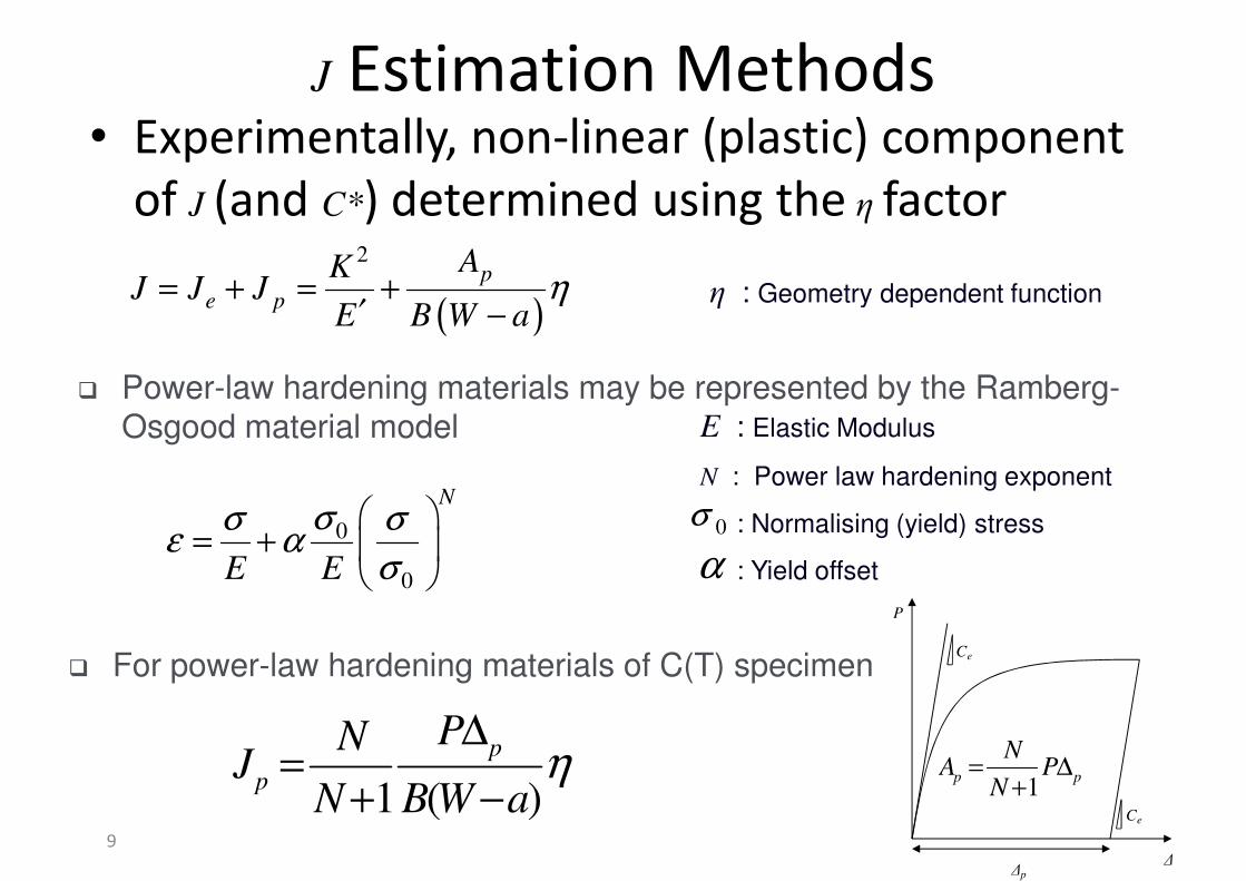
J Estimation Methods• Experimentally, non-linear (plastic) component
of J (and C*) determined using the η factor
( )
2p
e p
AKJ J J η= + = +
′ −η : Geometry dependent function
( )e pJ J JE B W a
η= + = +′ −
� Power-law hardening materials may be represented by the Ramberg-Osgood material model
0
0
N
E E
σσ σε α
σ
= +
E : Elastic Modulus
N : Power law hardening exponent
: Normalising (yield) stress
: Yield offset
0σ
α
η : Geometry dependent function
9
0
� For power-law hardening materials of C(T) specimen
1 ( )
p
p
PNJ
N B W aη
∆=
+ − 1p p
NA P
N= ∆
+
Ce
Ce
P
∆p
∆

η Factor for Weldments• Previous work to determine the η factors mainly
for homogenous materials
• Limited work has been performed on • Limited work has been performed on
weldments.
• Aim of this work was to determine the η factor
on C(T) specimen geometries for a range of:
– Crack lengths, a
Mismatch ratios,
PW2
LLD∆
– Mismatch ratios, M
– Weld widths, h
– Stress states : Plane Stress and Plane Strain
– Power-law hardening exponents, N10
P
a
2H 2h
2
LLD∆
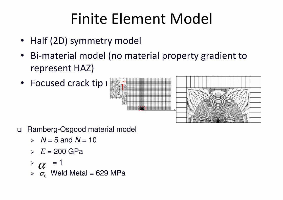
Finite Element Model
• Half (2D) symmetry model
• Bi-material model (no material property gradient to
represent HAZ)represent HAZ)
• Focused crack tip mesh design
� Ramberg-Osgood material model
� N = 5 and N = 10
� E = 200 GPa
� = 1
� Weld Metal = 629 MPaα
0σ
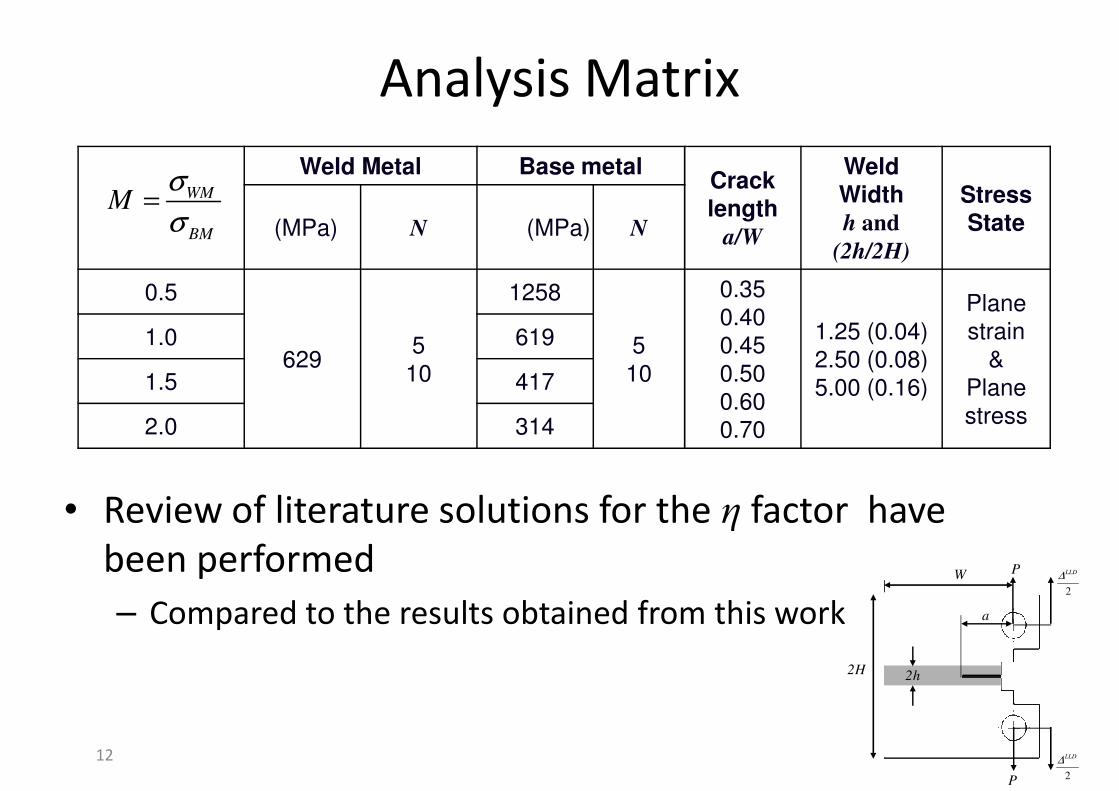
Analysis Matrix
Weld Metal Base metalCrack length
a/W
Weld Width h and
(2h/2H)
Stress State(MPa) N (MPa) N
WM
BM
Mσσ
=
• Review of literature solutions for the η factor have
0.5
6295
10
1258
510
0.350.400.45
0.500.600.70
1.25 (0.04)2.50 (0.08)5.00 (0.16)
Plane strain
&
Plane stress
1.0 619
1.5 417
2.0 314
• Review of literature solutions for the η factor have
been performed
– Compared to the results obtained from this work
12
P
a
PW
2H 2h
2
LLD∆
2
LLD∆

Specimen Geometries DefinitionSEN(T) M(T) DEN(T)
C(T) CS(T)SEN(B)
13P
a
PW
2H 2h
2
LLD∆
2
LLD∆

C(T): Best fits ηLLD
2.2
2.4
2.6
� For a given a/W and M for the conditions examined, η values found
to differ by a maximum of 12% of
0.30 0.35 0.40 0.45 0.50 0.55 0.60 0.65 0.70 0.751.4
1.6
1.8
2.0
2.2
a/W
ηL
LD
M=0.5
M=1.0
M=1.5
M=2.0
to differ by a maximum of 12% of
the mean value
� Mean values can describe
� a/W dependency of η
� influence of M for a given a/W
• ηmay be considered to be somewhat insensitive to
crack length for 0.4 ≤ a/W ≤ 0.7, for all M values
• For a given a/W , η decreases as M increases
14

CS(T): Best fits ηLLD and ηCMOD
2.6
2.8
3.0
L/W=2, h=2.5 mm
Plane stress and plane strain
with N= 5, 10, 20 M=0.5
M=1.0
M=1.5
M=2.0 4.2
4.4
4.6
4.8
5.0L/W=2, h=2.5 and 5 mm
Plane stress and plane strain
with N= 5, 10, 20 M=0.5
M=1.0
M=1.5
M=2.0
0.2 0.3 0.4 0.5 0.6 0.7
1.6
1.8
2.0
2.2
2.4
ηLLD
a/W
M=2.0
0.2 0.3 0.4 0.5 0.6 0.7
2.6
2.8
3.0
3.2
3.4
3.6
3.8
4.0
4.2
ηC
MO
D
a/W
15
• The investigations do not consider the different weld width.
• For a given crack length, the η solutions of the under-matched and over-
matched conditions show a less than 10% variation to homogeneous
material.
• Due to the good trends on both ηLLD and ηCMOD , both methods can be used to
evulate J and C*.
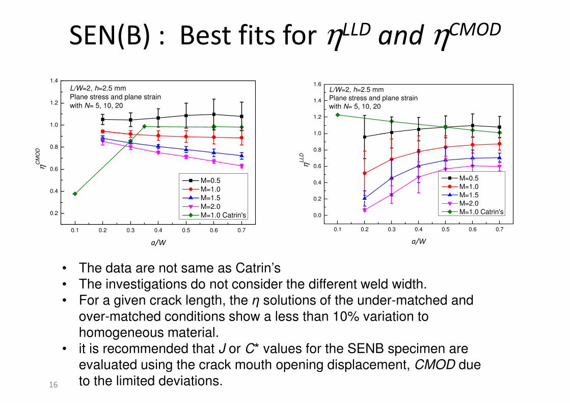
SEN(B) : Best fits for ηLLD and ηCMOD
1.0
1.2
1.4
L/W=2, h=2.5 mm
Plane stress and plane strain
with N= 5, 10, 20
1.0
1.2
1.4
1.6L/W=2, h=2.5 mm
Plane stress and plane strain
with N= 5, 10, 20
• The data are not same as Catrin’s
0.1 0.2 0.3 0.4 0.5 0.6 0.7
0.2
0.4
0.6
0.8
ηC
MO
D
a/W
M=0.5
M=1.0
M=1.5
M=2.0
M=1.0 Catrin's
0.1 0.2 0.3 0.4 0.5 0.6 0.7
0.0
0.2
0.4
0.6
0.8
1.0
M=0.5
M=1.0
M=1.5
M=2.0
M=1.0 Catrin's
ηLLD
a/W
16
• The data are not same as Catrin’s
• The investigations do not consider the different weld width.
• For a given crack length, the η solutions of the under-matched and
over-matched conditions show a less than 10% variation to
homogeneous material.
• it is recommended that J or C* values for the SENB specimen are
evaluated using the crack mouth opening displacement, CMOD due
to the limited deviations.
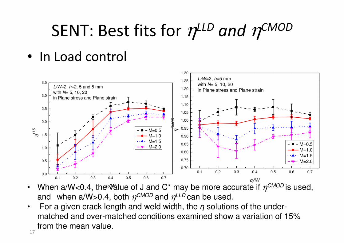
SENT: Best fits for ηLLD and ηCMOD
• In Load control
3.5 1.25
1.30
L/W=2, h=5 mm
0.5
1.0
1.5
2.0
2.5
3.0
3.5
L/W=2, h=2. 5 and 5 mm
with N= 5, 10, 20
in Plane stress and Plane strain
ηLLD M=0.5
M=1.0
M=1.5
M=2.0
0.75
0.80
0.85
0.90
0.95
1.00
1.05
1.10
1.15
1.20
1.25L/W=2, h=5 mm
with N= 5, 10, 20
in Plane stress and Plane strain
ηC
MO
D
M=0.5
M=1.0
M=1.5
M=2.0
17
0.1 0.2 0.3 0.4 0.5 0.6 0.70.0
0.5
a/W
0.1 0.2 0.3 0.4 0.5 0.6 0.70.70
0.75
a/W
M=2.0
• When a/W<0.4, the value of J and C* may be more accurate if ηCMOD is used,
and when a/W>0.4, both ηCMOD and ηLLD can be used.
• For a given crack length and weld width, the η solutions of the under-
matched and over-matched conditions examined show a variation of 15%
from the mean value.
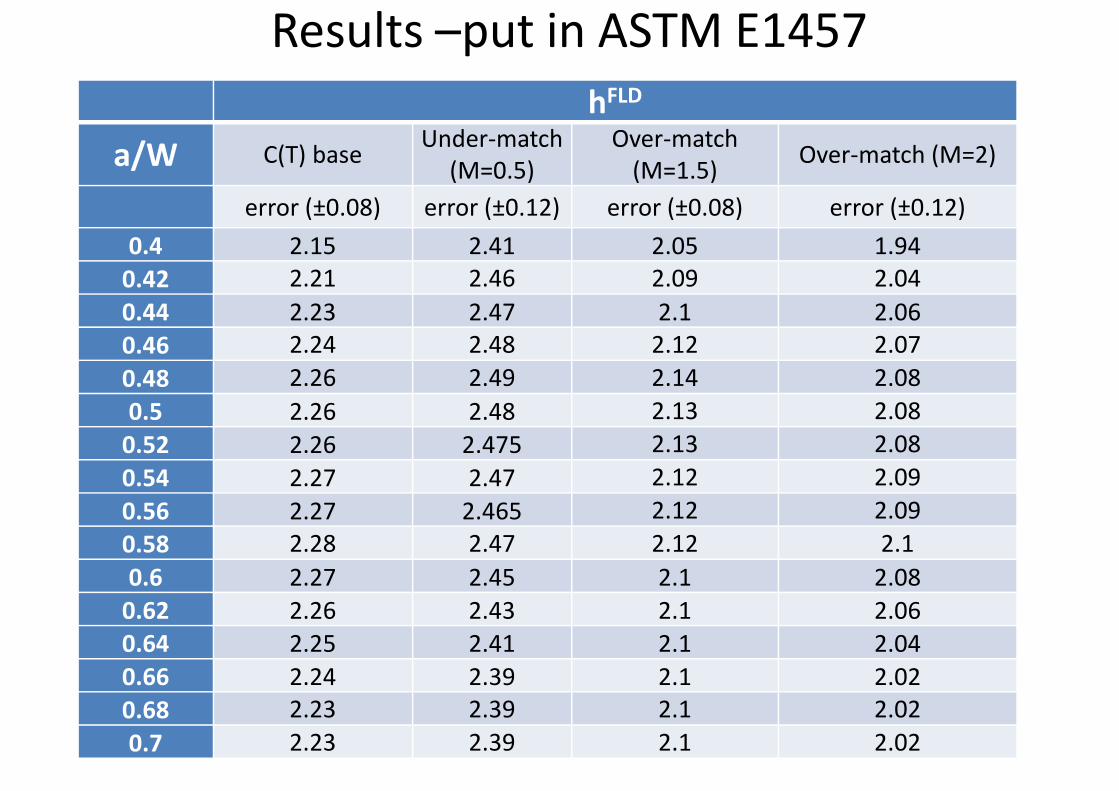
Results –put in ASTM E1457
hFLD
a/W C(T) baseUnder-match
(M=0.5)
Over-match
(M=1.5)Over-match (M=2)
error (±0.08) error (±0.12) error (±0.08) error (±0.12)
0.4 2.15 2.41 2.05 1.94
0.42 2.21 2.46 2.09 2.040.42 2.21 2.46 2.09 2.04
0.44 2.23 2.47 2.1 2.06
0.46 2.24 2.48 2.12 2.07
0.48 2.26 2.49 2.14 2.08
0.5 2.26 2.48 2.13 2.08
0.52 2.26 2.475 2.13 2.08
0.54 2.27 2.47 2.12 2.09
0.56 2.27 2.465 2.12 2.09
2.28 2.47 2.12 2.10.58 2.28 2.47 2.12 2.1
0.6 2.27 2.45 2.1 2.08
0.62 2.26 2.43 2.1 2.06
0.64 2.25 2.41 2.1 2.04
0.66 2.24 2.39 2.1 2.02
0.68 2.23 2.39 2.1 2.02
0.7 2.23 2.39 2.1 2.02
Quantitative measurements of residual stress
in Compact Tension specimens
• Examples of residual stress in CT and
welded components welded components
• Implications for
– Fracture parameters– Fracture parameters
– Life assessment
– Codes of practice
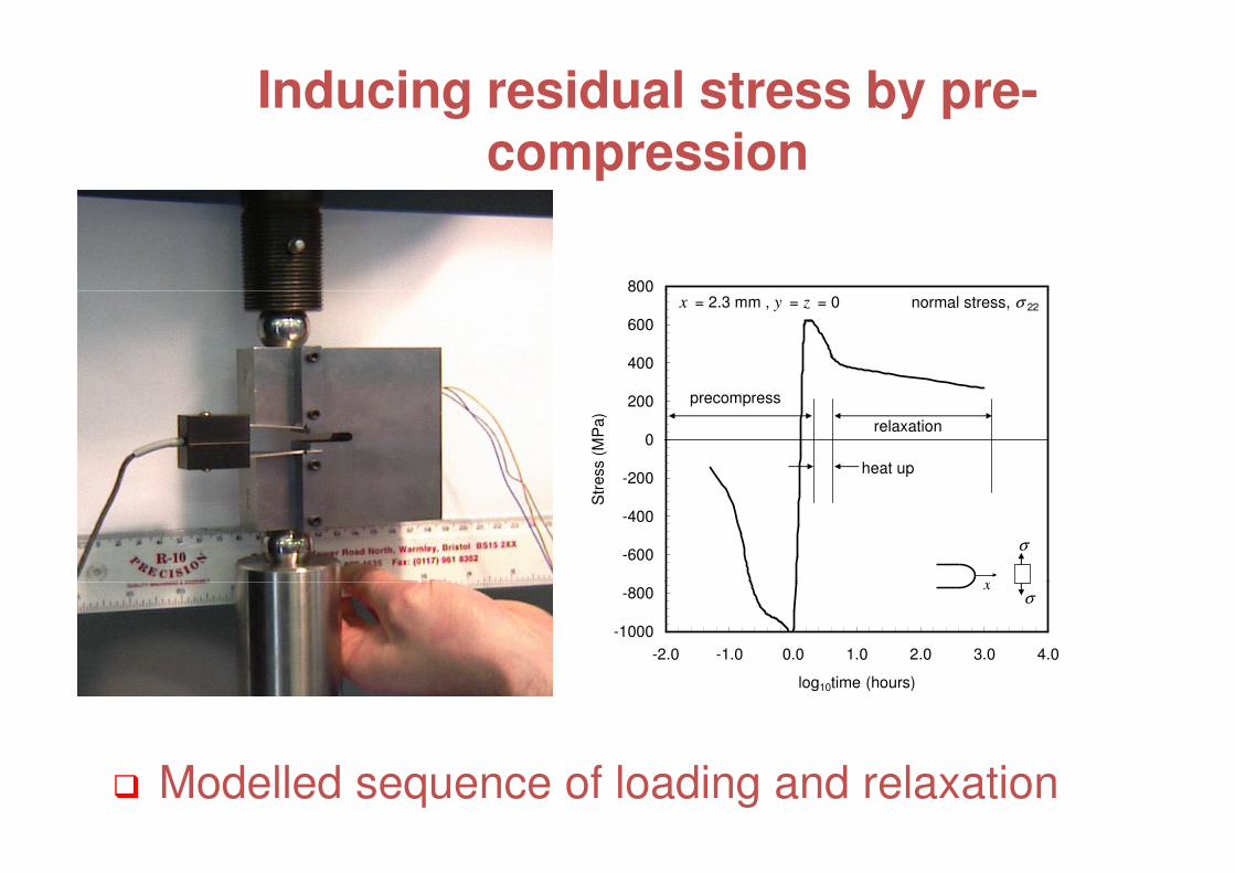
Inducing residual stress by pre-compression
800
-600
-400
-200
0
200
400
600
800
Str
ess (
MP
a)
x = 2.3 mm , y = z = 0
x
σ
normal stress, σ 22
relaxation
heat up
precompress
� Modelled sequence of loading and relaxation
-1000
-800
-2.0 -1.0 0.0 1.0 2.0 3.0 4.0
log10time (hours)
xσ

Residual stress due to welding
Starter Crack
Parent Metal
W
P
W
P
HAZ
a) b)
� 316L Weld Metal, P22, P91, P92 HAZ and weld test
� EDM notch located in Heat Affected Zone (HAZ)
Weld Metal
a
P
a
P
� EDM notch located in Heat Affected Zone (HAZ)
� EDM or Pre-fatigued starter crack
� As-welded condition (non-stress relieved)
� Size and geometry effects
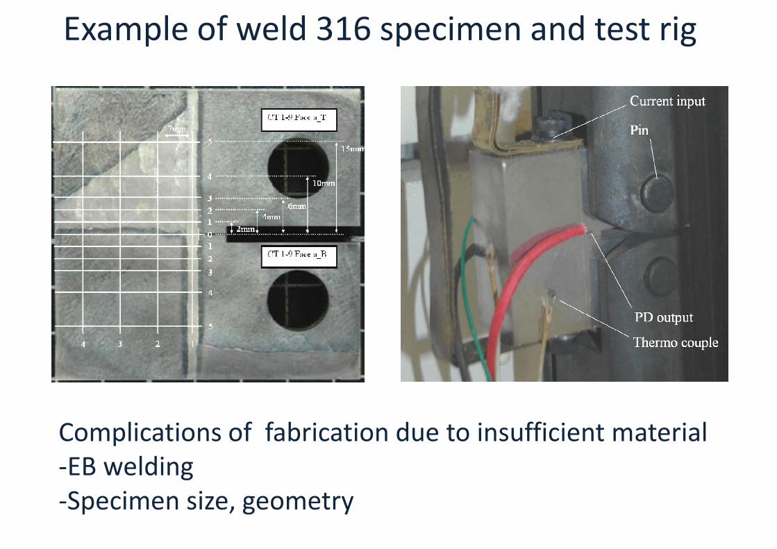
Example of weld 316 specimen and test rig
a) b)
Complications of fabrication due to insufficient material
-EB welding
-Specimen size, geometry

Measurement Details
Parent
2 mm 4 mm
EB WeldScan II EB Weld
(a)(b)
Slice cut line
62.5 mm Scan IV
� Specimen EB1 � Specimen EB2
Parent
x 11
x 22
x 33
EB Weld
x 11 = 0
Scan I
Scan II
Parent
EB Weld
x 11 = 0
Scan III
Parent
EDM 1
EDM 2
Slice cut line
MMA Weld MMA Weld
60 m
m
• Specimen EB1 unslit
• EDM slit in specimen EB2
– EDM1 : a/W = 0.5
– EDM2 : a/W = 0.57
• Measurement along expected crack path 23
x 11 = 0 x 11 = 0

Residual Stress in welded CT
600
800
σ22
σ33
σ11
EB1(b)
σ 22
σ 33
σ 11
400
600
800
σ22
σ33
σ11
EB2 EDM1(b)
σ 22
σ 33
σ 11
-400
-200
0
200
400
Str
ess
(MP
a)
-400
-200
0
200
400
-30.0 -20.0 -10.0 0.0 10.0 20.0 30.0
Str
ess
(MP
a)
24
-30.0 -20.0 -10.0 0.0 10.0 20.0 30.0
Distance from EB Weld (mm)
-30.0 -20.0 -10.0 0.0 10.0 20.0 30.0
Distance from EB Weld (mm)
• Significant stress relaxation with EDM slit
introduction 30-50 % reduction

Effect of Residual Stress
400
600
800
Re
sid
ual
Str
ess (
MP
a)
s22 Stress-Spec no crack
s22 Stress-Spec crack
s22 Stress-Spec crack 2
Crack 1
EB Weld
Weld multipass region (see Fig. 5.1)
σ22: no crackσ22: crack 1σ22: crack 2
Measurement line
x
-400
-200
0
200
0 10 20 30 40 50 60
Position (mm)
Re
sid
ual
Str
ess (
MP
a)
Crack 2
HAZ
a
12.5 mm
� residual stress profiles before testing in a weldment
� Large effect due to the EB weld reduces with crack growth
� Most of the residual stress is removed when crack is extended
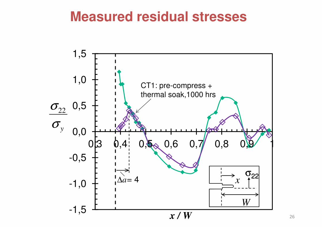
Measured residual stresses
1,0
1,5
0,0
0,5
1,0
0,3 0,4 0,5 0,6 0,7 0,8 0,9 1
CT1: pre-compress +
thermal soak,1000 hrs
yσσ22
26-1,5
-1,0
-0,5
x / W
∆a= 4
W
σ22σ22x

Measured residual stresses
1,0
1,5
CT2: Pre-compress + EDM 2 mm crack
0,0
0,5
1,0
0,3 0,4 0,5 0,6 0,7 0,8 0,9 1
yσσ22
27-1,5
-1,0
-0,5
x / W
∆a= 2
W
σ22σ22x

Measured residual stresses
1,0
1,5
CT2: Pre-compress + EDM 2 mm crack +
primary load, 650°C, 1000 hrs
0,0
0,5
1,0
0,3 0,4 0,5 0,6 0,7 0,8 0,9 1
yσσ22
primary load, 650°C, 1000 hrs
28-1,5
-1,0
-0,5
x / W
∆ a = 15W
σ22σ22x

Measured residual stresses
1,0
1,5
0,0
0,5
1,0
0,3 0,4 0,5 0,6 0,7 0,8 0,9 1
yσσ22
29-1,5
-1,0
-0,5
x / W
W
σ22σ22x
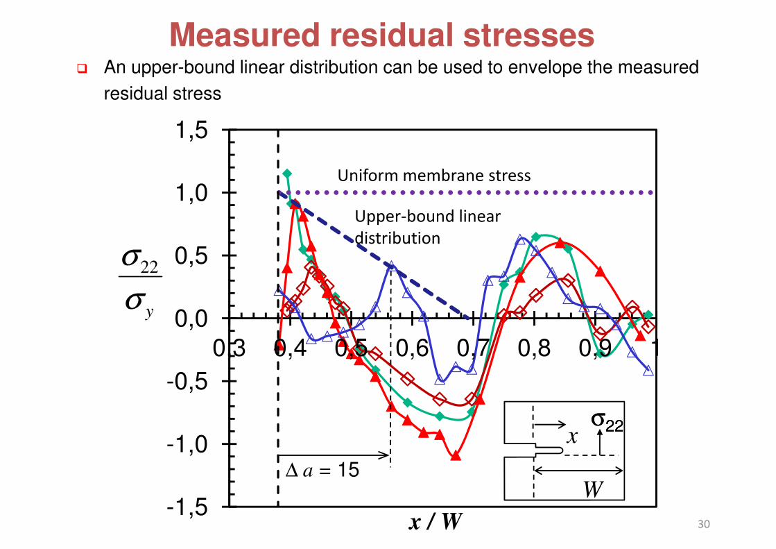
Measured residual stresses
1,0
1,5
� An upper-bound linear distribution can be used to envelope the measured
residual stress
Uniform membrane stress
0,0
0,5
1,0
0,3 0,4 0,5 0,6 0,7 0,8 0,9 1
yσσ22
Uniform membrane stress
Upper-bound linear
distribution
30-1,5
-1,0
-0,5
x / W
∆ a = 15W
σ22σ22x
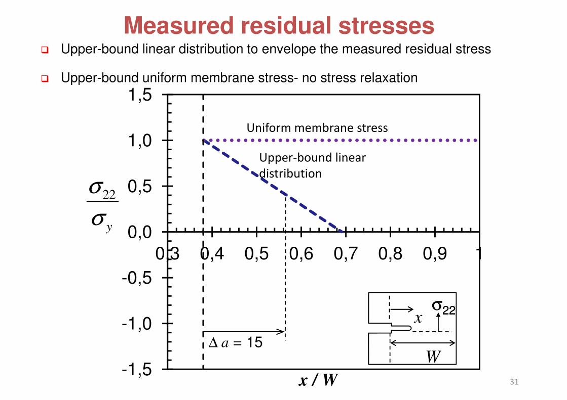
Measured residual stresses
1,0
1,5
� Upper-bound linear distribution to envelope the measured residual stress
� Upper-bound uniform membrane stress- no stress relaxation
Uniform membrane stress
0,0
0,5
1,0
0,3 0,4 0,5 0,6 0,7 0,8 0,9 1
yσσ22
Uniform membrane stress
Upper-bound linear
distribution
31-1,5
-1,0
-0,5
x / W
∆ a = 15W
σ22σ22x
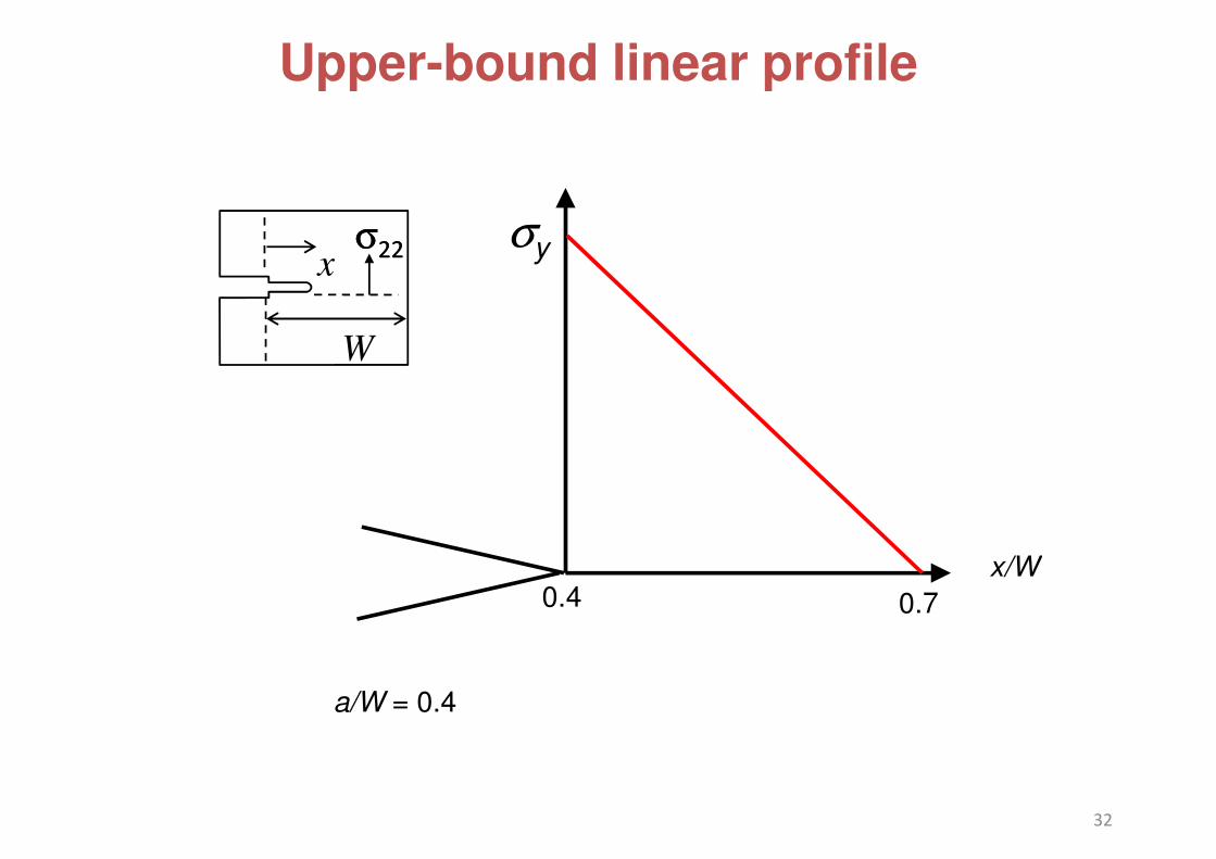
Upper-bound linear profile
σ22σ22x
σy
W
x/W
32
a/W = 0.4
x/W0.4 0.7

Upper-bound linear profile
σ22σ22x
σy
W
x/W
0.67σy
33
a/W = 0.5
x/W
0.5 0.7

Upper-bound linear profile
σ22σ22x
σy
W
x/W
0.67σy
0.33σy
34
a/W = 0.6
x/W
0.6 0.7

Introduction of residual stress� Residual stress introduced as an initial stress distribution using the
SIGINI subroutine in Abaqus
� Arbitrary ‘balancing’ stress required to give force and moment equilibrium
0,6
0
0,1
0,2
0,3
0,4
0,5
σ2
2 /
σy
35� Two-dimensional elastic 2D elastic analysis performed
-0,3
-0,2
-0,1
0
0,5 0,6 0,7 0,8 0,9 1
σ
x/W

Introduction of crack in FE model� Crack is introduced by releasing boundary constraint on nodes
over a distance of x/W = 0.02 of crack tip
0,6
0
0,1
0,2
0,3
0,4
0,5
σ2
2 /
σy
x/W = 0.02
36
-0,3
-0,2
-0,1
0
0,5 0,6 0,7 0,8 0,9 1
x/W
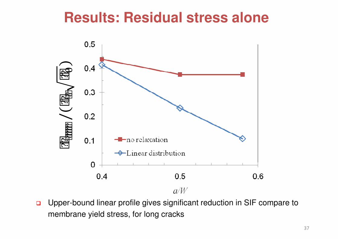
Results: Residual stress alone
��� 0
) ��
������
/(�
� ���
��
37
� Upper-bound linear profile gives significant reduction in SIF compare to
membrane yield stress, for long cracks

Residual stress + primary load
F =14.5 kN
� Residual stress combined with primary load of 14.5 kN,
corresponds to Kp =15 MPa √m for a/W = 0.4
F =14.5 kN
38
� using upper-bound linear profile is too conservative
when residual stress is combined with primary load
Quantitative measurements of residual stress
ion components
• Examples of residual stress in various
components and methods of Residual components and methods of Residual
Stress measurement
• Implications on • Implications on
– K and C* parameters
– Life assessment
– Codes of practice
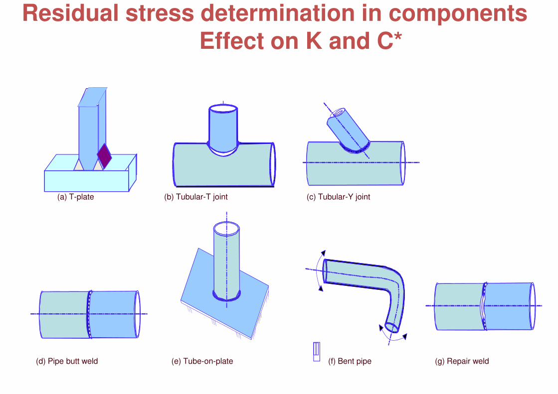
Residual stress determination in componentsEffect on K and C*
(a) T-plate (b) Tubular-T joint (c) Tubular-Y joint
(d) Pipe butt weld (e) Tube-on-plate (f) Bent pipe (g) Repair weld

Comparison of measured distributions
with chosen profiles
T-plate 1
1.2
∪⊥∅
∪ y
data (S E 702)
data (S 355)
R6 / B S 7910(2)re
sid
ual str
ess,
σ
σ
σ σ /
σσ σσy
0
0.2
0.4
0.6
0.8
norm
alis
ed r
esid
ual str
ess, ∪
⊥∅R6 / B S 7910(2)
B S 7910 (1)
B ilinear [3]
a
No
rmalised
resid
ual str
ess,
-0.4
-0.2
0 0.2 0.4 0.6 0.8 1y /W
norm
alis
ed r
esid
ual str
ess,
No
rmalised

Residual Stress Measurement on T-plate
1
1.5
Force balanced data (average)As received data (average)Bi-linear approximation of averageBi-linear approximation of average +0.25
No
rma
lise
d R
esid
ua
l S
tre
ss (
σre
s/σY
P)
-0.5
0
0.5
No
rma
lise
d R
esid
ua
l S
tre
ss (
MeanMean + 2sdv
yW
� Upper bound distribution is less conservative than current
BS7910 and R6 level 1 and 2 distributions
-0.5
0 0.2 0.4 0.6 0.8 1
Normalised Position (y/w)
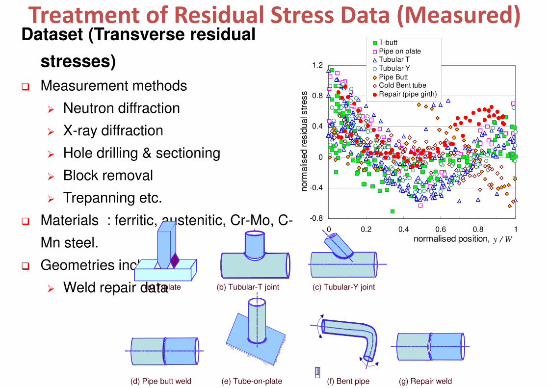
Dataset (Transverse residual
stresses)
� Measurement methods
� Neutron diffraction
� X-ray diffraction 0.4
0.8
1.2
norm
alis
ed r
esid
ual s
tress
T-butt
Pipe on plateTubular T
Tubular Y
Pipe ButtCold Bent tube
Repair (pipe girth)
Treatment of Residual Stress Data (Measured)
� X-ray diffraction
� Hole drilling & sectioning
� Block removal
� Trepanning etc.
� Materials : ferritic, austenitic, Cr-Mo, C-
Mn steel.
Geometries included
-0.8
-0.4
0
0.4
0 0.2 0.4 0.6 0.8 1
normalised position, y / W
norm
alis
ed r
esid
ual s
tress
� Geometries included
� Weld repair data(a) T-plate (b) Tubular-T joint (c) Tubular-Y joint
(d) Pipe butt weld (e) Tube-on-plate (f) Bent pipe (g) Repair weld

0.8
1.2
norm
alis
ed r
esid
ual s
tress
T-butt
Pipe on plateTubular T
Tubular Y
Pipe ButtCold Bent tube
Repair (pipe girth)
Caution: Scatter in Experimental and FEM results
-0.8
-0.4
0
0.4
0 0.2 0.4 0.6 0.8 1
normalised position, y / W
norm
alis
ed r
esid
ual s
tress
Caution should be exercised in Life Assessment
Analysis in FEM of Measurements of
in Residual stress in Residual stress
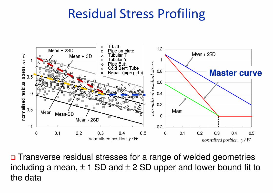
Residual Stress Profiling
1
1.2
no
rma
lise
d r
esi
du
al
stre
ss
Mean + 2SD
-0.2
0
0.2
0.4
0.6
0.8
no
rma
lise
d r
esi
du
al
stre
ss
Master curve
Mean
Master curve
� Transverse residual stresses for a range of welded geometries
including a mean, ± 1 SD and ± 2 SD upper and lower bound fit to
the data
-0.2
0 0.1 0.2 0.3 0.4 0.5
normalised position, y / W
0.8
π↑°�
y
Linear Upper Bound
Linear Lower Bound
Proposed Linear (0.75)
resid
ual str
ess,
σσ σσ/ σσ σσ
y
2data (S355)Linear Upper BoundLinear Lower Bound σ σ σ σ
y√π√π √π√
πa
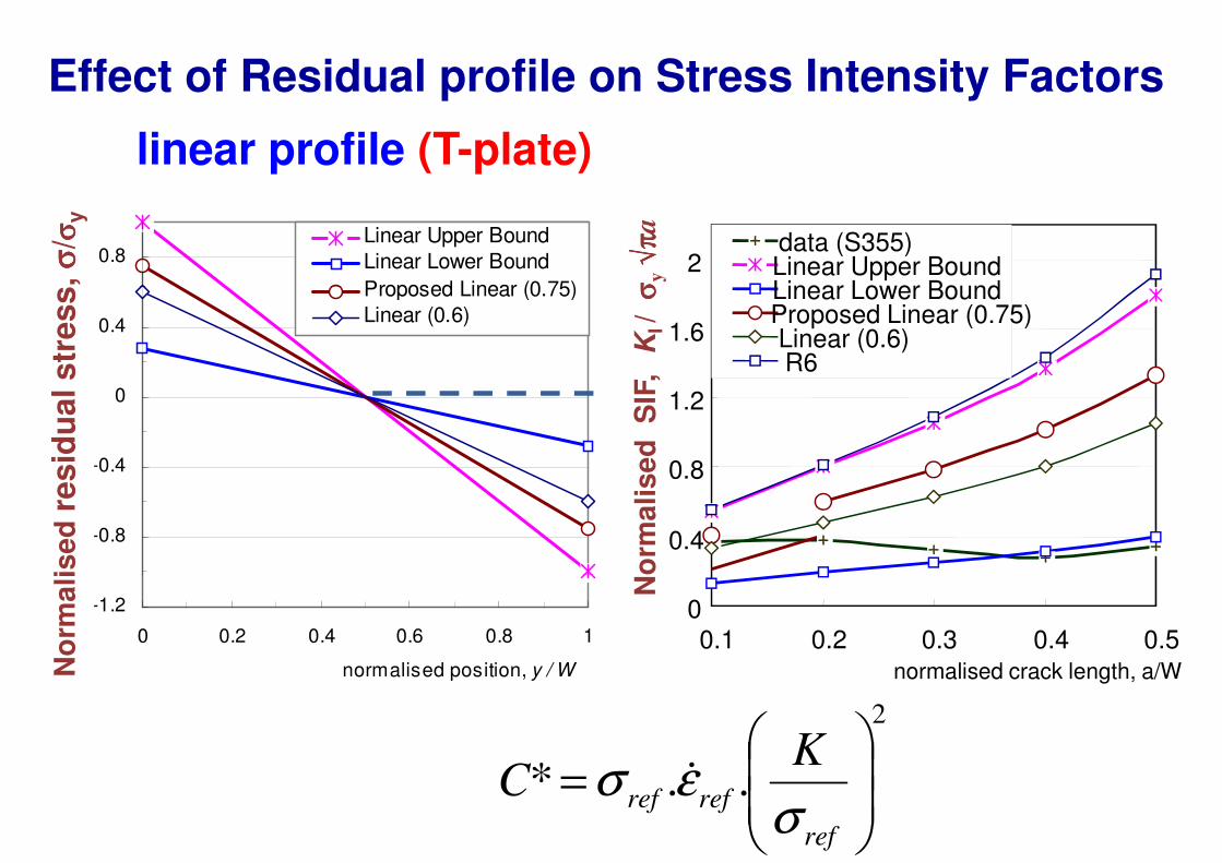
Effect of Residual profile on Stress Intensity Factors
linear profile (T-plate)
-0.8
-0.4
0
0.4
no
rma
lise
d r
esid
ua
l str
ess
, π↑° Proposed Linear (0.75)
Linear (0.6)
No
rma
lis
ed
resid
ual str
ess,
0.4
0.8
1.2
1.6
Linear Lower BoundProposed Linear (0.75)Linear (0.6)R6
No
rma
lis
ed
SIF
,K
I /
σ σ σ σ
-1.2
0 0.2 0.4 0.6 0.8 1
normalised position, y / WNo
rma
lis
ed
00.1 0.2 0.3 0.4 0.5
normalised crack length, a/WN
orm
ali
se
d
2
..*
=
ref
refref
KC
σεσ ɺ
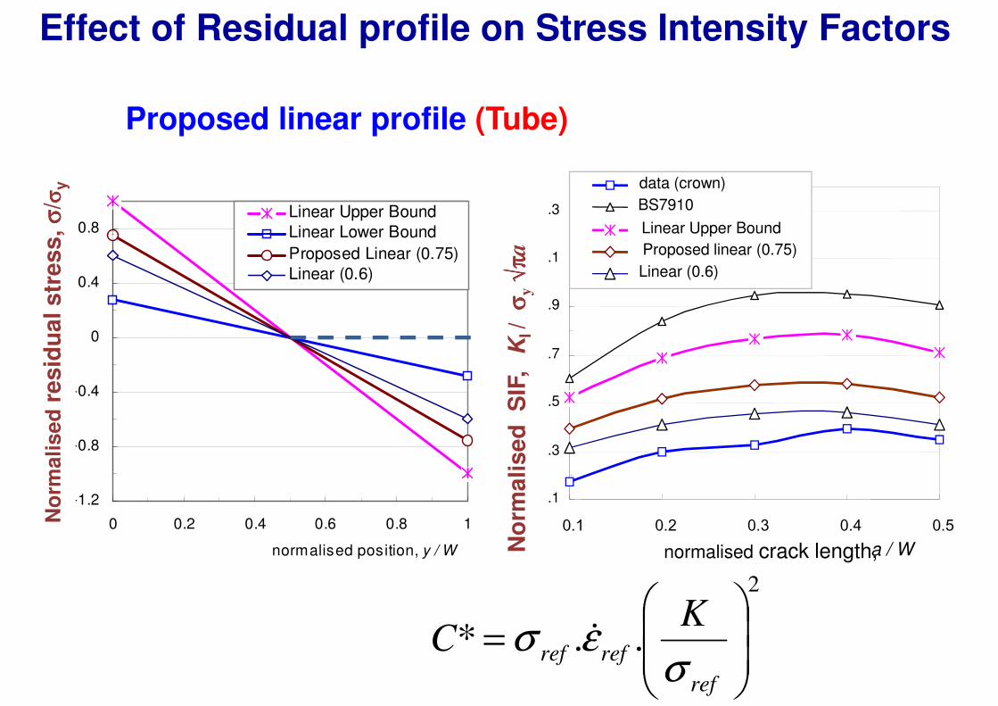
Proposed linear profile (Tube)
1.3
data (crown)
BS7910
Linear Upper Bound
Effect of Residual profile on Stress Intensity Factors
0.8
y
Linear Upper Bound
Linear Lower Bound
res
idu
al s
tre
ss
, σσ σσ
/ σσ σσy
0.3
0.5
0.7
0.9
1.1
Linear Upper Bound
Proposed linear (0.75)
Linear (0.6)
No
rma
lis
ed
SIF
,K
I /
σ σ σ σy
√π√π √π√πa
-0.8
-0.4
0
0.4
0.8
no
rma
lise
d r
esid
ua
l str
ess
, π↑°�
y
Linear Lower Bound
Proposed Linear (0.75)
Linear (0.6)
No
rma
lis
ed
res
idu
al s
tre
ss
,
0.1
0.1 0.2 0.3 0.4 0.5normalised crack length, a / WN
orm
ali
se
d-1.2
0 0.2 0.4 0.6 0.8 1
normalised position, y / W
No
rma
lis
ed
2
..*
=
ref
refref
KC
σεσ ɺ

To Improve Testing and Assessment Codes for Welds
• Provide comprehensive and validated data
• Provide improved parameters to assess cracks• Provide improved parameters to assess cracks
• Development of predictive numerical tools for
welds
• Validation and verification of modelling, testing • Validation and verification of modelling, testing
for component

Standards that need to be updated
• ASTM E1457-2012 ‘Creep Crack Growth testing
Standard’,
• Nikbin, K. M, ‘Creep Crack Growth Life Assessment’, • Nikbin, K. M, ‘Creep Crack Growth Life Assessment’,
PVRC Document’, 2007
• ISO/TTA 2007(E) – ‘Creep/Fatigue Crack growth
Testing of Components’
• ASTM E2670 ‘Creep/Fatigue Crack Growth Testing• ASTM E2670 ‘Creep/Fatigue Crack Growth Testing
• Under the auspices of VAMAS TWA31- Committee
for Creep/Fatigue Cracking in Weldments