Embed Size (px)
Citation preview
Mathematical Methodsfor Computer Graphics
Christian Lessig


“It is through science that we prove,but through intuition that we discover.”
Henri Poincaré

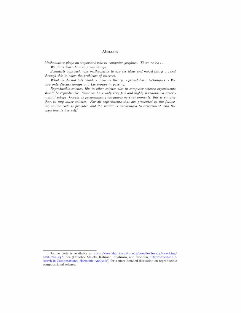
Abstract
Mathematics plays an important role in computer graphics. These notes . . .We don’t learn how to prove things.Scientists approach: use mathematics to express ideas and model things . . . and
through this to solve the problems of interest.What we do not talk about: - measure theory. - probabilistic techniques. - We
also only discuss groups and Lie groups in passing.Reproducible science: like in other science also in computer science experiments
should be reproducible. Since we have only very few and highly standardized experi-mental setups, known as programming languages or environments, this is simplerthan in any other science. For all experiments that are presented in the follow-ing source code is provided and the reader is encouraged to experiment with theexperiments her self.1
1Source code is available at http://www.dgp.toronto.edu/people/lessig/teaching/math_for_cg/. See (Donoho, Maleki, Rahman, Shahram, and Stodden, “Reproducible Re-search in Computational Harmonic Analysis”) for a more detailed discussion on reproduciblecomputational science.

Contents
Contents vii
1 Linear Algebra 11.1 Linear Spaces . . . . . . . . . . . . . . . . . . . . . . . . . . . . 11.2 Linear Spaces with Additional Structure . . . . . . . . . . . . . 1
1.2.1 Norms . . . . . . . . . . . . . . . . . . . . . . . . . . . . 11.2.2 Inner Products . . . . . . . . . . . . . . . . . . . . . . . 1
1.3 Linear Functionals . . . . . . . . . . . . . . . . . . . . . . . . . 11.4 Bases for Linear Spaces . . . . . . . . . . . . . . . . . . . . . . 1
1.4.1 Biorthogonal Bases . . . . . . . . . . . . . . . . . . . . . 11.4.2 Orthonormal Bases . . . . . . . . . . . . . . . . . . . . . 21.4.3 Overcomplete Bases: Frames . . . . . . . . . . . . . . . 2
1.5 Linear Maps . . . . . . . . . . . . . . . . . . . . . . . . . . . . . 21.5.1 Fundamental Concepts . . . . . . . . . . . . . . . . . . . 21.5.2 Eigen and Singular Value Decomposition . . . . . . . . 11
1.6 Linear Spaces as Groups . . . . . . . . . . . . . . . . . . . . . . 201.7 Affine Spaces . . . . . . . . . . . . . . . . . . . . . . . . . . . . 221.8 Further Reading . . . . . . . . . . . . . . . . . . . . . . . . . . 23
2 Signal Processing and Applied Functional Analysis 252.1 Functions as Vectors in a Linear Space . . . . . . . . . . . . . . 252.2 Bases and Numerical Computations . . . . . . . . . . . . . . . 30
2.2.1 Orthonormal Bases . . . . . . . . . . . . . . . . . . . . . 312.2.2 Biorthogonal Bases and Frames . . . . . . . . . . . . . . 32
2.3 Approximation of Functions . . . . . . . . . . . . . . . . . . . . 342.3.1 Linear Approximation . . . . . . . . . . . . . . . . . . . 352.3.2 Nonlinear Approximation . . . . . . . . . . . . . . . . . 362.3.3 From One to Higher Dimensions . . . . . . . . . . . . . 39
2.4 Reproducing Kernels . . . . . . . . . . . . . . . . . . . . . . . . 402.4.1 Point Evaluation Functionals . . . . . . . . . . . . . . . 412.4.2 Reproducing Kernel Bases . . . . . . . . . . . . . . . . . 442.4.3 Choice of Sampling Points . . . . . . . . . . . . . . . . . 452.4.4 Pointwise Numerical Techniques . . . . . . . . . . . . . 46
2.5 Linear Operators on Function Spaces . . . . . . . . . . . . . . . 512.5.1 Differential Operators . . . . . . . . . . . . . . . . . . . 51
vii
2.5.2 Integral Operators . . . . . . . . . . . . . . . . . . . . . 572.5.3 Galerkin Projection . . . . . . . . . . . . . . . . . . . . 612.5.4 Fourier Theory Revisited . . . . . . . . . . . . . . . . . 67
2.6 Further Reading . . . . . . . . . . . . . . . . . . . . . . . . . . 68
3 Manifolds and Tensors 713.1 Preliminaries . . . . . . . . . . . . . . . . . . . . . . . . . . . . 713.2 Manifolds . . . . . . . . . . . . . . . . . . . . . . . . . . . . . . 72
3.2.1 Continuous Theory . . . . . . . . . . . . . . . . . . . . . 723.2.2 Discrete Theory . . . . . . . . . . . . . . . . . . . . . . 72
3.3 Tensors . . . . . . . . . . . . . . . . . . . . . . . . . . . . . . . 723.4 Differential Forms and Exterior Calculus . . . . . . . . . . . . . 73
3.4.1 Continuous Theory . . . . . . . . . . . . . . . . . . . . . 733.4.2 Discrete Theory . . . . . . . . . . . . . . . . . . . . . . 73
3.5 The Lie Derivative . . . . . . . . . . . . . . . . . . . . . . . . . 733.6 Riemannian Manifolds . . . . . . . . . . . . . . . . . . . . . . . 73
3.6.1 Continuous Theory . . . . . . . . . . . . . . . . . . . . . 733.6.2 Discrete Theory . . . . . . . . . . . . . . . . . . . . . . 73
3.7 Lie Groups . . . . . . . . . . . . . . . . . . . . . . . . . . . . . 733.7.1 The Euclidean Group . . . . . . . . . . . . . . . . . . . 733.7.2 The Rotation Group . . . . . . . . . . . . . . . . . . . . 733.7.3 Diffeomorphism Groups . . . . . . . . . . . . . . . . . . 73
3.8 Further Reading . . . . . . . . . . . . . . . . . . . . . . . . . . 73
4 Dynamical Systems and Geometric Mechanics 754.1 Motivation and Intuition . . . . . . . . . . . . . . . . . . . . . . 754.2 Ordinary and Partial Differential Equations . . . . . . . . . . . 754.3 Hamiltonian Mechanics . . . . . . . . . . . . . . . . . . . . . . 75
4.3.1 Continuous Theory . . . . . . . . . . . . . . . . . . . . . 754.3.2 Symplectic Integrators . . . . . . . . . . . . . . . . . . . 75
4.4 Lagrangian Mechanics . . . . . . . . . . . . . . . . . . . . . . . 754.4.1 Continuous Theory . . . . . . . . . . . . . . . . . . . . . 754.4.2 Variational Integrators . . . . . . . . . . . . . . . . . . . 76
4.5 Symmetries . . . . . . . . . . . . . . . . . . . . . . . . . . . . . 784.6 Further Reading . . . . . . . . . . . . . . . . . . . . . . . . . . 78
Bibliography 81
Index 87
viii


Chapter 1
Linear Algebra
Linear algebra is an elementary pillar of computer graphics, as is evident by thecentral place it takes in introductory computer graphics classes. In the following,however, we will consider some aspects that are usually not emphasized incomputer graphics but that play important roles for us in subsequent chapters.
1.1 Linear Spaces
Definition 1.1.
1.2 Linear Spaces with Additional Structure
1.2.1 Norms
Banach space: Remark on separability.
1.2.2 Inner Products
Hilbert space: Remark on separability.
1.3 Linear Functionals
Theorem 1.1.
1.4 Bases for Linear Spaces
Define: - linear independence - span of a set of vectors. - dimension of a vectorspace.
1.4.1 Biorthogonal Bases
- Schauder basis. - Hamel basis.
1
2
1.4.2 Orthonormal Bases
1.4.3 Overcomplete Bases: Frames
Example 1. Mercedes Benz frame
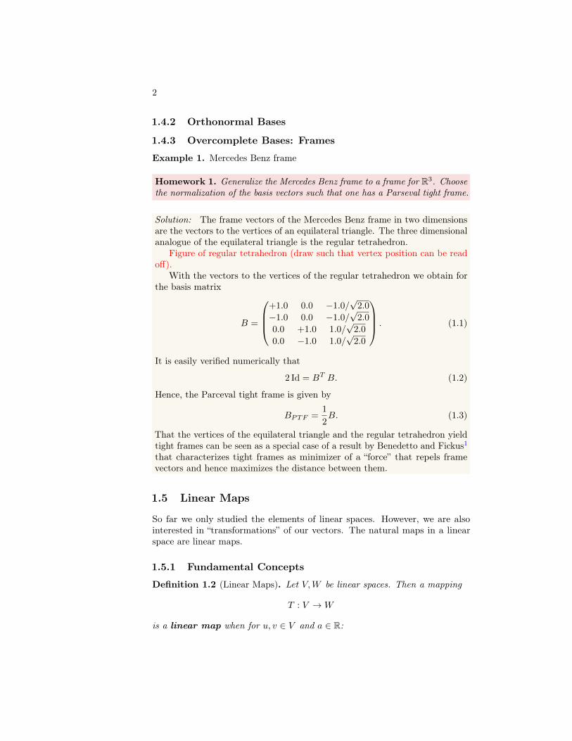
Homework 1. Generalize the Mercedes Benz frame to a frame for R3. Choosethe normalization of the basis vectors such that one has a Parseval tight frame.
Solution: The frame vectors of the Mercedes Benz frame in two dimensionsare the vectors to the vertices of an equilateral triangle. The three dimensionalanalogue of the equilateral triangle is the regular tetrahedron.
Figure of regular tetrahedron (draw such that vertex position can be readoff).
With the vectors to the vertices of the regular tetrahedron we obtain forthe basis matrix
B =
+1.0 0.0 −1.0/
√2.0
−1.0 0.0 −1.0/√
2.0
0.0 +1.0 1.0/√
2.0
0.0 −1.0 1.0/√
2.0
. (1.1)
It is easily verified numerically that
2 Id = BT B. (1.2)
Hence, the Parceval tight frame is given by
BPTF =1
2B. (1.3)
That the vertices of the equilateral triangle and the regular tetrahedron yieldtight frames can be seen as a special case of a result by Benedetto and Fickus1that characterizes tight frames as minimizer of a “force” that repels framevectors and hence maximizes the distance between them.
1.5 Linear Maps
So far we only studied the elements of linear spaces. However, we are alsointerested in “transformations” of our vectors. The natural maps in a linearspace are linear maps.
1.5.1 Fundamental Concepts
Definition 1.2 (Linear Maps). Let V,W be linear spaces. Then a mapping
T : V →W
is a linear map when for u, v ∈ V and a ∈ R:
3
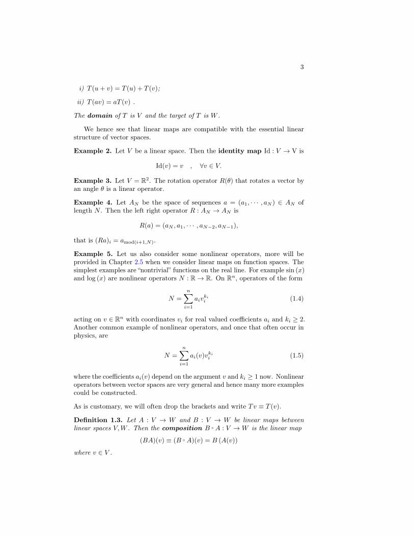
i) T (u+ v) = T (u) + T (v);
ii) T (av) = aT (v) .
The domain of T is V and the target of T is W .
We hence see that linear maps are compatible with the essential linearstructure of vector spaces.
Example 2. Let V be a linear space. Then the identity map Id : V → V is
Id(v) = v , ∀v ∈ V.
Example 3. Let V = R2. The rotation operator R(θ) that rotates a vector byan angle θ is a linear operator.
Example 4. Let AN be the space of sequences a = (a1, · · · , aN ) ∈ AN oflength N . Then the left right operator R : AN → AN is
R(a) = (aN , a1, · · · , aN−2, aN−1),
that is (Ra)i = amod(i+1,N).
Example 5. Let us also consider some nonlinear operators, more will beprovided in Chapter 2.5 when we consider linear maps on function spaces. Thesimplest examples are “nontrivial” functions on the real line. For example sin (x)and log (x) are nonlinear operators N : R→ R. On Rn, operators of the form
N =
n∑i=1
aivkii (1.4)
acting on v ∈ Rn with coordinates vi for real valued coefficients ai and ki ≥ 2.Another common example of nonlinear operators, and once that often occur inphysics, are
N =
n∑i=1
ai(v)vkii (1.5)
where the coefficients ai(v) depend on the argument v and ki ≥ 1 now. Nonlinearoperators between vector spaces are very general and hence many more examplescould be constructed.
As is customary, we will often drop the brackets and write Tv ≡ T (v).
Definition 1.3. Let A : V → W and B : V → W be linear maps betweenlinear spaces V,W . Then the composition B A : V →W is the linear map
(BA)(v) ≡ (B A)(v) = B (A(v))
where v ∈ V .
4
One often writes AB without specifying a vector. When it is unclear what thismeans one should recall the definition in terms of the action on vectors. Thefollowing two concepts are important in many applications.
Definition 1.4 (kernel,range,). Let V,W be linear spaces and T : V →W bea linear map. Then the kernel ker(T ) of T is
ker(T ) = v ∈ V | T (v) = 0 .
Then range ran(T ) (or image) is
ran(T ) = w ∈W | ∃v ∈ V : T (v) = w .
It is usually important to distinguish the target and range of an operator andthey coincide only in special cases.
Theorem 1.2 (Rank-Nullity Theorem). Let V,W be linear spaces and T : V →W be a linear map. Then
dim(ker(T )) + dim(ran(T )) = dim (V ).
The dimension dim(ran(T )) of the range of T is the rank of T
rank(T ) = dim(ran(T )).
We have established the essential properties of linear maps on vector spacesbut not discussed how to work numerically with them. Without loss of generality,let V be a Hilbert space and T : V → V be a linear map. Furthermore, leteiNi=1 be an orthonormal basis for V so that for any v ∈ V we have
v =
N∑i=1
vi ei =
N∑i=1
〈v, ei〉 . (1.6)
Then for the linear map T applied to v we have
T (v) = T
(N∑i=1
vi ei
)(1.7a)
and by linearity of T with respect to vector addition this equals
T (v) =
N∑i=1
T (vi ei). (1.7b)
Also using linearity with respect to scalar multiplication by the vi we obtain
T (v) =
N∑i=1
vi T (ei). (1.7c)
5
Hence, the action of T on v is fully determined by the action on the basisvectors ei. This should not come as a surprise since the ei are, through theirlinear superposition, equivalent to any vector v.
T (v) in the above form is not useful numerically. For this, we also need thecoordinate representation of the image v = T (v). As we have seen before, wehave vj = 〈ej , v〉. Hence,
〈ej , T (v)〉 =
⟨ej ,
N∑i=1
vi T (ei)
⟩(1.8a)
and by the linearity of the inner product we have
〈ej , T (v)〉 =N∑i=1
〈ej , vi T (ei)〉 (1.8b)
=
N∑i=1
vi 〈ej , T (ei)〉 (1.8c)
By defining
〈ej , T (v)〉 =
N∑i=1
vi 〈ej , T (ei)〉︸ ︷︷ ︸Tji
(1.8d)
we obtain
〈ej , T (v)〉 =
N∑i=1
Tjivi (1.8e)
If we collect the coefficients Tji in a two-dimensional “array” and the vj and viinto one-dimensional ones then we obtain v1
...vN
=
T11 · · · T1N
.... . .
...TN1 · · · TNN
v1
...vN
. (1.9)
The foregoing derivation shows that matrices are the coordinate representationof linear operators. In computer science, matrices are often said to be linearoperators. However, as we will see in the following it is useful, and at timesimportant, to distinguish linear operators and their representations as matrices.
Homework 2. Repeat the above derivation for the coordinate representationof a linear map for a biorthogonal basis (eiNi=1, eiNi=1) for a Hilbert space.
6
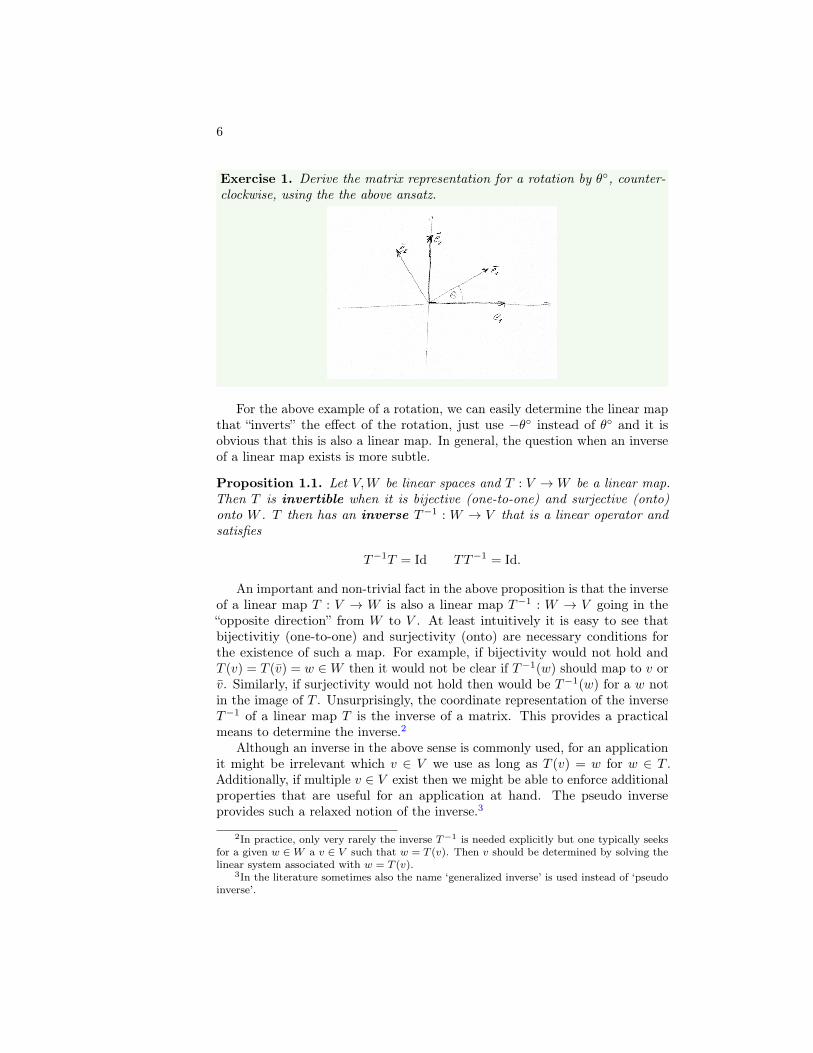
Exercise 1. Derive the matrix representation for a rotation by θ, counter-clockwise, using the the above ansatz.
For the above example of a rotation, we can easily determine the linear mapthat “inverts” the effect of the rotation, just use −θ instead of θ and it isobvious that this is also a linear map. In general, the question when an inverseof a linear map exists is more subtle.
Proposition 1.1. Let V,W be linear spaces and T : V →W be a linear map.Then T is invertible when it is bijective (one-to-one) and surjective (onto)onto W . T then has an inverse T−1 : W → V that is a linear operator andsatisfies
T−1T = Id TT−1 = Id.
An important and non-trivial fact in the above proposition is that the inverseof a linear map T : V → W is also a linear map T−1 : W → V going in the“opposite direction” from W to V . At least intuitively it is easy to see thatbijectivitiy (one-to-one) and surjectivity (onto) are necessary conditions forthe existence of such a map. For example, if bijectivity would not hold andT (v) = T (v) = w ∈W then it would not be clear if T−1(w) should map to v orv. Similarly, if surjectivity would not hold then would be T−1(w) for a w notin the image of T . Unsurprisingly, the coordinate representation of the inverseT−1 of a linear map T is the inverse of a matrix. This provides a practicalmeans to determine the inverse.2
Although an inverse in the above sense is commonly used, for an applicationit might be irrelevant which v ∈ V we use as long as T (v) = w for w ∈ T .Additionally, if multiple v ∈ V exist then we might be able to enforce additionalproperties that are useful for an application at hand. The pseudo inverseprovides such a relaxed notion of the inverse.3
2In practice, only very rarely the inverse T−1 is needed explicitly but one typically seeksfor a given w ∈W a v ∈ V such that w = T (v). Then v should be determined by solving thelinear system associated with w = T (v).
3In the literature sometimes also the name ‘generalized inverse’ is used instead of ‘pseudoinverse’.
7
Definition 1.5. Let V,W be linear spaces and T : V →W be a linear map. Aleft pseudo inverse T−1
L of T is a linear map T−1L : W → V such that
T−1L T = Id.
A right pseudo inverse T−1R of T is a linear map T−1
R : W → V such that
TT−1R = Id.
When T has an inverse in the sense of Proposition 1.1 then the left and rightpseudo inverse coincide and they are equal to the inverse T−1.
Note that in contrast to the inverse the pseudo inverse is in general notunique. For example two different right pseudo inverses T−1
R and T−1R can
yield v = T−1L (w) and v = T−1
L (w) and both are valid as long as T (T−1L (w)) =
T (T−1L (w)) = w.
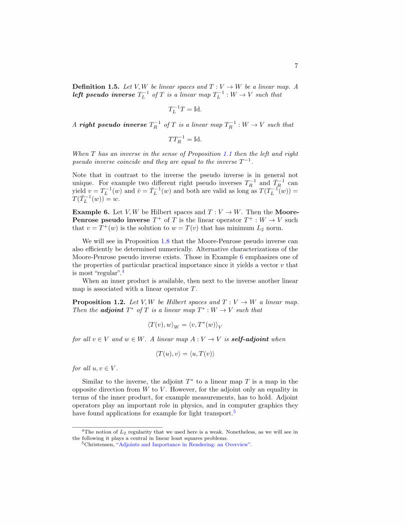
Example 6. Let V,W be Hilbert spaces and T : V →W . Then the Moore-Penrose pseudo inverse T+ of T is the linear operator T+ : W → V suchthat v = T+(w) is the solution to w = T (v) that has minimum L2 norm.
We will see in Proposition 1.8 that the Moore-Penrose pseudo inverse canalso efficiently be determined numerically. Alternative characterizations of theMoore-Penrose pseudo inverse exists. Those in Example 6 emphasizes one ofthe properties of particular practical importance since it yields a vector v thatis most “regular”.4
When an inner product is available, then next to the inverse another linearmap is associated with a linear operator T .
Proposition 1.2. Let V,W be Hilbert spaces and T : V → W a linear map.Then the adjoint T ∗ of T is a linear map T ∗ : W → V such that
〈T (v), w〉W = 〈v, T ∗(w)〉V
for all v ∈ V and w ∈W . A linear map A : V → V is self-adjoint when
〈T (u), v〉 = 〈u, T (v)〉
for all u, v ∈ V .
Similar to the inverse, the adjoint T ∗ to a linear map T is a map in theopposite direction from W to V . However, for the adjoint only an equality interms of the inner product, for example measurements, has to hold. Adjointoperators play an important role in physics, and in computer graphics theyhave found applications for example for light transport.5
4The notion of L2 regularity that we used here is a weak. Nonetheless, as we will see inthe following it plays a central in linear least squares problems.
5Christensen, “Adjoints and Importance in Rendering: an Overview”.
8
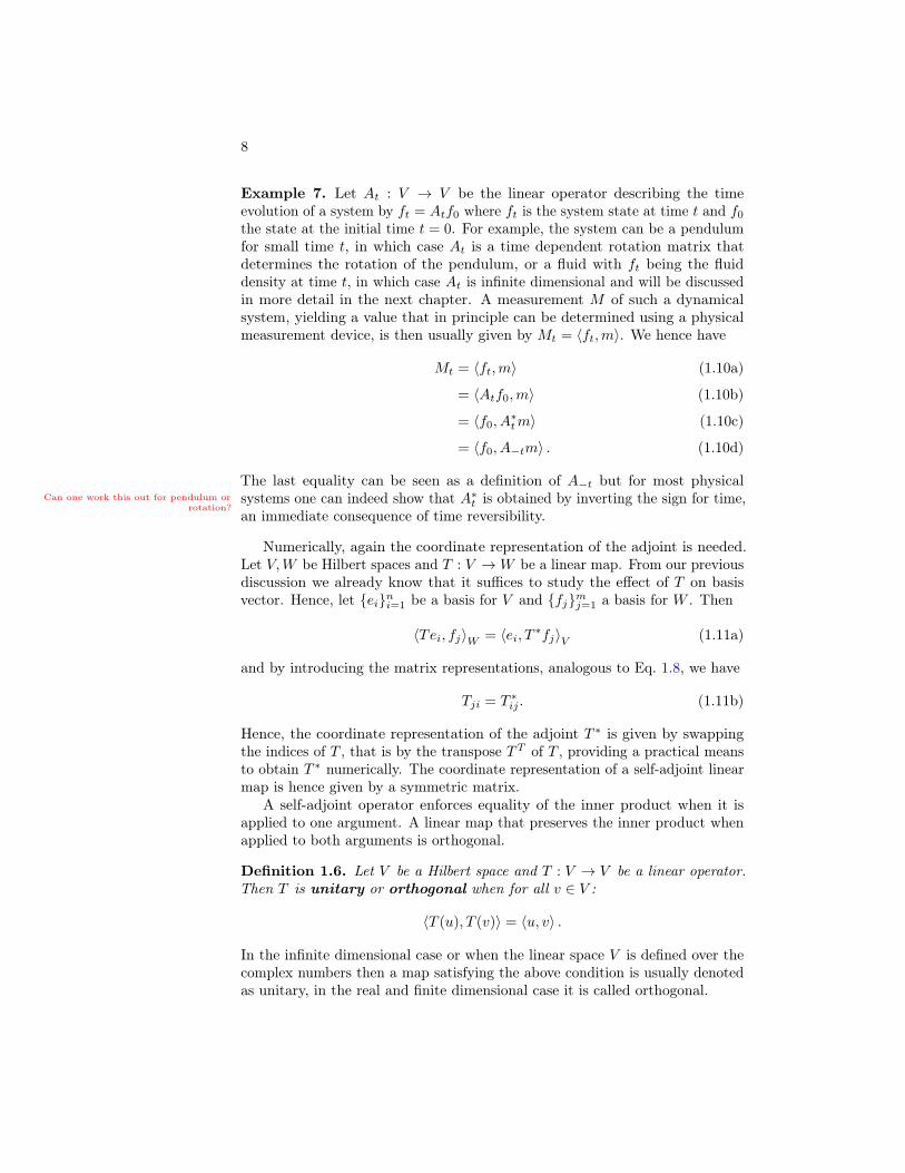
Example 7. Let At : V → V be the linear operator describing the timeevolution of a system by ft = Atf0 where ft is the system state at time t and f0
the state at the initial time t = 0. For example, the system can be a pendulumfor small time t, in which case At is a time dependent rotation matrix thatdetermines the rotation of the pendulum, or a fluid with ft being the fluiddensity at time t, in which case At is infinite dimensional and will be discussedin more detail in the next chapter. A measurement M of such a dynamicalsystem, yielding a value that in principle can be determined using a physicalmeasurement device, is then usually given by Mt = 〈ft,m〉. We hence have
Mt = 〈ft,m〉 (1.10a)
= 〈Atf0,m〉 (1.10b)
= 〈f0, A∗tm〉 (1.10c)
= 〈f0, A−tm〉 . (1.10d)
The last equality can be seen as a definition of A−t but for most physicalsystems one can indeed show that A∗t is obtained by inverting the sign for time,an immediate consequence of time reversibility.
Can one work this out for pendulum orrotation?
Numerically, again the coordinate representation of the adjoint is needed.Let V,W be Hilbert spaces and T : V →W be a linear map. From our previousdiscussion we already know that it suffices to study the effect of T on basisvector. Hence, let eini=1 be a basis for V and fjmj=1 a basis for W . Then
〈Tei, fj〉W = 〈ei, T ∗fj〉V (1.11a)
and by introducing the matrix representations, analogous to Eq. 1.8, we have
Tji = T ∗ij . (1.11b)
Hence, the coordinate representation of the adjoint T ∗ is given by swappingthe indices of T , that is by the transpose TT of T , providing a practical meansto obtain T ∗ numerically. The coordinate representation of a self-adjoint linearmap is hence given by a symmetric matrix.
A self-adjoint operator enforces equality of the inner product when it isapplied to one argument. A linear map that preserves the inner product whenapplied to both arguments is orthogonal.
Definition 1.6. Let V be a Hilbert space and T : V → V be a linear operator.Then T is unitary or orthogonal when for all v ∈ V :
〈T (u), T (v)〉 = 〈u, v〉 .
In the infinite dimensional case or when the linear space V is defined over thecomplex numbers then a map satisfying the above condition is usually denotedas unitary, in the real and finite dimensional case it is called orthogonal.
9
Proposition 1.3. Let V be a finite dimensional Hilbert space. The coordinaterepresentation of an orthogonal linear map T : V → V is an orthogonalmatrix T satisfying
T T−1 = T−1T = Id.
Exercise 2. Show that the above proposition holds.
We have by definition of an orthogonal operator for an orthonormal basiseini=1 for V that
〈T (ei), T (ej)〉 = 〈ei, ej〉 (1.12a)
and by the orthonormality of the basis this equals
〈T (ei), T (ej)〉 = δij . (1.12b)
Writing the operators and the inner product in their coordinate representationwe have
n∑a=1
(n∑b=1
Tab eib
)(n∑c=1
Tac ejc
)= δij (1.12c)
and taking the adjoint of Tab and reordering the summations yields
n∑b=1
n∑c=1
eib ejc
(n∑a=1
Tba Tac
)= δij . (1.12d)
Since the last equation has to hold for all tupled (i, j) we have to have
n∑a=1
Tab Tac = TT · T = Id. (1.13)
Since V is finite dimensional TT · T = Id also implies T · TT = Id.
Proposition 1.4. An orthogonal matrix T has rows and columns that areorthonormal as vectors. For example, for the columns it holds
n∑a=1
Tac Tbc = δab. (1.14)
Exercise 3. Show that the above proposition holds.
An alternative perspective on orthogonal matrices is as rotations. Indeed,we have both in R2 and R3 that rotation matrices, for example
R(θ) =
(cos θ − sin θsin θ cos θ
)(1.15)
10
are orthogonal by the Pythagorean trigonometric identity.6 The above definitionusing either the orthonormality of columns or that the inverse is given by thetranspose are those that work for arbitrary dimensions, whereas formulas interms of the rotation angles are only available in two or three dimensions. Wewill see yet another perspective on orthogonal matrices in the next section.
A classical example for linear maps, and one that is of considerable impor-tance in practice, are change-of-basis maps. In fact, their matrix representationare the bases matrices we already encountered in the foregoing. It might seemthat it does not make sense to abstractly talk about such maps without a coor-dinate representation but we will see that this is not the case in the followingin Sec. 1.5.2.
Proposition 1.5. Let V be a Hilbert space with orthonormal basis eini=1,and let fimi=1 be an arbitrary frame for V . Then the basis matrix Bei(fj)of fimi=1 with respect to eini=1 given by
Be(f) =
〈f1, e1〉 · · · 〈f1, e1〉...
. . ....
〈fm, en〉 · · · 〈fm, en〉
∈ Rm×n.
provides the change-of-basis from eini=1 to fimi=1 so that v(f)1
...v(f)m
= Be(f)
v(e)1
...v(e)n
where the v(e)i are the coefficients of v ∈ V with respect to eini=1 and thev(f)i are those with respect to fimi=1.
We have already derived part of this result before and the reader should recallhow the matrix B can be derived. Proposition 1.5 shows that the basis matrixprovides on the one hand the numerical representation of the basis, since everyrow is the basis expansion of one of the basis functions fi, and at the same timea way to determine the expansion function coefficients for the basis or frame.This viewpoint further strengthened by the next result.
Proposition 1.6. Under the assumptions of the foregoing proposition, thecolumns of a right pseudo inverse B−1
R contain the basis expansion of the dualframe functions fi with respect to eini=1 so that
v =
m∑i=1
⟨v, fi
⟩fi.
6By Euler’s theorem, which states that every rotation in R3 can be expressed as a rotationaround a suitably chosen axis, it suffices to consider the two-dimensional case.
11
Note that the role of the fi is fixed when the right pseudo inverse B−1R is used
to obtain them. When the fi are used for analysis to obtain the coefficients vi,that is
v =
m∑i=1
〈v, fi〉 fi (1.16)
then a left pseudo inverse B−1L has to be employed to obtain the fi. Also recall
from Proposition 1.1 that in the case B has a regular inverse then the pseudoinverse coincides with the inverse. This is the case when fimi=1 forms a basisand m = n and the fi are then the biorthogonal dual basis functions. Since thenB−1B = BB−1 = Id for a biorthogonal basis the primary and dual functionscan both be used for projection and reconstruction.
This concludes our discussion of the fundamental properties of linear opera-tors. Such operators will play a central role in all subsequent chapters.
Homework 3. Show that the space of linear maps T : V →W from a linearspace V to a linear space W has itself the structure of a vector space. Beginby developing the linear structure for the space of m× n matrices.
1.5.2 Eigen and Singular Value Decomposition
Operators and their representation as matrix are often abstract and unintuitive.The eigen and singular value decomposition provide important tools to analyzeand understand operators. Let us begin by recalling what we mean by aneigenvector and an eigenvalue.
Definition 1.7. Let V be a Hilbert space space and T : V → V a linear mapon V . An eigenvector v of T satisfies
Tv = λv
and λ is an eigenvalue of T .
Eigenvectors and eigenvalues are also only defined for a linear map T : V → Vthat maps a linear space into itself. A generalization that is defined also whenT : W → V is the singular value decomposition that will be introduced atthe end of the section. Note that v does not have to be unique, even whenwe identify linear dependent vectors, and then a nontrivial subspace of V isassociated with the eigenvalue λ. Typically one assumes that eigenvectors arenormalized, that is ‖v‖ = 1, and then the only degree of freedom that is left isthe sign of the eigenvalue, that is we have (λ, v) and (−λ,−v) both representthe same eigenvalue-eigenvector pair.
Example 8. Let R be a rotation in R3. Then R has an eigenvalue λ = 1 sothat Rv = v. The eigenvector v that is preserved under R is the rotation axis
12
and we see that any rotation in R3 can be considered as a two-dimensionalrotation around a fixed axis. The result is known as Euler’s theorem.7
Draw figure
Example 9. In Definition 1.4 we introduced the kernel of a linear map. ByDefinition 1.7 we can characterize the kernel of a map T as the subspace of Vassociated with the eigenvalue λ = 0. This characterization is computationallyimportant since it enables to numerically determine the kernel of a linear mapin its coordinate representation.8 By Theorem 1.3 below, the eigenvectorsassociated with kernel thereby have to be chosen such that they are orthogonalto all remaining eigenvectors. In the finite dimensional case, this uniquely fixesthe eigenvectors that span the kernel.
As a concrete example let us consider the projection Px onto the x-axis inR2:
Draw figure for x-projection in R2.The matrix representation of Px is given by
Px =
(1 00 0
)(1.17)
and it is immediately apparent that the eigenvalues and eigenvectors are:
λ1 = 1 v1 = (1.0, 0.0)T
λ2 = 0 v2 = (0.0, 1.0)T. (1.18)
It holds for arbitrary projection operators that the eigenvalues are all eitherzero or one. The example of Px is a special case of a diagonal matrix which wewill consider again in Example 10.
Theorem 1.3 (Spectral Theorem for Self-Adjoint Operators). Let H be aHilbert space and T a compact, self-adjoint operator. Then the eigenvectors viof T provide an orthonormal basis for V and the eigenvalues of T are real.
Obviously, the above result also holds in the finite dimensional case. T is thenself-adjoint when it is symmetric and compactness is always satisfied. WhenT is not symmetric one will obtain complex-valued eigenvalues. In the infinitedimensional case various generalizations beyond the case of compact operatorsexist but since their treatment would require considerable additional technicalmachinery we restrict ourselves to the above result and exclusively consider thefinite dimensional case in the following. However, we will consider a specialinstance of the infinite dimensional case in the next chapter.
7For a proof see for example (Marsden and Ratiu, Introduction to Mechanics and Sym-metry: A Basic Exposition of Classical Mechanical Systems, Chapter 9.2).
8Strictly speaking, due to the limited precision of computers, only the numerical kernelcan be determined, say up to floating point precision.
13
Example 10. Let D be a diagonal matrix, that is a square matrix satisfying
D =
d1 0 · · ·0 d2 0 · · ·
. . . . . . . . .· · · 0 dn−1 0
· · · 0 dn
(1.19)
Then the kth eigenvalues and the associated eigenvector are given by
λk = dk vk = (0, · · · , 1, · · · , 0)T (1.20)
where the kth element of vk is non-zero.
Example 11. Let C be a circulant matrix, that is a square matrix satisfying
C =
c0 cn−1 · · · c2 c1c1 c0 · · · c3 c2...
. . ....
cn−2 cn−3 · · · c0 cn−1
cn−1 cn−2 · · · c1 c0
(1.21)
The eigenvalues and eigenvectors of C are complex since C is not symmetric.Through the special structure of C the eigenvectors and eigenvalues have ananalytic form. The eigenvectors are given by
vk = (1, ωk, ω2k, · · · , ωn−1
k ) , ωk = e2πik/n (1.22)
where i is the imaginary unit with i =√−1. The corresponding eigenvalues are
λk = c0 + cn−1ωk + · · ·+ c1ωn−1k . (1.23)
The vi are related to discrete Fourier basis functions, which arise for examplein the discrete Fourier transform. Their connection to the harmonics can beseen by Euler’s formula eiθ = cos θ + i sin θ so that
ωk = e2πik/n = cos (2πi k/n) + i sin (2πi k/n) (1.24a)
= cos (2πi λk) + i sin (2πi λk) (1.24b)
with the λk being equidistant samples on [0, 1]. Hence, the vk are the discreteFourier transform functions sampled at λk.
figureThis also implies that the vk are orthogonal. In the following chapter, we
will also see the infinite dimensional analogue of this example.
Except for special cases, we have to compute the eigenvalues and eigenvectorsnumerically using tools from numerical linear algebra,9 a subject that goesbeyond the present notes.
9For an introduction see for example (Golub and Van Loan, Matrix Computations).
14
Remark 1. An alternative perspective on the eigen decomposition of a matrixis to consider it as a factorization of the form
A = USUT (1.25a)
where U is the orthogonal matrix whose columns are the eigenvectors and S isdiagonal with the eigenvalues being the nonzero entries, that is
A =
v1 · · · vn
λ1
λ2 0. . .
0 λn−1
λn
v1
...vn
. (1.25b)
Since U is orthogonal its columns form an orthonormal basis, cf. Proposition 1.4,and UT is the change of basis matrix into this basis. By Eq. 1.25a, the actionA(v) of A applied to v can also be understood as first transforming v usingUT into a basis where A is diagonal, then applying A in its diagonalized formby S, and then transforming back to the original basis so that the result of(USUT )(v) indeed equals A(v). The eigen decomposition is hence also oftendenoted as the diagonalization of an operator.
Exercise 4. Consider the linear map
A =
(1.6250 0.64950.6495 0.8750
). (1.26)
Determine and interpret its eigen decomposition.
Since A is symmetric it has a real eigen decomposition given by
A = USUT =
(0.87 −0.500.50 0.87
)(2.0 0.00.0 0.5
)(0.87 0.50−0.50 0.87
). (1.27)
By construction, the change of basis matrix U is given by
U = R(30) =
(cos θ − sin θsin θ cos θ
). (1.28)
Hence, A(v) corresponds to a change of basis to a coordinate basis that isrotated by 30 with respect to the standard basis for R2, then a scaling in therotated coordinate system, and finally a change of basis back to the standardbasis for R2.
figure: draw the effect of A with a sketch of the rotated coordinate system
The eigen decomposition exists only when T : V → V is a linear map froma space onto itself. A generalization that is well defined also when T : V →Wis the singular value decomposition.
15
Definition 1.8. Let V,W be finite linear spaces and T : V → W be a linearmap. Then u ∈ W is a left singular vector and v ∈ V a right singularvector of T when
T v = σ u
and σ is the singular value associated to (u, v).
The singular value decomposition also exists in the infinite dimensional casebut we will not consider it here.10 The importance of the singular vectors andvalues stems from the following proposition.
Proposition 1.7. Let V,W be Hilbert spaces of dimension n andm, respectively,and let T : V → W be a linear map. In matrix form the singular valuedecomposition is given by
T = UΣV T .
where the columns of U are formed by left singular vectors ui and the columns ofV by right singular vectors vi, and Σ is a quasi-diagonal matrix whose nonzeroentries are the singular values. Moreover, the left singular vectors uini=1
form an orthonormal basis for W and the right singular vectors vimi=1 anorthonormal basis for V .
It is customary to order the singular values in non-decreasing order so thatσi ≥ σi+1 and we will follow this convention in the following. It follows fromthe definition that only for T and m× n matrix there are at most min(m,n)nonzero singular values.
Remark 2. For a rectangular matrix T ∈ Rm×n the matrix Σ is only quasi-diagonal. For m < n this means
Σ =
σ1 · · · 0 0 · · · 0...
. . ....
.... . .
...0 · · · σm 0 · · · 0
(1.29)
and the matrix has the form of the m×m identity matrix with an m× (n−m)block that is a zero matrix adjoining on the right. Conversely, when m > nthen Σ has the form
Σ =
σ1 · · · 0...
. . ....
0 · · · σn0 · · · 0...
. . ....
0 · · · 0
. (1.30)
10For the infinite dimensional case see for example (Stakgold and Holst, Green’s Functionsand Boundary Value Problems) or Lax (Lax, Functional Analysis, Chapter 30).
16
Remark 3. The eigen decomposition is a special case of the singular valuedecomposition. Because of the significance for quantum mechanics, the eigendecomposition has been developed earlier and in more detail.
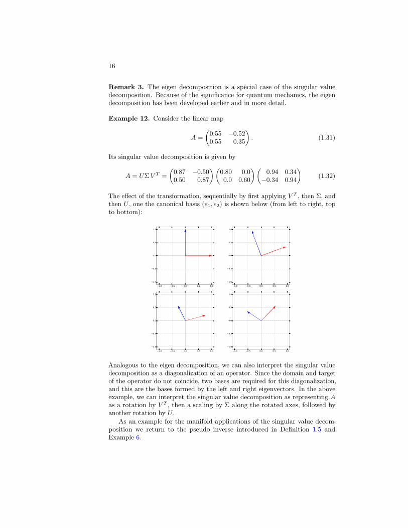
Example 12. Consider the linear map
A =
(0.55 −0.520.55 0.35
). (1.31)
Its singular value decomposition is given by
A = UΣV T =
(0.87 −0.500.50 0.87
)(0.80 0.00.0 0.60
)(0.94 0.34−0.34 0.94
)(1.32)
The effect of the transformation, sequentially by first applying V T , then Σ, andthen U , one the canonical basis (e1, e2) is shown below (from left to right, topto bottom):
1.0 0.5 0.0 0.5 1.0
1.0
0.5
0.0
0.5
1.0
1.0 0.5 0.0 0.5 1.0
1.0
0.5
0.0
0.5
1.0
1.0 0.5 0.0 0.5 1.0
1.0
0.5
0.0
0.5
1.0
1.0 0.5 0.0 0.5 1.0
1.0
0.5
0.0
0.5
1.0
Analogous to the eigen decomposition, we can also interpret the singular valuedecomposition as a diagonalization of an operator. Since the domain and targetof the operator do not coincide, two bases are required for this diagonalization,and this are the bases formed by the left and right eigenvectors. In the aboveexample, we can interpret the singular value decomposition as representing Aas a rotation by V T , then a scaling by Σ along the rotated axes, followed byanother rotation by U .
As an example for the manifold applications of the singular value decom-position we return to the pseudo inverse introduced in Definition 1.5 andExample 6.
17
Proposition 1.8. Let T : Rn → Rm be a linear map with singular valuedecomposition T = UΣV T . Then the Moore-Penrose pseudo-inverse T+ of isgiven by
T+ = V Σ+ UT (1.33)
where Σ+ is the diagonal matrix whose ith diagonal element is given by 1/σi,that is Σ+ is obtained by inverting the diagonal entries.
The above proposition provides a practical means to compute the Moore-Penrose pseudo inverse. Note that as a special case one also obtains meansto compute the inverse. This technique is however more expensive than usingstate-of-the-art numerical techniques.11
Exercise 5. Show that the inverse of a square diagonal matrix
D =
d1 · · · 0...
. . ....
0 · · · dn
(1.34)
is given by
D−1 =
1/d1 · · · 0...
. . ....
0 · · · 1/dn
. (1.35)
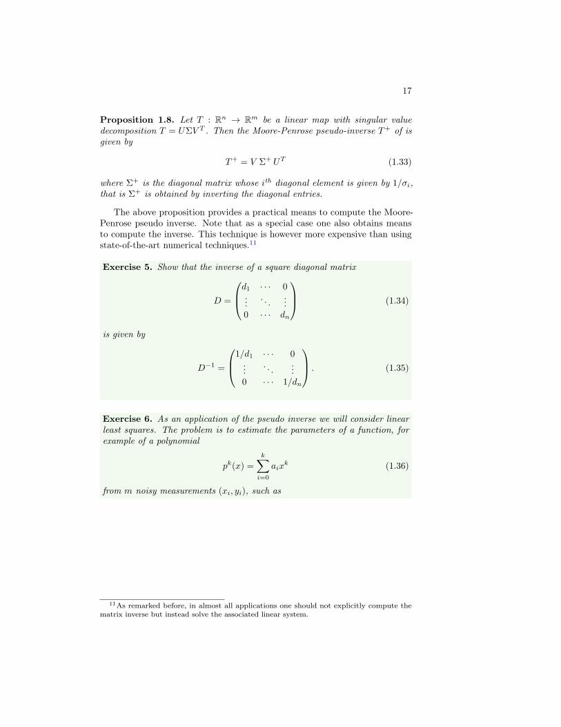
Exercise 6. As an application of the pseudo inverse we will consider linearleast squares. The problem is to estimate the parameters of a function, forexample of a polynomial
pk(x) =
k∑i=0
aixk (1.36)
from m noisy measurements (xi, yi), such as
11As remarked before, in almost all applications one should not explicitly compute thematrix inverse but instead solve the associated linear system.

18
1.0 0.5 0.0 0.5 1.01.2
1.0
0.8
0.6
0.4
0.2
0.0
0.2
0.4
For the above data a reasonable model seems to be a first order polynomial,that is p(x) = a0 + a1 x. However, the data clearly does not perfectly lie on aline, since the measurements were contaminated with noise, and we also havefar too many measurements to directly determine the two parameters a0 anda1. Clearly, we would like to use the fact that we have m >> 2 measurementsto make our estimate robust and average out the contribution of the noise.
The measurements should all satisfy the linear equation. Hence we have
y1 = a0 + a1x1
y2 = a0 + a1x2
· · ·
ym = a0 + a1xm
Since the a0,a1 are identical for all equations we can write equivalently asmatrix-vector equation
y =
y1
...ym
=
1.0 x1
......
1.0 xm
(a0
a1
)= Xa. (1.37)
The above equation is an overdetermined linear system. Hence, a solutioncan be determined using a pseudo inverse as a = P−1
L y. But which pseudoinverse should be used? One can show that the Moore-Penrose, which can bedetermined using the singular value decomposition, yields the solution a thatminimizes the quadratic error12
E(a0, a1) =
n∑i=1
‖yi − pa0,a1(xi)‖2 . (1.38)
One can show that the minimizer can also be determined without the pseudoinverse by solving the normal equation
XT y = XTXa. (1.39)
19
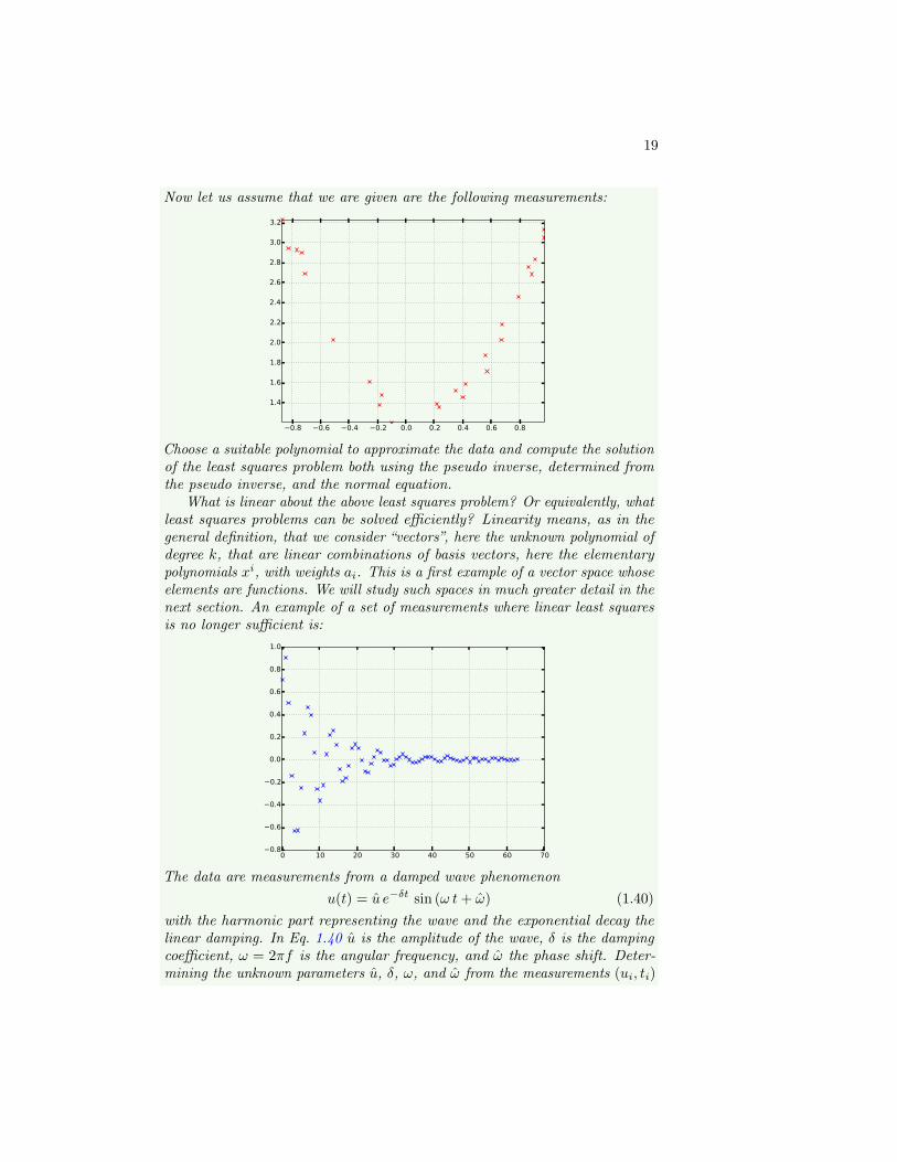
Now let us assume that we are given are the following measurements:
0.8 0.6 0.4 0.2 0.0 0.2 0.4 0.6 0.8
1.4
1.6
1.8
2.0
2.2
2.4
2.6
2.8
3.0
3.2
Choose a suitable polynomial to approximate the data and compute the solutionof the least squares problem both using the pseudo inverse, determined fromthe pseudo inverse, and the normal equation.
What is linear about the above least squares problem? Or equivalently, whatleast squares problems can be solved efficiently? Linearity means, as in thegeneral definition, that we consider “vectors”, here the unknown polynomial ofdegree k, that are linear combinations of basis vectors, here the elementarypolynomials xi, with weights ai. This is a first example of a vector space whoseelements are functions. We will study such spaces in much greater detail in thenext section. An example of a set of measurements where linear least squaresis no longer sufficient is:
0 10 20 30 40 50 60 700.8
0.6
0.4
0.2
0.0
0.2
0.4
0.6
0.8
1.0
The data are measurements from a damped wave phenomenonu(t) = u e−δt sin (ω t+ ω) (1.40)
with the harmonic part representing the wave and the exponential decay thelinear damping. In Eq. 1.40 u is the amplitude of the wave, δ is the dampingcoefficient, ω = 2πf is the angular frequency, and ω the phase shift. Deter-mining the unknown parameters u, δ, ω, and ω from the measurements (ui, ti)

20
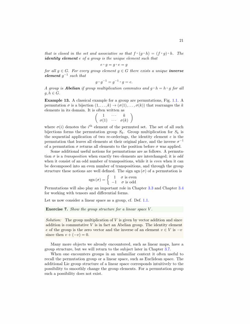
Figure 1.1: A group can be considered as the set of possible transformations of a setsuch as the possible arrangements, or permutations, of “color tiles” on a 2× 2 panel.
such that the quadratic error
E(u, δ, ω, ω) =
m∑i=1
‖ui − uu,δ,ω,ω(ti)‖2 (1.41)
is minimized is a nonlinear problem since parameters appear both in theexponent of the exponential and inside the sine term. Such a nonlinear leastsquares problem requires iterative methods such as the Gauss-Newton algorithmfor its solution.
Solution: See linear_least_squares.py.
Homework 4. Using the singular value decomposition describe the three casesthat exist for the pseudo inverse with respect to the relationship of m and nfor an m× n matrix.
1.6 Linear Spaces as Groups
Groups and their continuous extension, known as Lie groups, are subjects wewill only scratch on in this course. A classical example for Lie groups, andone of the original templates for the concept, are linear spaces. Lie groups willbe discussed in Chapter 3.7 but we will already introduce the regular groupstructures of linear spaces at this point.
Definition 1.9. A group G is a set with a binary group multiplication
g h = gh : G×G→ G, g, h ∈ G
21
that is closed in the set and associative so that f (g h) = (f g) h. Theidentity element e of a group is the unique element such that
e g = g e = g
for all g ∈ G. For every group element g ∈ G there exists a unique inverseelement g−1 such that
g g−1 = g−1 g = e.
A group is Abelian if group multiplication commutes and g h = h g for allg, h ∈ G.
Example 13. A classical example for a group are permutations, Fig. 1.1. Apermutation σ is a bijection (1, . . . , k)→ (σ(1), . . . , σ(k)) that rearranges the kelements in its domain. It is often written as(
1 · · · kσ(1) · · · σ(k)
)where σ(i) denotes the ith element of the permuted set. The set of all suchbijections forms the permutation group Sk. Group multiplication for Sk isthe sequential application of two re-orderings, the identity element e is thepermutation that leaves all elements at their original place, and the inverse σ−1
of a permutation σ returns all elements to the position before σ was applied.Some additional useful notions for permutations are as follows. A permuta-
tion σ is a transposition when exactly two elements are interchanged; it is oddwhen it consist of an odd number of transpositions, while it is even when it canbe decomposed into an even number of transpositions, and through the groupstructure these notions are well defined. The sign sgn (σ) of a permutation is
sgn (σ) =
1 σ is even−1 σ is odd
Permutations will also play an important role in Chapter 3.3 and Chapter 3.4for working with tensors and differential forms.
Let us now consider a linear space as a group, cf. Def. 1.1.
Exercise 7. Show the group structure for a linear space V .
Solution: The group multiplication of V is given by vector addition and sinceaddition is commutative V is in fact an Abelian group. The identity elemente of the group is the zero vector and the inverse of an element v ∈ V is −vsince then v + (−v) = 0.
Many more objects we already encountered, such as linear maps, have agroup structure, but we will return to the subject later in Chapter 3.7.
When one encounters groups in an unfamiliar context it often useful torecall the permutation group or a linear space, such as Euclidean space. Theadditional Lie group structure of a linear space corresponds intuitively to thepossibility to smoothly change the group elements. For a permutation groupsuch a possibility does not exist.
22
1.7 Affine Spaces
In the foregoing, we always used R2, or more generally Euclidean space, asan example of a vector space. However, this model can only represent vectorsstarting at the origin and not point and the translation of points using vectors.A model for Euclidean space that incorporates both points and vectors is anaffine space. Another model, which subsumes the previous ones, follows inChapter 3.
Definition 1.10. An affine space is a set A together with a vector space Vand a map
t : V ×A→ A : v + a→ b
for a, b ∈ A and v, w ∈ V , that satisfies
i) identity: 0 + a = a, ∀a ∈ A;
ii) associativity: (v + w) + a = v + (w + a);
iii) uniqueness: v + a = b is a bijection .
The last property of the translation map ‘+’ ensures the existence of welldefined inverse which is denoted by ‘−’ and which allows to combine twoelements of A to form a vector, that is v = a− b. An affine space is sometimesdenoted as a vector space where one forgot the origin since vectors are no longerrequired to be based on the origin but can start from any point in the plane.
Example 14. Euclidean space E2 is the two dimensional plane together withthe vector space R2.
It is common to use Rn for both the vector space and the affine space En.
Remark 4. The name ‘affine’ comes from affine combinations of the form
λa+ (1− λ)b = o+ λ(a− o) + (1− λ)(b− o) (1.42)
for a, b ∈ A and λ ∈ R. In an affine space only such combinations are indepen-dent of the (in an affine space arbitrary) origin o.
Exercise 8. For the following example, show that only for affine combinationsand not general linear combinations the addition of two points is independentof the origin in R2. With respect to the usual origin o = (0.0, 0.0), let a =(1.0, 1.5), b = (−1.4, 1.2) and furthermore let a second origin be o = (1.0, 1.0).Also we use λ = 0.75, β = 0.5.
23
Solution: For the affine combination with the origin being o we have
λa+ (1− λ)b =
(0.751.125
)+
(−0.35
0.3
)=
(0.4
1.425
). (1.43a)
Moving the origin to o = (1.0, 1.0) we have a = (0.0, 0.5), b = (−2.4, 0.2) .Then
λa+ (1− λ)b =
(0.750.375
)+
(−0.60.05
)=
(−0.60.425
). (1.43b)
And translating the result back from o to o we see that the affine combinationis indeed independent of the origin. In contrast,
λa+ βb =
(0.0
1.125
)+
(−0.7
0.6
)=
(0.051.725
)(1.44a)
and
λa+ βb =
(0.0
0.375
)+
(−1.2
0.1
)=
(−1.20.475
). (1.44b)
Translated back to the origin we thus have (0.2, 1.475) which does not equalthe result for o.
A central property of affine spaces is that the linear addition of a point bya vector yields again a point in the space. Manifolds, which will be studiedin Chapter 3, are spaces that are not closed under linear addition but wherenonlinear curves are needed to connect points in the space.
Remark 5. An affine space is an example of a group action, here the action ofa linear space considered as a group, on another space or set. We will studythis idea in more detail in Chapter 3.7.
TODO: Affine transformations, in affine space translations are defined,which is not case in a vector space; to represent it as a linear map one needshomogeneous coordinates, that is translations are not linear maps with respectto the vector space structure.
1.8 Further Reading
The abstract perspective on linear spaces is discussed for example by Lax.13Classical texts on matrix theory are those by Horn and Johnson14 and by Goluband van Loan.15
13Lax, Linear Algebra and Its Applications.14Horn and Johnson, Matrix Analysis.15Golub and Van Loan, Matrix Computations.

Chapter 2
Signal Processing andApplied Functional Analysis
In this section, we will study one of the most important class of examples forlinear spaces: linear spaces whose elements are continuous functions, so calledfunction spaces. Elements in function spaces that correspond to a quantityor phenomenon in the real world are often called “signals", in particular inengineering and the sciences. In computer graphics, signal processing andapplied functional analysis play important roles for example in rendering,1 forthe representation of signals and curves,2 and for mesh processing.3
2.1 Functions as Vectors in a Linear Space
In this chapter, we will consider spaces of functions. Hence, we will begin bymaking precise what we mean by a function.
Definition 2.1. Let X be a set. A function is a map
f : X → R
into the real numbers R.
1For example in precomputed radiance transfer, cf. (Lehtinen, “A Framework for Precom-puted and Captured Light Transport”; Ramamoorthi, “Precomputation-Based Rendering”),for radiosity, e.g. (Zatz, “Galerkin Radiosity: A Higher Order Solution Method for Global Illu-mination”; Gortler, Schröder, Cohen, and Hanrahan, “Wavelet Radiosity”; Schröder, Gortler,Cohen, and Hanrahan, “Wavelet Projections for Radiosity”), or for the representation andinterpolation of light intensity, e.g. (Lehtinen, Zwicker, Turquin, Kontkanen, Durand, Sillion,and Aila, “A Meshless Hierarchical Representation for Light Transport”; Mitchell, “SpectrallyOptimal Sampling for Distribution Ray Tracing”)
2For example, (Schröder and Sweldens, “Spherical Wavelets: Efficiently RepresentingFunctions on the Sphere”; Schröder and Sweldens, “Spherical Wavelets: Texture Processing”;Finkelstein and Salesin, “Multiresolution Curves”).
3For example (Taubin, “A Signal Processing Approach to Fair Surface Design”; Öztireli,Alexa, and Gross, “Spectral Sampling of Manifolds”; Sorkine, “Laplacian Mesh Processing”).
25
26
−1 −0.8 −0.6 −0.4 −0.2 0 0.2 0.4 0.6 0.8 1−2
−1
0
1
2
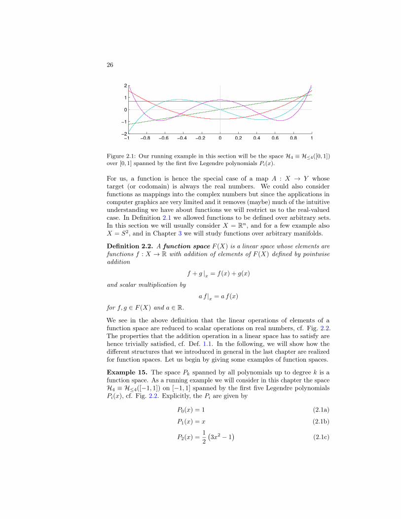
Figure 2.1: Our running example in this section will be the space H4 ≡ H≤4([0, 1])over [0, 1] spanned by the first five Legendre polynomials Pi(x).
For us, a function is hence the special case of a map A : X → Y whosetarget (or codomain) is always the real numbers. We could also considerfunctions as mappings into the complex numbers but since the applications incomputer graphics are very limited and it removes (maybe) much of the intuitiveunderstanding we have about functions we will restrict us to the real-valuedcase. In Definition 2.1 we allowed functions to be defined over arbitrary sets.In this section we will usually consider X = Rn, and for a few example alsoX = S2, and in Chapter 3 we will study functions over arbitrary manifolds.
Definition 2.2. A function space F (X) is a linear space whose elements arefunctions f : X → R with addition of elements of F (X) defined by pointwiseaddition
f + g |x = f(x) + g(x)
and scalar multiplication by
a f |x = a f(x)
for f, g ∈ F (X) and a ∈ R.
We see in the above definition that the linear operations of elements of afunction space are reduced to scalar operations on real numbers, cf. Fig. 2.2.The properties that the addition operation in a linear space has to satisfy arehence trivially satisfied, cf. Def. 1.1. In the following, we will show how thedifferent structures that we introduced in general in the last chapter are realizedfor function spaces. Let us begin by giving some examples of function spaces.
Example 15. The space Pk spanned by all polynomials up to degree k is afunction space. As a running example we will consider in this chapter the spaceH4 ≡ H≤4([−1, 1]) on [−1, 1] spanned by the first five Legendre polynomialsPi(x), cf. Fig. 2.2. Explicitly, the Pi are given by
P0(x) = 1 (2.1a)
P1(x) = x (2.1b)
P2(x) =1
2
(3x2 − 1
)(2.1c)
27
−1 −0.8 −0.6 −0.4 −0.2 0 0.2 0.4 0.6 0.8 1−2
−1
0
1
2
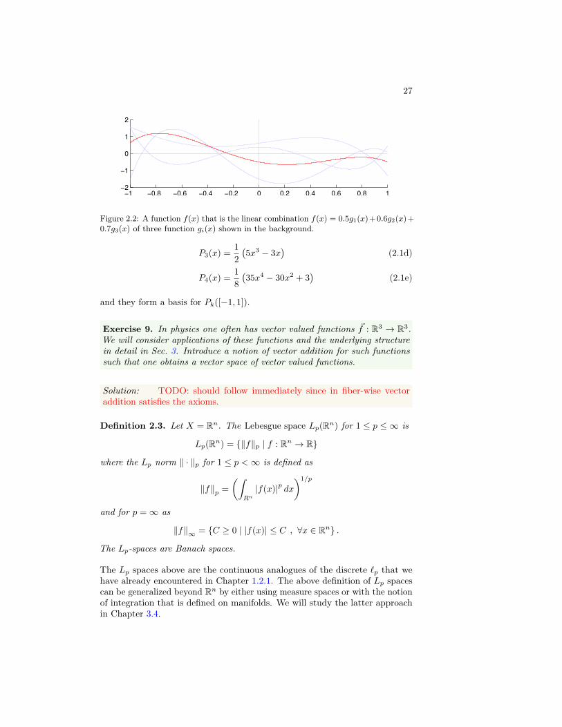
Figure 2.2: A function f(x) that is the linear combination f(x) = 0.5g1(x)+0.6g2(x)+0.7g3(x) of three function gi(x) shown in the background.
P3(x) =1
2
(5x3 − 3x
)(2.1d)
P4(x) =1
8
(35x4 − 30x2 + 3
)(2.1e)
and they form a basis for Pk([−1, 1]).
Exercise 9. In physics one often has vector valued functions ~f : R3 → R3.We will consider applications of these functions and the underlying structurein detail in Sec. 3. Introduce a notion of vector addition for such functionssuch that one obtains a vector space of vector valued functions.
Solution: TODO: should follow immediately since in fiber-wise vectoraddition satisfies the axioms.
Definition 2.3. Let X = Rn. The Lebesgue space Lp(Rn) for 1 ≤ p ≤ ∞ is
Lp(Rn) = ‖f‖p | f : Rn → R
where the Lp norm ‖ · ‖p for 1 ≤ p <∞ is defined as
‖f‖p =
(∫Rn|f(x)|p dx
)1/p
and for p =∞ as
‖f‖∞ = C ≥ 0 | |f(x)| ≤ C , ∀x ∈ Rn .
The Lp-spaces are Banach spaces.
The Lp spaces above are the continuous analogues of the discrete `p that wehave already encountered in Chapter 1.2.1. The above definition of Lp spacescan be generalized beyond Rn by either using measure spaces or with the notionof integration that is defined on manifolds. We will study the latter approachin Chapter 3.4.
28
Remark 6. For us, the Lp-spaces themselves are typically not of particularinterest. The functions of interest will usually be in all reasonable functionspaces, which, as we will see in the following, is a consequence of our restriction tofinite computations. It often also follows from modelling real world phenomena.The more important question for us is what does the Lp norms, or other normswe can consider, measure and do they represent the quantity or behaviour ofinterest to us. The norms most commonly used thereby are the L1, L2, and L∞norm. Compared to the L1 norm, the L2 norm is more sensitive to regions ofextreme values, since squaring amplifies these, but less sensitive to regions withsmall values, since squaring further diminishes their contribution in the norm.Obviously, which norm is most appropriate will depend on the application.
Definition 2.4. For X = Rn, the Sobolev space W k,p(Rn) for integers k ≥ 0and 1 ≤ p <∞ is the space
W k,p(X) = f ∈ Lp(X) | (Dαf) ∈ Lp(X) , ∀|α| ≤ k . (2.3)
Hence, for f to be in a Sobolev space all mixed derivatives Dα whose totalorder |α| is at most k have to lie in the Lebesgue space Lp(X), where α is amulti-index. When suitably completed, the Sobolev space W k,p forms a Banachspace whose norm is given by
‖f‖k,p =
∑|α|≤k
(‖Dαf‖p
)p1/p
(2.4)
where the summation is over all mixed derivatives of at most order k. Forp = ∞ Sobolev spaces are defined analogously to the corresponding Lebesguespaces.
In contrast to Lp spaces, the norm on Sobolev spaces also takes the derivativeinto account. It should then come at no surprise that Sobolev spaces playan important role in the theory of partial differential equations. As a lastexample for a Banach we consider another space that imposes a constraint onthe derivative, and hence how wildly a function can vary.
Example 16. Let X = R. The variation V ba (f) of a function f : R→ R is
V ba (f) =
∫ b
a
|f ′(x)| dx. (2.5)
The space of functions with bounded variation BV([a, b]) is hence defined as
BV([a, b]) =f ∈ L1([a, b]) | V ba (f) <∞
(2.6)
and it is a linear subspace of L1([a, b]). Moreover, with the norm
‖f‖BV = ‖f‖1 + V ba (f) (2.7)
the space BV([a, b]) is a Banach space. In higher dimensions and over morecomplex domains, the space of functions of bounded variation can be definedusing distributional derivatives. It should be noted that the space of functionsof bounded variation is not separable.
29
The space BV ([a, b]) is used for example in integration theory and we willencounter it again in Chapter 2.4.4. As in the general case, the function spacesthat are most useful are Hilbert spaces where an inner product is available.Recall that the Riesz representation theorem then enables to identify functionalsα ∈ H on the space, which map elements to real numbers and can be interpretedas general measurements, to functions f ∈ H in the space with the action beingrealized through the inner product
α(f) = 〈gα, f〉 . (2.8)
As in the discrete case, the space L2(Rn) is also in the case of function spaces aHilbert space.
Example 17. The Lebesgue space L2(Rn), cf. Example 2.3, is a Hilbert spacewith inner product
〈f, g〉 =
∫Rn
f(x) g(x) dx. (2.9)
The L2-inner product is by far the most common inner product encounteredfor function spaces and unless mentioned otherwise we will in the followingalways assume this inner product for function spaces.
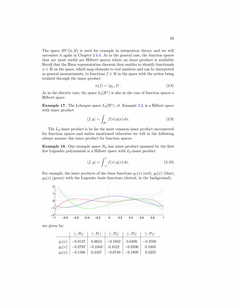
Example 18. Our example space H4 has inner product spanned by the firstfive Legendre polynomials is a Hilbert space with L2-inner product
〈f, g〉 =
∫ 1
−1
f(x) g(x) dx. (2.10)
For example, the inner products of the three functions g1(x) (red), g2(x) (blue),g3(x) (green) with the Legendre basis functions (dotted, in the background),
−1 −0.8 −0.6 −0.4 −0.2 0 0.2 0.4 0.6 0.8 1−2
−1
0
1
2
are given by:
〈·, P0〉 〈·, P1〉 〈·, P2〉 〈·, P3〉 〈·, P4〉
g1(x) −0.0137 0.0624 −0.1602 0.0498 −0.3708
g2(x) −0.2797 −0.2483 0.4522 −0.9506 0.1003
g3(x) −0.1566 0.2437 −0.6749 −0.1809 0.2355
30
Example 19. The Sobolev spaces W k,2(Rn) modelled on the Hilbert spacesL2(X) are Hilbert spaces, cf. Example 2.4, and the inner product for the spacesis given by
〈f, g〉 =∑|α|≤k
〈Dαf,Dαg〉 (2.11)
where the summation is over all multi-indices α that have at most order k, and〈 , 〉 is the L2-inner product of Example 17. The spaces area usually denoted asHilbert-Sobolev spaces Hs(X) = W s,2(X).
Exercise 10. Let us return to the example of vector valued functions ~f :R3 → R3. Introduce an inner product for such functions so that an L2 spacecan be defined.
Solution: We have an inner product at each point, by taking the innerproduct of vectors, and by replacing scalar multiplication by this vector-valuedmultiplication we obtain:⟨
~f,~g⟩
=
∫Rn
~f(x) · ~g(x) dx (2.12)
It needs to be shown that this inner product in fact satisfies all necessaryproperties, although this is at least reasonable since the pointwise inner productgiven by the dot product clearly satisfies them. The L2-space of vector valuedfunctions is then defined as usual as the space of all ~f that have finite L2
norm.
In the remainder of the section we will almost exclusively discuss L2-typeHilbert spaces. These are used most often in practice and their theory mostaccessible. A discussion of other Hilbert spaces, such as the Sobolev spaces H2,and Banach spaces would require a more specialized course.
2.2 Bases and Numerical Computations
Since function spaces are special instances of vector spaces, bases and framesprovide the principal means for performing numerical computations with con-tinuous functions. Sometimes this is thought to be paradoxical: how can oneperform computations with continuous functions on a discrete computer. Thekey is that a we want to perform computations on a finite machine. Hence, aslong as our function spaces are finite dimensional we will be able to performnumerical computations with them. However, the signals of interest will notalways be finite dimensional and hence we have to consider the question whichfinite dimensional space, or equivalently which basis, enables to approximatethe signals. Approximation of functions is a subject we will not be able todiscuss in detail but which we will at least introduce in Chapter 2.3.
31
Exercise 11. What does it mean for a function to be finite dimensional? Tryto develop a precise notion of the concept. Is it sufficient to consider onefunction?
Solution: Every function f is an element of a one-dimensional function space:the space spanned by f by af with a ∈ R. Hence, the notion of dimensionalityonly makes sense if we consider a family of functions. Typically, this are all thefunctions that can possibly and reasonably describe a phenomenon of interest.A useful example, and one that has been studied extensively in the literature,is the space of natural images.
2.2.1 Orthonormal Bases
• Repeat definition and most important properties of orthonormal bases.
• For finite dimensional Hilbert spaces H: isomorphism from H and Rn.
– Continuous function is equivalent to vector in Rn with the basisfunction coefficients providing the coordinates.
– Since we have an isomorphism, all operations in H are mapped to acorresponding operation in Rn.
∗ Addition.∗ Scalar multiplication.∗ ClassExercise: Inner product and L2 norm.∗ HomeworkExercise: Parseval’s identity.∗ How this applies to operators, which is called Galerkin projection,is discussed in Chapter 2.5.3.
– ClassExercise: Verify addition for random signals in H4.
– Remark: Fourier
∗ Fourier series vs. Fourier transform: compactness of domain canhave crucial difference.
∗ Fourier transform has a continuum of basis functions. Summa-tion has to be replaced by integration but all properties carryover by analogy.
∗ Historically, Fourier and polynomials (there’s a whole family oforthogonal polynomials) were the only bases, orthonormal ornot, that were in general considered as practical. It was onlybeginning in the 1980s that it was realized that many more basescould be construct and that these had many useful properties,like localization in space, that are not available with classicalbases.
32
Remark 7. We have seen that orthonormal bases provide a convenient andpowerful way to work numerically with continuous functions. However, torecover the result we often need the value of the function, at least pointwise forsome locations in the domain. This then requires to evaluate the basis functions.The requirement that the basis functions have to be evaluable accurately andefficiently yields a considerable constraint on the number of bases that arenumerically practical.
In our examples we employ Legendre polynomials. In principle, we couldevaluate the polynomials directly by implementing the formulas in Eq. 2.1 andfor H4 this is indeed a viable option. However, already for H10 this approachwould suffer from substantial inaccuracies due to the use of floating pointnumbers.4 Instead, the recurrence relation
(n+ 1)Pn+1(x) = (2n+ 1)xPn(x)− nPn−1(x). (2.13)
It is useful to keep in mind that even “elementary functions” such as sin(x) orlog (x) cannot be evaluated directly on a computer but that approximationalgorithms are employed that evaluate them up to machine precision (andfortunately these are implemented in hardware so that the computation takesonly a few processor cycles).
Remark 8. TODO: Tensor product spaces and based for them. Not compli-cated but has to be mentioned.
2.2.2 Biorthogonal Bases and Frames
• Repeat definition of biorthogonal bases.
• Frames as overcomplete bases:
• Practical motivation:
– Orthogonal bases are hard to construct and even if one can constructthem they are restrictive. Biorthogonal bases are much easier toconstruct and they are flexible enough so that one can incorporateother desirable properties (although it is typically not easy to enforcethese). What could be such properties? For example, the Legendrepolynomials are symmetric (more precisely symmetric and anti-symmetric) with respect to the y-axis. Such symmetries are oftendesirable since they avoid that one has directional bias in the basisrepresentation.
– Frames have redundancy which makes them robust against errorsand loss of information.
4The classical Numerical Recipes book writes on the subject: “Come the (computer)revolution, all persons found guilty of such criminal behavior [the evaluation of a polynomialby directly evaluating p(x) = a0 + a1x+ a2x2 + · · · ] will be summarily executed, and theirprograms won’t be!”, (Press, Teukolsky, Vetterling, and Flannery, Numerical Recipes in C:The Art of Scientific Computing, Chapter 5.3).
33
• Numerical representation:
– Basis matrix that is formed by basis expansion of ψi(x) with respectto some reference basis, that is each row of B contains the basisfunction coefficients for one function ψi(x).
– The reference basis is necessary for example so that we can evaluatethe functions.
– Dual basis is constructed by inverting the basis matrix. For overcom-plete frames the dual frame is not uniquely defined and numericallya pseudo inverse has to be employed to compute it; for example,we can employ the Moore-Penrose pseudo inverse that we discussedbefore and that can be computed using the SVD.
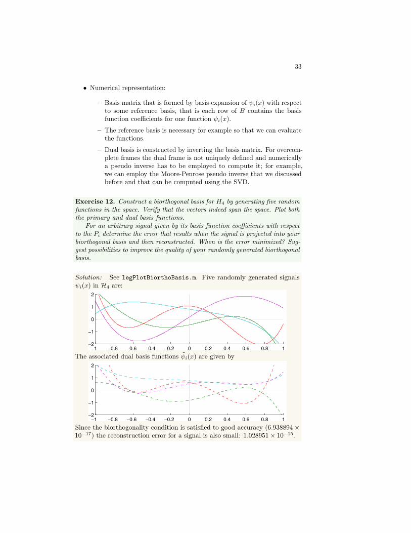
Exercise 12. Construct a biorthogonal basis for H4 by generating five randomfunctions in the space. Verify that the vectors indeed span the space. Plot boththe primary and dual basis functions.
For an arbitrary signal given by its basis function coefficients with respectto the Pi determine the error that results when the signal is projected into yourbiorthogonal basis and then reconstructed. When is the error minimized? Sug-gest possibilities to improve the quality of your randomly generated biorthogonalbasis.
Solution: See legPlotBiorthoBasis.m. Five randomly generated signalsψi(x) in H4 are:
−1 −0.8 −0.6 −0.4 −0.2 0 0.2 0.4 0.6 0.8 1−2
−1
0
1
2
The associated dual basis functions ψi(x) are given by
−1 −0.8 −0.6 −0.4 −0.2 0 0.2 0.4 0.6 0.8 1−2
−1
0
1
2
Since the biorthogonality condition is satisfied to good accuracy (6.938894×10⁻¹⁷) the reconstruction error for a signal is also small: 1.028951× 10⁻¹⁵.
34
Homework 5. In Example 1 we introduced the Mercedes Benz frame and inExercise 1 we generalized it to R3. When we employ the Cartesian coordinatesof the vectors as basis function coefficients for H2 with respect to the Legendrepolynomials Pi then this yields a frame the function space. Is this frame againa tight frame? Plot the signal f(x) corresponding to the expansions coefficientsf1 = 0.13, f2 = −0.56, f3 = 0.87.
Solution: This is again a tight frame since the Legendre polynomials providean isomorphism from H2 to R3.
TODO: Plot signal.
2.3 Approximation of Functions
In the foregoing we assumed that the function f(x) we would like to representin a basis or a frame lies in the space F(X) spanned by the representation,that is g(x) ∈ F(X). In practice, however, one often has a signal in some spaceF(X) and wants or needs to represent it in a“smaller” space F(X). For example,F(X) might be an infinite dimensional space and F(X) a finite dimensionalapproximation space spanned by a given basis.
• Distinguish linear vs. nonlinear.
– Linear: fixed approximation space.– Nonlinear: approximation space is determined based on the sig-
nal. Under certain conditions this is can be achieved surprisinglyeffectively.
The distinction between linear and nonlinear approximation is equivalent to astratification along other directions:
Linear Approximation Nonlinear Approximation
classical approximation theory modern approximation theory
Fourier / polynomial bases wavelet bases
optimal for smooth functionswith global regularity
optimal for functions with locallyvarying regularity and a finitenumber of discontinuities.
In the best case, one obtains even in the case of locally varying regularity andwith singularities the same order or approximation as in the globally smoothcase. The key to this result is an adaptation to the local properties of a functionso that the approximation only becomes “finer” where it is necessary. As we willsee in Chapter 2.3.3 only in 1D, and to a good extent in 2D, does this hold andin higher dimensions the question of how to effectively adapt to singularities isstill not resolved.
35
2.3.1 Linear Approximation
• Typically use of Fourier basis and polynomials to approximate functions.
• Optimal for sufficiently smooth function whose smoothness is constant isessentially constant over the domain.
• Approximation by retaining the first k coefficients (if necessary we canreorder basis functions). Error is given by remainder term.
For example for function in the Sovolev spaces H2([0, 1]), cf. Example 19,we have the following result.5
Theorem 2.1. Let f ∈ Hs([0, 1]) Then the linear N -term approximation error
εl(N, f) = ‖f − fN‖2
attained by approximating f in the Fourier basis over [0, 1] is εl(N, f) = o(N−2s)and this rate is asymptotically optimal.
The Fourier basis over [0, 1] used in the above theorem is discussed in Sec. 2.5.There we also show how to define Sobolev spaces for non-integer s. Theorem 2.1shows that the approximation rate increases as functions get smoother and thatwe have at least a quadratic convergence as long as our function is differentiable.However, the convergence rate becomes only linear when f has singularities.The same approximation rate of εl(N, f) = o(N−2s) can also be attained usingwavelets when these have q > s vanishing moments, see the next section for anintroduction to wavelets. Results analogous to Theorem 2.1 can be shown forother global regularity classes.
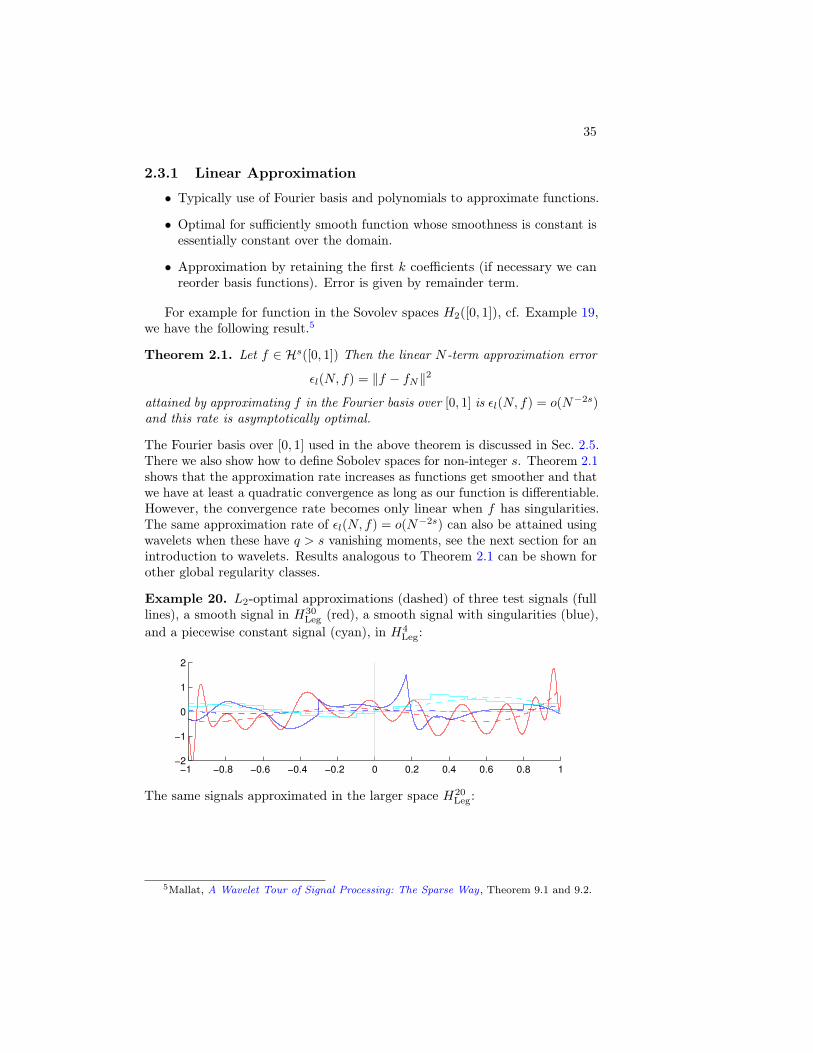
Example 20. L2-optimal approximations (dashed) of three test signals (fulllines), a smooth signal in H30
Leg (red), a smooth signal with singularities (blue),and a piecewise constant signal (cyan), in H4
Leg:
−1 −0.8 −0.6 −0.4 −0.2 0 0.2 0.4 0.6 0.8 1−2
−1
0
1
2
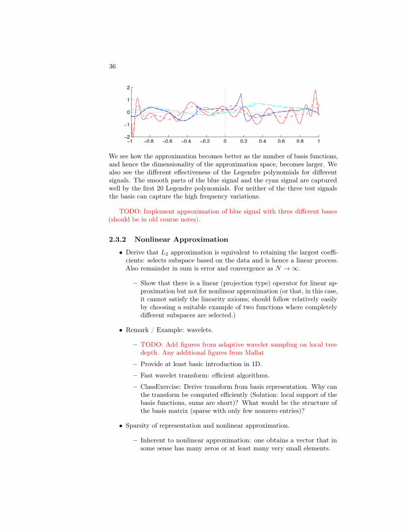
The same signals approximated in the larger space H20Leg:
5Mallat, A Wavelet Tour of Signal Processing: The Sparse Way, Theorem 9.1 and 9.2.
36
−1 −0.8 −0.6 −0.4 −0.2 0 0.2 0.4 0.6 0.8 1−2
−1
0
1
2
We see how the approximation becomes better as the number of basis functions,and hence the dimensionality of the approximation space, becomes larger. Wealso see the different effectiveness of the Legendre polynomials for differentsignals. The smooth parts of the blue signal and the cyan signal are capturedwell by the first 20 Legendre polynomials. For neither of the three test signalsthe basis can capture the high frequency variations.
TODO: Implement approximation of blue signal with three different bases(should be in old course notes).
2.3.2 Nonlinear Approximation
• Derive that L2 approximation is equivalent to retaining the largest coeffi-cients: selects subspace based on the data and is hence a linear process.Also remainder in sum is error and convergence as N →∞.
– Show that there is a linear (projection type) operator for linear ap-proximation but not for nonlinear approximation (or that, in this case,it cannot satisfy the linearity axioms; should follow relatively easilyby choosing a suitable example of two functions where completelydifferent subspaces are selected.)
• Remark / Example: wavelets.
– TODO: Add figures from adaptive wavelet sampling on local treedepth. Any additional figures from Mallat
– Provide at least basic introduction in 1D.
– Fast wavelet transform: efficient algorithms.
– ClassExercise: Derive transform from basis representation. Why canthe transform be computed efficiently (Solution: local support of thebasis functions, sums are short)? What would be the structure ofthe basis matrix (sparse with only few nonzero entries)?
• Sparsity of representation and nonlinear approximation.
– Inherent to nonlinear approximation: one obtains a vector that insome sense has many zeros or at least many very small elements.

37
– Moreover, this sparsity reflects the essential signal properties, forexample when wavelets are used it shows the spatial location ofsingularities.
– Essential difference to linear approximation: in some sense blind tothe signal (well, the basis function coefficients are not . . . but N-termapproximation).
• Language: more words allow to express ideas more succinctly. Similar,one wants to have highly sparse representations it is often useful to startwith an overcomplete frame and employ only those basis functions thatare useful to model the features of the signal.
– Another motivation for using frames.
– The prize that has to be paid is that there are no longer easy andefficient techniques to find the optimal set of basis functions thatshould be employed and one has to solve an optimization problem.
– Common numerical techniques are basis pursuit and matching pur-suit.6
To quantitatively analyze the effectiveness of approximations of nonlinearapproximation one needs a mathematical model of functions with local regularity,that is the type of functions where we have seen that nonlinear approximationcan be useful. One such model is Lipschitz regularity that can be seen as ageneralization of the Taylor series to functions that do not have a classicalderivative.
Definition 2.5. A function f : R→ R is pointwise Lipschitz α ≥ 0 at x ifthere exists a K > 0 and a polynomial px(x) of degree m = bαc such that7
|f(x)− px(x)| ≤ K|x− x|α , ∀x ∈ R. (2.14)
A function is f : R → R is uniformly Lipschitz α over [a, b] if the aboveLipschitz condition is satisfied for all x ∈ [a, b] for a K independent of x. TheLipschitz regularity of f is the supremum of the α such that f is Lipschitzα. The homogeneous Hölder α norm ‖f‖Cα of f is the infimum of the Kthat satisfy the Lipschitz condition in Eq. 2.14 for fixed α.
The exponent α in the above definition is also known as Hölder exponent.The definition is motivated by the Taylor series for an m times differentiablefunction where one has
|f(x)− px(x)| ≤ |x− x|m(
1
m!sup
u∈[x−x,x+x]
fm(u)
)(2.15)
6See (Mallat, A Wavelet Tour of Signal Processing: The Sparse Way, Chapter 12) fordetails.
7bαc is the largest integer smaller than α.
38
for all x ∈ [x− x, x+ x] where px(x) is the Taylor polynomial of order m,
px(x) =
m−1∑k=0
f (k)(x)
k!(x− x)k. (2.16)
When f ism times continuous differentiable then px(x) is the Taylor expansion off at x. If 0 ≤ α < 1 then px(x) = f(x), the “zero-th order Taylor approximation”,and the Lipschitz condition becomes
|f(x)− f(x)| ≤ K|x− x|α. (2.17)
Any 0 ≤ α < 1 characterizes the singularity type at x and α = 0 corresponds toa bounded but discontinuous function at x. Using this notion of local regularitywe can present a nonlinear analogue of Theorem 2.1:8
Theorem 2.2. Let f : [0, 1]→ R with K discontinuities and uniform Lipschitzα between the discontinuities with 1/2 < α < q then the linear approximationerror for wavelet with q vanishing moments is
εl(N, f) = O(K‖f‖2CαM−1
)and the error using nonlinear wavelet approximation is
εn(N, f) = O(‖f‖2CαM−2α
).
The discontinuities in the above definition are isolated points where α = 0 and‖ · ‖Cα is the homogeneous Hölder norm defined in Def. 2.5. Theorem 2.2 showsthat the convergence rate of nonlinear approximation is unaffected by the Ksingularities and one obtains still the same rate as if these were not present.This robustness to singularities is the most important practical advantage ofnonlinear approximation.
TODO: Example of nonlinear approximation of local spline signal withsingularities, analogous to Mallat (cf. Fig. 9.1 / 9.2).
The problem in practice is to find a “good” model class for a given application.
Remark 9 (Compressed Sensing). In the foregoing we only considered optimalapproximations in the L2 norm. However, an alternative to the L2 norm thathas become very popular recently is the L1 norm, mainly for applications incompressed sensing.9 The idea of the method is recover a signal that requiresm coefficients fi in a sparse representation from little more than m “samples”of the form 〈f, γi〉 where the γi are suitably chosen vectors such that 〈γi, ψi〉is nonzero for all ψi that are needed to represent f , at least with very highprobability. The condition 〈γi, ψi〉 6= 0 is known as incoherence condition in the
8Mallat, A Wavelet Tour of Signal Processing: The Sparse Way, Theorem 9.12.9(Candès, Romberg, and Tao, “Robust Uncertainty Principles: Exact Signal Reconstruction
from Highly Incomplete Frequency Information”; Donoho, “Compressed Sensing”), see forexample (Candès and Wakin, “An Introduction to Compressive Sampling”) for an introduction.
39
compressed sensing literature. Minimizing the L1 norm simultaneously findsthe coefficients that are nonzero and their numerical value. The price to be paidis that one requires an expensive optimization procedure which so far typicallyoutweighs any benefits. The remarkable aspect of compressed sensing is thatthe optimization is guaranteed to succeed with very high probability. Anotherapplication based on the same philosophy of minimizing the L1 norm is matrixcompletion from partial observations.10
2.3.3 From One to Higher Dimensions
Unfortunately, the approximation of signals becomes much more complex as thedimension increases. Part of the phenomenon is known as curse of dimension-ality . Additionally the structure of singularities becomes much more involvedas the dimension increases.
Remark 10. Dimension of bases space vs. dimension of function space.
Curse of Dimensionality 11
• Integral: with a tensor product one needs Nk quadrature points in kdimension: exponential dependence on dimension k
• Similar for approximation:
C0n−s/k ≤ δk(B(Hs))Lp(Ω) ≤ C1n
−s/k (2.18)
where B(Hs) is the unit ball in the Hilbert-Sobolev spaceHs and δn(B(Hs)),known as Kolmogorov width, corresponds to the nonlinear approximationerror εn(N, f) we considered before. We see that effective approximationsare only possible when s ≈ k, that is when the smoothness of the functionsincreases proportional to the dimensionality. This typically unrealistic andwe then have again an exponential dependence on the dimensionality.12
• For Rn or [0, 1]n and functions with classical regularity, sparse and multi-grid techniques provide a solution for moderate dimensionality up to aboutfive.13
– Finer notion of smoothness that allows for adaptivity.
• Very active area of research currently.
For more details see the survey by Donoho.14
10Candès and Recht, “Exact Matrix Completion via Convex Optimization”.11The term was coined by Bellmann (Adaptive Control Processes: A Guided Tour).12See (R. DeVore, Capturing Functions in High Dimensions) for details.13Bungartz and Griebel, “Sparse Grids”.14Donoho, “High-Dimensional Data Analysis: The Curses and Blessings of Dimensionality”.
40
Singularities in Higher Dimensions
• In 2D studied extensively for natural images.
– Singularities in 1D have one degree of freedom. In 2D singularitiescan be arbitrary curves. In higher dimensions this phenomenoncontinues. In nD one can have subsets of dimensions 1 · · · 1n.
– ClassExercise: Singularities for functions f : R → R3. What newtypes of singularities arise and find an example where these play arole? (Solution: 2D sub-manifolds in R3, appears for example inelasticity when cracks occur.
• Curvelets, bandlets, and shearlets provide representations that are theo-retically optimal, at least asymptotically, but not entirely practical.
– Also one requires frames to be able to effectively adapt to singulari-ties.
• High dimensional functions, 3D and beyond, with singularities largelyopen research problem.
2.4 Reproducing Kernels
In the last sections we ignored an important question: numerically central arethe basis function coefficients, which provide the coordinates of a signal in Rnthat can be used for numerical computations. However, the coefficients aregiven by
fi = 〈f(x), ψi(x)〉 =
∫X
f(x) ψi(x) dx. (2.19)
However, the integral is a continuous operation that cannot easily be evaluatedon a computer. The only information that can typically easily be obtainedin “computer problems” are function values f(x) for arbitrary points x and in“real world problems” measurements of the form mγ = 〈f, γ〉 for a measurementfunctional γ.15 For example, the measurement of a pixel sensor on a CCD chipcan be described by
m =
∫Pij
∫H2x
`(x, ω) pij(x, ω) dω dx (2.20)
where Pij is the area of the pixel, H2x the hemisphere above a point x on the
pixel, pij(x, ω) is the pixel response function for x and direction ω, and `(x, ω)the incoming light intensity. By defining an appropriate L2-inner product wecan write the above measurement also as
m = 〈`, pij〉 (2.21)
15This availability of functionals 〈f, γi〉 in many “real world” applications is one of thereasons for the relevance of compressed sensing, cf. Remark 9.

41
When such measurements are available we can construct the basis matrixto obtain the signal representation in a suitable basis or employ compressedsensing when the signal is sparse and we are willing to perform an expensiveoptimization, cf. Remark 9.
Unfortunately, in computer graphics one has typically synthetic problemswhere only pointwise information f(x) of the function of interest is available.In this section, we will discuss how to effectively work with signals when onlyfunction values f(xi) are available.
2.4.1 Point Evaluation Functionals
In Sec. 1.3 we discussed linear functionals on linear spaces V , that is mapsϕ : V → R that yield real number α(v) for elements v ∈ V and that are linear intheir arguments so that φ(av+ bw) = aϕ(v) + b φ(w) for v, w ∈ V and a, b ∈ R.The space of all such functionals was the dual space of V , and we distinguishedbetween the algebraic dual space V ∗ and the continuous dual space V . Alsorecall that for Hilbert spaces H, the Riesz representation theorem enables toidentify the continuous dual space H with H such that
ϕ(v) = 〈wϕ, v〉 (2.22)
where wϕ ∈ H is a unique element in H, cf. Theorem 1.1. We used this forexample in the construction of biorthogonal bases where the dual basis functionwas the realization of the coordinate functionals in H. An important functionalon function spaces, and the one of central importance for the present section isthe following.
Definition 2.6. Let F(X) be a function space defined over a set X. The pointevaluation functional Υx on F(X) at x ∈ X is for all f ∈ F(X)
Υx[f ] = f(x).
Example 21. Let C∞0 (R) be the set of compactly supported test functions onthe real line. The point evaluation functional on C∞0 (R) is the Dirac delta δxso that
Υx[f ] = δx[f ] = f(x)
for all f ∈ C∞0 (R). The Dirac delta δx is the prototype for a generalized functionor distribution in the sense of Schwartz . Such objects are useful for example todefine weak derivatives for functions that do not have derivatives in the classicalsense, such as a step function. The derivatives used in the definition of Sobolevspaces are typically such weak derivatives.
The above result can be extended to L2 since the space of test functionsC∞0 (R) is dense in Lp for 1 ≤ p <∞. This yields a definition of the Dirac deltaalso for L2(R) as it is commonly used in the engineering literature.
The above example shows that the point evaluation functional Υx is in generalnot continuous. However, in many applications and for computations the spaceswhere Υx is continuous are of particular.
42
Definition 2.7. Let H(X) be a Hilbert space where the point evaluation func-tional Υx is continuous. Then the reproducing kernel kbarx(x) at x is theunique function kx(x) ∈ H(X) such that
Υbarx[f ] = 〈f(x), kx(x)〉 , ∀f ∈ H(X) (2.23)
and H(X) is a reproducing kernel Hilbert space.
The remainder of the section will largely be concerned with studying thereproducing kernel Hilbert spaces introduced in the last section. Let us beginwith some examples that show that reproducing kernel Hilbert spaces are indeedpractically relevant.
Example 22. The Sobolev spaces H2(Rn) with s > n+ 1/2 are reproducingkernel Hilbert spaces.
Example 23. The Paley-Wiener space ΩB(R) of B-Fourier bandlimited func-tions for which the Fourier transform is supported only on [−B,B]. Thereproducing kernel is
sincB(x− x) =sin(B (x− x))
B x. (2.24)
Example 24. Every finite dimensional Hilbert space is a reproducing kernelHilbert space. The reproducing kernel is given below in Eq. 2.26
The last example is crucial for us since it shows that all function spaces relevantfor numerical computations are reproducing kernel Hilbert spaces. Before wecontinue, let us however consider an alternative perspective on the reproducingkernel. Let φini=1 be an orthonormal basis for H(X) and f ∈ H(X) be anarbitrary function. Then
f(x) =
n∑i=1
fi φi(x) (2.25a)
=
n∑i=1
〈f(x), φi(x)〉φi(x). (2.25b)
Using linearity of the inner product and that f(x) is independent of the sum-mation we obtain
f(x) =
n∑i=1
〈f(x), φi(x)φi(x)〉 (2.25c)
=
⟨f(x) ,
n∑i=1
φi(x)φi(x)
⟩. (2.25d)
Comparing Eq. 2.25d to Eq. 2.23 we see that we have to have
kx(x) = k(x, x) =
n∑i=1
φi(x)φi(x). (2.26)
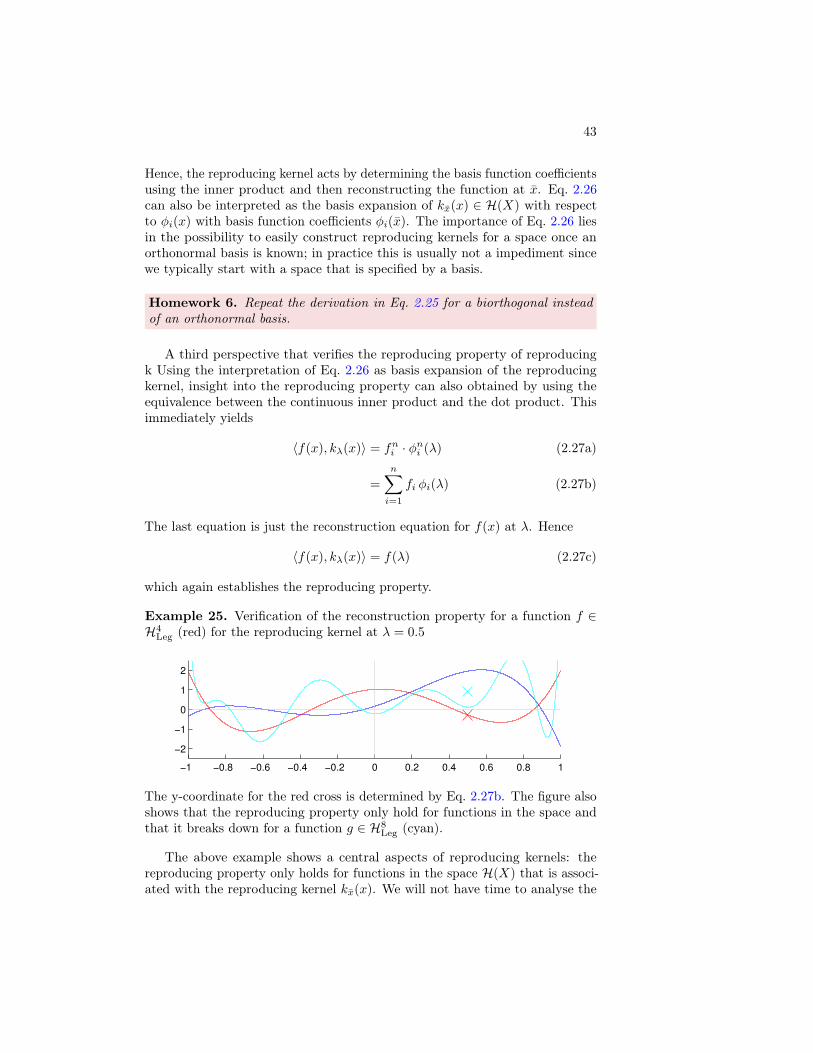
43
Hence, the reproducing kernel acts by determining the basis function coefficientsusing the inner product and then reconstructing the function at x. Eq. 2.26can also be interpreted as the basis expansion of kx(x) ∈ H(X) with respectto φi(x) with basis function coefficients φi(x). The importance of Eq. 2.26 liesin the possibility to easily construct reproducing kernels for a space once anorthonormal basis is known; in practice this is usually not a impediment sincewe typically start with a space that is specified by a basis.
Homework 6. Repeat the derivation in Eq. 2.25 for a biorthogonal insteadof an orthonormal basis.
A third perspective that verifies the reproducing property of reproducingk Using the interpretation of Eq. 2.26 as basis expansion of the reproducingkernel, insight into the reproducing property can also obtained by using theequivalence between the continuous inner product and the dot product. Thisimmediately yields
〈f(x), kλ(x)〉 = fni · φni (λ) (2.27a)
=
n∑i=1
fi φi(λ) (2.27b)
The last equation is just the reconstruction equation for f(x) at λ. Hence
〈f(x), kλ(x)〉 = f(λ) (2.27c)
which again establishes the reproducing property.
Example 25. Verification of the reconstruction property for a function f ∈H4
Leg (red) for the reproducing kernel at λ = 0.5
−1 −0.8 −0.6 −0.4 −0.2 0 0.2 0.4 0.6 0.8 1
−2
−1
0
1
2
The y-coordinate for the red cross is determined by Eq. 2.27b. The figure alsoshows that the reproducing property only hold for functions in the space andthat it breaks down for a function g ∈ H8
Leg (cyan).
The above example shows a central aspects of reproducing kernels: thereproducing property only holds for functions in the space H(X) that is associ-ated with the reproducing kernel kx(x). We will not have time to analyse the
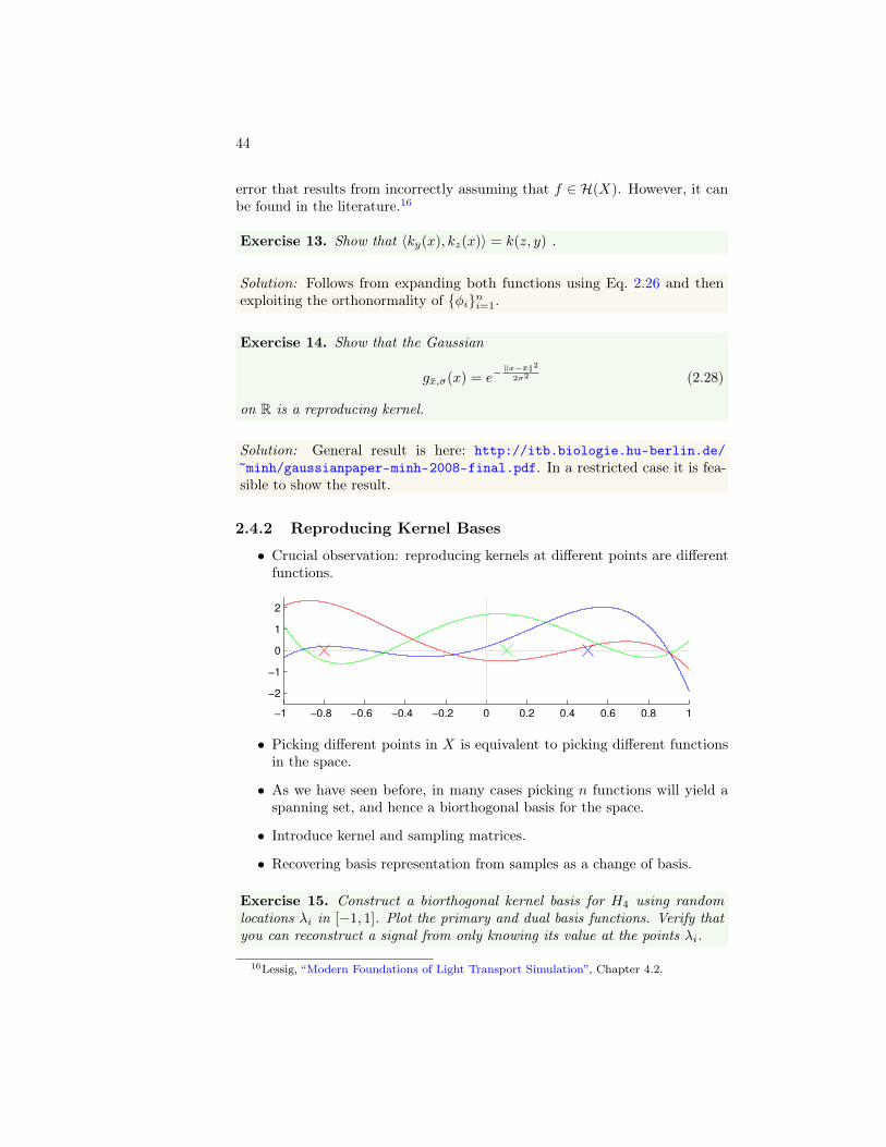
44
error that results from incorrectly assuming that f ∈ H(X). However, it canbe found in the literature.16
Exercise 13. Show that 〈ky(x), kz(x)〉 = k(z, y) .
Solution: Follows from expanding both functions using Eq. 2.26 and thenexploiting the orthonormality of φini=1.
Exercise 14. Show that the Gaussian
gx,σ(x) = e−‖x−x‖2
2σ2 (2.28)
on R is a reproducing kernel.
Solution: General result is here: http://itb.biologie.hu-berlin.de/~minh/gaussianpaper-minh-2008-final.pdf. In a restricted case it is fea-sible to show the result.
2.4.2 Reproducing Kernel Bases
• Crucial observation: reproducing kernels at different points are differentfunctions.
−1 −0.8 −0.6 −0.4 −0.2 0 0.2 0.4 0.6 0.8 1
−2
−1
0
1
2
• Picking different points in X is equivalent to picking different functionsin the space.
• As we have seen before, in many cases picking n functions will yield aspanning set, and hence a biorthogonal basis for the space.
• Introduce kernel and sampling matrices.
• Recovering basis representation from samples as a change of basis.
Exercise 15. Construct a biorthogonal kernel basis for H4 using randomlocations λi in [−1, 1]. Plot the primary and dual basis functions. Verify thatyou can reconstruct a signal from only knowing its value at the points λi.
16Lessig, “Modern Foundations of Light Transport Simulation”, Chapter 4.2.
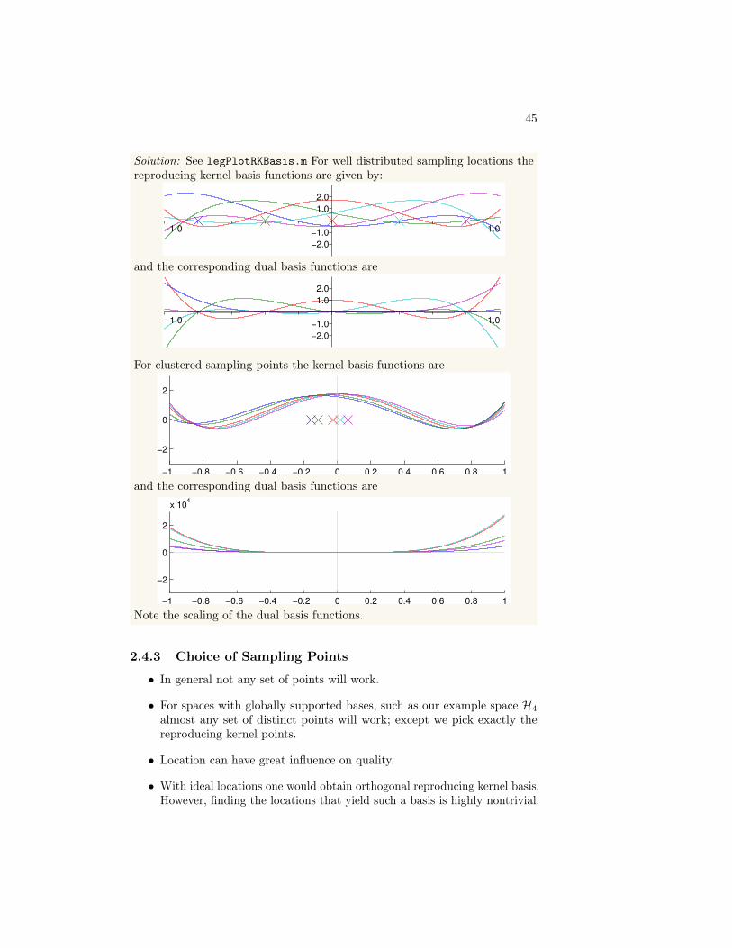
45
Solution: See legPlotRKBasis.m For well distributed sampling locations thereproducing kernel basis functions are given by:
−1.0 1.0
−2.0
−1.0
1.0
2.0
and the corresponding dual basis functions are
−1.0 1.0
−2.0
−1.0
1.0
2.0
For clustered sampling points the kernel basis functions are
−1 −0.8 −0.6 −0.4 −0.2 0 0.2 0.4 0.6 0.8 1
−2
0
2
and the corresponding dual basis functions are
−1 −0.8 −0.6 −0.4 −0.2 0 0.2 0.4 0.6 0.8 1
−2
0
2
x 104
Note the scaling of the dual basis functions.
2.4.3 Choice of Sampling Points
• In general not any set of points will work.
• For spaces with globally supported bases, such as our example space H4
almost any set of distinct points will work; except we pick exactly thereproducing kernel points.
• Location can have great influence on quality.
• With ideal locations one would obtain orthogonal reproducing kernel basis.However, finding the locations that yield such a basis is highly nontrivial.
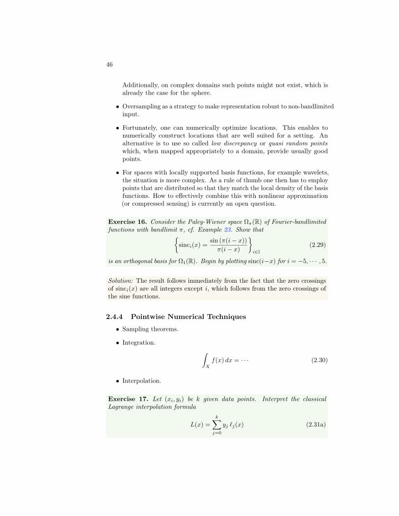
46
Additionally, on complex domains such points might not exist, which isalready the case for the sphere.
• Oversampling as a strategy to make representation robust to non-bandlimitedinput.
• Fortunately, one can numerically optimize locations. This enables tonumerically construct locations that are well suited for a setting. Analternative is to use so called low discrepancy or quasi random pointswhich, when mapped appropriately to a domain, provide usually goodpoints.
• For spaces with locally supported basis functions, for example wavelets,the situation is more complex. As a rule of thumb one then has to employpoints that are distributed so that they match the local density of the basisfunctions. How to effectively combine this with nonlinear approximation(or compressed sensing) is currently an open question.
Exercise 16. Consider the Paley-Wiener space Ωπ(R) of Fourier-bandlimitedfunctions with bandlimit π, cf. Example 23. Show that
sinci(x) =sin (π(i− x))
π(i− x)
i∈I
(2.29)
is an orthogonal basis for Ω1(R). Begin by plotting sinc(i−x) for i = −5, · · · , 5.
Solution: The result follows immediately from the fact that the zero crossingsof sinci(x) are all integers except i, which follows from the zero crossings ofthe sine functions.
2.4.4 Pointwise Numerical Techniques
• Sampling theorems.
• Integration. ∫X
f(x) dx = · · · (2.30)
• Interpolation.
Exercise 17. Let (xi, yi) be k given data points. Interpret the classicalLagrange interpolation formula
L(x) =
k∑j=0
yj `j(x) (2.31a)
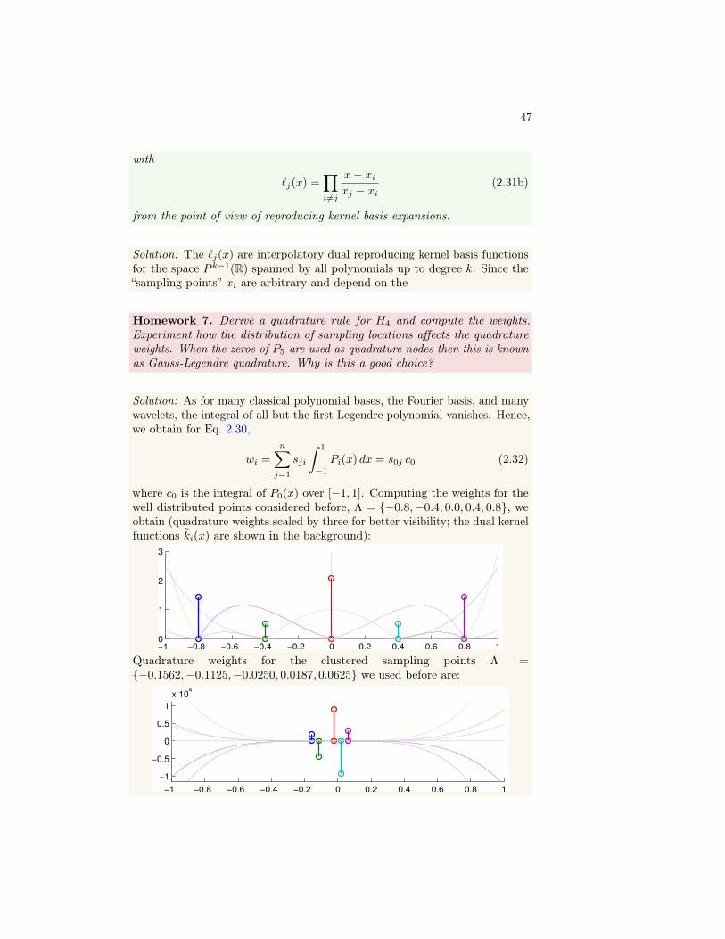
47
with
`j(x) =∏i 6=j
x− xixj − xi
(2.31b)
from the point of view of reproducing kernel basis expansions.
Solution: The `j(x) are interpolatory dual reproducing kernel basis functionsfor the space P k−1(R) spanned by all polynomials up to degree k. Since the“sampling points” xi are arbitrary and depend on the
Homework 7. Derive a quadrature rule for H4 and compute the weights.Experiment how the distribution of sampling locations affects the quadratureweights. When the zeros of P5 are used as quadrature nodes then this is knownas Gauss-Legendre quadrature. Why is this a good choice?
Solution: As for many classical polynomial bases, the Fourier basis, and manywavelets, the integral of all but the first Legendre polynomial vanishes. Hence,we obtain for Eq. 2.30,
wi =
n∑j=1
sji
∫ 1
−1
Pi(x) dx = s0j c0 (2.32)
where c0 is the integral of P0(x) over [−1, 1]. Computing the weights for thewell distributed points considered before, Λ = −0.8,−0.4, 0.0, 0.4, 0.8, weobtain (quadrature weights scaled by three for better visibility; the dual kernelfunctions ki(x) are shown in the background):
−1 −0.8 −0.6 −0.4 −0.2 0 0.2 0.4 0.6 0.8 10
1
2
3
Quadrature weights for the clustered sampling points Λ =−0.1562,−0.1125,−0.0250, 0.0187, 0.0625 we used before are:
−1 −0.8 −0.6 −0.4 −0.2 0 0.2 0.4 0.6 0.8 1
−1
−0.5
0
0.5
1
x 104
48
Note that the scaling of the weights differs by four order of magnitude. Addi-tionally, for clustered sampling points one has positive and negative weightswhich is numerically undesirable.17 As an example, we can integrate the Leg-endre polynomials Pi(x), 1 ≤ x ≤ 4, where we know that the integral vanishes.With the well distributed sampling points we obtain in double precision anaverage error of −6.94× 10⁻¹⁸ while the clustered points yield −1.14× 10⁻¹³.The four digits that are lost compared to machine precision for the clusteredpoints are roughly described by the magnitude of the quadrature weights.
The quadrature nodes that are classically used for integration in the spacesHnLeg are the n zero crossings of the Legendre polynomial Pn+1 of degree n+ 1.The quadrature rule is then known as Gauss-Legendre quadrature. Using thezero crossings of Pn+1 increases the accuracy of the quadrature rule, as canbe seen using an error analysis.18
Exercise 18. Devise an interpolation technique that employs the values f(λi)of a function and its derivatives f ′(λi).
TODO: Work out details
• Derivative is a linear operator so it commutes with the basis representa-tion.
• One can reconstruct a reproducing kernel for derivative information.
• Combining these ideas should yield the result.
Example 26. In this example we will show how reproducing kernels enablea functional analytic interpretation of Monte Carlo integration. For this, wewill also require the concept of a characteristic basis and its connection toreproducing kernels.
Let X be a set. The characteristic function χY :X → R for a subset Y ⊂ Xis defined as
χY (x) =
1 if x ∈ Y0 otherwise . (2.33)
A partition of X is the collection of disjoint subsets Xi, i = 1 · · ·n, of X suchthat their union forms again X, that is
X =
n⋃i=1
Xi. (2.34)
When we denote the characteristic function for each element Xi of a partition byχi(x) then we obtain a basis for the space span(χi(x)) = Hχ ≡ Hχ(X) ⊂ L2(X).Since Hχ(X) is a closed subspace of L2(X) it is a Hilbert space equipped withthe L2 inner product. We call χi(x)ni=1 a characteristic basis.
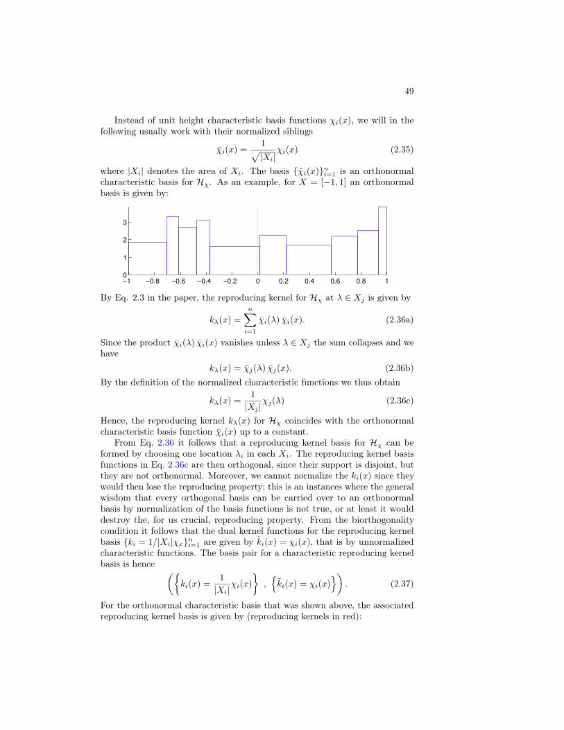
49
Instead of unit height characteristic basis functions χi(x), we will in thefollowing usually work with their normalized siblings
χi(x) =1√|Xi|
χi(x) (2.35)
where |Xi| denotes the area of Xi. The basis χi(x)ni=1 is an orthonormalcharacteristic basis for Hχ. As an example, for X = [−1, 1] an orthonormalbasis is given by:
−1 −0.8 −0.6 −0.4 −0.2 0 0.2 0.4 0.6 0.8 10
1
2
3
By Eq. 2.3 in the paper, the reproducing kernel for Hχ at λ ∈ Xj is given by
kλ(x) =
n∑i=1
χi(λ) χi(x). (2.36a)
Since the product χi(λ) χi(x) vanishes unless λ ∈ Xj the sum collapses and wehave
kλ(x) = χj(λ) χj(x). (2.36b)By the definition of the normalized characteristic functions we thus obtain
kλ(x) =1
|Xj |χj(λ) (2.36c)
Hence, the reproducing kernel kλ(x) for Hχ coincides with the orthonormalcharacteristic basis function χi(x) up to a constant.
From Eq. 2.36 it follows that a reproducing kernel basis for Hχ can beformed by choosing one location λi in each Xi. The reproducing kernel basisfunctions in Eq. 2.36c are then orthogonal, since their support is disjoint, butthey are not orthonormal. Moreover, we cannot normalize the ki(x) since theywould then lose the reproducing property; this is an instances where the generalwisdom that every orthogonal basis can be carried over to an orthonormalbasis by normalization of the basis functions is not true, or at least it woulddestroy the, for us crucial, reproducing property. From the biorthogonalitycondition it follows that the dual kernel functions for the reproducing kernelbasis ki = 1/|Xi|χxni=1 are given by ki(x) = χi(x), that is by unnormalizedcharacteristic functions. The basis pair for a characteristic reproducing kernelbasis is hence (
ki(x) =1
|Xi|χi(x)
,ki(x) = χi(x)
). (2.37)
For the orthonormal characteristic basis that was shown above, the associatedreproducing kernel basis is given by (reproducing kernels in red):
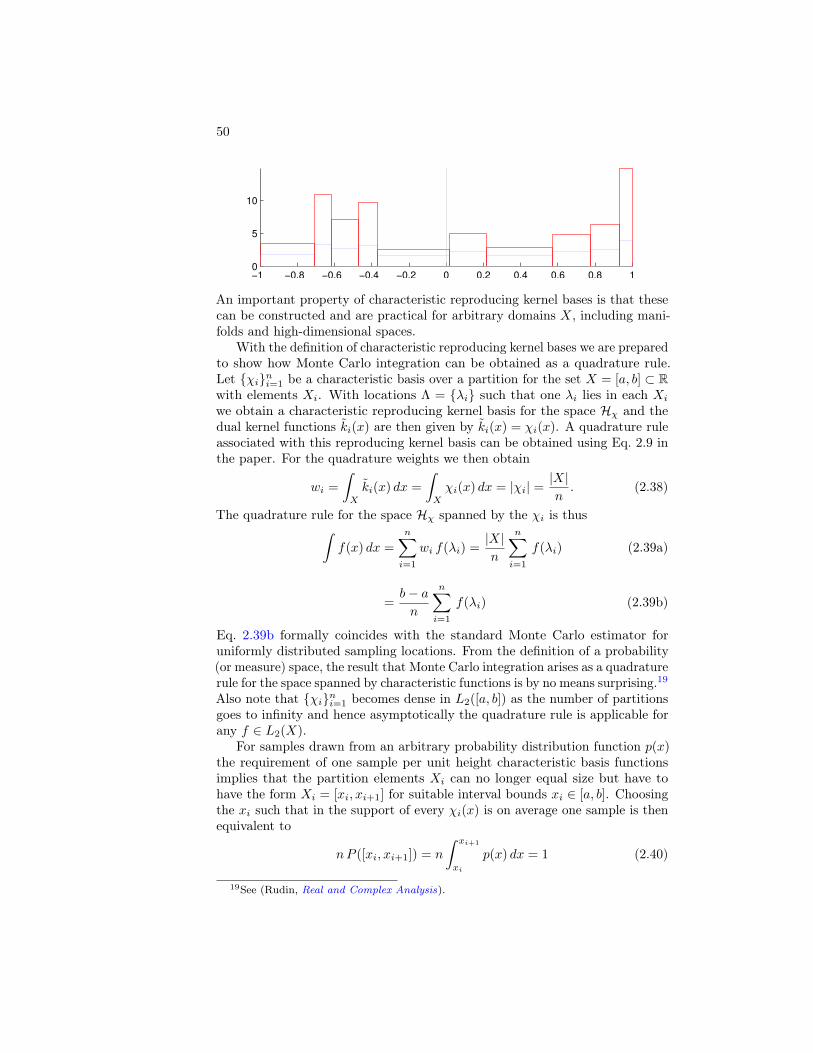
50
−1 −0.8 −0.6 −0.4 −0.2 0 0.2 0.4 0.6 0.8 10
5
10
An important property of characteristic reproducing kernel bases is that thesecan be constructed and are practical for arbitrary domains X, including mani-folds and high-dimensional spaces.
With the definition of characteristic reproducing kernel bases we are preparedto show how Monte Carlo integration can be obtained as a quadrature rule.Let χini=1 be a characteristic basis over a partition for the set X = [a, b] ⊂ Rwith elements Xi. With locations Λ = λi such that one λi lies in each Xi
we obtain a characteristic reproducing kernel basis for the space Hχ and thedual kernel functions ki(x) are then given by ki(x) = χi(x). A quadrature ruleassociated with this reproducing kernel basis can be obtained using Eq. 2.9 inthe paper. For the quadrature weights we then obtain
wi =
∫X
ki(x) dx =
∫X
χi(x) dx = |χi| =|X|n. (2.38)
The quadrature rule for the space Hχ spanned by the χi is thus∫f(x) dx =
n∑i=1
wi f(λi) =|X|n
n∑i=1
f(λi) (2.39a)
=b− an
n∑i=1
f(λi) (2.39b)
Eq. 2.39b formally coincides with the standard Monte Carlo estimator foruniformly distributed sampling locations. From the definition of a probability(or measure) space, the result that Monte Carlo integration arises as a quadraturerule for the space spanned by characteristic functions is by no means surprising.19Also note that χini=1 becomes dense in L2([a, b]) as the number of partitionsgoes to infinity and hence asymptotically the quadrature rule is applicable forany f ∈ L2(X).
For samples drawn from an arbitrary probability distribution function p(x)the requirement of one sample per unit height characteristic basis functionsimplies that the partition elements Xi can no longer equal size but have tohave the form Xi = [xi, xi+1] for suitable interval bounds xi ∈ [a, b]. Choosingthe xi such that in the support of every χi(x) is on average one sample is thenequivalent to
nP ([xi, xi+1]) = n
∫ xi+1
xi
p(x) dx = 1 (2.40)
19See (Rudin, Real and Complex Analysis).
51
which with y ∈ [xi, xi+1] is to zeroth order
n (p(y) (xi+1 − xi)) = 1. (2.41)
With λi being the samples in the support of χi one thus has |χi| = xi+1 − xi =1/(n p(λi)). The quadrature rule with samples distributed according to p(x) istherefore ∫
f(x) dx =1
n
n∑i=1
f(λi)
p(λi)(2.42)
Eq. 2.42 formally coincides with the standard Monte Carlo estimator for impor-tance sampling.
2.5 Linear Operators on Function Spaces
We have already abstractly considered linear maps in Chapter 1.5. In thissection we will specialize to the case of linear spaces that are function spaces.One then typically speaks about linear operators or just operators. Let us beginby considering some examples.
Example 27. Linear functional is a special case of a linear operator that wealready considered. Every linear functional ϕ ∈ H∗ can be realized as
ϕ[f ] =
∫X
kϕ(x) f(x) dx (2.43)
for a sufficiently general integral kernel kϕ(x), which might no longer be afunction in the classical sense. This is a generalization of the Riesz representationtheorem in Theorem 1.1.
We have already seen simple examples for nonlinear operators in Example 5.We will see nonlinear differential and integral operators in the following sections.
2.5.1 Differential Operators
• We will only briefly discuss differential operators here and have a moredetailed discussion in the next chapter.
– It will be a good warm-up for the things that come later.
• This is the theory of partial differential equations that describe theevolution (typically time evolution) of “fields”, that is continuous, notnecessarily scalar functions describing quantities of physical interest.
– All things in science are describe by ordinary or partial differentialequations; at least in the hard sciences, and in particular in physics.
– Obviously, our focus will be on linear partial differential equations.We will remark on nonlinear ones, which can be seen as a naturalgeneralization, in Remark 12.
52
• Before we continue and discuss in more detail the theoretical aspects, letus consider an example
Example 28. Autonomous transport equation for function ρ :M⊂ R3 → R,for example fluid mass density in fluid mechanics, for a divergence free velocityvector field ~v :M⊂ R3 → R320 is given by
∂ρ
∂t+ ~v · ∂ρ
∂x= 0. (2.44)
Interpretation:
• The mathematical formula is quite useless if one cannot interpret theequation and put some meaning into it.
• So called Eulerian representation.
• Right hand side is zero because it describes a conservation equation. Herethe mass density ρ is globally conserved, that is mass is neither creatednor destroyed.
• The equation is somewhat easier to interpret when it is written as
∂ρ
∂t= ~v · ∂ρ
∂x. (2.45)
• The change of ρ(x) at x in time, this is what the derivative on the lefthand side says, is given by the divergence on the right hand side. We willsee what the divergence means later but the general form in the Eulerianrepresentation, the change of the quantity in time is expressed by somedifferential operator is very important. To complete the picture one hasto understand the differential operator. In the above case this is best donelater when we introduced a differential operator known as Lie derivative.
• TODO: figure
General form of Linear Partial Differential Equations
• Derivative of functions on the real line is well known.
• We can look at it as a map
d
dx: F(R)→F(R) (2.46)
where F(R),F(R) are suitable function spaces.
• Hence, d/dx is an operator.
20See Chapter 3.4 for the definition of divergence and its meaning.
53
• Is d/dx also a linear operator or map? By the standard rules of differenti-ation, this is indeed the case:
d
dx
(a f(x) + b g(x)
)= a
df
dx+ b
dg
dx. (2.47)
• Remark: d/dx vs. ∂/∂x. We will typically use the latter in the following.
• We define Ck(R) as the class of k-times continuously differentiable func-tions. Then
d
dx: Ck+1(R)→ Ck(R) (2.48)
and d/dx : C∞ → C∞
• A general linear differential operator on Rn of order k acting on a functionf : Rn → R has the form
Ax =∑|α|≤k
cα(x)∂
∂xα(2.49)
where α = (α1, · · ·αn) is a multi-index that determines the degree of thederivative in each dimension. In 2D a differential operator of degree 1can for example have
α = (0, 0)∂
∂xαf =
∂
∂x01 x
02
f = f (2.50a)
α = (1, 0)∂
∂xαf =
∂
∂x11 x
02
f =∂f
∂x1(2.50b)
α = (0, 1)∂
∂xαf =
∂
∂x01 x
12
f =∂f
∂x2(2.50c)
α = (1, 1)∂
∂xαf =
∂
∂x01 x
12
f =∂f
∂x1 x2(2.50d)
The cα(x) are coefficient functions that can on the position x; in thesimplest case these are just constants.
• This is the coordinate form usually used in the theory of partial differentialequations.
• Remark (appropriate function spaces): We can still defined Ck but itsin general not a very useful notion. Most functions have a differentdifferentiability class in each dimension. Anisotropic function space thatallow for different differentiability, and more general regularity, at eachpoint and each coordinate direction one needs much more complicatedspaces. For questions like existence of well defined solutions one also needsSobolev spaces that provide additional control over the magnitude of thederivatives.
54
Example 29. Concrete example: Laplacian in Rn
∆f =
n∑i=1
∂2f
∂x2i
(2.51)
it is the sum of the pure or unmixed second partial derivatives; to be even moreconcrete, in R3 we have
∆f =
n∑i=1
∂f
∂x2i
=∂2f
∂x21
+∂2f
∂x22
+∂2f
∂x23
. (2.52)
Initial value problem and boundary conditions
• One knows the differential equation, the “law”, for example for the timeevolution, and one is interested how the system develops for finite times.
• The pde only gives evolution for infinitesimal times, and one has to extendthis to finite times.
• Alternatively, one might be interested in the steady state, see Remark 11.
Boundary conditions:
• On a compact domain, as one typically considers in applications, thedifferential equations require boundary to be well defined, that is a de-scription of what happens to the function at the boundary where thederivative is not well defined. For example, we could require that f(x)and all derivatives of f(x). Clearly the boundary conditions will affect thesolution, possibly over the whole domain. The most common boundaryconditions are:
– Dirichlet boundary conditions: the function value at the boundaryis specified.
– Neumann boundary conditions: The derivative of f(x) in the normaldirection is specified (physically, this corresponds to in and out fluxfrom a domain, which makes them physically very important).
– TODO: figure
• Periodic boundary conditions with period z: f(x + z) = f(x) whichin particular means that one identifies points on “opposite boundaries”TODO: figure; this corresponds to a torus.
Solving:
• Solving a differential equation for given initial data can rarely be doneanalytically.
55
• We will talk about Green’s functions as an analytic approach to thesolution and about Galerkin projection for the numerical solution later.Additionally, the method of characteristics is often very useful, cf. Exam-ple 45.
• As a rule of thumb, and we talk about this later in more detail, one shouldunderstand as much about the application and mathematical structure ofa partial differential equation before attempting to solve it numerically.
• There are recipes like finite element methods but they are far fromfoolproof.
• Mathematics: tries to prove existence of solutions. No general result.
– Millenium prize for Navier-Stokes. Terence Tao’s recent result forNavier-Stokes.
• Analytic techniques like separation of variables. Subject of a specializedcourse on the subject.
– If possible, often a useful step before numerical treatment.
Remark 11. We see how the above partial differential equations describe timeevolution. A stationary or steady state solution is also often of interest. Itmeans that the quantity of interest, say φ(x, t) does not change. Hence, onehas to have
∂φ
∂t= 0. (2.53)
For example, for the fluid density in Eq. 2.44 the steady state is given by
∂ρ
∂t= 0 = ~v · ∂ρ
∂x. (2.54)
Note that this by no means implies that the fluid velocity vanishes or that nomass is transported by the fluid. What is steady or time invariant is the valueof the density at the location x.
We will leave it at this for the moment and return to the subject later.However, before we do this let us look at some examples:
Example 30. The heat equations for a function u :M⊂ R3 → R, for examplethe temperature at x ∈M, is given by
∂u
∂t+ ∆u = 0 (2.55)
As the name suggests, it describes the diffusion of heat in an environment. Asboundary conditions we can for example use Neumann boundary conditionswith
∂u(x)
∂~n(x)
∣∣∣∣∂M
= 0 (2.56)

56
which corresponds to a perfect insulator, that is no heat flows through theboundary.
TODO: Figure with time evo. From Wikipedia? 1D or 2D?
Example 31. Scalar wave equation for φ :M⊂ R3 → R
∂2φ
∂t2+ ∆φ = 0 (2.57)
The equation is for example central to acoustics.The scalar wave equation in Eq. 2.57 is second order and hence more difficult
to interpret than the autonomous transport equation in Example 28 where wecould find an interpretation. However, by introducing
~s =∂φ
∂t: M⊂ R3 → R (2.58a)
~r =∂φ
∂x: M⊂ R3 → R3 (2.58b)
as independent variables, Eq. 2.57 becomes
∂s
∂t=
3∑i=1
∂r
∂xi(2.59a)
∂r
∂t=∂s
∂x. (2.59b)
Hence, we have two first order transport equation that can be interpretedsimilarly to the autonomous transport equation in Example 28. The additionalcomplexity of the second order equation is thereby “hidden” in the couplingbetween the two equations. 21
Exercise 19. Write the scalar wave equation in the form of a general lineardifferential operator in Eq. 2.49 by using space-time coordinates where x0 = t.
The wave equation can be seen as a space-time Laplace operator,
Wf =
n∑i=0
∂2f
∂x2i
. (2.60)
However, as we will see later the time coordinate does have a different behaviourthan the space coordinates so that the properties of W are quite different.
• We will return to the above examples in Chapter 3 where we will reconsiderthem from a more conceptual perspective.
21The reader might have seen something similar already in the context of ordinary dif-ferential equations where one can also reduce nth order equations to a system of first orderequations. The latter ones are typically used for numerical integration.
57
• Laplace operator arose as part of the heat equation and the Laplaceequation. It also plays an important role, and has found a many, manyapplications in computer graphics. We will also consider it again fromvarious perspective below.
Let us conclude this section with going beyond the linear regime and brieflydiscussing nonlinear differential operators.
Remark 12. As an extension of Eq. 2.49, the most important examples ofnonlinear differential operators are of the form
N(f) =
∑|α|<k
ci(f)∂
∂xα
f (2.61)
where the ai(f) depend on the argument f and α = (α1, · · · , αn) is againa multi-index. Such nonlinear operators have a multitude of applications inscience. For example, the Euler equation, which describes the time evolution ofthe velocity vector field ~v(x, t) of an ideal fluid, is given by
∂~v
∂t+∇~v ~v = ∇p (2.62)
where ~v is the fluid velocity vector field and p the pressure, and we see thatin the second term on the left hand side ~v is part of the differential operatorand the vector-valued function the operator acts on. We will return to theEuler equation again in later chapters. Nonlinear generalization of the lineardifferential and integral operators that we consider below in Chapter 2.5.1 andChapter 2.5.2.
2.5.2 Integral Operators
• The second class of linear operators we will consider are integral operators.We will see in the following when we consider Green’s functions that inmany instances an intimate connection between differential and integraloperators exists.
• Definition: given by K : F(X)→F (Y ):
g(y) = K(f) =
∫X
k(x, y) f(x) dx (2.63)
and k(x, y) is known as the kernel of the integral operator.
Example 32. Linear functionals are (somewhat degenerate) example whereF (Y ) = R
Example 33. Hilbert-Schmidt integral operators.
58
• The kernel is in L2 as a function of x and y. This ensures that theoperator is compact, and hence well behaved in a sense somewhat beyondour discussion.
• When the kernel is symmetric then the operator is self-adjoint.
• Compactness and self-adjointness are the essential condition for spectraltheorem to apply, cf. Theorem 1.3. Hence, Hilbert-Schmidt operatorshave a well defined eigen decomposition, and, moreover, the necessaryconditions are easy to verify.
Hilbert-Schmidt operators are the generalization of the above integral operatorsthat have the same convenient properties.
Exercise 20. Show that on L2(X) a Hilbert-Schmidt operator is self-adjointwhen the kernel is symmetric.
Solution: L2 inner product and integral of operator action can change. L2
integrability ensures that Fubini’s theorem can be used and the interchange isactually valid. TODO: Verify the idea
Example 34. TODO: Rendering: scattering as Hilbert-Schmidt operator.
Remark 13. By a celebrated result by Laurent Schwartz, every “reasonable”operator on the space of compactly supported C∞ test functions, cf. Ex. 21, canbe realized as an integral operator. This in particular also includes differentialoperators. As an example, the integral representation of the identity operator is
Id(f)|x =
∫X
δx(x) f(x) dx (2.64)
where δx(x) is the Dirac delta distribution, cf. again Ex. 21.
Example 35. Markov chain. Integral operator K : F(X)→ F(X) on a spacewith λ = 1 as largest eigenvalue, that is
f(y) =
∫X
k(x, y) f(x) dx. (2.65)
Integral kernel k(x, y) then models the transition probability between the statesx ∈ X and y ∈ X. Hence, it also satisfies
1 =
∫X
k(x, y)dy (2.66)
to ensure that the transition probability is indeed a probability. The eigenfunc-tion f(x) associated with λ = 1 is the steady state distribution. The terminologycomes from the fact that f(x) is invariant under the integral operator.
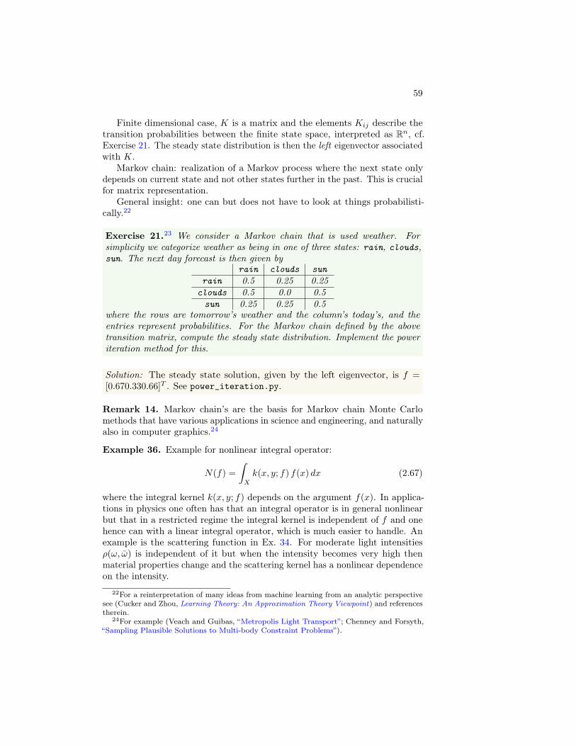
59
Finite dimensional case, K is a matrix and the elements Kij describe thetransition probabilities between the finite state space, interpreted as Rn, cf.Exercise 21. The steady state distribution is then the left eigenvector associatedwith K.
Markov chain: realization of a Markov process where the next state onlydepends on current state and not other states further in the past. This is crucialfor matrix representation.
General insight: one can but does not have to look at things probabilisti-cally.22
Exercise 21.23 We consider a Markov chain that is used weather. Forsimplicity we categorize weather as being in one of three states: rain, clouds,sun. The next day forecast is then given by
rain clouds sunrain 0.5 0.25 0.25
clouds 0.5 0.0 0.5sun 0.25 0.25 0.5
where the rows are tomorrow’s weather and the column’s today’s, and theentries represent probabilities. For the Markov chain defined by the abovetransition matrix, compute the steady state distribution. Implement the poweriteration method for this.
Solution: The steady state solution, given by the left eigenvector, is f =[0.670.330.66]T . See power_iteration.py.
Remark 14. Markov chain’s are the basis for Markov chain Monte Carlomethods that have various applications in science and engineering, and naturallyalso in computer graphics.24
Example 36. Example for nonlinear integral operator:
N(f) =
∫X
k(x, y; f) f(x) dx (2.67)
where the integral kernel k(x, y; f) depends on the argument f(x). In applica-tions in physics one often has that an integral operator is in general nonlinearbut that in a restricted regime the integral kernel is independent of f and onehence can with a linear integral operator, which is much easier to handle. Anexample is the scattering function in Ex. 34. For moderate light intensitiesρ(ω, ω) is independent of it but when the intensity becomes very high thenmaterial properties change and the scattering kernel has a nonlinear dependenceon the intensity.
22For a reinterpretation of many ideas from machine learning from an analytic perspectivesee (Cucker and Zhou, Learning Theory: An Approximation Theory Viewpoint) and referencestherein.
24For example (Veach and Guibas, “Metropolis Light Transport”; Chenney and Forsyth,“Sampling Plausible Solutions to Multi-body Constraint Problems”).
60
Green’s Functions Let us begin by recalling the spectral theory that weintroduced in Chapter 1.5.2. and that immediately applies to linear operators.
• Recall spectral theorem for operators.
• In our formulation is immediately applies to operators.
• Requires compactness. Generalizations exist but too technical for ourpurposes. For example, in general continuous spectrum possible, which ismuch more difficult to work with (although we will encounter it when wetalk about the Fourier transform). Also, there might be no eigenfunctionsat all, or they are or can only defined implicitly.
Definition 2.8. Green’s function
Proposition 2.1. Eigenvector expansion of Green’s function
Exercise 22. Show the above proposition.
Solution: TODO: Show it.
Example 37. Poisson equation
∆f = g (2.68)
The Laplace equation is g = 0, that is the homogenous form of the equation.On R3 the Green’s function of the Poisson equation is given by
G(x, x) = − 1
4π
1
|x− x|. (2.69)
The Poisson and Laplace equations arise in a multitude of applications in CG.
• TODO: Provide a concrete example. For example surface reconstruction.Where was Green’s function actually used?
Homework 8. Eigenfunction’s of heat operator H are Fourier and eigenvaluesare . . .Numerically construct the Green’s function. For this, experiment withthe number of eigenfunctions that are needed. Guess the analytic form
Solution: TODO: Implement!
How to solve differential equations using Green’s functions:
• Sometimes, like in the case of the heat equation, the Green’s function hasan analytic form and this form is sufficiently nice to enable an analyticsolution.
– Restricted to simple / symmetric domains.

61
– “Canonical” differential equations. Although the number of “useful”differential equations is surprisingly small and one encounters thesame equation typically over and over again.
• In principal one can use quadrature since one has an integral. However,this only yields the solution at single point. Galerkin projection, whichwill be discussed in the next section,
2.5.3 Galerkin Projection
Galerkin projection25
• Very general approach to obtain finite dimensional representations foroperator equations.
– Classical form and the once we will discuss are for linear operatorequations but also extensions for nonlinear ones.
Let A : F → G be a linear operator between separable Hilbert spaces F andG, that is
Af = g. (2.70)
Furthermore assume that ϕi∞i=1 is an orthonormal basis for F and ψj∞j=1 isan orthonormal basis for G. For Galerkin projection, we project Eq. 2.70 ontoψj ,
〈Af, ψj〉 = 〈g, ψj〉 (2.71a)
and expand f in ϕi∞i=1,⟨A(∑
i fi ϕi
), kj
⟩= 〈g, ψj〉 . (2.71b)
By linearity we then have
∞∑i=1
fi 〈Aϕi, ψj〉 = 〈g, ψj〉 . (2.71c)
and by defining Aij = 〈Aϕi, ψj〉 we obtain
∞∑i=1
fiAij = gj . (2.71d)
• The Aij form an infinite matrix.
25Galerkin, “On Electrical Circuits for the Approximate Solution of the Laplace Equation”;Petrov, “Application of the Method of Galerkin to a Problem Involving the Stationary Flowof a Viscous Fluid”.
62
• A numerically practical realization is obtained by truncating the basesϕi∞i=1 and ψj∞j=1 at some finite n and m, respectively. Then
A f = g (2.72)
where A ∈ Rn×m and f and g are n- and m-dimensional vectors, respec-tively.
• Brings us back to the question what are good approximation spaces, or
• With the discussion of Chapter 2.3 in mind, Galerkin projection is a linearansatz in that one fixes a subspace a priori and not based on the data.
– One can imagine choosing A based on the problem, for example bylocally refining where necessary. An example of this idea are adaptivePDE methods.
Homework 9. Perform a derivation analogous to those in Eq. 2.71 forbiorthogonal bases for F and G.
TODO: Do derivation.
Example 38. TODO: Finite Differences and finite volume methods Should weinclude it? What are applications where it is preferable over finite elements?
• Can one consider the finite volume method as a finite element method forconstant test functions?
• Application of divergence theorem as a form of weak formulation?
Example 39. Finite elements Before Galerkin projection, write a linear equa-tion
Af = g (2.73)
with A : W → V in weak form
φ(f, h) = g(h) (2.74)
where h ∈ V is an element in the dual space V of V . Hence g(h) refers to thenatural pairing between V
• Analogous to how weak derivative is defined in Example XXX, and in factequivalent in that the original PDE can then be applied to distributions,within a mathematically rigorous theory.
• Lax-Milgram theorem that asserts the existence of a unique solution.26
26Lax and Milgram, “Parabolic equations”.
63
• Allows to work with derivative even for C0 (basis) functions.
• Add figure with 2D elements.
The Poisson equation ∆f = g in one dimension is given by
∂2
∂2xf = g. (2.75)
As the domainM of the problem we will assumeM = [0, 1] ⊂ R with Dirichletboundary conditions f(0) = f(1) = 0.
To obtain the weak formulation we require equality Eq. 2.75 to hold withrespect to an arbitrary test function h from a suitable space. We will employthe Sobolev space H1
0 ([0, 1]) of functions with bounded derivative which alsosatisfy h(0) = h(1) = 0 as test function space; since the boundary ∂M = 0, 1is a set of measure zero we can disregard it at the moment and enforce thecorrect values f(0) = f(1) = 0 of the solution at the end. Pairing with the testfunction and using integration by parts yields∫ 1
0
(∂2
∂2xf(x)
)h(x) dx =
∫ 1
0
g(x)h(x) dx (2.76a)
[∂f(x)
∂xh(x)
]x=1
x=0
−∫ 1
0
∂f(x)
∂x
∂h(x)
∂xdx =
∫ 1
0
g(x)h(x) dx (2.76b)
and since h(x) vanishes at the boundary the first term on the left hand side iszero. Hence, we have ∫ 1
0
∂f
∂x
∂h
∂xdx =
∫ 1
0
g(x)h(x) dx (2.76c)
φ(f, h) = 〈g, h〉 . (2.76d)
The last equation has the desired form of Eq. 2.74 with the left hand side beingthe bilinear pairing
φ(f, h) =
∫ 1
0
∂f
∂x
∂h
∂xdx (2.77)
and the right hand side the usual L2 inner product.To obtain a finite approaximation of Eq. 2.76d we have to perform Galerkin
projection and expand the left and right hand side in the piecewise-linear finiteelement basis vini=1 which we assume, without loss of generality, to be definedover a regular grid, cf. Fig. XXX. This yields
φ
(n∑a=1
fava(x) ,
n∑b=1
hbvb(x)
)=
⟨n∑c=1
gcvc(x),
n∑d=1
hdvd(x)
⟩. (2.78a)
64
and by (bi-)linearity of φ and the inner product we obtainn∑a=1
n∑b=1
fa hb φ(va(x), vb(x)) =
n∑c=1
n∑d=1
gc hd 〈vc(x), vd(x)〉 . (2.78b)
Since the vi(x) are polynomials we can explicitly evaluate φ(va(x), vb(x)) and〈vc(x), vd(x)〉. Without loss of generality, assume b > a. We then have
Lab = φ(va(x), vb(x)) (2.79a)
=
∫ ha+h
ha−h
∂va∂x
∂vb∂x
dx. (2.79b)
When the support of va(x) and vb(x) is disjoint then the integral vanishesimmediately. From Fig. XXX it folds that this is the case unless b = a+ 1 inwhich case
Lab =
∫ ha
ha−h1/h 0 dx+
∫ ha+1
ha
1/h (−1/h) dx+
∫ ha+2
ha+1
0 (−1/h) dx (2.79c)
= −h (1/h2) = −1/h. (2.79d)
Hence, in general Lab is nonzero if and only if b = a + 1 and or b = a − 1.The Lab form the so called “stiffness matrix”, a term that comes from earlyapplications of the finite element methods to elasticity. Analogous to Eq. 2.79,for 〈vc(x), vd(x)〉 we have for d > c
Mcd = 〈vc(x), vd(x)〉 (2.80a)
=
∫ hd+h
hc−hvc(x) vd(x) dx (2.80b)
which is nonzero if and only if c and d are adjacent, in which case one has
Mcd = h/6 (2.80c)
The Mij form the “mass matrix”. Note that both the stiffness matrix and themass matrix are highly sparse due to the highly localized support of the vi(x).
Analogous for 2D. The only slight complication is integration by parts forwhich . . .
Remark 15. Spectral methods: Galerkin with Fourier basis functions. Theterm is often used for any form of Galerkin projection with globally supportedbasis functions. These methods are highly efficient for smooth phenomena onregular domains but lose in accuracy when the solution has discontinuities orthe domain is not a Cartesian subset of Rn.
Example 40. We already introduced the Poisson equation in Example 37and discussed its solution in one dimension using the finite element method inExample 39. On [0, 2π, ]× [0, 2π], the equation is given by(
∂2
∂x1+
∂2
∂x2
)f(x) = g(x). (2.81)
65
When we assume periodic boundary conditions the functions f(x) and g(x) canbe expanded in the Fourier series as
f(x) =
∞∑a=0
∞∑b=0
fa,b eiax1 eibx2 =
∞∑a,b=0
fa,b ei(ax1+bx2) (2.82a)
g(x) =
∞∑a=0
∞∑b=0
ga,b eiax1 eibx2 =
∞∑a,b=0
ga,b ei(ax1+bx2) (2.82b)
for complex coefficients fa,b and ga,b. Inserting the Fourier representations intothe Poisson equation in Eq. 2.82 we have(
∂2
∂x1+
∂2
∂x2
) ∞∑a,b=0
fa,b ei(ax1+bx2) =
∞∑a,b=0
ga,b ei(ax1+bx2). (2.83a)
Using the linearity of differentiation we obtain
∞∑a,b=0
fa,b
(∂2
∂x1+
∂2
∂x2
)ei(ax1+bx2) =
∞∑a,b=0
ga,b ei(ax1+bx2) (2.83b)
and since (∂/∂x)eαx = αeαx this can be written as
∞∑a,b=0
fa,b(−a2 − b2
)ei(ax1+bx2) =
∞∑a,b=0
ga,b ei(ax1+bx2) (2.83c)
Since the Fourier coefficients of a function are unique we hence have to have
−fa,b(a2 + b2
)= ga,b; (2.84)
which, following the ansatz of Galerkin projection, could also be obtainedby projecting both sides onto ei(ax1+bx2) and using the orthonormality of theFourier basis functions. Eq. 2.84 enables to directly solve for the fa,b given thecoefficients ga,b on the right hand side. To numerically implement this methodone has to choose a finite bandlimit N and only consider the Fourier expansionup to this term.
For the given boundary condition, the Fourier basis hence enables a veryefficient solution of the Poisson equation. In fact, the basis diagonalizes theoperator, since fa,b only depends on ga,b and no other basis function coefficientsof g(x), cf. Chapter 2.5.4. Unfortunately, for more complex domains such asimple solution is no longer possible.27
TODO: Should we write the above derivation to more closely follow thegeneral Galerkin projection eq., which mainly corresponds to not explicitlyexpand the right hand side? TODO: Implement.
27For approaches to solve the Poisson equation relevant for graphics see for example (Botsch,Kobbelt, Pauly, Alliez, and Levy, Polygon Mesh Processing).
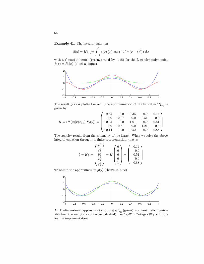
66
Example 41. The integral equation
g(y) = Kg |y=
∫ 1
−1
g(x)(15 exp (−10 ∗ (x− y)2)
)dx
with a Gaussian kernel (green, scaled by 1/15) for the Legendre polynomialf(x) = P4(x) (blue) as input:
−1 −0.8 −0.6 −0.4 −0.2 0 0.2 0.4 0.6 0.8 1−2
−1
0
1
2
The result g(x) is plotted in red. The approximation of the kernel in H4Leg is
given by
K = 〈Pi(x)|k(x, y)|Pj(y)〉 =
2.55 0.0 −0.35 0.0 −0.140.0 2.07 0.0 −0.51 0.0
−0.35 0.0 1.61 0.0 −0.510.0 −0.51 0.0 1.21 0.0
−0.14 0.0 −0.52 0.0 0.88
The sparsity results from the symmetry of the kernel. When we solve the aboveintegral equation through its finite representation, that is
g = Kg =
g5
1
g52
g53
g54
g55
= K
00001
=
−0.14
0.0−0.51
0.00.88
we obtain the approximation g(y) (shown in blue)
−1 −0.8 −0.6 −0.4 −0.2 0 0.2 0.4 0.6 0.8 1−2
−1
0
1
2
An 11-dimensional approximation g(y) ∈ H10Leg (green) is almost indistinguish-
able from the analytic solution (red, dashed). See legPlotIntegralEquation.mfor the implementation.
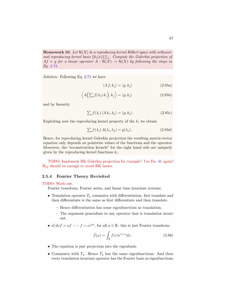
67
Homework 10. Let H(X) be a reproducing kernel Hilbert space with orthonor-mal reproducing kernel basis ki(x)∞i=1. Compute the Galerkin projection ofAf = g for a linear operator A : H(X) → H(X) by following the steps inEq. 2.71.
Solution: Following Eq. 2.71 we have
〈Af, kj〉 = 〈g, kj〉 (2.85a)⟨A(∑
if(λi) ki
), kj
⟩= 〈g, kj〉 (2.85b)
and by linearity ∑if(λi) 〈Aki, kj〉 = 〈g, kj〉 . (2.85c)
Exploiting now the reproducing kernel property of the ki we obtain∑if(λi)A(λi, λj) = g(λj). (2.85d)
Hence, for reproducing kernel Galerkin projection the resulting matrix-vectorequation only depends on pointwise values of the functions and the operator.Moreover, the “reconstruction kernels” for the right hand side are uniquelygiven by the reproducing kernel functions ki.
TODO: Implement RK Galerkin projection for example? Use Ex. 41 again?H10 should be enough to avoid RK issues.
2.5.4 Fourier Theory Revisited
TODO: Work out.Fourier transform, Fourier series, and linear time invariant systems.
• Translation operator Ta commutes with differentiation: first translate andthen differentiate is the same as first differentiate and then translate.
– Hence differentiation has some eigenfunctions as translation.– The argument generalizes to any operator that is translation invari-
ant.
• d/dxf = af => f = ceax, for all a ∈ R: this is just Fourier transform:
f(ω) =
∫Rf(x)ei ω xdx. (2.86)
• The equation is just projection into the eigenbasis.
• Commutes with Ta. Hence Ta has the same eigenfunctions. And thenevery translation invariant operator has the Fourier basis as eigenfunctions.
68
• Consequently, translation invariant operators are diagonalized by Fourierbasis.
• Application of operator is then multiplication by spectrum. Since R isnon-compact the spectrum is continuous and it means applying a functionto the continuous spectral representation.
• Spectrum is continuous for noncompact domain.
– This is why the basis expansion is an integral and not a sum.
• But is there an obvious reason why it is discrete on compact domains?
Remark 16. When X = Rn, then the Sobolev spaces W k,p(Rn) can also bedefined using the Fourier transform F as
W k,p(Rn) =f ∈ Lp(Rn) | F−1
((1 + ξ)k/2f
)∈ Lp(Rn)
, (2.87)
where f denotes the Fourier transform of the function f , that is f = F (f), andthe behaviour of the derivatives is controlled by the weight (1 + ξ)k/2 whichenforces a suitable decay of the Fourier coefficients as the frequency ξ goes toinfinity. The above definition can be extended from Rn to other domains wherea suitable generalization of the Fourier transform is defined, for example onthe sphere,28 and it also allows to introduce Sobolev spaces where k is not aninteger.
Remark 17. Mention Fourier and derivative -> symbol calculus.
Remark 18. Beyond Fourier many other integral transforms that might beuseful. For example, the Hilbert transform plays an essential role for therepresentation of wave signals.29
2.6 Further Reading
A comprehensive discussion of mathematical basis of signal processing can befound in the classic text by Mallat.30 Introductions to the theory of frames canbe found in the survey articles by Kovacevic and Chebira.31 Approximationtheory is very large subject in itself. A useful recent accounts on the classicaltheory is presented by Trefethen32 and a good starting point for the modern
28For Sobolev spaces over the sphere see for example (Freeden, Gervens, and Schreiner,Constructive Approximation on the Sphere (With Applications to Geomathematics); Hesse,“Complexity of numerical integration over spherical caps in a Sobolev space setting”).
29Mandel and Wolf, Optical Coherence and Quantum Optics, Chapter 3.30Mallat, A Wavelet Tour of Signal Processing: The Sparse Way.31Kovacevic and Chebira, “Life Beyond Bases: The Advent of Frames (Part I)”; Kovacevic
and Chebira, “Life Beyond Bases: The Advent of Frames (Part II)”.32(Trefethen, Approximation Theory and Approximation Practice), see also (Davis, Inter-
polation and Approximation; Cheney and Light, A Course in Approximation Theory).

69
theory for signals with varying regularity is again presented by Mallat.33 For amore rigorous and mathematical treatment of function spaces see for example theclassic text by Lax34 or the books by Rudin.35 For an alternative introductionto finite element methods see the article by Trenogin.36
33(Mallat, A Wavelet Tour of Signal Processing: The Sparse Way), see for examplealso (R. A. DeVore and Lorentz, Constructive approximation; R. A. DeVore, “Nonlinear Approx-imation”; Wendland, Scattered Data Approximation; Freeden, Gervens, and Schreiner, Con-structive Approximation on the Sphere (With Applications to Geomathematics); Temlyakov,“Nonlinear Methods of Approximation”; Reimer, Multivariate Polynomial Approximation;Cucker and Zhou, Learning Theory: An Approximation Theory Viewpoint).
34Lax, Functional Analysis.35Rudin, Principles of Mathematical Analysis; Rudin, Real and Complex Analysis; Rudin,
Functional Analysis.36Trenogin, “Galerkin Method”.

Chapter 3
Manifolds and Tensors
Relevance for graphics: - Meshes, as discussed in more detail in the next section.- For simulation. - For manifold learning, i.e. the analysis of high dimen-sional data.1 - Lie groups: Rotations are omnipresent in graphics, symmetrydetection,2 Lie group integrators.3
3.1 Preliminaries
In the following, it will be useful to have in mind some notions from algebraabout the relationship between mathematical structures. We will thereforerecall them at this point.
Definition 3.1. A homomorphism is a structure preserving map betweenalgebraic structures.
Homomorphisms exists for different structures, such as algebras, Lie algebras,rings, and groups, and the precise meaning of the term depends on the structureof interest. The following examples demonstrate this.
Example 42. Let (H(X), 〈 , 〉) be a finite dimensional Hilbert space, and letϕini=1 and orthonormal basis for H(X). Then ϕini=1 defines a Hilbert spacehomomorphism from H(X) to Rn with the usual Euclidean inner product.
1(Coifman, Lafon, Lee, Maggioni, Nadler, Warner, and Zucker, “Geometric Diffusions as aTool for Harmonic Analysis and Structure Definition of Data: Diffusion Maps”; Coifman, Lafon,Lee, Maggioni, Nadler, Warner, and Zucker, “Geometric Diffusions as a Tool for HarmonicAnalysis and Structure Definition of Data: Multiscale Methods”) and references therein. Apivotal early paper is those by Belin and Niyogi (“Laplacian Eigenmaps for DimensionalityReduction and Data Representation”).
2(Lipman, Chen, Daubechies, and Funkhouser, “Symmetry Factored Embedding andDistance”); through the intimate relationship between rotations and the Laplace operatoralso methods that employ spherical harmonics can be considered to be based on Lie groups,see e.g. (Kazhdan, Funkhouser, and Rusinkiewicz, “Rotation Invariant Spherical HarmonicRepresentation of 3D Shape Descriptors”).
3Kobilarov, Crane, and Desbrun, “Lie Group Integrators for Animation and Control ofVehicles”.
71
72
This is just a more formal version of the previous observation that, using anorthonormal basis such as ϕini=1, all operations in H(X) can equivalently beperformed in Rn.
Example 43. A Lie algebra homomorphism ϕ : (g, [ , ]g) → (h, [ , ]h) be-tween two Lie algebras (g, [ , ]g) and (h, [ , ]h) is a map such that [X,Y ]g =[ϕ(X), ϕ(Y )]h for all X,Y ∈ g.
Definition 3.2. An isomorphism between two algebraic structures is a ho-momorphism whose inverse is also a homomorphism.
An isomorphism thus defines an equivalence between two structures that enablesto perform all operations on the first structure also with the second one, andthen relate the result back to the first. When two structures A and B areisomorphic then this will be denoted as A ∼= B.
Example 44. Extending Example 42, any finite dimensional Hilbert space(H, 〈 , 〉) of dimension n is isomorphic to Euclidean space (Rn, ·) with the innerproduct over H being the dot product over Rn.
Definition 3.3. An endomorphism is a homomorphism from an object ontoitself.
Definition 3.4. An automorphism is an isomorphism from an object ontoitself.
Automorphisms are for example of importance in the context of (Lie) groupswhen it is acting on itself.
Definition 3.5. A homeomorphism ϕ : S → T between topological spaces Sand T is a bijective mapping that is continuous and has a continuous inverse.
By the required continuity, a homeomorphism is an isomorphism in the cate-gory of topological spaces, preserving the topological structure of S and T . Somecare is required to distinguish homomorphisms and homeomorphisms whichare related—and orthographically almost coincide—but nonetheless distinctconcepts.
3.2 Manifolds
3.2.1 Continuous Theory
3.2.2 Discrete Theory
3.3 Tensors
Distinguish from the tensors, that is multi-dimensional arrays, that sometimesappear in computer science.4 - The connection is that the representation of thetensors we talk about can be multi-linear arrays.
4Vasilescu and Terzopoulos, “TensorTextures”; Vasilescu and Terzopoulos, “MultilinearAnalysis of Image Ensembles: TensorFaces”; Tsai and Shih, “All-Frequency Precomputed Radi-
73
Exercises: Derivatives for matrices.
3.4 Differential Forms and Exterior Calculus
3.4.1 Continuous Theory
Use integration as example application. Also the crucial aspect for discretization.Remark on Lp spaces on manifolds.
3.4.2 Discrete Theory
3.5 The Lie Derivative
Develop continuous theory.Make some remarks on discrete theory but no well developed theory so far.
3.6 Riemannian Manifolds
3.6.1 Continuous Theory
3.6.2 Discrete Theory
3.7 Lie Groups
Also talk about representations of matrices: this is how they occur almostalways in applications.
For the examples build on the material in Mechanics and Symmetry.
3.7.1 The Euclidean Group
In Example 7 we already showed that a linear space has a group structure.
3.7.2 The Rotation Group
SO(3) and its different realizations (including quaternions) as example.
3.7.3 Diffeomorphism Groups
3.8 Further Reading
A comprehensive and rigorous discussion of manifolds and tensor calculus canbe found in the book by Marsden, Ratiu, and Abraham.5 A shorter introductioncan be found in the “little Spivak”.6 A classical presentation from the point of
ance Transfer Using Spherical Radial Basis Functions and Clustered Tensor Approximation”.5Marsden, Ratiu, and Abraham, Manifolds, Tensor Analysis, and Applications.6Spivak, Calculus on Manifolds: A Modern Approach to Classical Theorems of Advanced
Calculus.

74
physics that also tries to provide as much intuition as possible is those in the“Big Black Book: B3” by Misner, Thorne, and Wheeler.7
7Misner, Thorne, and Wheeler, Gravitation.
Chapter 4
Dynamical Systems and GeometricMechanics
- Simulation and animation; although so far almost exclusively used for simula-tion and control. - Fluid simulation.1 - Control.2 - Elastics.3.
4.1 Motivation and Intuition
4.2 Ordinary and Partial Differential Equations
4.3 Hamiltonian Mechanics
4.3.1 Continuous Theory
Example 45. Method of characteristics, at least for f = −f,H.
4.3.2 Symplectic Integrators
4.4 Lagrangian Mechanics
4.4.1 Continuous Theory
Remark 19 (Calculus of Variations). Explain basic rules of classical classicalcalculus of variations.
1Elcott, Tong, Kanso, Schröder, and Desbrun, “Stable, Circulation-Preserving, SimplicialFluids”; Pavlov, Mullen, Tong, Kanso, Marsden, and Desbrun, “Structure-preserving discretiza-tion of incompressible fluids”; Mullen, Crane, Pavlov, Tong, and Desbrun, “Energy-PreservingIntegrators for Fluid Animation”.
2Kobilarov, Crane, and Desbrun, “Lie Group Integrators for Animation and Control ofVehicles”.
3Bergou, Wardetzky, Robinson, Audoly, and Grinspun, “Discrete Elastic Rods”; Bergou,Audoly, Vouga, Wardetzky, and Grinspun, “Discrete Viscous Threads”; Batty, Uribe, Audoly,and Grinspun, “Discrete Viscous Sheets”.
75
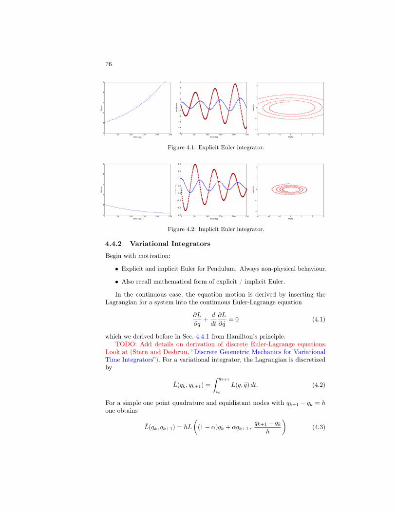
76
0 50 100 150 200 250time step
0
1
2
3
4
5
Energ
y
0 50 100 150 200 250time step
5
4
3
2
1
0
1
2
3
4
am
plit
ude
3 2 1 0 1 2 3theta
2
1
0
1
2
velo
city
Figure 4.1: Explicit Euler integrator.
0 50 100 150 200 250time step
0
1
2
3
4
5
Energ
y
0 50 100 150 200 250time step
2.0
1.5
1.0
0.5
0.0
0.5
1.0
1.5
am
plit
ude
3 2 1 0 1 2 3theta
2
1
0
1
2
velo
city
Figure 4.2: Implicit Euler integrator.
4.4.2 Variational Integrators
Begin with motivation:
• Explicit and implicit Euler for Pendulum. Always non-physical behaviour.
• Also recall mathematical form of explicit / implicit Euler.
In the continuous case, the equation motion is derived by inserting theLagrangian for a system into the continuous Euler-Lagrange equation
∂L
∂q+d
dt
∂L
∂q= 0 (4.1)
which we derived before in Sec. 4.4.1 from Hamilton’s principle.TODO: Add details on derivation of discrete Euler-Lagrange equations.
Look at (Stern and Desbrun, “Discrete Geometric Mechanics for VariationalTime Integrators”). For a variational integrator, the Lagrangian is discretizedby
L(qk, qk+1) =
∫ qk+1
tk
L(q, q) dt. (4.2)
For a simple one point quadrature and equidistant nodes with qk+1 − qk = hone obtains
L(qk, qk+1) = hL
((1− α)qk + αqk+1 ,
qk+1 − qkh
)(4.3)
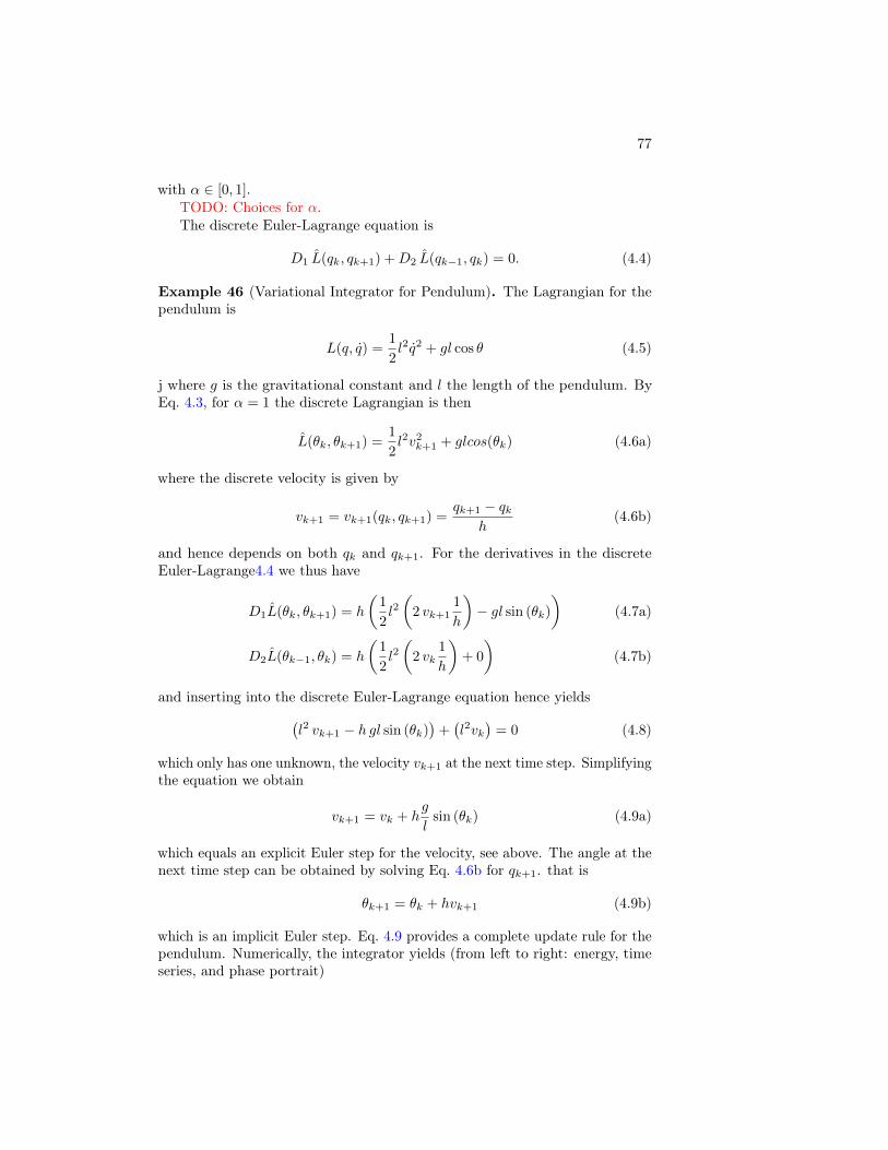
77
with α ∈ [0, 1].TODO: Choices for α.The discrete Euler-Lagrange equation is
D1 L(qk, qk+1) +D2 L(qk−1, qk) = 0. (4.4)
Example 46 (Variational Integrator for Pendulum). The Lagrangian for thependulum is
L(q, q) =1
2l2q2 + gl cos θ (4.5)
j where g is the gravitational constant and l the length of the pendulum. ByEq. 4.3, for α = 1 the discrete Lagrangian is then
L(θk, θk+1) =1
2l2v2
k+1 + glcos(θk) (4.6a)
where the discrete velocity is given by
vk+1 = vk+1(qk, qk+1) =qk+1 − qk
h(4.6b)
and hence depends on both qk and qk+1. For the derivatives in the discreteEuler-Lagrange4.4 we thus have
D1L(θk, θk+1) = h
(1
2l2(
2 vk+11
h
)− gl sin (θk)
)(4.7a)
D2L(θk−1, θk) = h
(1
2l2(
2 vk1
h
)+ 0
)(4.7b)
and inserting into the discrete Euler-Lagrange equation hence yields(l2 vk+1 − h gl sin (θk)
)+(l2vk
)= 0 (4.8)
which only has one unknown, the velocity vk+1 at the next time step. Simplifyingthe equation we obtain
vk+1 = vk + hg
lsin (θk) (4.9a)
which equals an explicit Euler step for the velocity, see above. The angle at thenext time step can be obtained by solving Eq. 4.6b for qk+1. that is
θk+1 = θk + hvk+1 (4.9b)
which is an implicit Euler step. Eq. 4.9 provides a complete update rule for thependulum. Numerically, the integrator yields (from left to right: energy, timeseries, and phase portrait)
78
0 50 100 150 200 250time step
0
1
2
3
4
5
Energ
y
0 50 100 150 200 250time step
2.0
1.5
1.0
0.5
0.0
0.5
1.0
1.5
2.0
am
plit
ude
3 2 1 0 1 2 3theta
2
1
0
1
2
velo
city
and, in contrast to the explicit and implict Euler integrator in Fig. 4.1 andFig. 4.2, we obtain a qualitatively correct harmonic motion. Note that Eq. 4.9differs from the formulas for the explicit and implicit Euler schemes only slightly,but with a tremendous difference in the numerics. Also the computation is notmore expensive than an explicit Euler-Integrator, the simplest possible scheme,while the nonlinear solve that is needed for the implicit Euler-scheme is avoided.
4.5 Symmetries
4.6 Further Reading
Books on geometric mechanics are for example the classic texts by Abrahamand Marsden4 and Arnold5. More current treatments can be found in booksby Marsden and Ratiu,6 which discusses a wealth of physical systems, and thebooks by Holm and co-workers7 that provide a more pedagogical exposition.
4Abraham and Marsden, Foundations of Mechanics.5Arnold, Mathematical Methods of Classical Mechanics.6Marsden and Ratiu, Introduction to Mechanics and Symmetry: A Basic Exposition of
Classical Mechanical Systems.7Holm, Geometric Mechanics: Dynamics and Symmetry; Holm, Geometric mechanics:
Rotating, translating and rolling; Holm, Schmah, and Stoica, Geometric Mechanics andSymmetry: From Finite to Infinite Dimensions.


Bibliography
Abraham, R. and J. E. Marsden. Foundations of Mechanics. second. Addison-Wesley Pub-lishing Company, Inc., 1978. url: http://caltechbook.library.caltech.edu/103/.
Arnold, V. I. Mathematical Methods of Classical Mechanics. second. Graduate Texts inMathematics. Springer, Sept. 1989.
Batty, C., A. Uribe, B. Audoly, and E. Grinspun. “Discrete Viscous Sheets”. In: ACMTransactions on Graphics 31.4 (July 2012), pp. 1–7. url: http://dl.acm.org/citation.cfm?id=2185520.2185609.
Belkin, M. and P. Niyogi. “Laplacian Eigenmaps for Dimensionality Reduction and DataRepresentation”. en. In: Neural Computation 15.6 (June 2003), pp. 1373–1396. url: http://www.mitpressjournals.org/doi/abs/10.1162/089976603321780317?journalCode=neco.
Bellman, R. Adaptive Control Processes: A Guided Tour. Princeton University Press, 1966.
Bergou, M., B. Audoly, E. Vouga, M. Wardetzky, and E. Grinspun. “Discrete Viscous Threads”.In: ACM Transactions on Graphics 29.4 (July 2010), p. 1. url: http://dl.acm.org/citation.cfm?id=1778765.1778853.
Bergou, M., M. Wardetzky, S. Robinson, B. Audoly, and E. Grinspun. “Discrete Elastic Rods”.In: ACM SIGGRAPH 2008 papers on - SIGGRAPH ’08. Vol. 27. 3. New York, NewYork, USA: ACM Press, Aug. 2008, p. 1. url: http://dl.acm.org/citation.cfm?id=1399504.1360662.
Botsch, M., L. Kobbelt, M. Pauly, P. Alliez, and B. Levy. Polygon Mesh Processing. A KPeters/CRC Press, 2010. url: http://www.amazon.com/Polygon-Mesh-Processing-Mario-Botsch/dp/1568814267.
Bungartz, H.-J. and M. Griebel. “Sparse Grids”. In: Acta Numerica 13 (May 2004), pp. 147–269. url: http://journals.cambridge.org/abstract\_S0962492904000182.
Candès, E. J. and B. Recht. “Exact Matrix Completion via Convex Optimization”. In:Foundations of Computational Mathematics 9.6 (Apr. 2009), pp. 717–772. url: http://link.springer.com/10.1007/s10208-009-9045-5.
Candès, E. J., J. Romberg, and T. Tao. “Robust Uncertainty Principles: Exact Signal Recon-struction from Highly Incomplete Frequency Information”. In: Information Theory, IEEETransactions on 52 (2006), pp. 489–509. url: http://dx.doi.org/10.1109/TIT.2005.862083.
Candès, E. J. and M. B. Wakin. “An Introduction to Compressive Sampling”. In: SignalProcessing Magazine, IEEE 25 (2008), pp. 21–30. url: http://dx.doi.org/10.1109/MSP.2007.914731.
Cheney, E. W. and W. A. Light. A Course in Approximation Theory. AMS Bookstore, 2009.
Chenney, S. and D. A. Forsyth. “Sampling Plausible Solutions to Multi-body ConstraintProblems”. In: Proceedings of the 27th annual conference on Computer graphics and
81
82
interactive techniques - SIGGRAPH ’00. New York, New York, USA: ACM Press, July2000, pp. 219–228. url: http://dl.acm.org/citation.cfm?id=344779.344882.
Christensen, P. H. “Adjoints and Importance in Rendering: an Overview”. In: IEEE Transac-tions on Visualization and Computer Graphics 9 (2003), pp. 329–340.
Coifman, R. R., S. Lafon, A. B. Lee, M. Maggioni, B. Nadler, F. Warner, and S. W. Zucker.“Geometric Diffusions as a Tool for Harmonic Analysis and Structure Definition of Data:Diffusion Maps”. In: Proceedings of the National Academy of Sciences of the United Statesof America 102 (2005), pp. 7426–7431. url: http://www.pnas.org/content/102/21/7426.abstract.
— “Geometric Diffusions as a Tool for Harmonic Analysis and Structure Definition of Data:Multiscale Methods”. In: Proceedings of the National Academy of Sciences of the UnitedStates of America 102 (2005), pp. 7432–7437. url: http://www.pnas.org/content/102/21/7432.abstract.
Cucker, F. and D.-X. Zhou. Learning Theory: An Approximation Theory Viewpoint. Cam-bridge Monographs on Applied and Computational Mathematics. Cambridge UniversityPress, 2007.
Davis, P. J. Interpolation and Approximation. Dover books on advanced mathematics. DoverPublications, 1975.
DeVore, R. Capturing Functions in High Dimensions. Tech. rep. Paris: Course Notes, 2009.
DeVore, R. A. “Nonlinear Approximation”. In: Acta Numerica 7 (Jan. 1998), pp. 51–150. url:http://journals.cambridge.org/abstract\_S0962492900002816.
DeVore, R. A. and G. G. Lorentz. Constructive approximation. Springer, 1993. url: http://books.google.com/books?id=cDqNW6k7\_ZwC\&pgis=1.
Dick, J. and F. Pillichshammer. Digital Nets and Sequences: Discrepancy Theory and Quasi-Monte Carlo Integration. Cambridge University Press, 2010.
Donoho, D. L. “Compressed Sensing”. In: IEEE Transactions on Information Theory 52(2006), pp. 1289–1306.
— “High-Dimensional Data Analysis: The Curses and Blessings of Dimensionality”. In: Math-ematical Challenges of the 21st Century. Los Angeles, CA, USA: American MathematicalSociety, 2000. url: http://www-stat.stanford.edu/~donoho/Lectures/CBMS/Curses.pdf.
Donoho, D. L., A. Maleki, I. U. Rahman, M. Shahram, and V. Stodden. “Reproducible Researchin Computational Harmonic Analysis”. In: Computing in Science and Engineering 11.1(2009), pp. 8–18.
Elcott, S., Y. Tong, E. Kanso, P. Schröder, and M. Desbrun. “Stable, Circulation-Preserving,Simplicial Fluids”. In: ACM Transactions on Graphics 26.1 (2007).
Finkelstein, A. and D. H. Salesin. “Multiresolution Curves”. In: SIGGRAPH ’94: Proceedings ofthe 21st annual Conference on Computer Graphics and Interactive Techniques.New York, NY, USA: ACM Press, 1994, pp. 261–268.
Freeden, W., T. Gervens, and M. Schreiner. Constructive Approximation on the Sphere (WithApplications to Geomathematics). Oxford Sciences Publication. Clarendon Press, OxfordUniversity, 1998.
Galerkin, B. G. “On Electrical Circuits for the Approximate Solution of the Laplace Equation”.Russian. In: Vestnik Inzh. 19 (1915), pp. 897–908.
Golub, G. H. and C. F. Van Loan. Matrix Computations. Johns Hopkins Studies in Mathe-matical Sciences. The Johns Hopkins University Press, 1996.
83
Gortler, S. J., P. Schröder, M. F. Cohen, and P. Hanrahan. “Wavelet Radiosity”. In: Com-puter Graphics Proceedings, Annual Conference Series, 1993 (ACM SIGGRAPH ’93Proceedings). 1993, pp. 221–230.
Grinstead, Charles M and J Laurie Snell. Introduction to Probability. American MathematicalSociety, 2006.
Hesse, K. “Complexity of numerical integration over spherical caps in a Sobolev space setting”.In: Journal of Complexity In press (Sept. 2010). url: http://dx.doi.org/10.1016/j.jco.2010.09.002.
Holm, D. D. Geometric Mechanics: Dynamics and Symmetry. Vol. Part I. London: ImperialCollege Press, 2008.
— Geometric mechanics: Rotating, translating and rolling. Vol. II. Imperial College Press,2008.
Holm, D. D., T. Schmah, and C. Stoica. Geometric Mechanics and Symmetry: From Finiteto Infinite Dimensions. Oxford texts in applied and engineering mathematics. OxfordUniversity Press, 2009, 515 p.
Horn, R. A. and C. R. Johnson. Matrix Analysis. Cambridge University Press, 1990.
Kazhdan, M., T. Funkhouser, and S. Rusinkiewicz. “Rotation Invariant Spherical HarmonicRepresentation of 3D Shape Descriptors”. In: ACM International Conference ProceedingSeries; Vol. 43 (2003). url: http://portal.acm.org/citation.cfm?id=882370.882392.
Kobilarov, M., K. Crane, and M. Desbrun. “Lie Group Integrators for Animation and Controlof Vehicles”. In: ACM Transactions on Graphics (TOG) 28.2 (2009). url: http://portal.acm.org/citation.cfm?id=1516522.1516527.
Kovacevic, J. and A. Chebira. “Life Beyond Bases: The Advent of Frames (Part I)”. In: SignalProcessing Magazine, IEEE 24.4 (2007), pp. 86 –104. url: http://ieeexplore.ieee.org/xpl/freeabs\_all.jsp?arnumber=4286567.
— “Life Beyond Bases: The Advent of Frames (Part II)”. In: IEEE Signal Processing Magazine24.5 (2007), pp. 115–125. url: http://ieeexplore.ieee.org/lpdocs/epic03/wrapper.htm?arnumber=4350231.
Lax, P. D. Functional Analysis. New York: Wiley-Interscience, 2002.
— Linear Algebra and Its Applications. second ed. Pure and Applied Mathematics. WileyInterscience, 2007.
Lax, P. D. and A. N. Milgram. “Parabolic equations”. In: Contributions to the theory ofpartial differential equations. Annals of Mathematics Studies. Princeton, N. J.: PrincetonUniversity Press, 1954, pp. 167–190.
Lehtinen, J. “A Framework for Precomputed and Captured Light Transport”. In: ACM Trans.Graph. 26 (2007), p. 13.
Lehtinen, J., M. Zwicker, E. Turquin, J. Kontkanen, F. Durand, F. X. Sillion, and T. Aila. “AMeshless Hierarchical Representation for Light Transport”. In: ACM Trans. Graph. 27(2008), pp. 1–9.
Lessig, C. “Modern Foundations of Light Transport Simulation”. Ph.D. thesis. Toronto: Uni-versity of Toronto, 2012. url: http://users.cms.caltech.edu/~lessig/dissertation/lessig\_dissertation.pdf.
Lipman, Y., X. Chen, I. Daubechies, and T. Funkhouser. “Symmetry Factored Embeddingand Distance”. In: ACM SIGGRAPH 2010 papers on - SIGGRAPH ’10. Vol. 29. 4. NewYork, New York, USA: ACM Press, July 2010, p. 1. url: http://dl.acm.org/citation.cfm?id=1833349.1778840.
Mallat, S. G. A Wavelet Tour of Signal Processing: The Sparse Way. third ed. AcademicPress, 2009.
84
Mandel, L. and E. Wolf. Optical Coherence and Quantum Optics. Cambridge, UK: CambridgeUniversity Press, Sept. 1995.
Marsden, J. E. and T. S. Ratiu. Introduction to Mechanics and Symmetry: A Basic Expositionof Classical Mechanical Systems. third ed. Texts in Applied Mathematics. New York:Springer-Verlag.
Marsden, J. E., T. S. Ratiu, and R. Abraham. Manifolds, Tensor Analysis, and Applications.third. Applied Mathematical Sciences. New York: Springer-Verlag, 2004.
Misner, C. W., K. S. Thorne, and J. A. Wheeler. Gravitation. San Francisco, CA, USA: W.H. Freeman, 1973.
Mitchell, D. P. “Spectrally Optimal Sampling for Distribution Ray Tracing”. In: SIGGRAPHComput. Graph. 25 (1991), pp. 157–164.
Mullen, P., K. Crane, D. Pavlov, Y. Tong, and M. Desbrun. “Energy-Preserving Integratorsfor Fluid Animation”. In: ACM Transactions on Graphics (Proceedings of SIGGRAPH2009) 28.3 (2009), pp. 1–8.
Öztireli, A. C., M. Alexa, and M. Gross. “Spectral Sampling of Manifolds”. In: ACM Transac-tions on Graphics (Proceedings of SIGGRAPH Asia 2010) 29.6 (Dec. 2010), p. 1. url:http://dl.acm.org/citation.cfm?id=1882262.1866190.
Pavlov, D., P. Mullen, Y. Tong, E. Kanso, J. E. Marsden, and M. Desbrun. “Structure-preserving discretization of incompressible fluids”. In: Physica D: Nonlinear Phenomena240.6 (Mar. 2011), pp. 443–458. url: http://dx.doi.org/10.1016/j.physd.2010.10.012.
Petrov, G. I. “Application of the Method of Galerkin to a Problem Involving the StationaryFlow of a Viscous Fluid”. In: Prikl. Matem. Mekh. 4.3 (1940).
Press, W. H., S. A. Teukolsky, W. T. Vetterling, and B. P. Flannery. Numerical Recipes inC: The Art of Scientific Computing. New York, NY, USA: Cambridge University Press,1992.
Ramamoorthi, R. “Precomputation-Based Rendering”. In: Foundations and Trends in Com-puter Graphics and Vision 3.4 (2007), pp. 281–369.
Reimer, M. Multivariate Polynomial Approximation. International Series of Numerical Math-ematics. Basel: Birkhäuser Verlag, 2003.
Rudin, W. Functional Analysis. International Series in Pure and Applied Mathematics. NewYork: McGraw-Hill Inc., 1991.
— Principles of Mathematical Analysis. International Series in Pure & Applied Mathematics.McGraw-Hill Publishing Co., Sept. 1976.
— Real and Complex Analysis. McGraw-Hill International Editions: Mathematics Series.McGraw-Hill Education - Europe, Mar. 1987.
Schröder, P., S. J. Gortler, M. F. Cohen, and P. Hanrahan. “Wavelet Projections for Radiosity”.In: Fourth Eurographics Workshop on Rendering. Paris, France, June 1993, pp. 105–114.
Schröder, P. and W. Sweldens. “Spherical Wavelets: Efficiently Representing Functions on theSphere”. In: Proceedings of ACM SIGGRAPH 1995. New York, NY, USA: ACM Press,1995, pp. 161–172.
— “Spherical Wavelets: Texture Processing”. In: Rendering Techniques ’95. Ed. by P Hanra-han and W Purgathofer. Wien, New York: Springer Verlag, Aug. 1995, pp. 252–263.
Sorkine, O. “Laplacian Mesh Processing”. In: Eurographics 2005, State of the Art Reports.2005, pp. 53–70.
Spivak, M. Calculus on Manifolds: A Modern Approach to Classical Theorems of AdvancedCalculus. HarperCollins Publishers, 1971.
85
Stakgold, I. and M. J. Holst. Green’s Functions and Boundary Value Problems. third ed.Pure and Applied Mathematics. John Wiley \& Sons, Inc., 2011.
Stern, A. and M. Desbrun. “Discrete Geometric Mechanics for Variational Time Integrators”.In: SIGGRAPH ’06: ACM SIGGRAPH 2006 Courses. ACM, 2006. url: http://portal.acm.org/citation.cfm?id=1185657.1185669.
Taubin, G. “A Signal Processing Approach to Fair Surface Design”. In: Proceedings of the22nd annual conference on Computer graphics and interactive techniques - SIGGRAPH’95. New York, New York, USA: ACM Press, Sept. 1995, pp. 351–358. url: http://dl.acm.org/citation.cfm?id=218380.218473.
Temlyakov, V. N. “Nonlinear Methods of Approximation”. In: Foundations of ComputationalMathematics 3.1 (Jan. 2003), pp. 33–107. url: http://link.springer.com/10.1007/s102080010029.
Trefethen, L. N. Approximation Theory and Approximation Practice. Society for Industrialand Applied Mathematics, 2012.
Trenogin, V. A. “Galerkin Method”. In: Encyclopedia of Mathematics. Ed. by M. Hazewinkel.Kluwer Academic Publishers, 2002. url: http://www.encyclopediaofmath.org/index.php?title=Galerkin\_method\&oldid=16286.
Tsai, Yu-Ting and Zen-Chung Shih. “All-Frequency Precomputed Radiance Transfer UsingSpherical Radial Basis Functions and Clustered Tensor Approximation”. In: Transactionsof Graphics (Proceedings of Siggraph 2006) 25.3 (Proceedings of ACM SIGGRAPH 2006)(2006). url: http://portal.acm.org/citation.cfm?id=1179352.1141981.
Vasilescu, M. A. O. and D. Terzopoulos. “Multilinear Analysis of Image Ensembles: Ten-sorFaces”. In: Computer Vision-ECCV 2002. Ed. by Anders Heyden, Gunnar Sparr,Mads Nielsen, and Peter Johansen. Vol. 2350. Lecture Notes in Computer Science. Berlin,Heidelberg: Springer, Apr. 2006. url: http://www.springerlink.com/index/10.1007/3-540-47969-4.
— “TensorTextures”. In: ACM Transactions on Graphics 23.3 (Aug. 2004), p. 336. url:http://dl.acm.org/citation.cfm?id=1015706.1015725.
Veach, E. and L. J. Guibas. “Metropolis Light Transport”. In: SIGGRAPH ’97: Proceedings ofthe 24th annual conference on computer graphics and interactive techniques. New York,NY, USA: ACM Press/Addison-Wesley Publishing Co., 1997, pp. 65–76.
Wendland, H. Scattered Data Approximation. Cambridge monographs on applied and compu-tational mathematics. Cambridge University Press, 2005.
Zatz, H. R. “Galerkin Radiosity: A Higher Order Solution Method for Global Illumination”.In: International Conference on Computer Graphics and Interactive Techniques (1993).url: http://portal.acm.org/citation.cfm?id=166145.

Index
SymbolsLp space, 27
AAbelian group, 21adjoint of a linear map, 7affine, 22affine space, 22automorphism, 72
Bboundary condition, 54boundary conditions
Dirichlet, 54Neumann, 54
Ccalculus of variations, 75characteristic basis, 48characteristic function, 48circulant matrix, 13composition of linear maps, 3compressed sensing, 38curse of dimensionality, 39
Ddiagonal matrix, 13diagonalization of a linear map, 14differential operator
nonlinear, 57Dirac delta, 41Dirichlet boundary conditions, 54distribution in the sense of Schwartz, 41domain of a linear map, 3
Eeigenvalue of a linear map, 11eigenvector of a linear map, 11endomorphism, 72Euler equation, 57Euler-Lagrange equation
discrete, 77
Ffinite element method
mass matrix, 64stiffness matrix, 64
finite element methods, 62function, 25function space, 26
GGalerkin projection, 61generalized function, 41Green’s function, 60
eigenvector expansion, 60group, 20
Abelian, 21identity element, 21inverse element, 21permutation, 21
Hheat equation, 55Hilbert-Schmidt integral operator, 57Hilbert-Sobolev space, 30homeomorphism, 72homomorphism, 71Hölder exponent, 37Hölder orm, 37
Iidentity map, 3identity operator
integral representation, 58image of linear map, 4integral operator, 57
Markov chain, 58nonlinear, 59
inverse of a linear map, 6isomorphism, 72
Kkernel of linear map, 4
87
88
Kolmogorov width, 39
LLaplace equation, 60Laplace operator, 54Lebesgue space, 27
L2, 29Lie group, 20linear least squares, 17
normal equation, 18linear map, 2
adjoint, 7diagonalization, 14domain, 3eigenvalue, 11eigenvector, 11image, 4inverse, 6kernel, 4orthogonal, 8pseudo inverse, 7range, 4rank, 4self-adjoint, 7singular value decomposition, 15target, 3unitary, 8
linear mapscomposition, 3vector space structure, 11
linear operator, 51linear space
group structure, 21Lipschitz regularity, 37low discrepancy sequence, 46
MMarkov chain, 58Markov process, 59mass matrix, 64matrix
orthogonal, 9Mercedes Benz frame, 2
generalization to 3D, 2method of characteristics, 75Moore-Penrose pseudo inverse, 7, 17
NNeumann boundary conditions, 54nonlinear operator
differential, 57integral, 59
normal equation for linear least squares,18
Oorthogonal linear map, 8orthogonal matrix, 9
PPaley-Wiener space, 42partial differential equation, 51partition, 48permutation
even, 21group, 21odd, 21sign, 21transposition, 21
point evaluation functional, 41Poisson equation, 60
spectral method, 64pseudo inverse of linear map, 7
Qquasi random points, 46
Rrange of linear operator, 4rank of a linear map, 4rank-nullity theorem, 4reproducing kernel, 42reproducing kernel Hilbert space, 42
SSchwartz kernel theorem, 58self-adjoint linear map, 7self-adjoint operator
spectral theorem, 12shift operator, 3signal, 25singular value decomposition, 15Sobolev space, 28, 30spectral methods, 64stationary solution, 55steady state, 55steady state distribution, 58stiffness matrix, 64
Ttarget of a linear map, 3test function, 41
Uunitary linear map, 8
Vvariation of a function, 28
space of, 28
Wwave equation, 56weak derivatives, 41

“My work always tried to unitethe truth with the beautiful,but when I had to chooseone or the other,I usually chose the beautiful.”
Hermann Weyl

© Christian Lessig 2014