Formula Book

for

Hydraulics and Pneumatics

Fluid and Mechanical Engineering Systems

Department of Management and Engineering

Linkoping University

Revised 2008-10-27

Contents

1 Elementary Equations 11.1 Nomenclature . . . . . . . . . . . . . . . . . . . . . . . . . . . . . . . . . . . . . . . 11.2 The continuity equation . . . . . . . . . . . . . . . . . . . . . . . . . . . . . . . . . 11.3 Reynolds number . . . . . . . . . . . . . . . . . . . . . . . . . . . . . . . . . . . . . 11.4 Flow equations . . . . . . . . . . . . . . . . . . . . . . . . . . . . . . . . . . . . . . 1

2 Pipe flow 22.1 Nomenclature . . . . . . . . . . . . . . . . . . . . . . . . . . . . . . . . . . . . . . . 22.2 Bernoullis extended equation . . . . . . . . . . . . . . . . . . . . . . . . . . . . . . 22.3 The flow loss, ∆pf . . . . . . . . . . . . . . . . . . . . . . . . . . . . . . . . . . . . 22.4 The friction factor, λ . . . . . . . . . . . . . . . . . . . . . . . . . . . . . . . . . . . 22.5 Disturbance source factor, ζs . . . . . . . . . . . . . . . . . . . . . . . . . . . . . . 22.6 Single loss factor, ζ . . . . . . . . . . . . . . . . . . . . . . . . . . . . . . . . . . . . 3

3 Orifices 63.1 Nomenclature . . . . . . . . . . . . . . . . . . . . . . . . . . . . . . . . . . . . . . . 63.2 The flow coefficient, Cq . . . . . . . . . . . . . . . . . . . . . . . . . . . . . . . . . 63.3 Series connection of turbulent orifices . . . . . . . . . . . . . . . . . . . . . . . . . . 63.4 Parallel connection of turbulent orifices . . . . . . . . . . . . . . . . . . . . . . . . 7

4 Flow forces 84.1 Nomenclature . . . . . . . . . . . . . . . . . . . . . . . . . . . . . . . . . . . . . . . 84.2 Spool . . . . . . . . . . . . . . . . . . . . . . . . . . . . . . . . . . . . . . . . . . . 8

5 Rotational transmissions 95.1 Nomenclature . . . . . . . . . . . . . . . . . . . . . . . . . . . . . . . . . . . . . . . 95.2 Efficiency models . . . . . . . . . . . . . . . . . . . . . . . . . . . . . . . . . . . . . 9

6 Accumulators 106.1 Nomenclature . . . . . . . . . . . . . . . . . . . . . . . . . . . . . . . . . . . . . . . 106.2 Calculating of the accumulator volume, V0 . . . . . . . . . . . . . . . . . . . . . . . 10

7 Gap theory 117.1 Nomenclature . . . . . . . . . . . . . . . . . . . . . . . . . . . . . . . . . . . . . . . 117.2 Plane parallel gap . . . . . . . . . . . . . . . . . . . . . . . . . . . . . . . . . . . . 117.3 Radial gap . . . . . . . . . . . . . . . . . . . . . . . . . . . . . . . . . . . . . . . . . 117.4 Gap between cylindrical piston and cylinder . . . . . . . . . . . . . . . . . . . . . . 117.5 Axial, annular gap . . . . . . . . . . . . . . . . . . . . . . . . . . . . . . . . . . . . 12

8 Hydrostatic bearings 138.1 Nomenclature . . . . . . . . . . . . . . . . . . . . . . . . . . . . . . . . . . . . . . . 138.2 Circled block . . . . . . . . . . . . . . . . . . . . . . . . . . . . . . . . . . . . . . . 138.3 Rectangular block . . . . . . . . . . . . . . . . . . . . . . . . . . . . . . . . . . . . 14

9 Hydrodynamic bearing theory 159.1 Nomenclature . . . . . . . . . . . . . . . . . . . . . . . . . . . . . . . . . . . . . . . 159.2 Cartesian coordinate . . . . . . . . . . . . . . . . . . . . . . . . . . . . . . . . . . . 159.3 Polar coordinates . . . . . . . . . . . . . . . . . . . . . . . . . . . . . . . . . . . . . 15

10 Non-stationary flow 1710.1 Nomenclature . . . . . . . . . . . . . . . . . . . . . . . . . . . . . . . . . . . . . . . 1710.2 Joukowskis equation . . . . . . . . . . . . . . . . . . . . . . . . . . . . . . . . . . . 1710.3 Retardation of cylinder with inertia load . . . . . . . . . . . . . . . . . . . . . . . . 1710.4 Concentrated hydraulic inductance . . . . . . . . . . . . . . . . . . . . . . . . . . . 1710.5 Concentrated hydraulic capacitance . . . . . . . . . . . . . . . . . . . . . . . . . . 1710.6 Concentrated hydraulic resistance . . . . . . . . . . . . . . . . . . . . . . . . . . . . 18

10.7 Basic differential equations on flow systems with parameter distribution in space . 1810.8 Speed of waves in pipes filled with liquid . . . . . . . . . . . . . . . . . . . . . . . . 18

11 Pump pulsations 2011.1 Nomenclature . . . . . . . . . . . . . . . . . . . . . . . . . . . . . . . . . . . . . . . 2011.2 System with closed end . . . . . . . . . . . . . . . . . . . . . . . . . . . . . . . . . 2011.3 Systems with low end impedance (e.g. volume) . . . . . . . . . . . . . . . . . . . . 21

12 Hydraulic servo systems 2312.1 Nomenclature . . . . . . . . . . . . . . . . . . . . . . . . . . . . . . . . . . . . . . . 2312.2 Introduction . . . . . . . . . . . . . . . . . . . . . . . . . . . . . . . . . . . . . . . . 2412.3 The servo valve’s transfer function . . . . . . . . . . . . . . . . . . . . . . . . . . . 2412.4 Servo valve . . . . . . . . . . . . . . . . . . . . . . . . . . . . . . . . . . . . . . . . 2612.5 The hydraulic system’s transfer function . . . . . . . . . . . . . . . . . . . . . . . . 2712.6 The servo stability . . . . . . . . . . . . . . . . . . . . . . . . . . . . . . . . . . . . 2812.7 The servo’s response – bandwidth . . . . . . . . . . . . . . . . . . . . . . . . . . . . 3012.8 The hydraulic system’s and the servo’s sensitivity to loading – stiffness . . . . . . . 3112.9 The servo’s steady state error . . . . . . . . . . . . . . . . . . . . . . . . . . . . . . 3312.10Control technical resources . . . . . . . . . . . . . . . . . . . . . . . . . . . . . . . 33

13 Hydraulic fluids 3813.1 Nomenclature . . . . . . . . . . . . . . . . . . . . . . . . . . . . . . . . . . . . . . . 38

14 Pneumatic 4214.1 Nomenclature . . . . . . . . . . . . . . . . . . . . . . . . . . . . . . . . . . . . . . . 4214.2 Stream through nozzle . . . . . . . . . . . . . . . . . . . . . . . . . . . . . . . . . . 4214.3 Series connection of pneumatic components . . . . . . . . . . . . . . . . . . . . . . 4314.4 Parallel connected pneumatic components . . . . . . . . . . . . . . . . . . . . . . . 4414.5 Parallel- and series connected pneumatic components . . . . . . . . . . . . . . . . . 4414.6 Filling and emptying of volumes . . . . . . . . . . . . . . . . . . . . . . . . . . . . 44

Appendix A Symbols of Hydraulic Components 47

1 Elementary Equations

1.1 NomenclatureRe :Reynold’s number [-]V :volume [m3]d :diameter [m]dh :hydraulic diameter [m]p :pressure [Pa]q :flow (volume flow) [m3/s]qin :flow in into volume [m3/s]t :time [s]

v :(mean-) flow velocity [m/s]βe :effective bulk modulus

(reservoir and fluid) [Pa]∆p :pressure variation, upstream

to downstream [Pa]η :dynamic viscosity [Ns/m2]ν :kinematic viscosity (= η

ρ) [m2/s]

ρ :density [kg/m3]

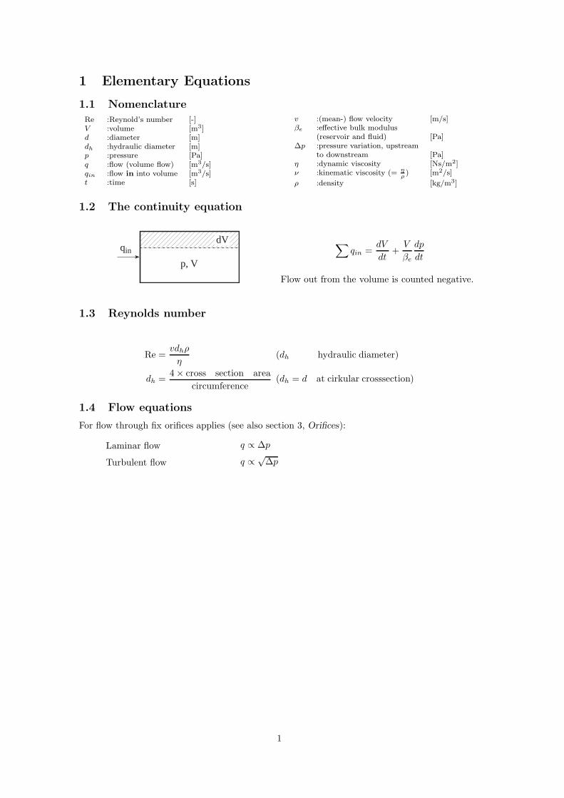
1.2 The continuity equation

p, V

qindV

∑

qin =dV

dt+

V

βe

dp

dt

Flow out from the volume is counted negative.

1.3 Reynolds number

Re =vdhρ

η(dh hydraulic diameter)

dh =4 × cross section area

circumference(dh = d at cirkular crosssection)

1.4 Flow equations

For flow through fix orifices applies (see also section 3, Orifices):

Laminar flow q ∝ ∆p

Turbulent flow q ∝ √∆p

1

2 Pipe flow

2.1 Nomenclature

Re :Reynolds number [-]d :diameter [m]d1 :upstream diameter [m]d2 :downstream diameter [m]h :height [m]h1 :upstream height [m]h2 :downstream height [m]g :gravitation [m/s2]ℓ :length [m]ℓx :distance after disturbance source [m]ℓs :distance after disturbance source

when the flow profile iscompletely developed [m]

p :pressure [Pa]p1 :upstream pressure [Pa]p2 :downstream pressure [Pa]r :radius [m]v :(mean-) flow velocity [m/s]v1 :upstream (mean-) flow velocity [m/s]v2 :downstream (mean-) flow velocity [m/s]α :correction factor [-]∆pf :pressure loss, upstream

to downstream [Pa]ϕ :angle [◦]λ :friction factor [-]ρ :density [kg/m3]ζ :single loss factor [-]ζs :disturbance source factor [-]

2.2 Bernoullis extended equation

At stationary incompressible flow

p1 +ρv2

1

2+ ρgh1 = p2 +

ρv22

2+ ρgh2 + ∆pf

2.3 The flow loss, ∆pf

∆pf =

λℓ

d

ρv2

2at a straight distance

ζs

ρv2

2after a disturbance source

ζρv2

2at a single disturbance source

2.4 The friction factor, λ

λ =

64

ReRe < 2300 laminar flow

0,3164√Re

2300 < Re < 105 turbulent flow in smooth pips

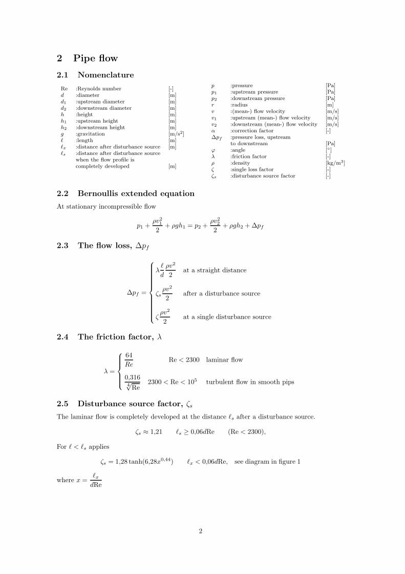
2.5 Disturbance source factor, ζs

The laminar flow is completely developed at the distance ℓs after a disturbance source.

ζs ≈ 1,21 ℓs ≥ 0,06dRe (Re < 2300),

For ℓ < ℓs applies

ζs = 1,28 tanh(6,28x0,44) ℓx < 0,06dRe, see diagram in figure 1

where x =ℓx

dRe

2

1,30

1,00

0,50

0,0010010-110-210-310-410-5

0,06

lx / d Re

ζs

Figur 1: The disturbance source factor ζs as function ofℓx

dRe.

The turbulant flow is completely developed at the distance ℓs after a disturbance source.

ζs ≈ 0,09 ℓs ≥ 40d (Re > 2300),

For ℓ < ℓs applies

ζs = 0,09

√

ℓx

40dℓx < 40d

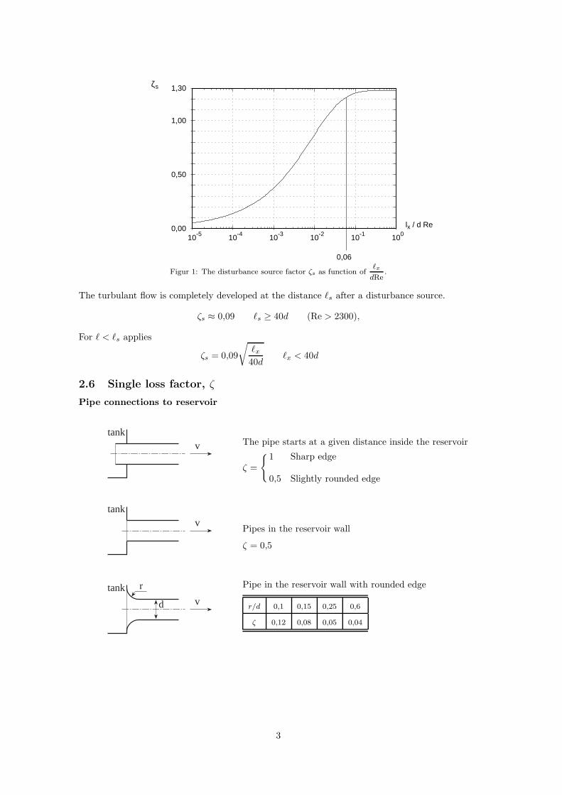
2.6 Single loss factor, ζ

Pipe connections to reservoir

vtank

The pipe starts at a given distance inside the reservoir

ζ =

{

1 Sharp edge

0,5 Slightly rounded edge

vtank

Pipes in the reservoir wall

ζ = 0,5

vtank

d

r Pipe in the reservoir wall with rounded edge

r/d 0,1 0,15 0,25 0,6

ζ 0,12 0,08 0,05 0,04

3

v

tank

dϕ

l

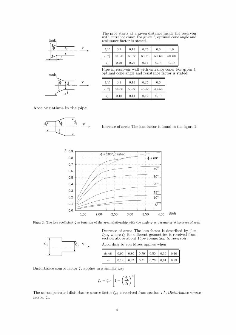
The pipe starts at a given distance inside the reservoirwith entrance cone: For given ℓ, optimal cone angle andresistance factor is stated.

ℓ/d 0,1 0,15 0,25 0,6 1,0

ϕ[◦] 60–90 60–80 60–70 50–60 50–60

ζ 0,40 0,26 0,17 0,13 0,10

v

tank

dϕ

l

Pipe in reservoir wall with entrance cone: For given ℓ,optimal cone angle and resistance factor is stated.

ℓ/d 0,1 0,15 0,25 0,6

ϕ[◦] 50–60 50–60 45–55 40–50

ζ 0,18 0,14 0,12 0,10

Area variations in the pipe

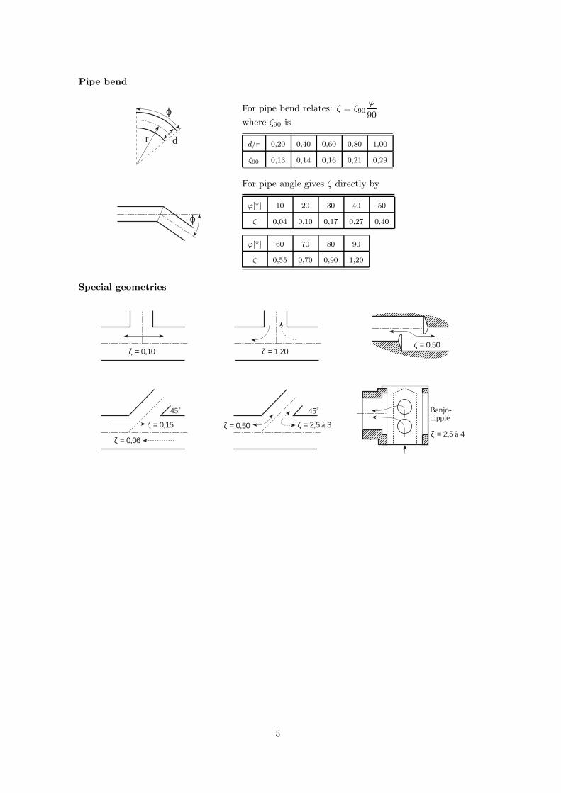
vd2ϕd1 Increase of area: The loss factor is found in the figure 2

0,9

0,8

0,7

0,6

0,5

0,4

0,3

0,2

0,1

0,04,003,503,002,502,001,50

ϕ = 180°, dashedϕ = 60°

40°

30°

20°

15°10°

5°

d2/d1

ζ

Figur 2: The loss coefficient ζ as function of the area relationship with the angle ϕ as parameter at increase of area.

vd2d1

Decrease of area: The loss factor is described by ζ =ζ0α, where ζ0 for different geometries is received fromsection above about Pipe connection to reservoir.

According to von Mises applies when

d2/d1 0,90 0,80 0,70 0,50 0,30 0,10

α 0,19 0,37 0,51 0,76 0,91 0,99

Disturbance source factor ζs applies in a similar way

ζs = ζs0

[

1 −(

d2

d1

)3]

The uncompensated disturbance source factor ζs0 is received from section 2.5, Disturbance source

factor, ζs.

4

Pipe bend

ϕ

r d

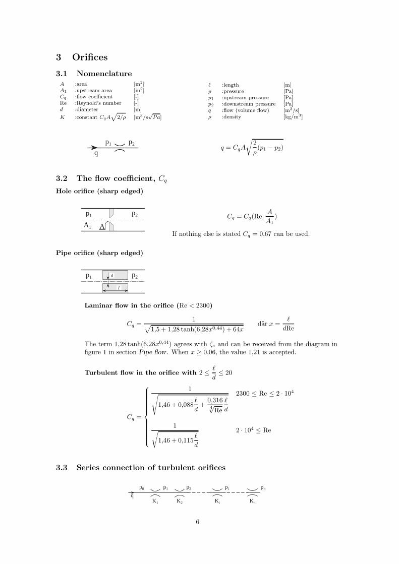
For pipe bend relates: ζ = ζ90ϕ

90where ζ90 is

d/r 0,20 0,40 0,60 0,80 1,00

ζ90 0,13 0,14 0,16 0,21 0,29

ϕ

For pipe angle gives ζ directly by

ϕ[◦] 10 20 30 40 50

ζ 0,04 0,10 0,17 0,27 0,40

ϕ[◦] 60 70 80 90

ζ 0,55 0,70 0,90 1,20

Special geometries

ζ = 0,10 ζ = 1,20ζ = 0,50

ζ = 0,06

ζ = 0,15

45˚

ζ = 0,50 ζ = 2,5 à 3

45˚ Banjo-nipple

ζ = 2,5 à 4

5

3 Orifices

3.1 NomenclatureA :area [m2]A1 :upstream area [m2]Cq :flow coefficient [-]Re :Reynold’s number [-]d :diameter [m]

K :constant CqA√

2/ρ [m3/s√

Pa]

ℓ :length [m]p :pressure [Pa]p1 :upstream pressure [Pa]p2 :downstream pressure [Pa]q :flow (volume flow) [m3/s]ρ :density [kg/m3]

q

p1 p2q = CqA

√

2

ρ(p1 − p2)

3.2 The flow coefficient, Cq

Hole orifice (sharp edged)

p1 p2

A1 A

Cq = Cq(Re,A

A1)

If nothing else is stated Cq = 0,67 can be used.

Pipe orifice (sharp edged)

p1 p2

l

d

Laminar flow in the orifice (Re < 2300)

Cq =1

√

1,5 + 1,28 tanh(6,28x0,44) + 64xdar x =

ℓ

dRe

The term 1,28 tanh(6,28x0,44) agrees with ζs and can be received from the diagram infigure 1 in section Pipe flow . When x ≥ 0,06, the value 1,21 is accepted.

Turbulent flow in the orifice with 2 ≤ ℓ

d≤ 20

Cq =

1√

1,46 + 0,088ℓ

d+

0,3164√Re

ℓ

d

2300 ≤ Re ≤ 2 · 104

1√

1,46 + 0,115ℓ

d

2 · 104 ≤ Re

3.3 Series connection of turbulent orifices

p1 p2

KnK iK2K1

q

p0 pi pn

6

The sum of the orifices applies:

q = K√

p0 − pn dar K =1

√

√

√

√

n∑

i=1

1

K2i

Ki = CqiAi

√

2

ρ

The pressure after the j:th orifice is given by

pj = p0 − (p0 − pn)K2

j∑

i=1

1

K2i

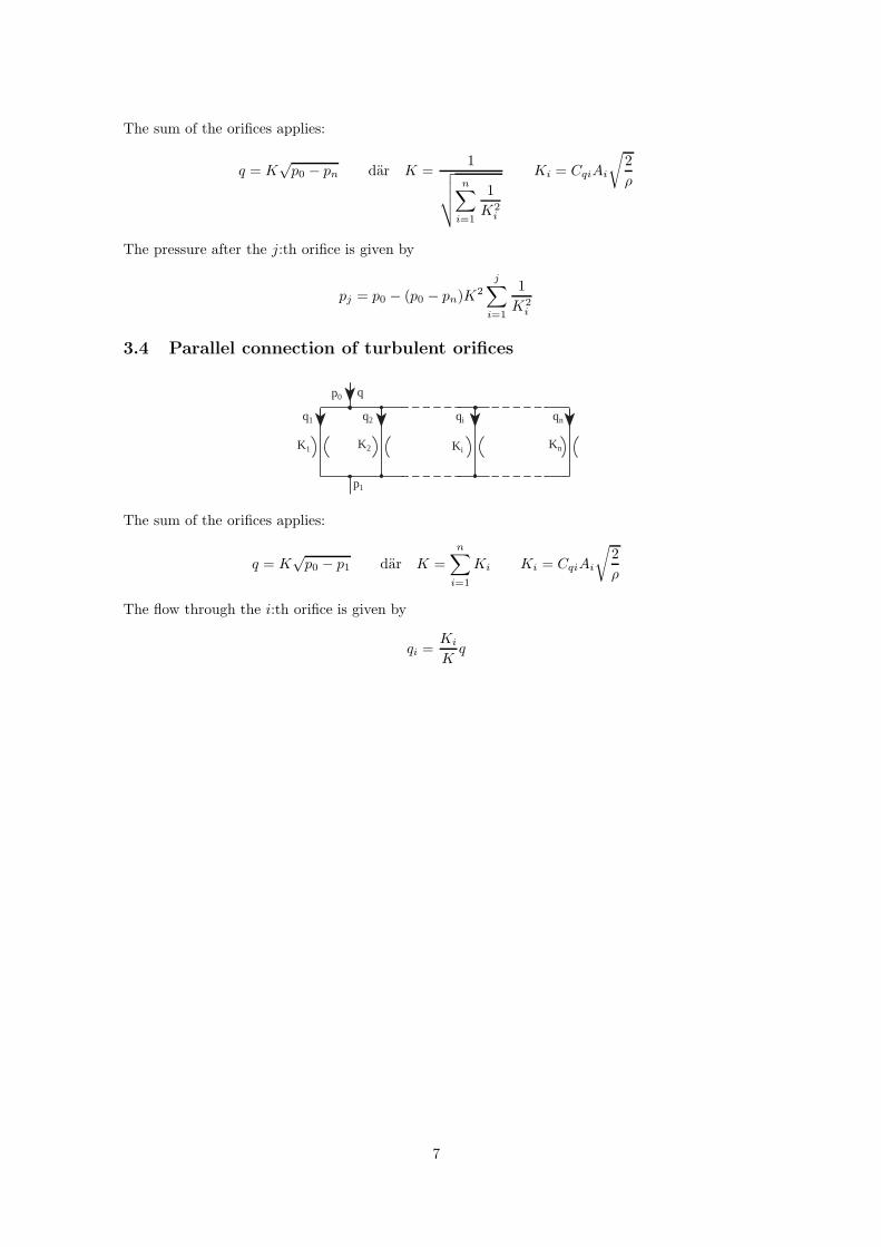
3.4 Parallel connection of turbulent orifices

p1

p0

KnK iK2K1

q

q1 q2 qi qn

The sum of the orifices applies:

q = K√

p0 − p1 dar K =n

∑

i=1

Ki Ki = CqiAi

√

2

ρ

The flow through the i:th orifice is given by

qi =Ki

Kq

7

4 Flow forces

4.1 NomenclatureFs :flow force [N]d :spool diameter [m]ℓ :length [m]p :pressure [Pa]p1 :upstream pressure [Pa]p2 :downstream pressure [Pa]

q :flow (volume flow) [m3/s]v :(mean-)flow velocity [m/s]w :area gradient [m]x :spool opening [m]δ :jet angle [◦]ρ :density [kg/m3]

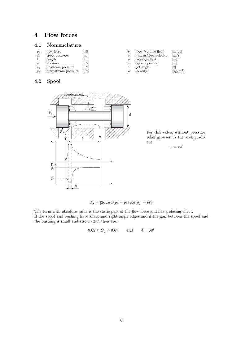
4.2 Spool

Fluidelement

Fs d

v

pp1

p2

l

δ

x

For this valve, without pressurerelief grooves, is the area gradi-ent:

w = πd

Fs = |2Cqwx(p1 − p2) cos(δ)| + ρℓq

The term with absolute value is the static part of the flow force and has a closing effect.If the spool and bushing have sharp and right angle edges and if the gap between the spool andthe bushing is small and also x ≪ d, then are:

0,62 ≤ Cq ≤ 0,67 and δ = 69◦

8

5 Rotational transmissions

5.1 NomenclatureCv :laminar leakage losses [-]D :displacement [m3/rev]Min :driving torque pump [Nm]Mut :output torque motor [Nm]kp :Coulomb friction [-]kv :viscous friction losses [-]kε :displacement coefficient [-]n :revs [rev/s]

qe :effective flow [m3/s]∆p :pressure difference [Pa]ε :displacement setting [-]ηhm :hydraulic mechanical efficiency [-]ηvol :volumetric efficiency [-]Sub index

p pumpm motor

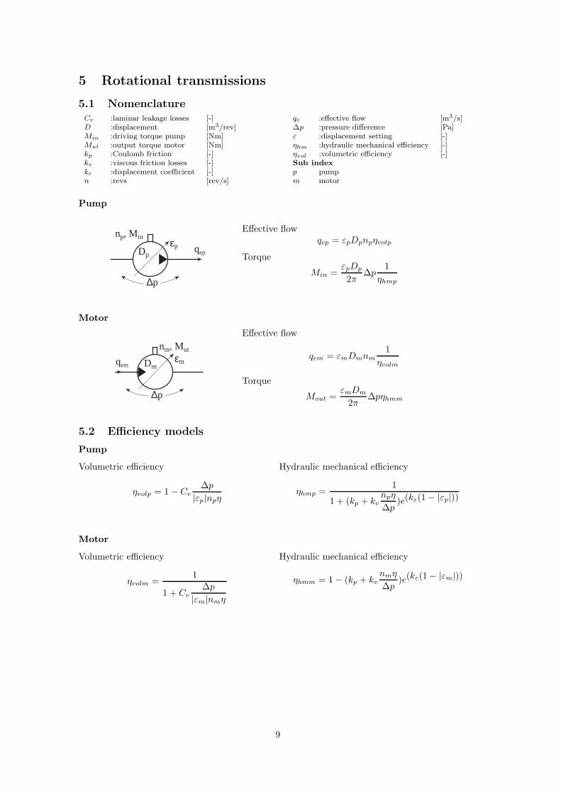
Pump

qep

∆p

np, Minεp

Dp

Effective flowqep = εpDpnpηvolp

Torque

Min =εpDp

2π∆p

1

ηhmp

Motor

qem

∆p

nm, Mut

εmDm

Effective flow

qem = εmDmnm

1

ηvolm

Torque

Mout =εmDm

2π∆pηhmm

5.2 Efficiency models

Pump

Volumetric efficiency

ηvolp = 1 − Cv

∆p

|εp|npη

Hydraulic mechanical efficiency

ηhmp =1

1 + (kp + kv

npη

∆p)e(kε(1 − |εp|))

Motor

Volumetric efficiency

ηvolm =1

1 + Cv

∆p

|εm|nmη

Hydraulic mechanical efficiency

ηhmm = 1 − (kp + kv

nmη

∆p)e(kε(1 − |εm|))

9

6 Accumulators

6.1 NomenclatureV0 :accumulator volume [m3]n :polytrophic exponent [-]p0 :pre-charged pressure (absolute pressure,

normally ≈ 90 % av p1) [Pa]

p1 :minimum working pressure (absolute) [Pa]p2 :maximum working pressure (absolute) [Pa]∆V :working volume [m3]

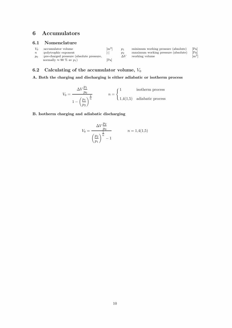
6.2 Calculating of the accumulator volume, V0

A. Both the charging and discharging is either adiabatic or isotherm process

V0 =

∆Vp1

p0

1 −(

p1

p2

)

1n

n =

{

1 isotherm process

1,4(1,5) adiabatic process

B. Isotherm charging and adiabatic discharging

V0 =

∆Vp2

p0

(

p2

p1

)

1n

− 1

n = 1,4(1,5)

10

7 Gap theory

7.1 Nomenclature

Ff :friction force [N]Mf :friction torque [Nm]Pf :power loss [W]b :gap width perpendicular

to flow direction [m]e :eccentricity [m]h :gap height [m]

h0 mean gap height (h1 + h2

2) [m]

ℓ :length [m]

p :pressure [Pa]qℓ :leakage flow [m3/s]r :radius [m]r1 :inner radius [m]r2 :outer radius [m]v :relative velocity [m/s]∆p :pressure difference through

the gap (p1 − p0) [Pa]γ :angle [rad]η :dynamic viscosity [Ns/m2]ω :angular speed [rad/s]

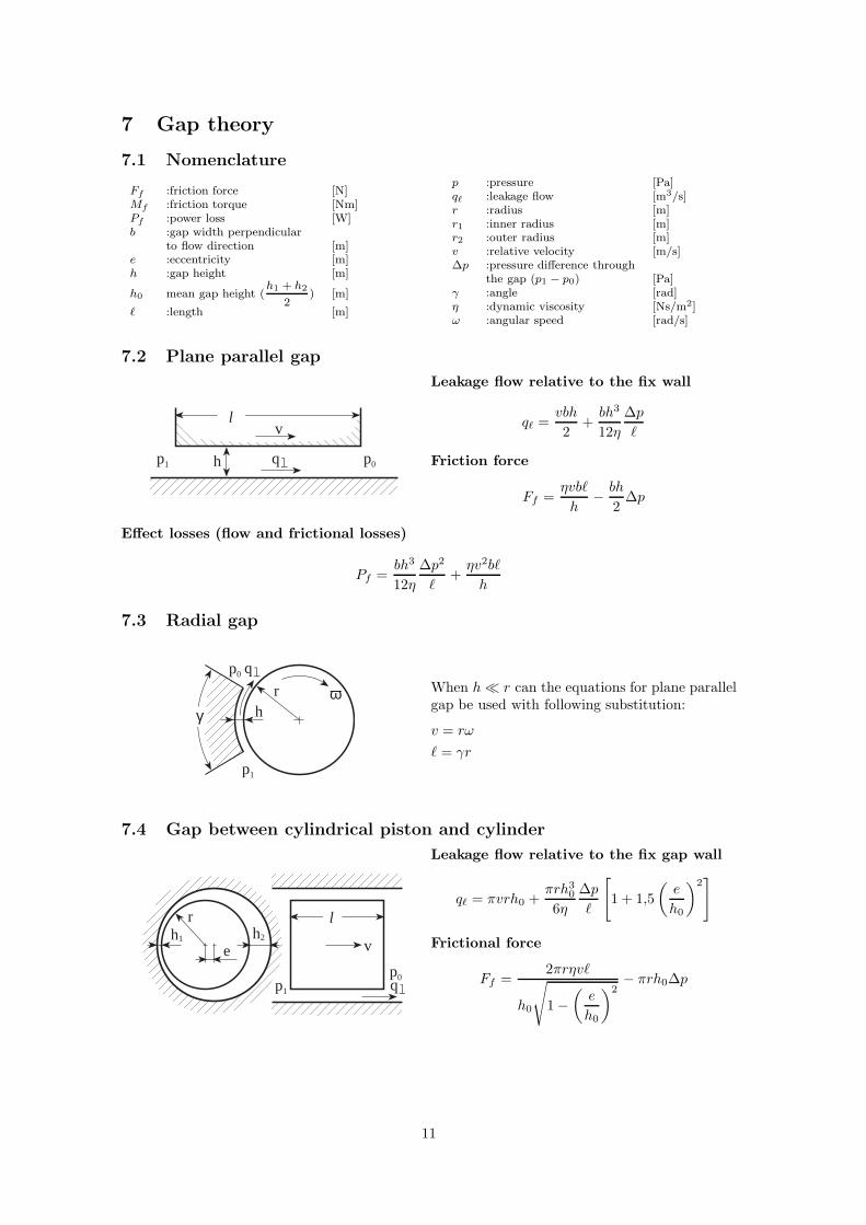
7.2 Plane parallel gap

p1 p0h

vl

ql

Leakage flow relative to the fix wall

qℓ =vbh

2+

bh3

12η

∆p

ℓ

Friction force

Ff =ηvbℓ

h− bh

2∆p

Effect losses (flow and frictional losses)

Pf =bh3

12η

∆p2

ℓ+

ηv2bℓ

h

7.3 Radial gap

p1

p0

hωr

γ

qlWhen h ≪ r can the equations for plane parallelgap be used with following substitution:

v = rω

ℓ = γr

7.4 Gap between cylindrical piston and cylinder

h1

r

e v

l

p0p1

h2

ql

Leakage flow relative to the fix gap wall

qℓ = πvrh0 +πrh3

0

6η

∆p

ℓ

[

1 + 1,5

(

e

h0

)2]

Frictional force

Ff =2πrηvℓ

h0

√

1 −(

e

h0

)2− πrh0∆p

11

Effect losses (flow and frictional losses)

Pf =πrh3

0

6η

∆p2

ℓ

[

1 + 1,5

(

e

h0

)2]

+2πrηv2ℓ

h0

√

1 −(

e

h0

)2

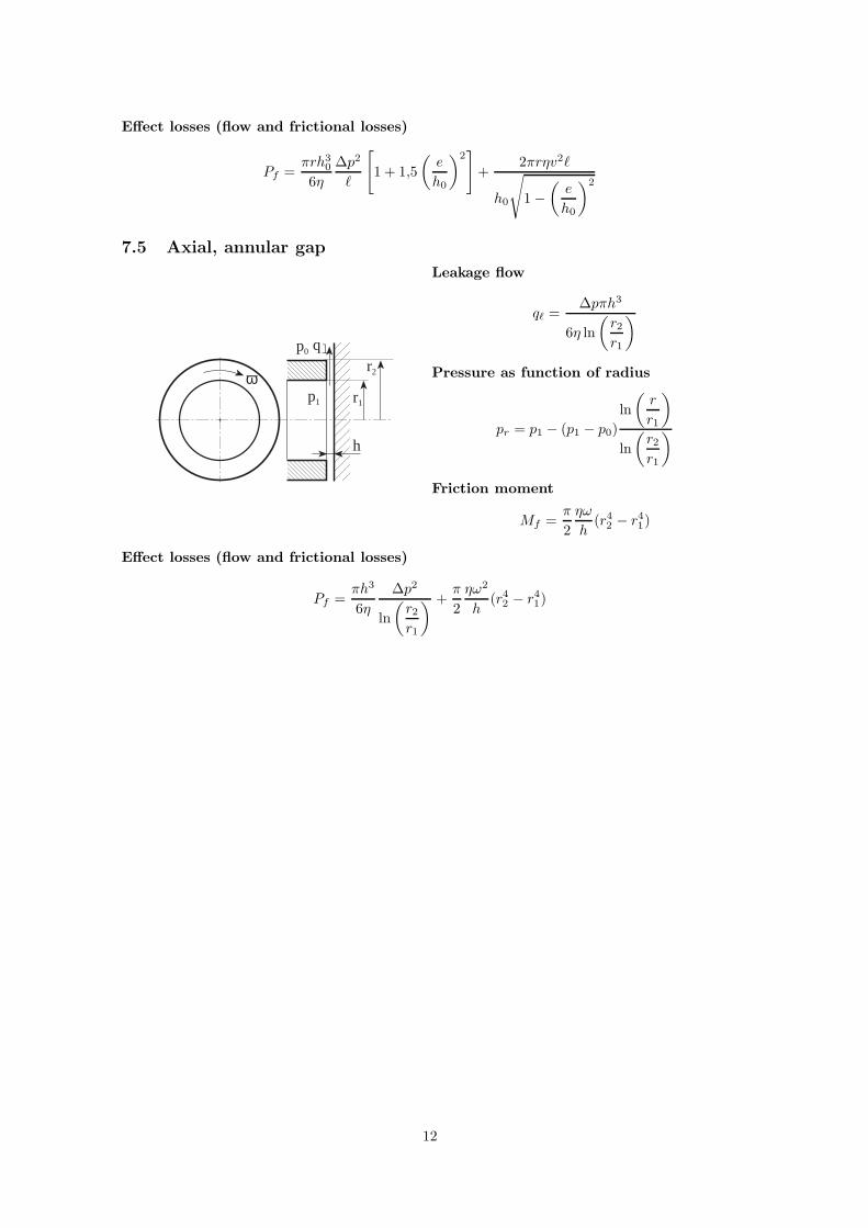
7.5 Axial, annular gap

p0

ωp1

h

r2

r1

ql

Leakage flow

qℓ =∆pπh3

6η ln

(

r2

r1

)

Pressure as function of radius

pr = p1 − (p1 − p0)

ln

(

r

r1

)

ln

(

r2

r1

)

Friction moment

Mf =π

2

ηω

h(r4

2 − r41)

Effect losses (flow and frictional losses)

Pf =πh3

6η

∆p2

ln

(

r2

r1

) +π

2

ηω2

h(r4

2 − r41)

12

8 Hydrostatic bearings

8.1 NomenclatureAe :effective area [m2]B :bearing chamber length [m]F :load [N]K1 :constant [Ns]K2 :constant [Nm2s]L :bearing surface length [m]ae :effective area/width [m]f :load/width [N/m]h :gap height [m]ℓ :length [m]

kb :constant [Ns/m2]k2 :constant [Nms]p :pressure [Pa]pb :pressure in the bearing chamber [Pa]qs :flow through the bearing [m3/s]qsB :flow through

the bearing/width [m2/s]r1 :inner radius [m]r2 :outer radius [m]η :dynamic viscosity [Ns/m2]

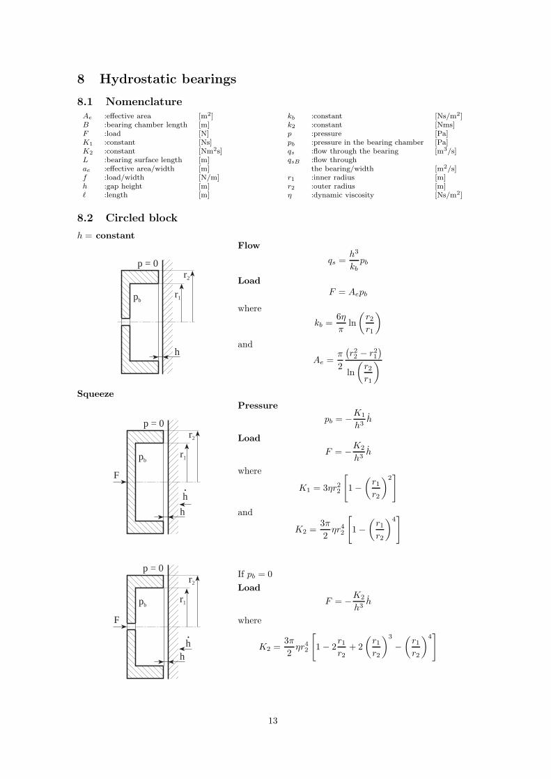
8.2 Circled block

h = constant

pb

h

r2

r1

p = 0

Flow

qs =h3

kb

pb

LoadF = Aepb

where

kb =6η

πln

(

r2

r1

)

and

Ae =π

2

(

r22 − r2

1

)

ln

(

r2

r1

)

Squeeze

pb

h

r2

r1

p = 0

F

h.

Pressure

pb = −K1

h3h

Load

F = −K2

h3h

where

K1 = 3ηr22

[

1 −(

r1

r2

)2]

and

K2 =3π

2ηr4

2

[

1 −(

r1

r2

)4]

pb

h

r2

r1

p = 0

F

h.

If pb = 0

Load

F = −K2

h3h

where

K2 =3π

2ηr4

2

[

1 − 2r1

r2+ 2

(

r1

r2

)3

−(

r1

r2

)4]

13

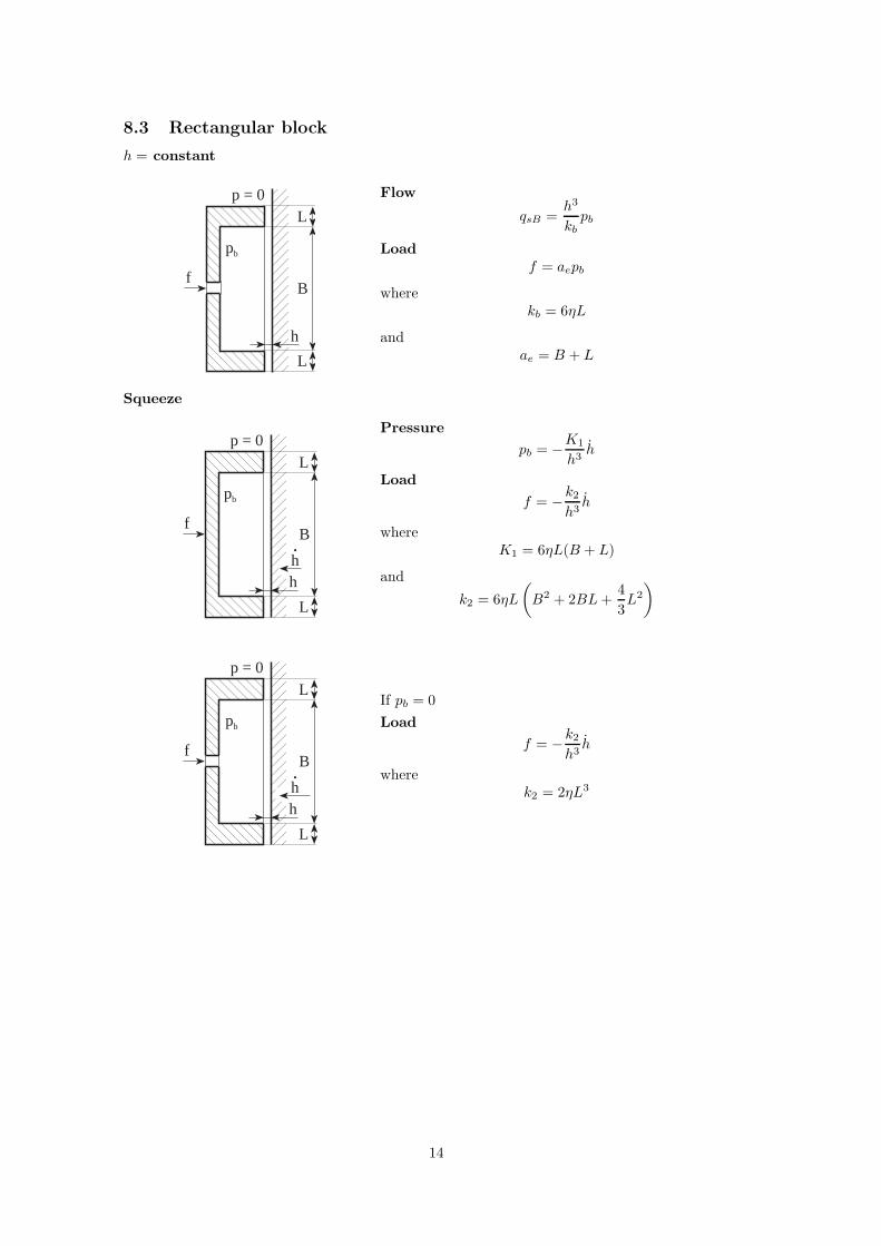
8.3 Rectangular block

h = constant

pb

h

Lp = 0

f

L

B

Flow

qsB =h3

kb

pb

Loadf = aepb

wherekb = 6ηL

andae = B + L

Squeeze

pb

h

Lp = 0

f

L

B

h.

Pressure

pb = −K1

h3h

Load

f = −k2

h3h

whereK1 = 6ηL(B + L)

and

k2 = 6ηL

(

B2 + 2BL +4

3L2

)

pb

h

Lp = 0

f

L

B

h.

If pb = 0

Load

f = −k2

h3h

wherek2 = 2ηL3

14

9 Hydrodynamic bearing theory

9.1 Nomenclature

U1 :velocity in x-axis surface 1 [m/s]U2 :velocity in x-axis surface 2 [m/s]V1 :velocity in y-axis surface 1 [m/s]V2 :velocity in y-axis surface 2 [m/s]T :temperature [K]c :specific heat [kJ/kg K]h :gap height [m]p :pressure [Pa]qx :flow/width unit in x-axis [m2/s]qz :flow/width unit in z-axis [m2/s]qr :flow/width unit in r-axis [m2/s]

qθ :flow/width unit in θ-axis [m2/s]r :radius [m]t :time [s]u :flow velocity in x-axis [m/s]w :flow velocity in z-axis [m/s]η :dynamic viscosity [Ns/m2]τx :shear stress in x-axis [N/m2]τθ :shear stress in θ-axis [N/m2]ρ :density [kg/m3]ω1 :velocity in θ-axis surface 1 [rad/s]ω2 :velocity in θ-axis surface 2 [rad/s]θ :angle [rad]

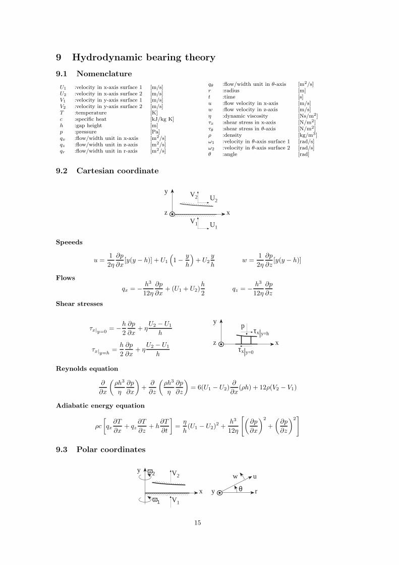
9.2 Cartesian coordinate

V1 U1

V2 U2

x

y

z

Speeeds

u =1

2η

∂p

∂x[y(y − h)] + U1

(

1 − y

h

)

+ U2y

hw =

1

2η

∂p

∂z[y(y − h)]

Flows

qx = − h3

12η

∂p

∂x+ (U1 + U2)

h

2qz = − h3

12η

∂p

∂z

Shear stresses

τx|y=0= −h

2

∂p

∂x+ η

U2 − U1

h

τx|y=h=

h

2

∂p

∂x+ η

U2 − U1

h

p

x

y

z

τx|y=h

τx|y=0

Reynolds equation

∂

∂x

(

ρh3

η

∂p

∂x

)

+∂

∂z

(

ρh3

η

∂p

∂z

)

= 6(U1 − U2)∂

∂x(ρh) + 12ρ(V2 − V1)

Adiabatic energy equation

ρc

[

qx

∂T

∂x+ qz

∂T

∂z+ h

∂T

∂t

]

=η

h(U1 − U2)

2 +h3

12η

[

(

∂p

∂x

)2

+

(

∂p

∂z

)2]

9.3 Polar coordinates

rθ

w

y

u

V1ω1

V2ω2

x

y

15

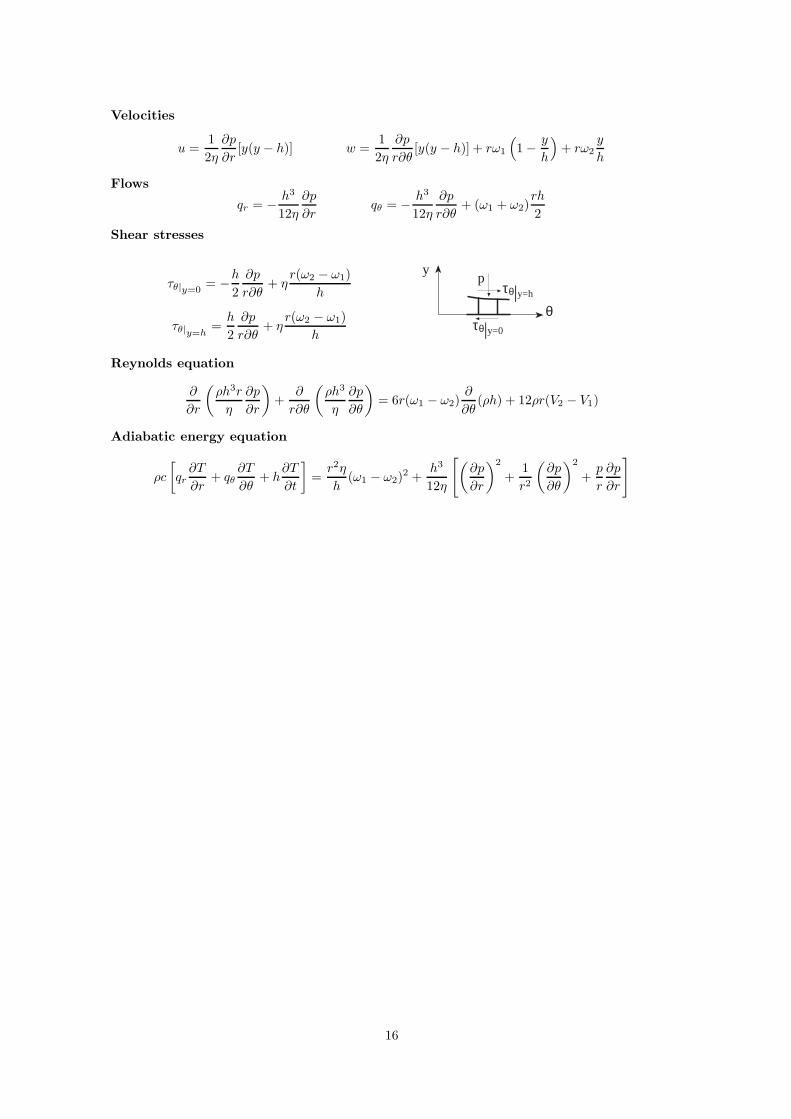
Velocities

u =1

2η

∂p

∂r[y(y − h)] w =

1

2η

∂p

r∂θ[y(y − h)] + rω1

(

1 − y

h

)

+ rω2y

h

Flows

qr = − h3

12η

∂p

∂rqθ = − h3

12η

∂p

r∂θ+ (ω1 + ω2)

rh

2

Shear stresses

τθ|y=0= −h

2

∂p

r∂θ+ η

r(ω2 − ω1)

h

τθ|y=h=

h

2

∂p

r∂θ+ η

r(ω2 − ω1)

h

p

θ

yτθ|y=h

τθ|y=0

Reynolds equation

∂

∂r

(

ρh3r

η

∂p

∂r

)

+∂

r∂θ

(

ρh3

η

∂p

∂θ

)

= 6r(ω1 − ω2)∂

∂θ(ρh) + 12ρr(V2 − V1)

Adiabatic energy equation

ρc

[

qr

∂T

∂r+ qθ

∂T

∂θ+ h

∂T

∂t

]

=r2η

h(ω1 − ω2)

2 +h3

12η

[

(

∂p

∂r

)2

+1

r2

(

∂p

∂θ

)2

+p

r

∂p

∂r

]

16

10 Non-stationary flow

10.1 Nomenclature

A :line sectional area [m2]B :constant (L0a) [kg/s m4]CH :conc. hydr. capacitance [m5/N]C0 :conc. hydr. capacitance/l.enh. [m4/N]F :force [N]LH :conc. hydr. inductance [kg/m4]L0 :conc. hydr. inductance/l.enh. [kg/m5]P :pressure (frequency dependent) [Pa]Q :flow (volume flow) (frequency dependent) [m3/s]RHℓ :conc. hydr. resistance (lam.) [Ns/m5]RHt :conc. hydr. resistance (turb.) [Ns/m5]R0ℓ :conc. hydr. res./l.unit. (lam.) [Ns/m6]R0t :conc. hydr. res./l.unit. (turb.) [Ns/m6]V1 :volume [m3]V2 :volume [m3]Z0 :impedance [Ns/m5]a :speed of sound [m/s]d :diameter [m]ℓ :length [m]m :mass [kg]

p :pressure [Pa]p0 :pressure in point of operation [Pa]p1 :upstream pressure [Pa]p2 :downstream pressure [Pa]ps :supply pressure [Pa]q :flow (volume flow) [m3/s]q0 :flow in point of operation [m3/s]s :Laplace operator (iω) [1/s]t :time [s]tv :valve closing time [s]v0 :flow velocity [m/s]

:velocity of cylinder [m/s]α :dimensionless area [-]βe :effective bulk modulus [Pa]∆p :change in pressure due to pressure peek [Pa]η :dynamic viscosity [Ns/m2]λ :friction coefficient [-]

:parameter [1/m]ρ :density [kg/m3]ζ :single resistant loss [-]

10.2 Joukowskis equation

∆p = ρav0

Reduction due to valve closing time.

∆pred = ∆p2ℓ

atvfor tv >

2ℓ

a

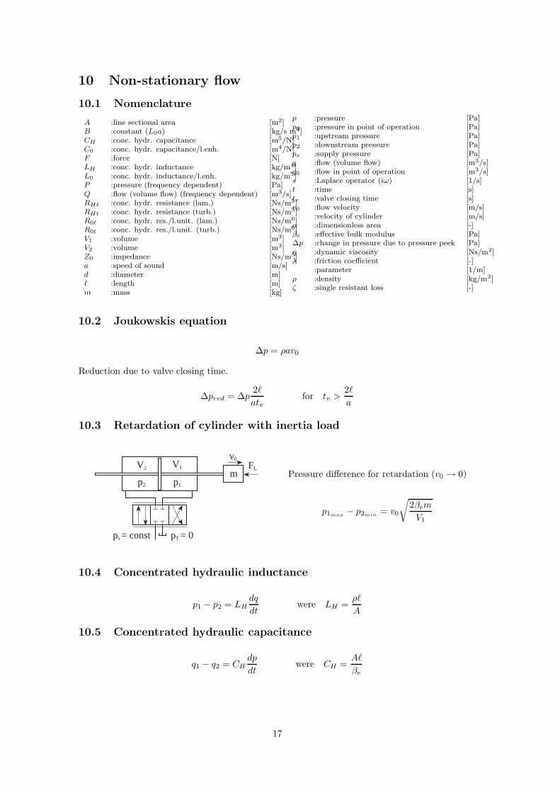
10.3 Retardation of cylinder with inertia load

mFLV1

p1

V2

p2

pT = 0ps = const

v0

Pressure difference for retardation (v0 → 0)

p1max− p2min

= v0

√

2βem

V1

10.4 Concentrated hydraulic inductance

p1 − p2 = LH

dq

dtwere LH =

ρℓ

A

10.5 Concentrated hydraulic capacitance

q1 − q2 = CH

dp

dtwere CH =

Aℓ

βe

17

10.6 Concentrated hydraulic resistance

p1−p2 = RHq were RH =

RHℓ =128ηℓ

πd4For laminar flow

RHt = λℓ

d

ρq0

A2

For turbulent flow,with linearization around the workingpoint with the flow q0

10.7 Basic differential equations on flow systems with parameter dis-tribution in space

∂p

∂x+ L0

∂q

∂t+ R0q|q|m = 0

∂q

∂x+ C0

∂p

∂t= 0

Parameter values (per length unit)independent of flow regime

C0 =A

βe

L0 =ρ

A

with laminar flow

R0ℓ =128η

πd4m = 0

with turbulent flow

R0t =0,1582 η0,25 ρ0,75

d1,25 A1,75m = 0,75

10.8 Speed of waves in pipes filled with liquid

a =1√

L0C0

=

√

βe

ρ

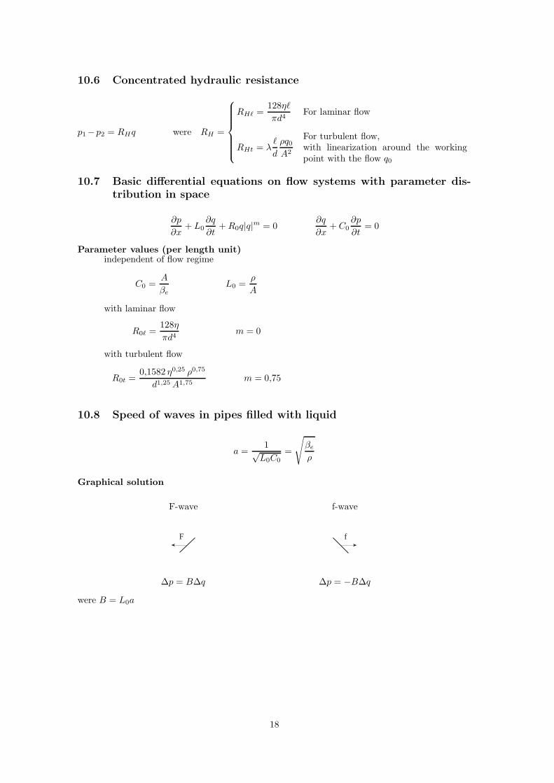
Graphical solution

F-wave

F

∆p = B∆q

f-wave

f

∆p = −B∆q

were B = L0a

18

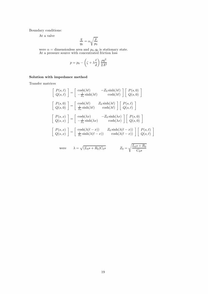
Boundary conditions:

At a valveq

q0= α

√

p

p0

were α = dimensionless area and p0, q0 is stationary state.At a pressure source with concentrated friction loss

p = p0 −(

ζ + λℓ

d

)

ρq2

2A2

Solution with impedance method

Transfer matrices[

P (s, ℓ)Q(s, ℓ)

]

=

[

cosh(λℓ) −Z0 sinh(λℓ)− 1

Z0sinh(λℓ) cosh(λℓ)

] [

P (s, 0)Q(s, 0)

]

[

P (s, 0)Q(s, 0)

]

=

[

cosh(λℓ) Z0 sinh(λℓ)1

Z0sinh(λℓ) cosh(λℓ)

] [

P (s, ℓ)Q(s, ℓ)

]

[

P (s, x)Q(s, x)

]

=

[

cosh(λx) −Z0 sinh(λx)− 1

Z0sinh(λx) cosh(λx)

] [

P (s, 0)Q(s, 0)

]

[

P (s, x)Q(s, x)

]

=

[

cosh(λ(ℓ − x)) Z0 sinh(λ(ℓ − x))1

Z0sinh(λ(ℓ − x)) cosh(λ(ℓ − x))

] [

P (s, ℓ)Q(s, ℓ)

]

were λ =√

(L0s + R0)C0s Z0 =

√

L0s + R0

C0s

19

11 Pump pulsations

11.1 NomenclatureA :the pipe’s cross-sectional area [m2]T :wave propagation time [s]D :pump displacement [m3/varv]L :pipe length [m]P :pulsation amplitude [N/m2]V :volume [m3]a :wave propagation speed [m/s]d :pipe diameter [m]fp :dim. free flow spectrum [-]n :pump speed [rev/s]

ps :static pressure level [Pa]z :the pump’s piston number [-]η :dynamic viscosity [Ns/m2]αp :dim.free cylinder volume [-]β :bulk modulus [Pa]ε :the pump’s displacement [-]γ :dim.free dead volume [-]ρ :density [kg/m3]τ :dim.free charging time [-]ω :angular frequency [rad/s]

11.2 System with closed end

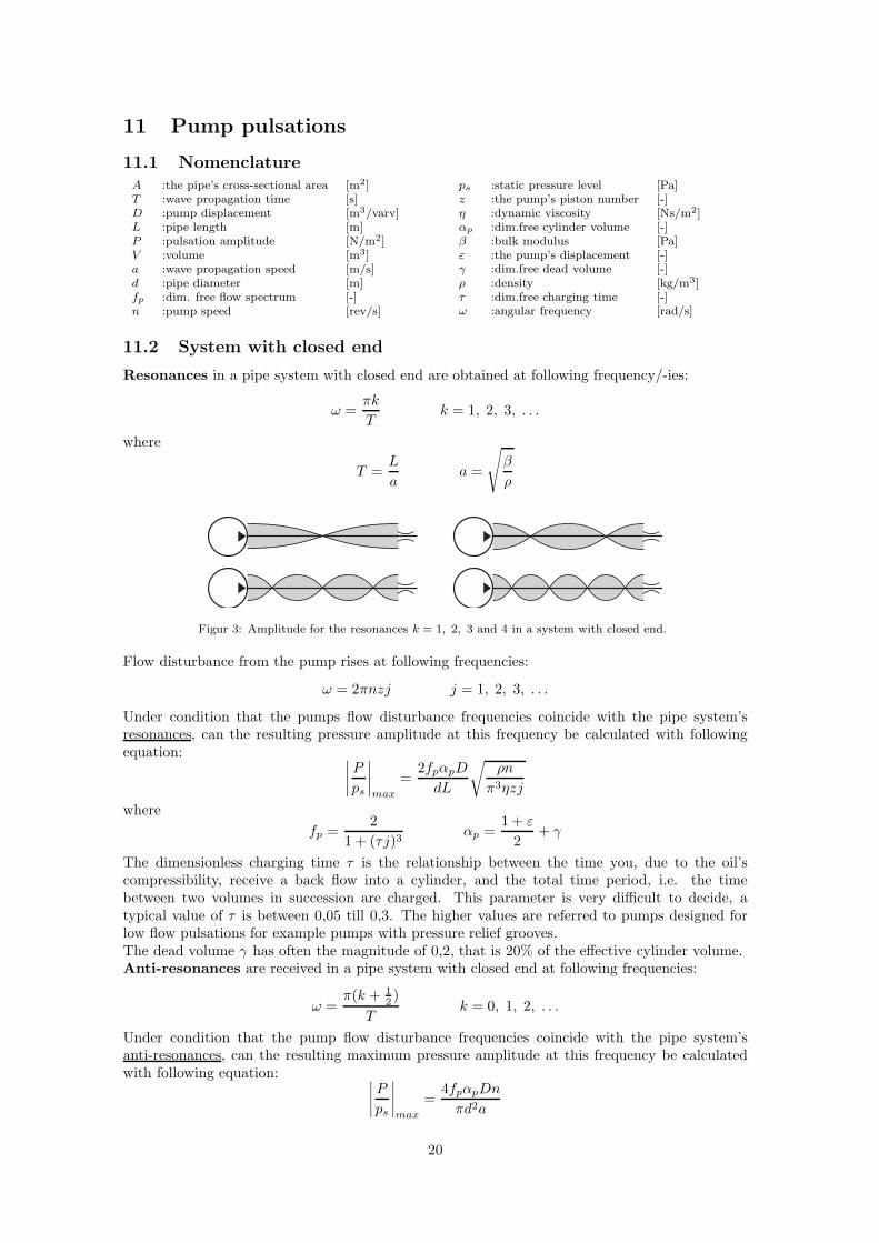
Resonances in a pipe system with closed end are obtained at following frequency/-ies:

ω =πk

Tk = 1, 2, 3, . . .

where

T =L

aa =

√

β

ρ

Figur 3: Amplitude for the resonances k = 1, 2, 3 and 4 in a system with closed end.

Flow disturbance from the pump rises at following frequencies:

ω = 2πnzj j = 1, 2, 3, . . .

Under condition that the pumps flow disturbance frequencies coincide with the pipe system’sresonances, can the resulting pressure amplitude at this frequency be calculated with followingequation:

∣

∣

∣

∣

P

ps

∣

∣

∣

∣

max

=2fpαpD

dL

√

ρn

π3ηzj

where

fp =2

1 + (τj)3αp =

1 + ε

2+ γ

The dimensionless charging time τ is the relationship between the time you, due to the oil’scompressibility, receive a back flow into a cylinder, and the total time period, i.e. the timebetween two volumes in succession are charged. This parameter is very difficult to decide, atypical value of τ is between 0,05 till 0,3. The higher values are referred to pumps designed forlow flow pulsations for example pumps with pressure relief grooves.The dead volume γ has often the magnitude of 0,2, that is 20% of the effective cylinder volume.Anti-resonances are received in a pipe system with closed end at following frequencies:

ω =π(k + 1

2 )

Tk = 0, 1, 2, . . .

Under condition that the pump flow disturbance frequencies coincide with the pipe system’santi-resonances, can the resulting maximum pressure amplitude at this frequency be calculatedwith following equation:

∣

∣

∣

∣

P

ps

∣

∣

∣

∣

max

=4fpαpDn

πd2a

20

Example: The above equations are used for following example. A constant pressure pumppresumed work against a closed valve. Following data is obtained:

d = 38 · 10−3 [m]n = 25 [rev/s]z = 9D = 220 · 10−6 [m3/rev]βe = 1,5 · 109 [Pa]

γ = 0,2ε = 0η = 0,02 [Ns/m2]ρ = 900 [kg/m3]τ = 0,25

Four different pipe lengths between pump and valve is analysed:

L = 1,45 m Gives resonances for j = 2, 4, 6, . . . anti-resonances for j = 1, 3, 5, . . .L = 1,91 m Gives resonance for j = 3, 6, . . . no anti-resonanceL = 2,15 m Gives resonance for j = 4, . . . anti-resonances for j = 2, 6, . . .L = 2,90 m Gives resonance for j = 1, 2, 3, . . . no anti-resonance

In the table below shows the obtained relationship between pulsation’s pressure amplitude and thesystem’s pressure level for respective disturbance harmonic. Note, for L = 1,91 m and L = 2,15 mcan some disturbance harmonics not be analysed with the equations above, since they don’tcoincide with any of the pipe’s resonances or anti-resonances. However, the amplitudes at thesefrequencies are relative small because they don’t coincide with any of the pipe’s resonances. Inthe table below, these values are in parenthesis.

Relative pulsation amplitude |P/ps|

j f [Hz] L = 1,45 m L = 1,91 m L = 2,15 m L = 2,90 m

1 225 0,01 (0,01) (0,01) 0,35

2 450 0,45 (0,01) 0,00 0,22

3 675 0,00 0,22 (0,01) 0,14

4 900 0,18 (0,00) 0,12 0,09

5 1125 0,00 (0,00) (0,01) 0,05

6 1350 0,07 0,05 0,00 0,03

11.3 Systems with low end impedance (e.g. volume)

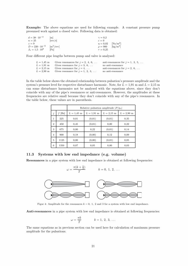
Resonances in a pipe system with low end impedance is obtained at following frequencies:

ω =π(k + 1

2 )

Tk = 0, 1, 2, . . .

Figur 4: Amplitude for the resonances k = 0, 1, 2 and 3 for a system with low end impedance.

Anti-resonances in a pipe system with low end impedance is obtained at following frequencies:

ω =πk

Tk = 1, 2, 3, . . .

The same equations as in previous section can be used here for calculation of maximum pressureamplitude for the pulsations.

21

If a volume, which size is not infinite, is connected to the pipe system is a dislocation of theline’s resonances from the values in above equations obtained. This dislocation can be calculatedaccording to following equation

∆ω =1

T

[

π

2− arctan

(

V ω

Aa

)]

I.e. if a finite volume is used the resonance frequency is increased.As example on this section, a high pressure filter is placed before the valve in the example withthe constant pressure pump. The valve is closed in this example too. The volume of the filter is2 liters; other parameters are the same as the previous example except for the length of the line.The following line lengths are analysed:

L = 1,47 m Gives resonance for j = 3, 5, . . . anti-resonance for j = 2, 4, 6, . . .L = 1,87 m Gives resonance for j = 1, 4, . . . anti-resonance for j = 3, 6, . . .L = 3,00 m Gives no resonance anti-resonance for j = 1, 2, 3, 4, 5, 6, . . .

Note, the volume is relative small and therefore the dislocation equation has to be used. Whenthe new resonance frequency is calculated, ”‘passningsrakning”’ has to be used. The method isshown bellow for L = 1,47 m and k = 1.

ω =π

(

k + 12

)

T= 1350rad/s ⇒

∆ω = 430 rad/s ω = 1810 rad/s∆ω = 340 rad/s ω = 1720 rad/s∆ω = 350 rad/s ω = 1730 rad/s

The size of the pulsation amplitude in relation to the static system pressure is shown in the tablebelow. The values in parenthesis show, as in previous example, a more correct analyze of thedisturbance harmonic which can not be calculated with the equation given in this handbook.

Relative pulsation amplitude |P/ps|

j f [Hz] L = 1,47 m L = 1,87 m L = 3,00 m

1 225 (0,01) (0,54) 0,01

2 450 0,00 (0,01) 0,00

3 675 0,28 0,00 0,00

4 900 0,00 0,14 0,00

5 1125 0,11 (0,00) 0,00

6 1350 0,00 0,00 0,00

22

12 Hydraulic servo systems

12.1 Nomenclature

A :piston area [m2]Ah :control piston area (3-port valve) [m2]Am :amplitude margin [dB]Ar :piston area, rod side

(3-port valve) [m2]Au :the open system’s transfer functionBm :viscous friction coeff. (motor) [Nms/rad]Bp :viscous friction coeff. (cylinder) [Ns/m]Ce :external leakage flow coeff.

(cylinder/motor/pump) [m5/Ns]Ci :internal leakage flow coeff.

(cylinder/motor/pump) [m5/Ns]Ct :total leakage flow coeff. [m5/Ns]Cq :leakage flow coeff. [-]D :displacement (motor/pump) [m3/rad]FL :external (load-) force on cylinder [N]Gc :the closed system’s transfer functionGo :the open system’s transfer functionGreg :controller transfer functionJt :total moment of inertia

(motor and load) [kg m2]Kc :flowpressure coeff. (servo valve) [m5/Ns]Kp :pressure gain (servo valve) [Pa/m]Kq :flow gain (servo valve) [m2/s]Kreg :control gainKv :loop gainMt :total mass (cylinder piston

and load) [kg]Np :pump speed [rad/s]S :stiffnessTL :external (load-)moment on motor [Nm]U :under lap [m]V :volume [m3]

Vh :control volume (3-port valve) [m3]Vt :total volume [m3]e :control errorkp :displacement gradient (pump) [m3/rad2]p :pressure [Pa]pc :control pressure (3-port valve) [Pa]ps :supply pressure [Pa]q :flow (volume flow) [m3/s]qc :centre flow [m3/s]s :Laplace operator (iω) [rad/s]t :time [s]xv :position (servo valve) [m]xp :position (cylinder piston) [m]w :area gradient [m]βe :effective bulk modulus [Pa]δh :hydraulic damping [-]ε0 :control error (stationary)ρ :density [kg/m3]θm :angular position (motor) [rad]φp :displacement angle (pump) [rad]ϕm :phase margin [◦]ω :angular frequency [rad/s]ωb :bandwidth [rad/s]ωc :crossing-out frequency [rad/s]ωh :hydraulic eigen frequency [rad/s]Re :real partIm :imaginary part

Tillaggsindex0 :working pointe :effectivem :motorp :cylinder (piston), pumpv :valvet :totalL :load

23

12.2 Introduction

The servo technical section discusses following system:

• valve controlled cylinder

• valve controlled motor

• pump controlled cylinder

• pump controlled motor

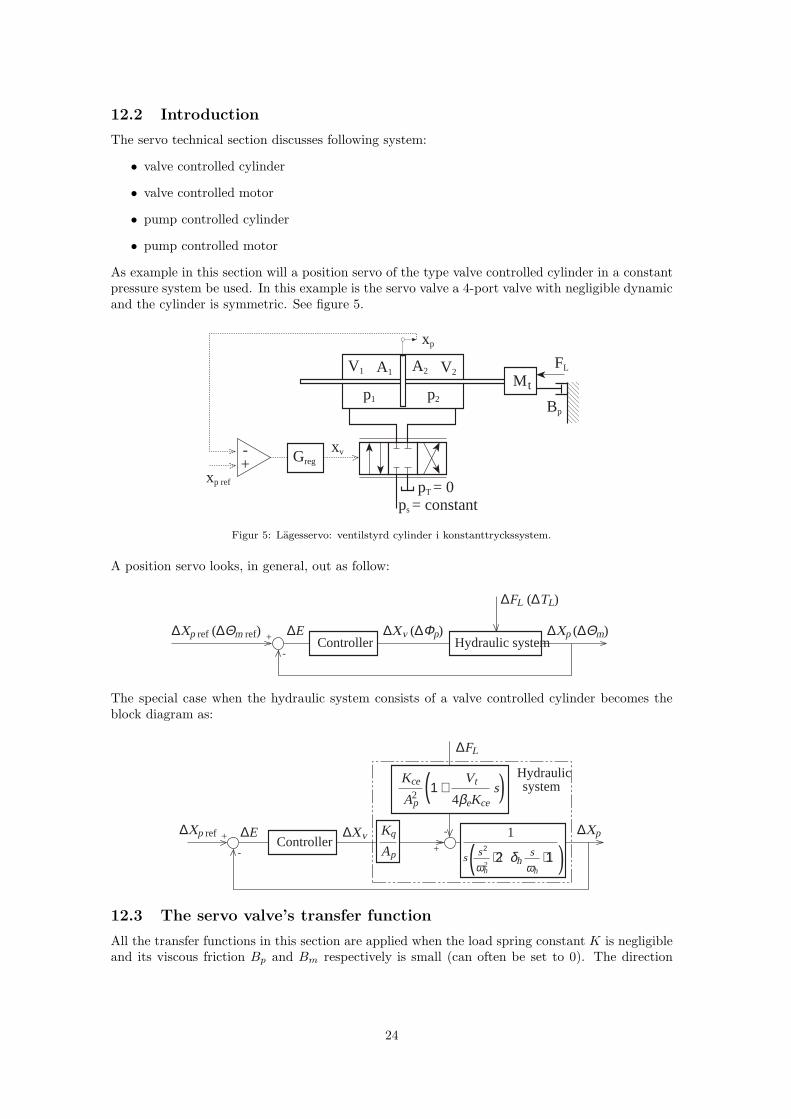
As example in this section will a position servo of the type valve controlled cylinder in a constantpressure system be used. In this example is the servo valve a 4-port valve with negligible dynamicand the cylinder is symmetric. See figure 5.

M t

FL

Bp

V1 A1

p1

A2 V2

p2

pT = 0ps = constant

xp

+-

xp ref

xvGreg

Figur 5: Lagesservo: ventilstyrd cylinder i konstanttryckssystem.

A position servo looks, in general, out as follow:

∆FL

∆E+

-

∆Xp ref (∆Θm ref)Controller Hydraulic system

∆Xp (∆Θm)∆Xv (∆Φp)

(∆TL)

The special case when the hydraulic system consists of a valve controlled cylinder becomes theblock diagram as:

∆FL

∆Xp

+

-∆Xv Kq

Ap

Kce

Ap2

Vt

4βeKce(1 + s)

Controller∆E+

-

∆Xp ref

Hydraulicsystem

1

+ 2δh + 1s

ωhωh2

s2s )(

12.3 The servo valve’s transfer function

All the transfer functions in this section are applied when the load spring constant K is negligibleand its viscous friction Bp and Bm respectively is small (can often be set to 0). The direction

24

dependent friction coefficient Cf is neglected also in the motor case.

Valve controlled systemsThe dynamic of the servo valve in the valve controlled systems is assumed to be negligible comparedto the system. Following is valid for the servo valve (see also section 12.4):

4-ports servo valve 3-ports servo valve

Kq =∂qL

∂xv

Kq =∂qL

∂xv

the servo valve’s flow gain

Kc = −∂qL

∂pL

Kc = −∂qL

∂pc

the servo valve’s flowpressure coefficient

Kp =Kq

Kc

=∂pL

∂xv

Kp =Kq

Kc

=∂pc

∂xv

the servo valve’s pressure gain

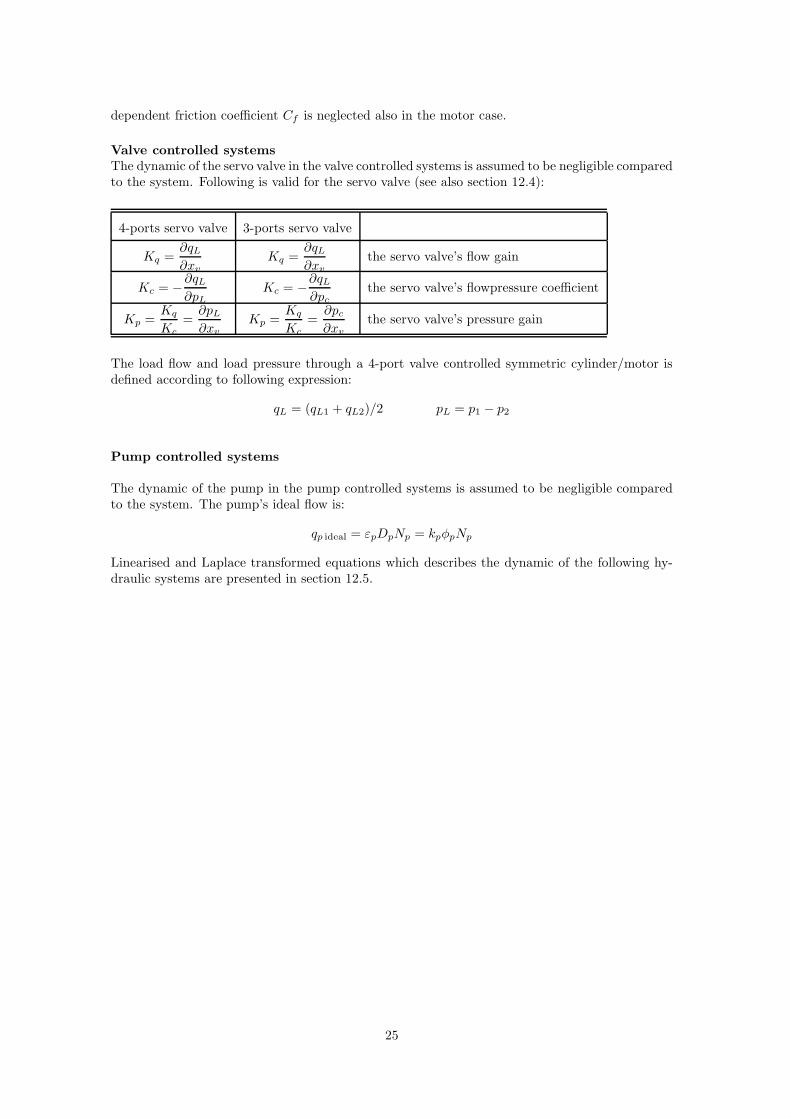
The load flow and load pressure through a 4-port valve controlled symmetric cylinder/motor isdefined according to following expression:

qL = (qL1 + qL2)/2 pL = p1 − p2

Pump controlled systems

The dynamic of the pump in the pump controlled systems is assumed to be negligible comparedto the system. The pump’s ideal flow is:

qp ideal = εpDpNp = kpφpNp

Linearised and Laplace transformed equations which describes the dynamic of the following hy-draulic systems are presented in section 12.5.

25

M t

FL

Bp

V1 A1

p1

A2 V2

p2

pT = 0ps = const

xp

xv

q1 q2

M t

FL

Bp

Vh Ah

pc

Ar

pT = 0ps = const

xp

xv

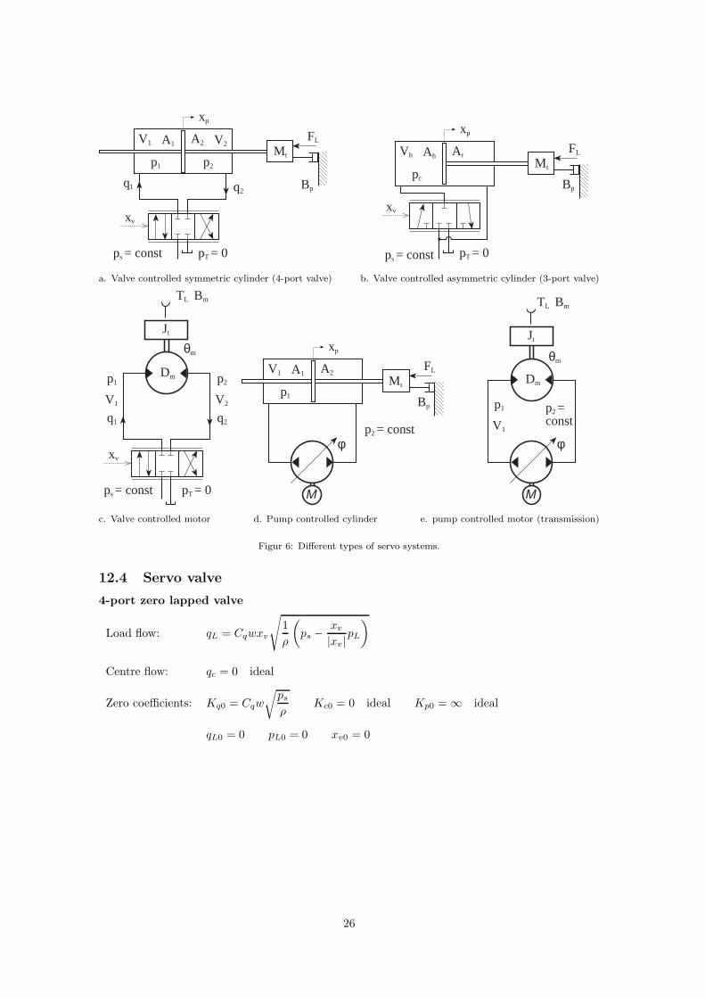
a. Valve controlled symmetric cylinder (4-port valve) b. Valve controlled asymmetric cylinder (3-port valve)

V1

p1

pT = 0ps = const

xv

TL Bm

θm

Dm

Jt

q1

V2

p2

q2

M t

FL

Bp

V1 A1

p1

A2

p2 = constφ

xp

M

V1

p1

TL Bm

θm

Dm

Jt

φ

M

p2 = const

c. Valve controlled motor d. Pump controlled cylinder e. pump controlled motor (transmission)

Figur 6: Different types of servo systems.

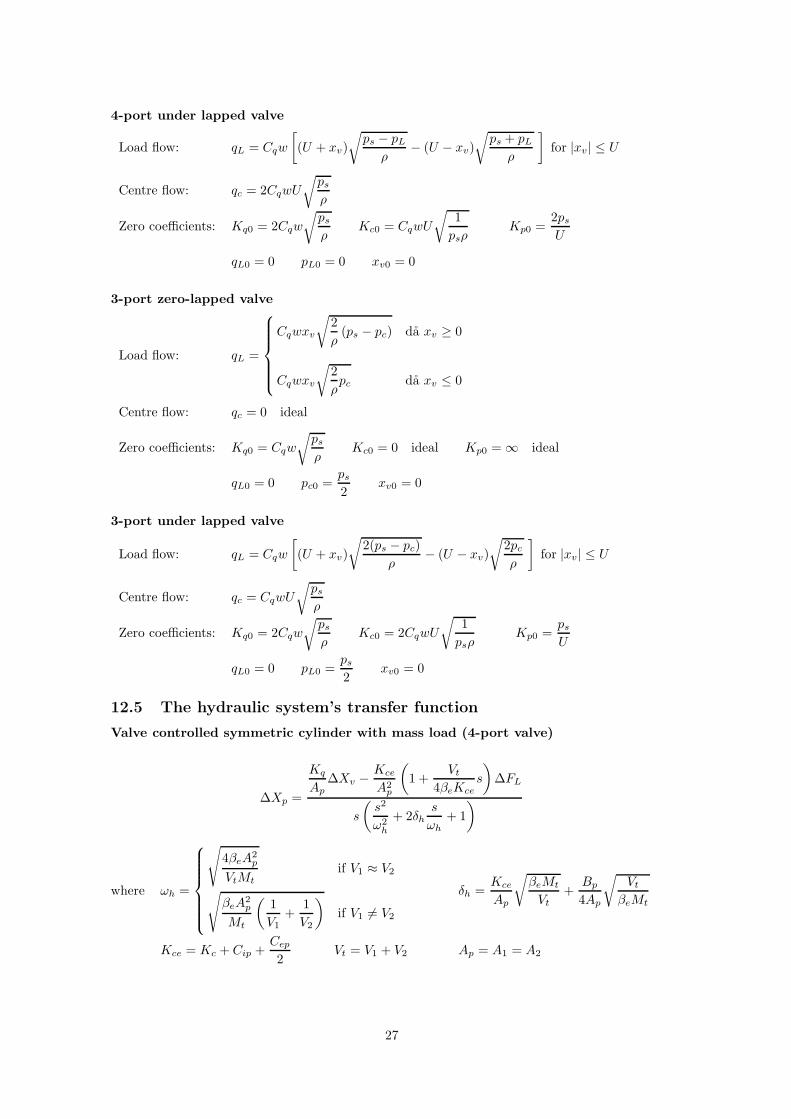
12.4 Servo valve

4-port zero lapped valve

Load flow: qL = Cqwxv

√

1

ρ

(

ps −xv

|xv|pL

)

Centre flow: qc = 0 ideal

Zero coefficients: Kq0 = Cqw

√

ps

ρKc0 = 0 ideal Kp0 = ∞ ideal

qL0 = 0 pL0 = 0 xv0 = 0

26

4-port under lapped valve

Load flow: qL = Cqw

[

(U + xv)

√

ps − pL

ρ− (U − xv)

√

ps + pL

ρ

]

for |xv| ≤ U

Centre flow: qc = 2CqwU

√

ps

ρ

Zero coefficients: Kq0 = 2Cqw

√

ps

ρKc0 = CqwU

√

1

psρKp0 =

2ps

U

qL0 = 0 pL0 = 0 xv0 = 0

3-port zero-lapped valve

Load flow: qL =

Cqwxv

√

2

ρ(ps − pc) da xv ≥ 0

Cqwxv

√

2

ρpc da xv ≤ 0

Centre flow: qc = 0 ideal

Zero coefficients: Kq0 = Cqw

√

ps

ρKc0 = 0 ideal Kp0 = ∞ ideal

qL0 = 0 pc0 =ps

2xv0 = 0

3-port under lapped valve

Load flow: qL = Cqw

[

(U + xv)

√

2(ps − pc)

ρ− (U − xv)

√

2pc

ρ

]

for |xv| ≤ U

Centre flow: qc = CqwU

√

ps

ρ

Zero coefficients: Kq0 = 2Cqw

√

ps

ρKc0 = 2CqwU

√

1

psρKp0 =

ps

U

qL0 = 0 pL0 =ps

2xv0 = 0

12.5 The hydraulic system’s transfer function

Valve controlled symmetric cylinder with mass load (4-port valve)

∆Xp =

Kq

Ap

∆Xv − Kce

A2p

(

1 +Vt

4βeKce

s

)

∆FL

s

(

s2

ω2h

+ 2δh

s

ωh

+ 1

)

where ωh =

√

4βeA2p

VtMt

if V1 ≈ V2

√

βeA2p

Mt

(

1

V1+

1

V2

)

if V1 6= V2

δh =Kce

Ap

√

βeMt

Vt

+Bp

4Ap

√

Vt

βeMt

Kce = Kc + Cip +Cep

2Vt = V1 + V2 Ap = A1 = A2

27

Valve controlled asymmetric cylinder with mass load (3-port valve)

∆Xp =

Kq

Ah

∆Xv − Kce

A2h

(

1 +Vh

βeKce

s

)

∆FL

s

(

s2

ω2h

+ 2δh

s

ωh

+ 1

)

where ωh =

√

βeA2h

VhMt

δh =Kce

2Ah

√

βeMt

Vh

+Bp

2Ah

√

Vh

βeMt

Kce = Kc + Cip

Valve controlled motor with moment of inertia

∆Θm =

Kq

Dm

∆Xv − Kce

D2m

(

1 +Vt

4βeKce

s

)

∆TL

s

(

s2

ω2h

+ 2δh

s

ωh

+ 1

)

where ωh =

√

4βeD2m

VtJt

δh =Kce

Dm

√

βeJt

Vt

+Bm

4Dm

√

Vt

βeJt

Kce = Kc + Cim +Cem

2Vt = V1 + V2, V1 = V2

Pump controlled cylinder with mass load

∆Xp =

kpNp

Ap

∆φp − Ct

A2p

(

1 +V0

βeCt

s

)

∆FL

s

(

s2

ω2h

+ 2δh

s

ωh

+ 1

)

where ωh =

√

βeA2p

V0Mt

δh =Ct

2Ap

√

βeMt

V0+

Bp

2Ap

√

V0

βeMt

V0 = V1 Ap = A1 = A2

Ct = Cit + Cet = Cip(iston) + Cip(ump) + Cep(iston) + Cep(ump)

Pump controlled motor with moment of inertia (transmission)

∆Θm =

kpNp

Dm

∆φp − Ct

D2m

(

1 +V0

βeCt

s

)

∆TL

s

(

s2

ω2h

+ 2δh

s

ωh

+ 1

)

where ωh =

√

βeD2m

V0Jt

δh =Ct

2Dm

√

βeJt

V0+

Bm

2Dm

√

V0

βeJt

V0 = V1 Ct = Cit + Cet = Cip + Cim + Cep + Cem

12.6 The servo stability

Feedback systems can become instable if the feedback is incorrect dimensioned. In this case westudy a position servo with proportional feedback Greg = Kreg. The open loop transfer functionbecome:

Au = GregGo =Kv

s

(

s2

ω2h

+ 2δh

s

ωh

+ 1

)

28

where Go is the transfer function which describes the hydraulic system’s output signal (cylinderposition) as function of the hydraulic system’s input signal (valve position) when the disturbancesignal (∆FL) is zero. The steady state loop gain Kv (also called the velocity coefficient) is:

Kv =Kq

Ap

Kreg valve controlled symmetric cylinder (4-port valve)

Kv =Kq

Ah

Kreg valve controlled asymmetric cylinder (3-port valve)

Kv =Kq

Dm

Kreg valve controlled motor

Kv =kpNp

Ap

Kreg pump controlled cylinder

Kv =kpNp

Dm

Kreg pump controlled motor

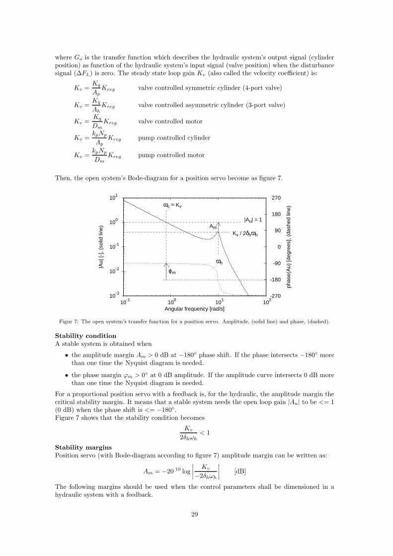
Then, the open system’s Bode-diagram for a position servo become as figure 7.

101

100

10-1

10-2

10-3

270

180

90

0

-90

-180

-27010210110010-1

Angular frequency [rad/s]

|Au|

[-],

(sol

id li

ne)

phas

e(A

u) [d

egre

es],

(das

hed

line)

|Au| = 1Am

Kv / 2δhωh

ϕm

ωc ≈ Kv

ωh

Figur 7: The open system’s transfer function for a position servo. Amplitude, (solid line) and phase, (dashed).

Stability conditionA stable system is obtained when

• the amplitude margin Am > 0 dB at −180◦ phase shift. If the phase intersects −180◦ morethan one time the Nyquist diagram is needed.

• the phase margin ϕm > 0◦ at 0 dB amplitude. If the amplitude curve intersects 0 dB morethan one time the Nyquist diagram is needed.

For a proportional position servo with a feedback is, for the hydraulic, the amplitude margin thecritical stability margin. It means that a stable system needs the open loop gain |Au| to be <= 1(0 dB) when the phase shift is <= −180◦.Figure 7 shows that the stability condition becomes

Kv

2δhωh

< 1

Stability marginsPosition servo (with Bode-diagram according to figure 7) amplitude margin can be written as:

Am = −20 10 log

∣

∣

∣

∣

Kv

−2δhωh

∣

∣

∣

∣

[dB]

The following margins should be used when the control parameters shall be dimensioned in ahydraulic system with a feedback.

29

amplitude margin: Am ≈ 10 dB

phase margin: ϕm ≥ 45◦

The system’s critical working conditionSince hydraulic systems are non-linear systems, the stability margin will become different indifferent working condition. From the figure for the open system’s transfer function Au thestability margin become worst when both ωh and δh are low and steady state loop gain Kv is big.This happened for a valve controlled symmetric cylinder when

• Cylinder piston is centered (xp = 0), i.e. V1 = V2 = Vt

2 . ωh is minimised.

• The servo valve is closed (xv = qL = 0), i.e. when Kc = Kc0. Kce and consequently δh isminimised.

• Cylinder piston is out balanced, i.e. when pL = 0. Kq, which is proportional to√

∆ps − ∆pL,is maximised and consequently also Kv (proportional to Kq).

With similar discussion, the critical working condition can be decided for other systems.In practical dimensioning, the hydraulic damping is often set to δh ≈ 0, 1.

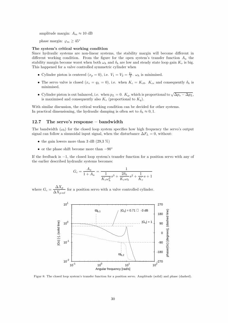
12.7 The servo’s response – bandwidth

The bandwidth (ωb) for the closed loop system specifies how high frequency the servo’s outputsignal can follow a sinusoidal input signal, when the disturbance ∆FL = 0, without:

• the gain lowers more than 3 dB (29,3 %)

• or the phase shift become more than −90◦

If the feedback is −1, the closed loop system’s transfer function for a position servo with any ofthe earlier described hydraulic systems becomes:

Gc =Au

1 + Au

=1

1

Kvω2h

s3 +2δh

Kvωh

s2 +1

Kv

s + 1

where Gc =∆Xp

∆Xp reffor a position servo with a valve controlled cylinder.

101

100

10-1

10-2

270

180

90

0

-90

-180

-27010210110010-1

Angular frequency [rad/s]

|Gc|

[-],

(sol

id li

ne)

phas

e(G

c) [d

egre

es],

(das

hed

line)

|Gc| = 1

|Gc| = 0.71 ⇔ -3 dBωb,1

ωb,2

Figur 8: The closed loop system’s transfer function for a position servo. Amplitude (solid) and phase (dashed).

30

The closed loop system’s transfer function can also be written as

Gc =1

(

s

ωb

+ 1

) (

s2

ω2nc

+ 2δnc

s

ωnc

+ 1

)

If δh and Kv/ωh is smallωnc ≈ ωh

ωb ≈ Kv

2δnc ≈ 2δh − Kv

ωh

12.8 The hydraulic system’s and the servo’s sensitivity to loading –stiffness

Cylinder - respective motor position sensitivity to disturbance force ∆FL or a disturbance torque∆TL is described with its stiffness S. When the stiffness is studied is all other input signalsassumed to be constant (∆Insignal = 0). The stiffness is defined as

S =∆FL

∆Xp

or S =∆TL

∆Θm

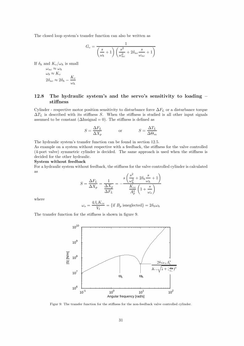
The hydraulic system’s transfer function can be found in section 12.5.As example on a system without respective with a feedback, the stiffness for the valve controlled(4-port valve) symmetric cylinder is decided. The same approach is used when the stiffness isdecided for the other hydraulic.System without feedbackFor a hydraulic system without feedback, the stiffness for the valve controlled cylinder is calculatedas

S =∆FL

∆Xp

=1

∆Xp

∆FL

= −s

(

s2

ω2h

+ 2δh

s

ωh

+ 1

)

Kce

A2p

(

1 +s

ωs

)

where

ωs =4βeKce

Vt

= {if Bp isneglected} = 2δhωh

The transfer function for the stiffness is shown in figure 9.

1010

109

108

107

106

10210110010-1

Angular frequency [rad/s]

|S| [

N/m

]

ωs ωh

2�h!hA2pKceq1 + (!h!s )2Figur 9: The transfer function for the stiffness for the non-feedback valve controlled cylinder.

31

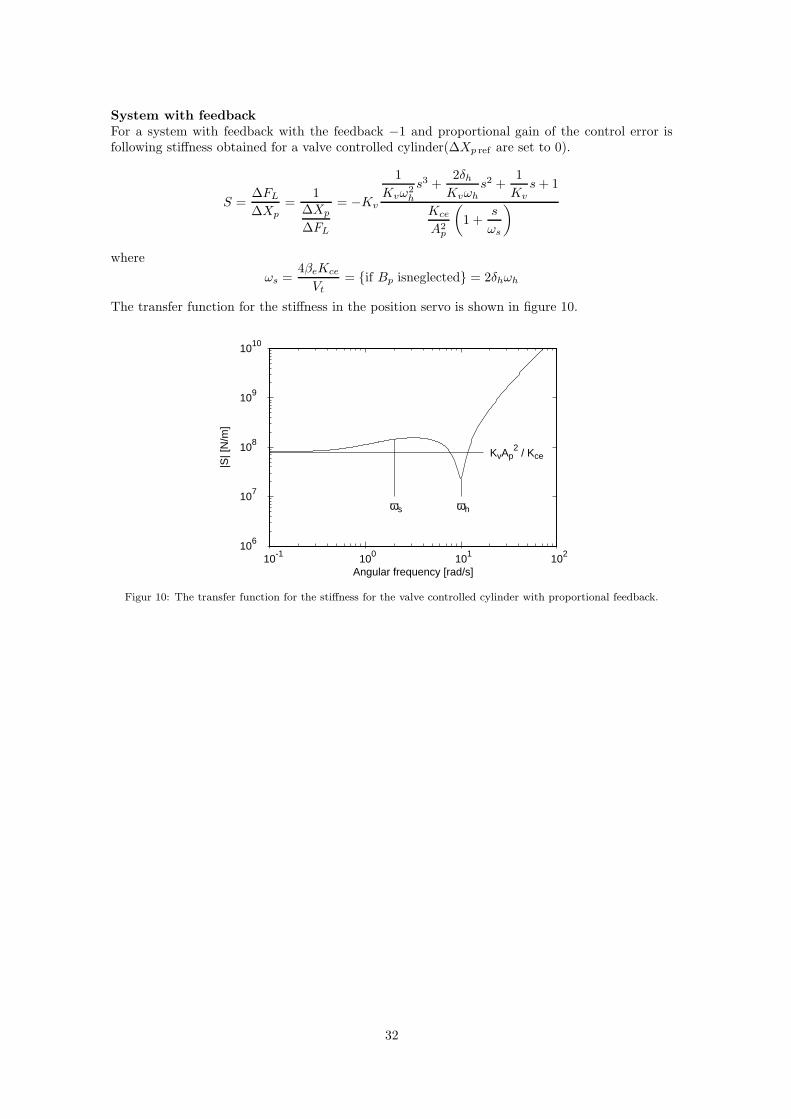
System with feedbackFor a system with feedback with the feedback −1 and proportional gain of the control error isfollowing stiffness obtained for a valve controlled cylinder(∆Xp ref are set to 0).

S =∆FL

∆Xp

=1

∆Xp

∆FL

= −Kv

1

Kvω2h

s3 +2δh

Kvωh

s2 +1

Kv

s + 1

Kce

A2p

(

1 +s

ωs

)

where

ωs =4βeKce

Vt

= {if Bp isneglected} = 2δhωh

The transfer function for the stiffness in the position servo is shown in figure 10.

1010

109

108

107

106

10210110010-1

Angular frequency [rad/s]

|S| [

N/m

]

ωs ωh

KvAp2 / Kce

Figur 10: The transfer function for the stiffness for the valve controlled cylinder with proportional feedback.

32

12.9 The servo’s steady state error

The control error e(t) in a servo system is defined as the difference between the output value andthe input value when ∆Disturbance signal = 0.According to end value theorem, the steady state control error will be:

ε0 = limt→∞

e(t) = lims→0

s∆E(s)

where the error gets the following expression if the feedback is −1:

∆E(s) = ∆Xpref − ∆Xp = ∆Xpref1

1 + Au

The end value theorem is only usable on an asymptotic stable system, i.e. if the output signalhas a finite limit value. For all systems can the transient be studied in the time domain (inversetransformation, see section 12.10).

The input signal is a stepIf the input signal ∆Xpref respective ∆Θmref is a step with the amplitude A becomes the inputsignal A/s in frequency domain. The end value theorem becomes

ε0 = lims→0

sA

s

1

1 + Au

=A

1 + lims→0

Au

→ A

∞ = 0

Practical, the steady state error does never become 0, because of the components which areincluded in the control loop do not have ideal characteristic.

The input signal is a rampIf the input signal ∆Xpref respective ∆Θmref is a ramp A · t (i.e. the speed A is desired), becomesthe input signal A/s2. The steady state position error becomes

ε0 = lims→0

sA

s2

1

1 + Au

=→ A

Kv

12.10 Control technical resources

Linearize

Non-linear differential equations are linearized around a working point with the first term of theTaylor series according to

∆f0

= ∆f(x10, x20, . . . , xn0) =

n∑

j=1

∆xj

∂f(x1, x2, . . . , xn)

∂xj (x10,x20,...,xn0)

where the working point is assumed to have stationary working conditions.

33

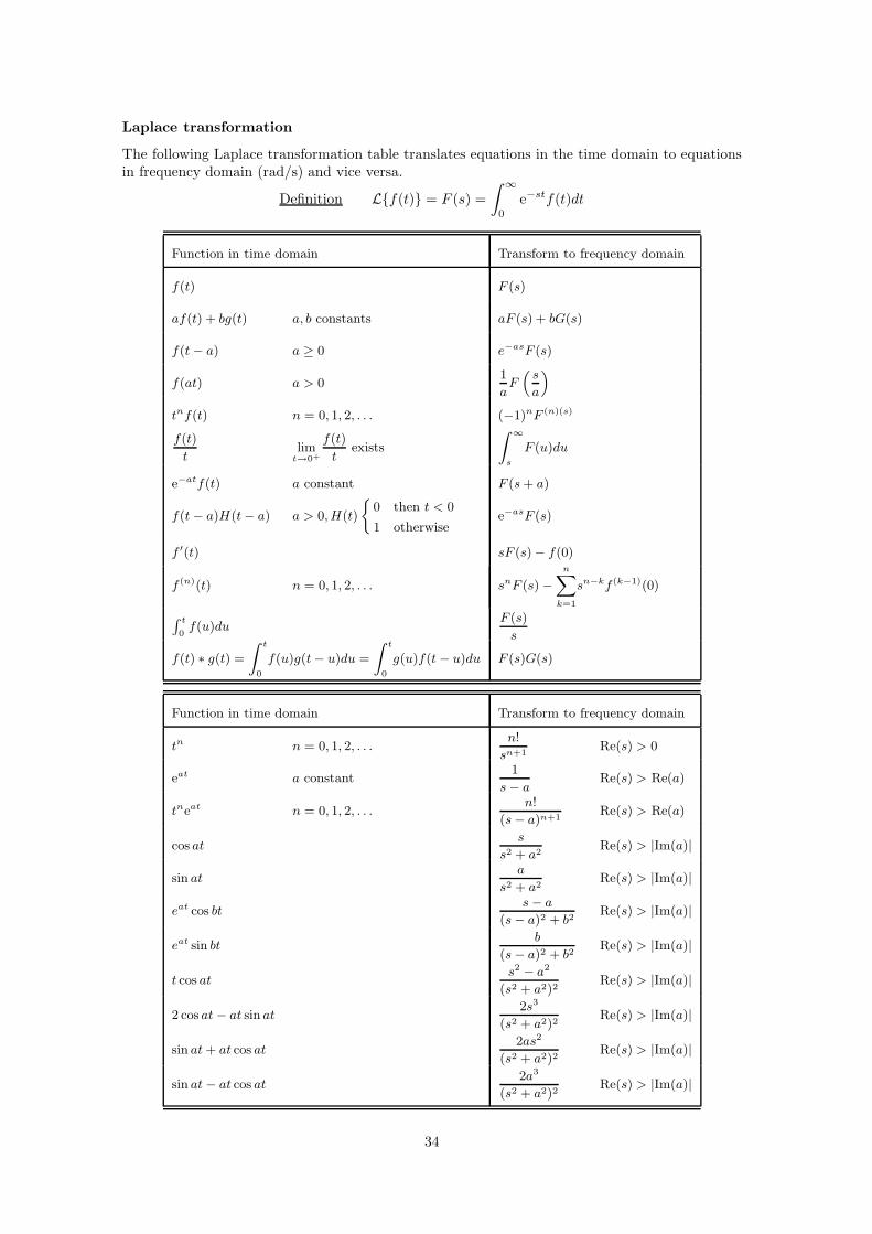
Laplace transformation

The following Laplace transformation table translates equations in the time domain to equationsin frequency domain (rad/s) and vice versa.

Definition L{f(t)} = F (s) =

∫ ∞

0

e−stf(t)dt

Function in time domain Transform to frequency domain

f(t) F (s)

af(t) + bg(t) a, b constants aF (s) + bG(s)

f(t − a) a ≥ 0 e−asF (s)

f(at) a > 01

aF

(

s

a

)

tnf(t) n = 0, 1, 2, . . . (−1)nF (n)(s)

f(t)

tlim

t→0+

f(t)

texists

∫ ∞

s

F (u)du

e−atf(t) a constant F (s + a)

f(t − a)H(t − a) a > 0, H(t)

{

0 then t < 0

1 otherwisee−asF (s)

f ′(t) sF (s) − f(0)

f (n)(t) n = 0, 1, 2, . . . snF (s) −

n∑

k=1

sn−kf (k−1)(0)

∫ t

0f(u)du

F (s)

s

f(t) ∗ g(t) =

∫ t

0

f(u)g(t − u)du =

∫ t

0

g(u)f(t − u)du F (s)G(s)

Function in time domain Transform to frequency domain

tn n = 0, 1, 2, . . .n!

sn+1Re(s) > 0

eat a constant1

s − aRe(s) > Re(a)

tneat n = 0, 1, 2, . . .n!

(s − a)n+1Re(s) > Re(a)

cos ats

s2 + a2Re(s) > |Im(a)|

sin ata

s2 + a2Re(s) > |Im(a)|

eat cos bts − a

(s − a)2 + b2Re(s) > |Im(a)|

eat sin btb

(s − a)2 + b2Re(s) > |Im(a)|

t cos ats2 − a2

(s2 + a2)2Re(s) > |Im(a)|

2 cos at − at sin at2s3

(s2 + a2)2Re(s) > |Im(a)|

sin at + at cos at2as2

(s2 + a2)2Re(s) > |Im(a)|

sin at − at cos at2a3

(s2 + a2)2Re(s) > |Im(a)|

34

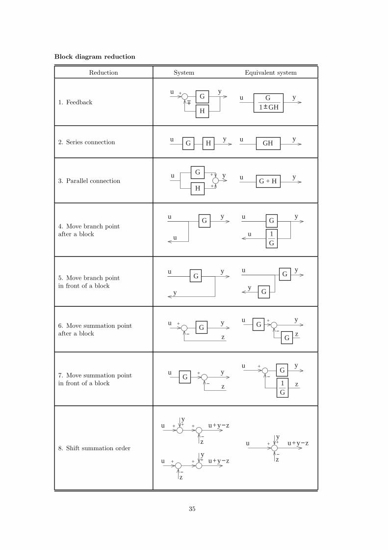
Block diagram reduction

Reduction System Equivalent system

1. Feedback1 GH

u yG±

+ Gu y

H

±

2. Series connection u yGH

u yHG

3. Parallel connectionu y

G + H+u y

H +

G

4. Move branch pointafter a block

u yG

u

u yG

G1u

5. Move branch pointin front of a block

u y

y

Gu y

G

yG

6. Move summation pointafter a block

u y

zG

+

−

u y

z

+

−G

G

7. Move summation pointin front of a block

u y

z

+

−G

G1

u y

z

+

−G

8. Shift summation order

uy

z

+

−

+ + u+y−z

uy

+ + u+y−z

z

+

−

uy

+ + u+y−z

z−

35

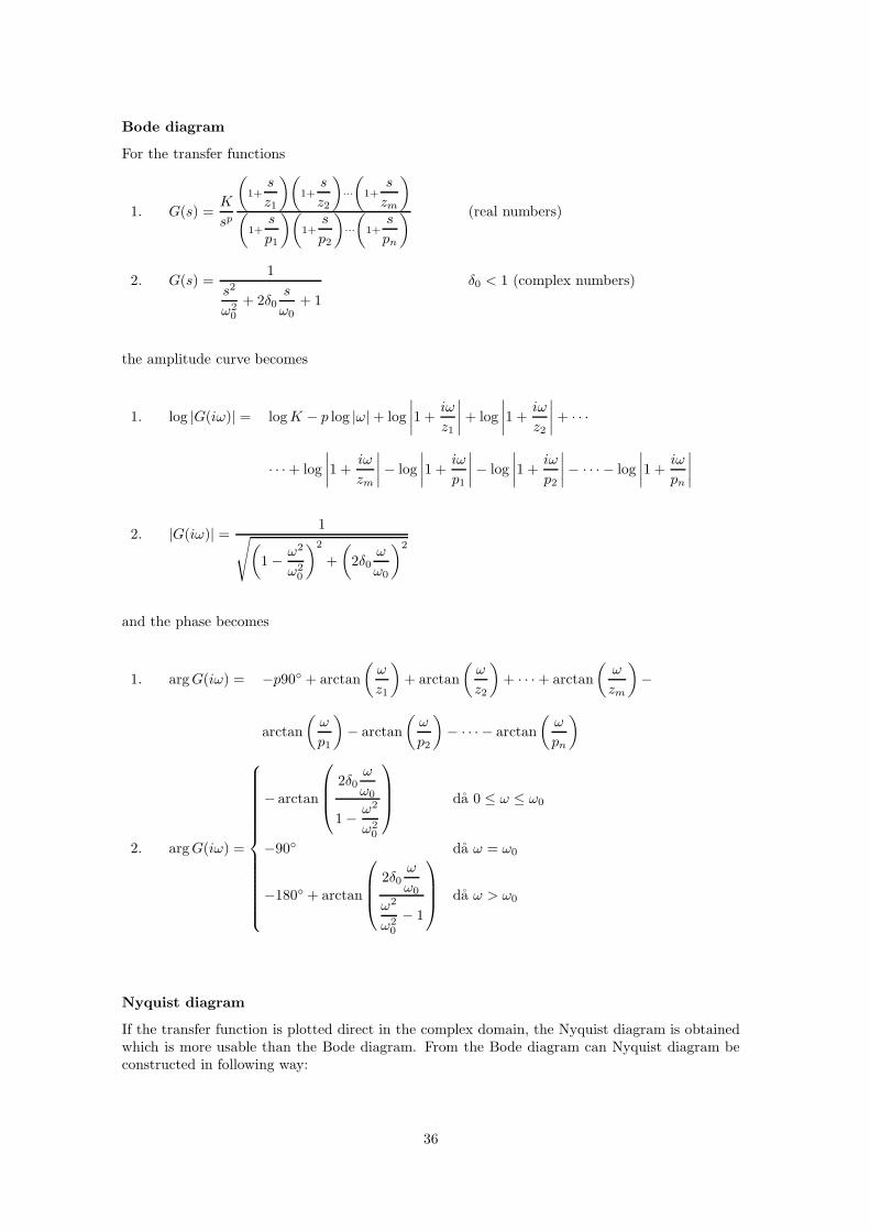
Bode diagram

For the transfer functions

1. G(s) =K

sp

(

1+s

z1

)(

1+s

z2

)

···

(

1+s

zm

)

(

1+s

p1

)(

1+s

p2

)

···

(

1+s

pn

) (real numbers)

2. G(s) =1

s2

ω20

+ 2δ0s

ω0+ 1

δ0 < 1 (complex numbers)

the amplitude curve becomes

1. log |G(iω)| = log K − p log |ω| + log

∣

∣

∣

∣

1 +iω

z1

∣

∣

∣

∣

+ log

∣

∣

∣

∣

1 +iω

z2

∣

∣

∣

∣

+ · · ·

· · · + log

∣

∣

∣

∣

1 +iω

zm

∣

∣

∣

∣

− log

∣

∣

∣

∣

1 +iω

p1

∣

∣

∣

∣

− log

∣

∣

∣

∣

1 +iω

p2

∣

∣

∣

∣

− · · · − log

∣

∣

∣

∣

1 +iω

pn

∣

∣

∣

∣

2. |G(iω)| =1

√

(

1 − ω2

ω20

)2

+

(

2δ0ω

ω0

)2

and the phase becomes

1. arg G(iω) = −p90◦ + arctan

(

ω

z1

)

+ arctan

(

ω

z2

)

+ · · · + arctan

(

ω

zm

)

−

arctan

(

ω

p1

)

− arctan

(

ω

p2

)

− · · · − arctan

(

ω

pn

)

2. arg G(iω) =

− arctan

2δ0ω

ω0

1 − ω2

ω20

da 0 ≤ ω ≤ ω0

−90◦ da ω = ω0

−180◦ + arctan

2δ0ω

ω0

ω2

ω20

− 1

da ω > ω0

Nyquist diagram

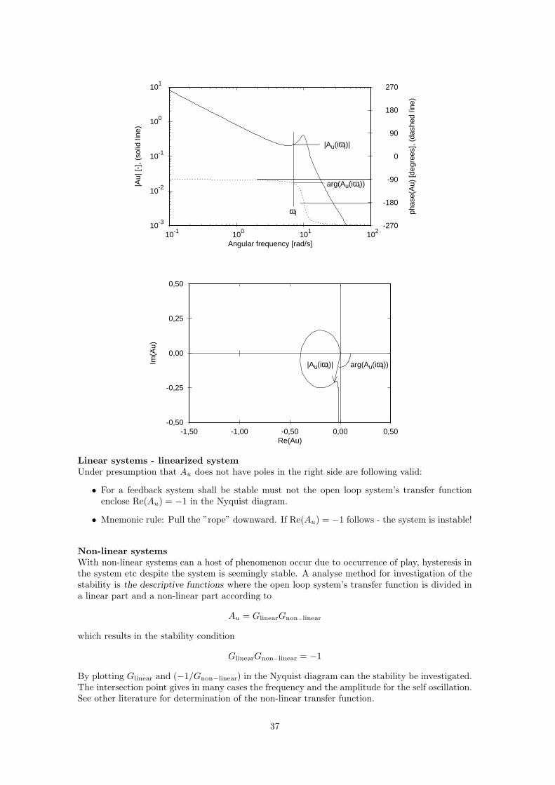
If the transfer function is plotted direct in the complex domain, the Nyquist diagram is obtainedwhich is more usable than the Bode diagram. From the Bode diagram can Nyquist diagram beconstructed in following way:

36

101

100

10-1

10-2

10-3

270

180

90

0

-90

-180

-27010210110010-1

Angular frequency [rad/s]

|Au|

[-],

(sol

id li

ne)

phas

e(A

u) [d

egre

es],

(das

hed

line)

|Au(iωi)|

arg(Au(iωi))

ωi

0,50

0,25

0,00

-0,25

-0,500,500,00-0,50-1,00-1,50

Re(Au)

Im(A

u)

|Au(iωi)| arg(Au(iωi))

Linear systems - linearized systemUnder presumption that Au does not have poles in the right side are following valid:

• For a feedback system shall be stable must not the open loop system’s transfer functionenclose Re(Au) = −1 in the Nyquist diagram.

• Mnemonic rule: Pull the ”rope” downward. If Re(Au) = −1 follows - the system is instable!

Non-linear systemsWith non-linear systems can a host of phenomenon occur due to occurrence of play, hysteresis inthe system etc despite the system is seemingly stable. A analyse method for investigation of thestability is the descriptive functions where the open loop system’s transfer function is divided ina linear part and a non-linear part according to

Au = GlinearGnon−linear

which results in the stability condition

GlinearGnon−linear = −1

By plotting Glinear and (−1/Gnon−linear) in the Nyquist diagram can the stability be investigated.The intersection point gives in many cases the frequency and the amplitude for the self oscillation.See other literature for determination of the non-linear transfer function.

37

13 Hydraulic fluids

13.1 NomenclatureV :volume [m3]V1 :start volume (secant) [m3]V2 :end volume (secant) [m3]Vc :volume (reservoir) [m3]Vg :volume (gas) [m3]Vℓ :volume (fluid) [m3]Vt :total volume [m3]p :absolute pressure [Pa]p0 :absolute pressure at NTP (= 0,1 MPa) [Pa]p1 :start pressure (secant) [Pa]p2 :end pressure (secant) [Pa]u :flow velocity in x-led [m/s]n :polytrophic exponent [-]ys :correction coefficient (secant) [-]yt :correction coefficient (tangent) [-]

x0 :amount of air in the oil(gas volume/total volume atnormal state, NTP) [-]

ν :kinematic viscosity [m2/s]ρ :density [kg/m3]βe :effective bulk modulus [Pa]βc :bulk modulus (reservoir) [Pa]βg :bulk modulus (gas) [Pa]βℓ :bulk modulus (fluid) [Pa]βt :bulk modulus with no air in the oil (tangent) [Pa]βs :bulk modulus with no air in the olja (secant) [Pa]βbt :bulk modulus with air in the oil (tangent) [Pa]βbs :bulk modulus with air in the oil (secant) [Pa]τ :skjuvspanning [N/m2]η :dynamic viscosity [Ns/m2]

Definition, ηdynamic viscosityfor Newton fluid

τ = ηdu

dy

y

x

u(y)

Kinematic viscosity ν =η

ρ

Bulk modulus for oil with no air

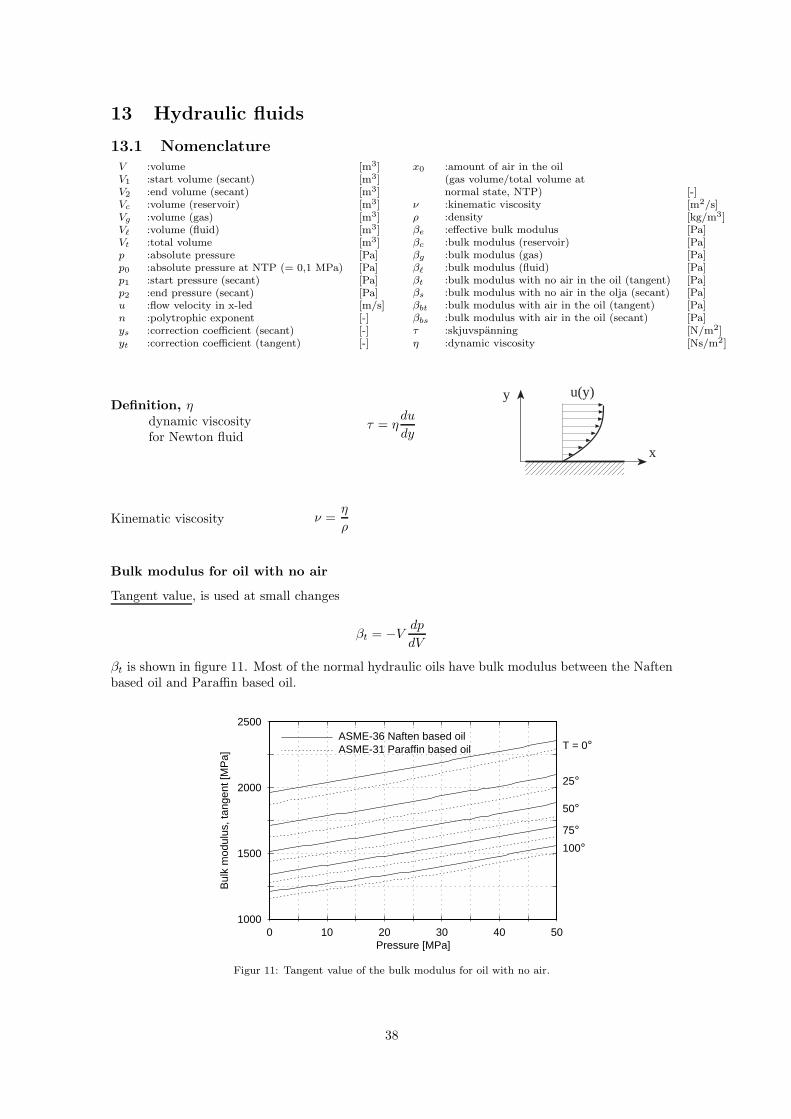
Tangent value, is used at small changes

βt = −Vdp

dV

βt is shown in figure 11. Most of the normal hydraulic oils have bulk modulus between the Naftenbased oil and Paraffin based oil.

2500

2000

1500

100050403020100

Pressure [MPa]

Bul

k m

odul

us, t

ange

nt [M

Pa]

T = 0°

25°

50°

75°100°

ASME-36 Naften based oilASME-31 Paraffin based oil

Figur 11: Tangent value of the bulk modulus for oil with no air.

38

Secant value, is used at big changes from normal pressure(p1 = 0, V1) till (p2, V2)

βs = −V1p2

V2 − V1

βs is shown in figure 12. Most of the normal hydraulic oils have bulk modulus between the Naftenbase oil and Paraffin base oil.

2500

2000

1500

100050403020100

Pressure [MPa]

Bul

k m

odul

us, s

ecan

t [M

Pa]

T = 0°

25°

50°

75°100°

ASME-36 Naften based oilASME-31 Paraffin based oil

Figur 12: Secant value of bulk modulus for oil with no air.

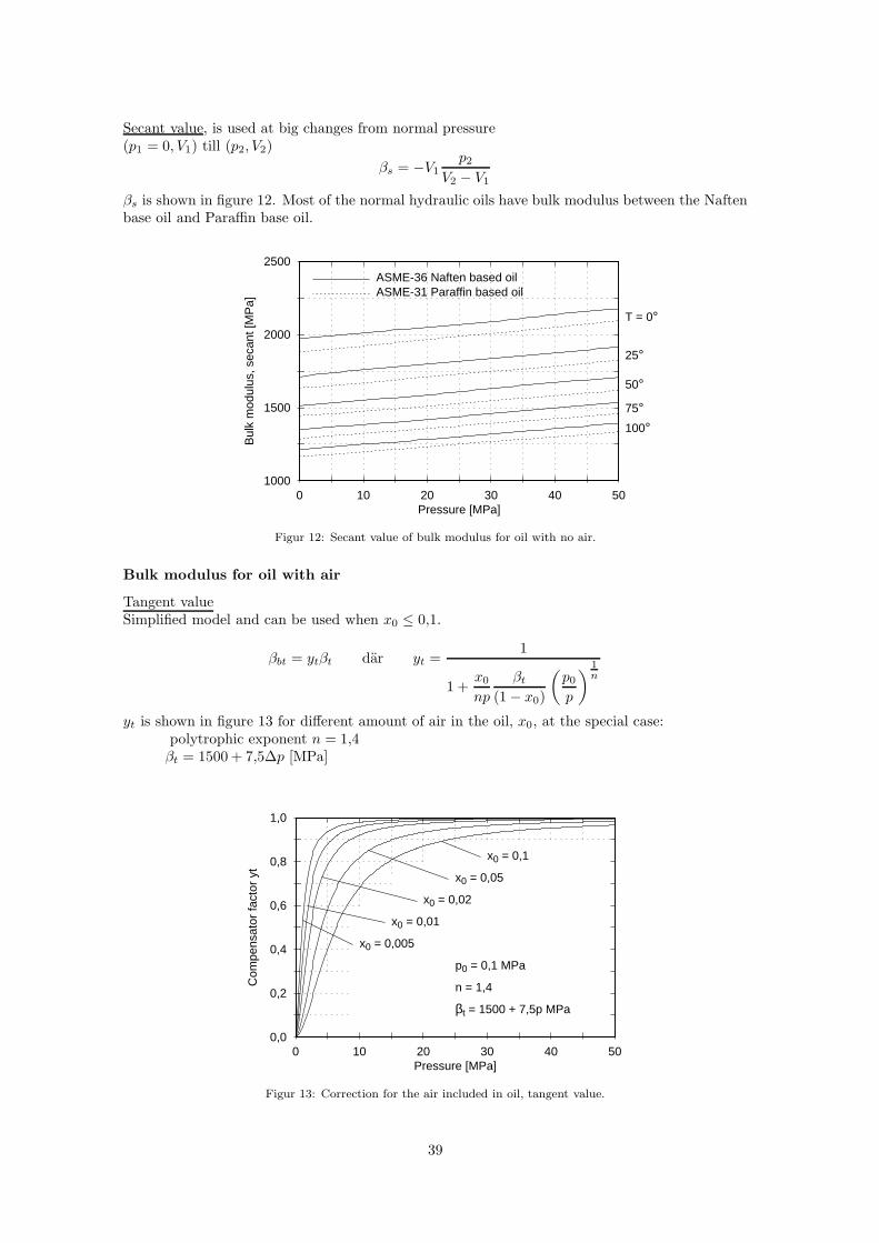
Bulk modulus for oil with air

Tangent valueSimplified model and can be used when x0 ≤ 0,1.

βbt = ytβt dar yt =1

1 +x0

np

βt

(1 − x0)

(

p0

p

)

1n

yt is shown in figure 13 for different amount of air in the oil, x0, at the special case:polytrophic exponent n = 1,4βt = 1500 + 7,5∆p [MPa]

1,0

0,8

0,6

0,4

0,2

0,050403020100

Pressure [MPa]

Com

pens

ator

fact

or y

t

x0 = 0,005

x0 = 0,01

x0 = 0,02

x0 = 0,05

x0 = 0,1

p0 = 0,1 MPa

n = 1,4

βt = 1500 + 7,5p MPa

Figur 13: Correction for the air included in oil, tangent value.

39

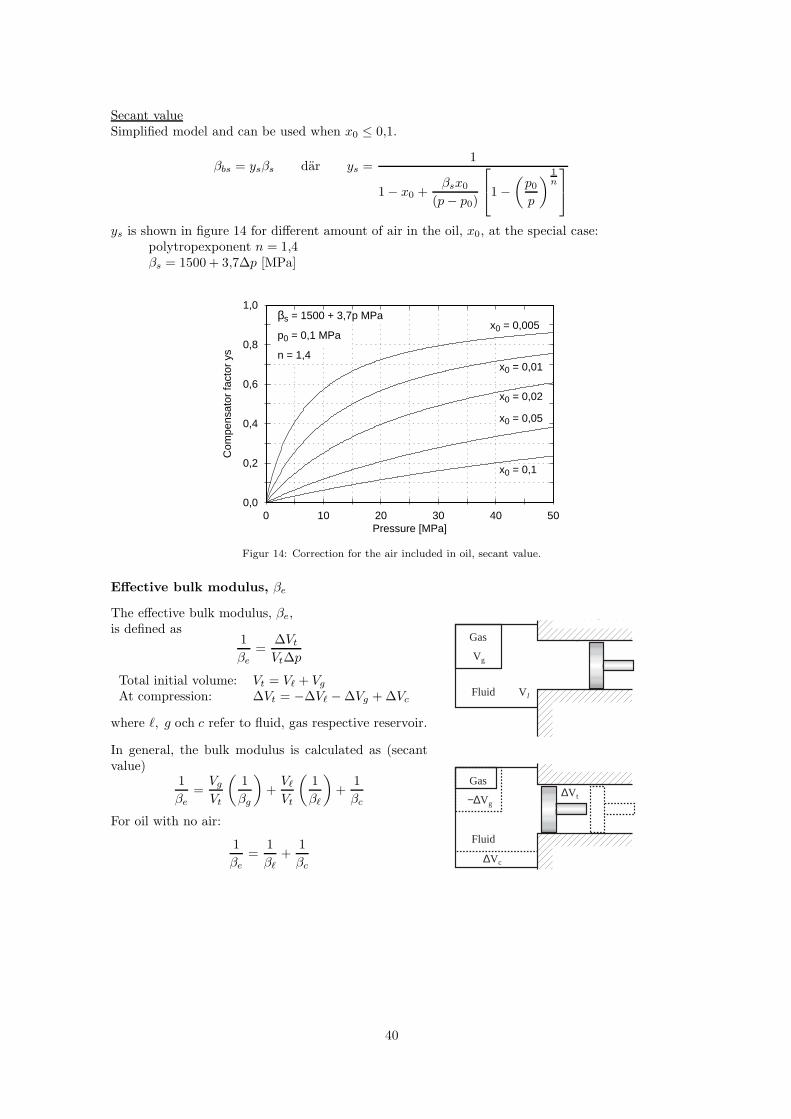
Secant valueSimplified model and can be used when x0 ≤ 0,1.

βbs = ysβs dar ys =1

1 − x0 +βsx0

(p − p0)

1 −(

p0

p

)

1n

ys is shown in figure 14 for different amount of air in the oil, x0, at the special case:polytropexponent n = 1,4βs = 1500 + 3,7∆p [MPa]

1,0

0,8

0,6

0,4

0,2

0,050403020100

Pressure [MPa]

Com

pens

ator

fact

or y

s

x0 = 0,005

x0 = 0,01

x0 = 0,02

x0 = 0,05

x0 = 0,1

p0 = 0,1 MPa

n = 1,4

βs = 1500 + 3,7p MPa

Figur 14: Correction for the air included in oil, secant value.

Effective bulk modulus, βe

The effective bulk modulus, βe,is defined as

1

βe

=∆Vt

Vt∆p

Total initial volume: Vt = Vℓ + Vg

At compression: ∆Vt = −∆Vℓ − ∆Vg + ∆Vc

where ℓ, g och c refer to fluid, gas respective reservoir.

In general, the bulk modulus is calculated as (secantvalue)

1

βe

=Vg

Vt

(

1

βg

)

+Vℓ

Vt

(

1

βℓ

)

+1

βc

For oil with no air:

1

βe

=1

βℓ

+1

βc

Gas

−∆Vg∆V t

∆Vc

Fluid

Gas

Vg

V lFluid

40

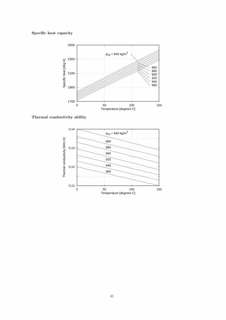
Specific heat capacity

2500

2300

2100

1900

1700150100500

Temperature [degrees C]

Spe

cific

hea

t [J/

kg K

]

ρ20 = 840 kg/m3

860 880 900 920 940 960

Thermal conductivity ability

0,14

0,13

0,12

0,11150100500

Temperature [degrees C]

The

rmal

con

duct

ivity

[W/m

K]

ρ20 = 840 kg/m3

860

880

900

920

940

960

41

14 Pneumatic

14.1 NomenclatureA0 :min. cross-section area of the orifice [m2]A12 :effective entrance area [m2]A23 :effective exit area [m2]Ae :effective orifice area (CdA0) [m2]Cd :flow coefficient [-]Ci :C-value for component i [-]Cs :C-value for system [-]

K :constant [√

kgK/J]

Kt :temperature correction (√

T0/T1) [-]

N :parameter [-]R :gas constant (287 for air) [J/kg K]T0 :reference temperature (NTP) [K]T1 :upstream total temperature [K]T3 :downstream total temperature [K]Tv :total temperature i volume [K]

b :critical pressure ratio [-]bi :b-value for component i [-]bs :b-value for system [-]m :mass flow [kg/s]p1 :upstream total absolute pressure

(= static + dynamic pressure) [Pa]p2 :downstream static absolute pressure [Pa]p3 :atmospheric pressure (0,1 MPa) [Pa]pv :atmospheric pressure in volume [Pa]q :volume flow [m3/s]t :time [s]α :parameter [-]κ :isentropic exponent [-]ω :parameter [-]

τ :dimension free time (=√

RT AtV

) [-]

14.2 Stream through nozzle

According to the thermodynamic, the mass flow m through a nozzle can be written as

m =p1CdA0KN√

T1

where K =

√

√

√

√

√κ

R

(

2

κ + 1

)

κ + 1

κ − 1

N =

1 forp2

p1≤

(

p2

p1

)∗

√

√

√

√

√

√

√

√

√

√

(

p2

p1

)

2

κ−

(

p2

p1

)

κ + 1

κ

κ − 1

2

(

2

κ + 1

)

κ + 1

κ − 1

forp2

p1>

(

p2

p1

)∗

critical pressure ratio: b =

(

p2

p1

)∗

=

(

2

κ + 1

)

κ

κ − 1

With b- and C-value hold for volume flow q following expression at NTP

q = p1KtCω

ω =

1 forp2

p1≤ b

√

√

√

√

√

√

1 −

p2

p1− b

1 − b

2

forp2

p1> b

42

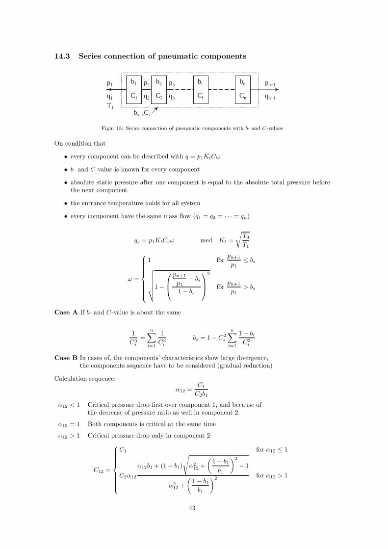
14.3 Series connection of pneumatic components

bn

Cn

pn+1

qn+1

p1

q1

b1

C1

p2

q2

b2

C2

p3

q3

bi

Ci

T1bs ,Cs

Figur 15: Series connection of pneumatic components with b- and C-values

On condition that

• every component can be described with q = p1KtCω

• b- and C-value is known for every component

• absolute static pressure after one component is equal to the absolute total pressure beforethe next component

• the entrance temperature holds for all system

• every component have the same mass flow (q1 = q2 = · · · = qn)

qs = p1KtCsω med Kt =

√

T0

T1

ω =

1 forpn+1

p1≤ bs

√

√

√

√

√

√

1 −

pn+1

p1− bs

1 − bs

2

forpn+1

p1> bs

Case A If b- and C-value is about the same

1

C3s

=

n∑

i=1

1

C3i

bs = 1 − C2s

n∑

i=1

1 − bi

C2i

Case B In cases of, the components’ characteristics show large divergence,the components sequence have to be considered (gradual reduction)

Calculation sequence:

α12 =C1

C2b1

α12 < 1 Critical pressure drop first over component 1, and because ofthe decrease of pressure ratio as well in component 2.

α12 = 1 Both components is critical at the same time

α12 > 1 Critical pressure drop only in component 2

C12 =

C1 for α12 ≤ 1

C2α12

α12b1 + (1 − b1)

√

α212 +

(

1 − b1

b1

)2

− 1

α212 +

(

1 − b1

b1

)2 for α12 > 1

43

b12 = 1 − C212

(

1 − b1

C21

+1 − b2

C22

)

{

α13 =C12

C3b12osv . . .

}

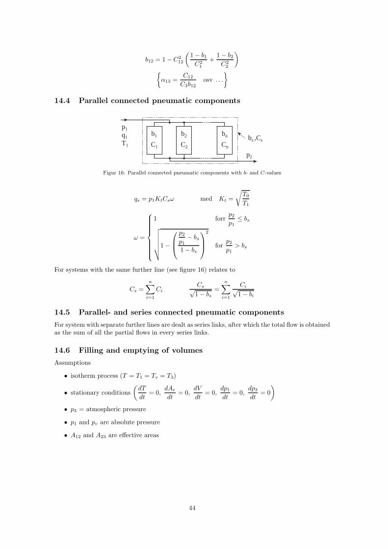
14.4 Parallel connected pneumatic components

b1

C1

p1

q1b2

C2T1

bs ,Cs

p2

bn

Cn

Figur 16: Parallel connected pneumatic components with b- and C-values

qs = p1KtCsω med Kt =

√

T0

T1

ω =

1 forrp2

p1≤ bs

√

√

√

√

√

√

1 −

p2

p1− bs

1 − bs

2

forp2

p1> bs

For systems with the same further line (see figure 16) relates to

Cs =n

∑

i=1

Ci

Cs√1 − bs

=n

∑

i=1

Ci√1 − bi

14.5 Parallel- and series connected pneumatic components

For system with separate further lines are dealt as series links, after which the total flow is obtainedas the sum of all the partial flows in every series links.

14.6 Filling and emptying of volumes

Assumptions

• isotherm process (T = T1 = Tv = T3)

• stationary conditions

(

dT

dt= 0,

dAe

dt= 0,

dV

dt= 0,

dp1

dt= 0,

dp3

dt= 0

)

• p3 = atmospheric pressure

• p1 and pv are absolute pressure

• A12 and A23 are effective areas

44

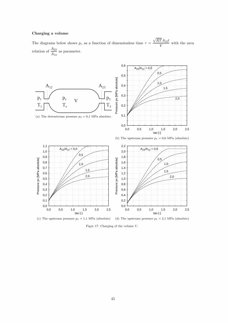
Charging a volume

The diagrams below shows pv as a function of dimensionless time τ =

√RTA12t

Vwith the area

relation ofA23

A12as parameter.

Vp1

A12

T1

pv

Tv

p3

T3

A23

(a) The downstream pressure p3 = 0,1 MPa absolute.

0,6

0,5

0,4

0,3

0,2

0,1

0,02,52,01,51,00,50,0

tao [-]

Pre

ssur

e pv

[MP

a ab

solu

te]

A23/A12 = 0,0

0,5

1,0

1,5

2,0

(b) The upstream pressure p1 = 0,6 MPa (absolute)

1,1

1,0

0,9

0,8

0,7

0,6

0,5

0,4

0,3

0,2

0,1

0,02,52,01,51,00,50,0

tao [-]

Pre

ssur

e pv

[MP

a ab

solu

te]

A23/A12 = 0,0

0,5

1,0

1,5

2,0

(c) The upstream pressure p1 = 1,1 MPa (absolute)

2,2

2,0

1,8

1,6

1,4

1,2

1,0

0,8

0,6

0,4

0,2

0,02,52,01,51,00,50,0

tao [-]

Pre

ssur

e pv

[MP

a ab

solu

te]

A23/A12 = 0,0

0,5

1,0

1,5

2,0

(d) The upstream pressure p1 = 2,1 MPa (absolute)

Figur 17: Charging of the volume V .

45

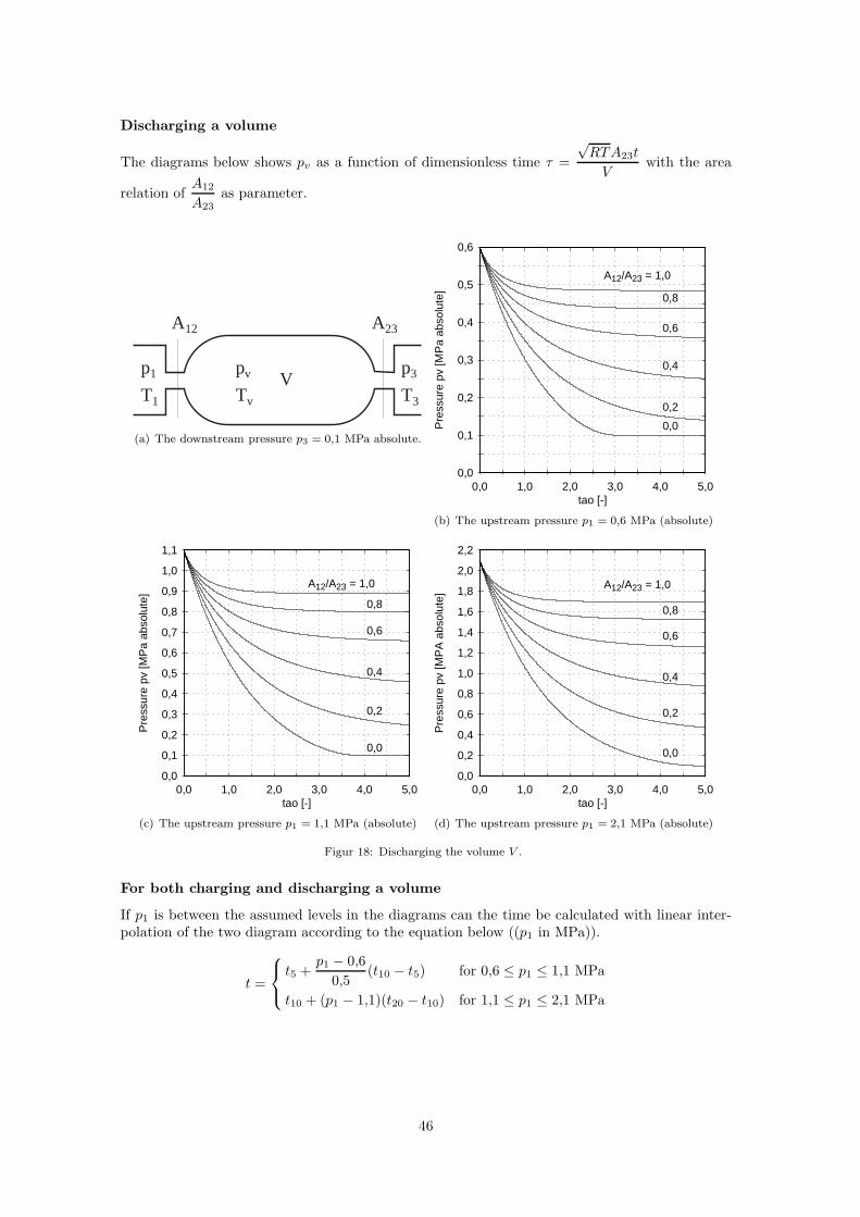
Discharging a volume

The diagrams below shows pv as a function of dimensionless time τ =

√RTA23t

Vwith the area

relation ofA12

A23as parameter.

Vp1

A12

T1

pv

Tv

p3

T3

A23

(a) The downstream pressure p3 = 0,1 MPa absolute.

0,6

0,5

0,4

0,3

0,2

0,1

0,05,04,03,02,01,00,0

tao [-]

Pre

ssur

e pv

[MP

a ab

solu

te]

A12/A23 = 1,0

0,8

0,6

0,4

0,2

0,0

(b) The upstream pressure p1 = 0,6 MPa (absolute)

1,1

1,0

0,9

0,8

0,7

0,6

0,5

0,4

0,3

0,2

0,1

0,05,04,03,02,01,00,0

tao [-]

Pre

ssur

e pv

[MP

a ab

solu

te]

A12/A23 = 1,0

0,8

0,6

0,4

0,2

0,0

(c) The upstream pressure p1 = 1,1 MPa (absolute)

2,2

2,0

1,8

1,6

1,4

1,2

1,0

0,8

0,6

0,4

0,2

0,05,04,03,02,01,00,0

tao [-]

Pre

ssur

e pv

[MP

A a

bsol

ute]

A12/A23 = 1,0

0,8

0,6

0,4

0,2

0,0

(d) The upstream pressure p1 = 2,1 MPa (absolute)

Figur 18: Discharging the volume V .

For both charging and discharging a volume

If p1 is between the assumed levels in the diagrams can the time be calculated with linear inter-polation of the two diagram according to the equation below ((p1 in MPa)).

t =

t5 +p1 − 0,6

0,5(t10 − t5) for 0,6 ≤ p1 ≤ 1,1 MPa

t10 + (p1 − 1,1)(t20 − t10) for 1,1 ≤ p1 ≤ 2,1 MPa

46

Appendix A

Symbols for hydraulic diagrams

Correspond to the international standard CETOP RP3 and the Swedish SMS 712. It is specifiedwhen the two standards differ.

General symbols................................................................... 48Mechanical elements............................................................. 48Pipes and connections.......................................................... 48Control systems.................................................................... 49Pumps and Motors............................................................... 49Cylinders.............................................................................. 51Directional control valves..................................................... 52Check valves or non-return valves........................................ 53Pressure control valves................................´....................... 54Flow control valves............................................................... 55Components for cooling, filtering, energy storage etc.......... 56Energy sources..................................................................... 57Measurement equipments..................................................... 57

47

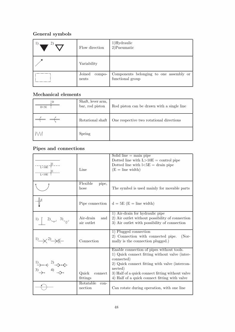
General symbols

1) 2)

Flow direction1)Hydraulic2)Pneumatic

Variability

Joined compo-nents

Components belonging to one assembly orfunctional group

Mechanical elements

D

D<5E

Shaft, lever arm,bar, rod piston Rod piston can be drawn with a single line

Rotational shaft One respective two rotational directions

Spring

Pipes and connections

E

L<10E

E

L<10E

Line

Solid line = main pipeDotted line with L>10E = control pipeDotted line with l<5E = drain pipe(E = line width)

Flexible pipe,hose The symbol is used mainly for movable parts

d

Pipe connection d = 5E (E = line width)

1) 2) 3) Air-drain andair outlet

1) Air-drain for hydraulic pipe2) Air outlet without possibility of connection3) Air outlet with possibility of connection

1) 2)Connection

1) Plugged connection2) Connection with connected pipe. (Nor-mally is the connection plugged.)

1) 2)

3) 4)Quick connectfittings

Enable connection of pipes without tools.1) Quick connect fitting without valve (inter-connected)2) Quick connect fitting with valve (intercon-nected)3) Half of a quick connect fitting without valve4) Half of a quick connect fitting with valve

Rotatable con-nection Can rotate during operation, with one line

48

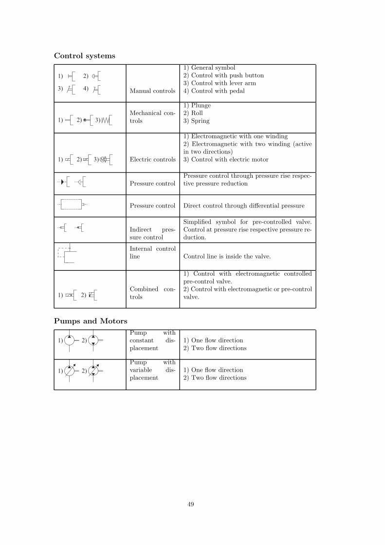
Control systems

1) 2)

3) 4) Manual controls

1) General symbol2) Control with push button3) Control with lever arm4) Control with pedal

1) 2) 3)Mechanical con-trols

1) Plunge2) Roll3) Spring

1) 2) 3) M Electric controls

1) Electromagnetic with one winding2) Electromagnetic with two winding (activein two directions)3) Control with electric motor

Pressure controlPressure control through pressure rise respec-tive pressure reduction

Pressure control Direct control through differential pressure

Indirect pres-sure control

Simplified symbol for pre-controlled valve.Control at pressure rise respective pressure re-duction.

Internal controlline Control line is inside the valve.

1) 2)Combined con-trols

1) Control with electromagnetic controlledpre-control valve.2) Control with electromagnetic or pre-controlvalve.

Pumps and Motors

1) 2)

Pump withconstant dis-placement

1) One flow direction2) Two flow directions

1) 2)

Pump withvariable dis-placement

1) One flow direction2) Two flow directions

49

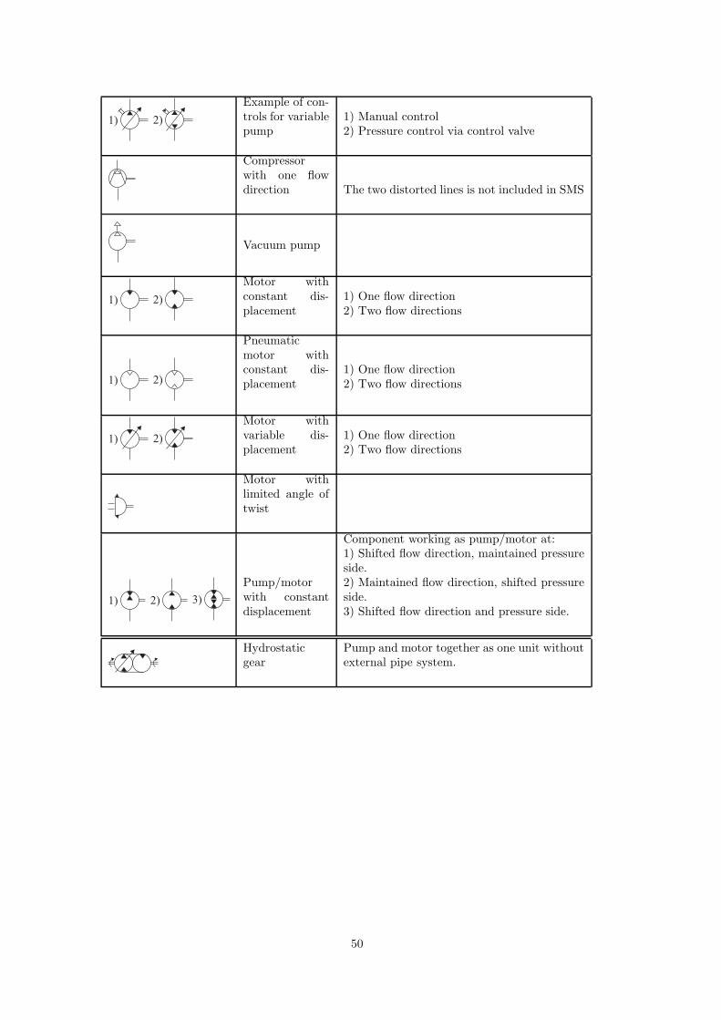
1) 2)

Example of con-trols for variablepump

1) Manual control2) Pressure control via control valve

Compressorwith one flowdirection The two distorted lines is not included in SMS

Vacuum pump

1) 2)

Motor withconstant dis-placement

1) One flow direction2) Two flow directions

1) 2)

Pneumaticmotor withconstant dis-placement

1) One flow direction2) Two flow directions

1) 2)

Motor withvariable dis-placement

1) One flow direction2) Two flow directions

Motor withlimited angle oftwist

1) 2) 3)

Pump/motorwith constantdisplacement

Component working as pump/motor at:1) Shifted flow direction, maintained pressureside.2) Maintained flow direction, shifted pressureside.3) Shifted flow direction and pressure side.

Hydrostaticgear

Pump and motor together as one unit withoutexternal pipe system.

50

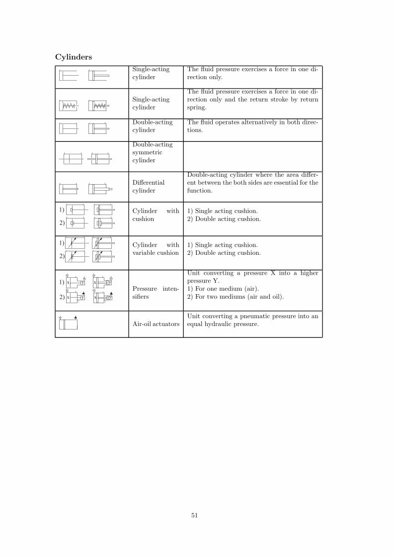
Cylinders

Single-actingcylinder

The fluid pressure exercises a force in one di-rection only.

Single-actingcylinder

The fluid pressure exercises a force in one di-rection only and the return stroke by returnspring.

Double-actingcylinder

The fluid operates alternatively in both direc-tions.

Double-actingsymmetriccylinder

Differentialcylinder

Double-acting cylinder where the area differ-ent between the both sides are essential for thefunction.

1)

2)

Cylinder withcushion

1) Single acting cushion.2) Double acting cushion.

1)

2)

Cylinder withvariable cushion

1) Single acting cushion.2) Double acting cushion.

1)

2) x y

x y x y

x y

Pressure inten-sifiers

Unit converting a pressure X into a higherpressure Y.1) For one medium (air).2) For two mediums (air and oil).

Air-oil actuatorsUnit converting a pneumatic pressure into anequal hydraulic pressure.

51

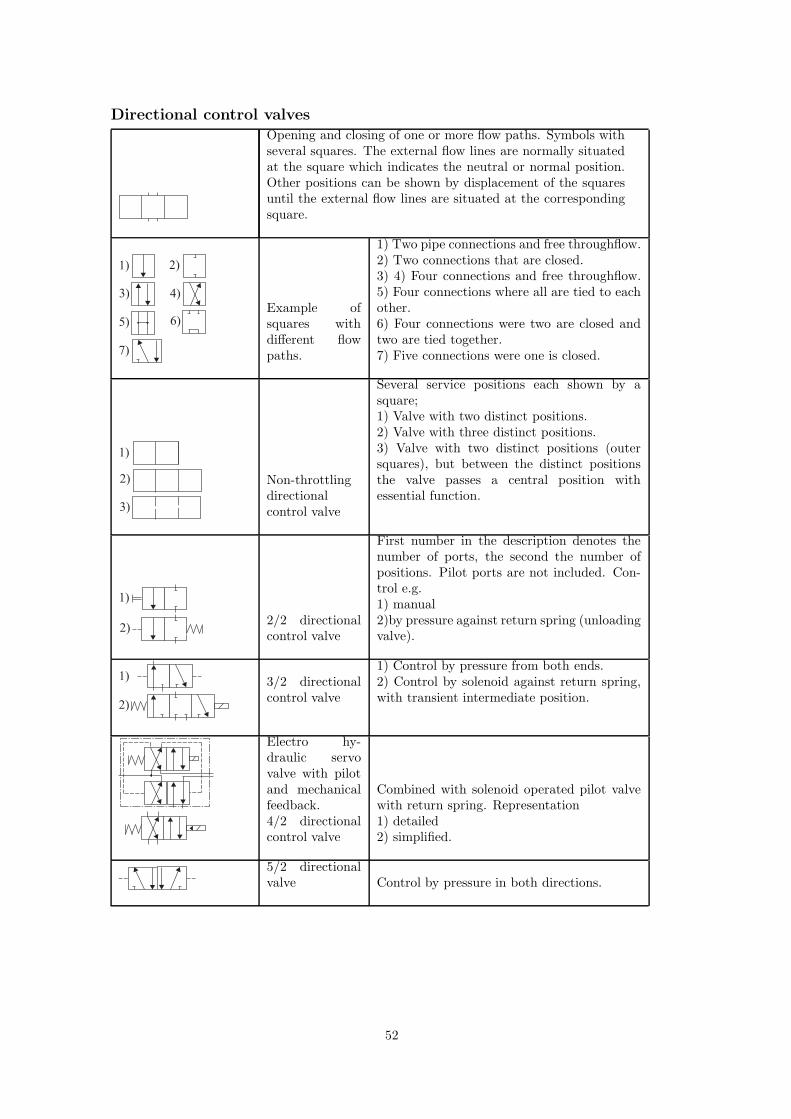
Directional control valvesOpening and closing of one or more flow paths. Symbols withseveral squares. The external flow lines are normally situatedat the square which indicates the neutral or normal position.Other positions can be shown by displacement of the squaresuntil the external flow lines are situated at the correspondingsquare.

1)

3)

5)

2)

4)

6)

7)

Example ofsquares withdifferent flowpaths.

1) Two pipe connections and free throughflow.2) Two connections that are closed.3) 4) Four connections and free throughflow.5) Four connections where all are tied to eachother.6) Four connections were two are closed andtwo are tied together.7) Five connections were one is closed.

1)

2)

3)

Non-throttlingdirectionalcontrol valve

Several service positions each shown by asquare;1) Valve with two distinct positions.2) Valve with three distinct positions.3) Valve with two distinct positions (outersquares), but between the distinct positionsthe valve passes a central position withessential function.

1)

2)2/2 directionalcontrol valve

First number in the description denotes thenumber of ports, the second the number ofpositions. Pilot ports are not included. Con-trol e.g.1) manual2)by pressure against return spring (unloadingvalve).

1)

2)

3/2 directionalcontrol valve

1) Control by pressure from both ends.2) Control by solenoid against return spring,with transient intermediate position.

Electro hy-draulic servovalve with pilotand mechanicalfeedback.4/2 directionalcontrol valve

Combined with solenoid operated pilot valvewith return spring. Representation1) detailed2) simplified.

5/2 directionalvalve Control by pressure in both directions.

52

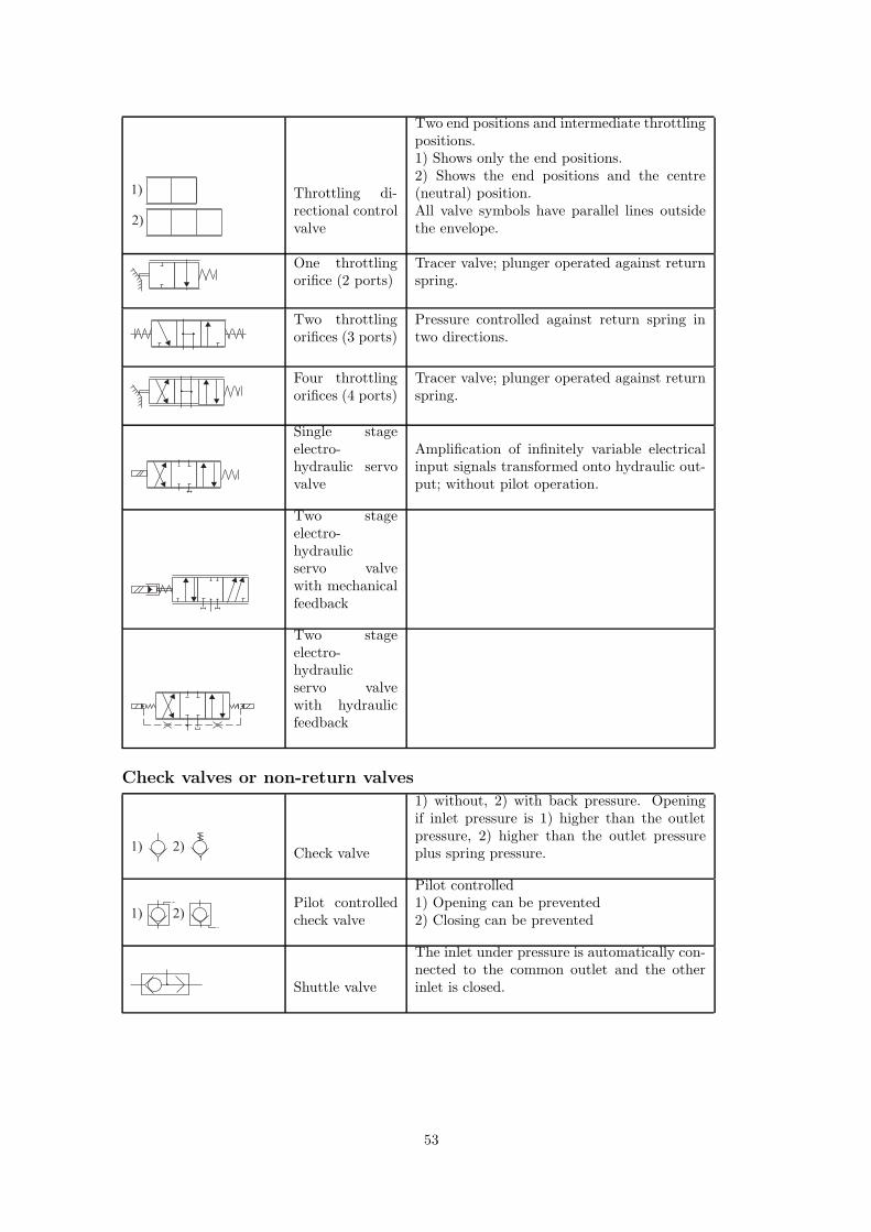
1)

2)

Throttling di-rectional controlvalve

Two end positions and intermediate throttlingpositions.1) Shows only the end positions.2) Shows the end positions and the centre(neutral) position.All valve symbols have parallel lines outsidethe envelope.

One throttlingorifice (2 ports)

Tracer valve; plunger operated against returnspring.

Two throttlingorifices (3 ports)

Pressure controlled against return spring intwo directions.

Four throttlingorifices (4 ports)

Tracer valve; plunger operated against returnspring.

Single stageelectro-hydraulic servovalve

Amplification of infinitely variable electricalinput signals transformed onto hydraulic out-put; without pilot operation.

Two stageelectro-hydraulicservo valvewith mechanicalfeedback

Two stageelectro-hydraulicservo valvewith hydraulicfeedback

Check valves or non-return valves

1) 2) Check valve

1) without, 2) with back pressure. Openingif inlet pressure is 1) higher than the outletpressure, 2) higher than the outlet pressureplus spring pressure.

1) 2)Pilot controlledcheck valve

Pilot controlled1) Opening can be prevented2) Closing can be prevented

Shuttle valve

The inlet under pressure is automatically con-nected to the common outlet and the otherinlet is closed.

53

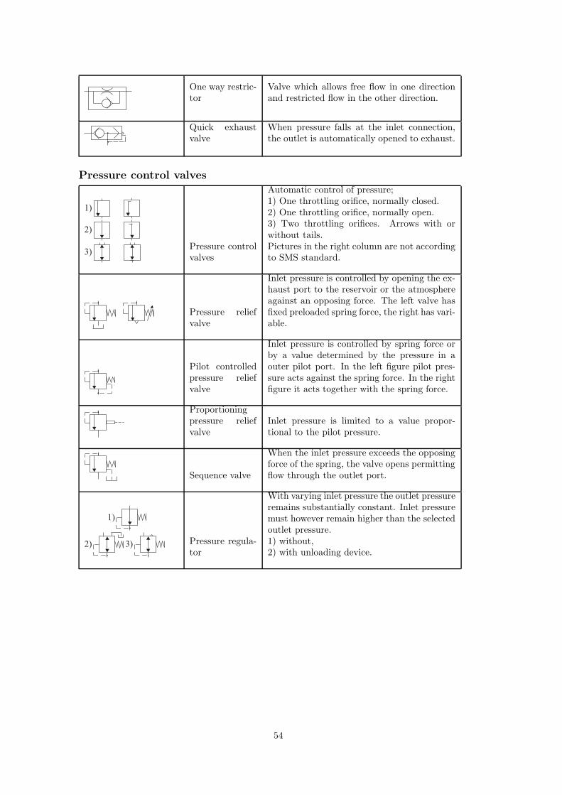
One way restric-tor

Valve which allows free flow in one directionand restricted flow in the other direction.

Quick exhaustvalve

When pressure falls at the inlet connection,the outlet is automatically opened to exhaust.

Pressure control valves

1)

3)

2)

Pressure controlvalves

Automatic control of pressure;1) One throttling orifice, normally closed.2) One throttling orifice, normally open.3) Two throttling orifices. Arrows with orwithout tails.Pictures in the right column are not accordingto SMS standard.

Pressure reliefvalve

Inlet pressure is controlled by opening the ex-haust port to the reservoir or the atmosphereagainst an opposing force. The left valve hasfixed preloaded spring force, the right has vari-able.

Pilot controlledpressure reliefvalve

Inlet pressure is controlled by spring force orby a value determined by the pressure in aouter pilot port. In the left figure pilot pres-sure acts against the spring force. In the rightfigure it acts together with the spring force.

Proportioningpressure reliefvalve

Inlet pressure is limited to a value propor-tional to the pilot pressure.

Sequence valve

When the inlet pressure exceeds the opposingforce of the spring, the valve opens permittingflow through the outlet port.

1)

3)2) Pressure regula-tor

With varying inlet pressure the outlet pressureremains substantially constant. Inlet pressuremust however remain higher than the selectedoutlet pressure.1) without,2) with unloading device.

54

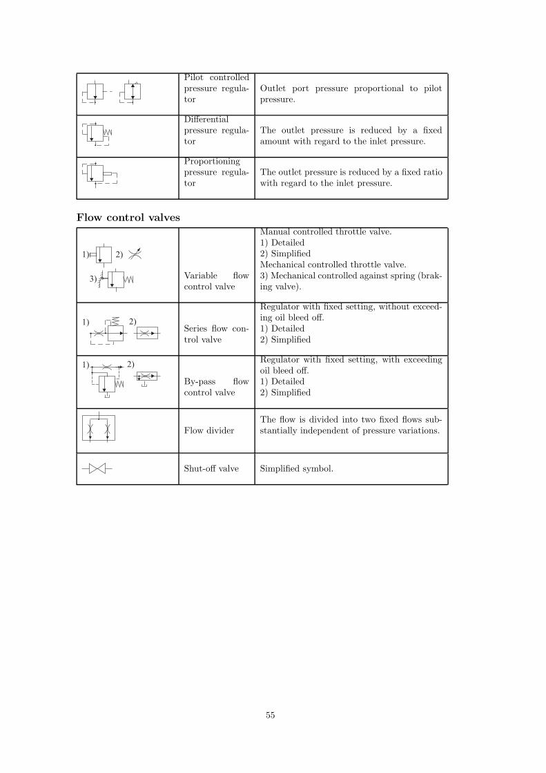
Pilot controlledpressure regula-tor

Outlet port pressure proportional to pilotpressure.

Differentialpressure regula-tor

The outlet pressure is reduced by a fixedamount with regard to the inlet pressure.

Proportioningpressure regula-tor

The outlet pressure is reduced by a fixed ratiowith regard to the inlet pressure.

Flow control valves

1)

3)

2)

Variable flowcontrol valve

Manual controlled throttle valve.1) Detailed2) SimplifiedMechanical controlled throttle valve.3) Mechanical controlled against spring (brak-ing valve).

1) 2)Series flow con-trol valve

Regulator with fixed setting, without exceed-ing oil bleed off.1) Detailed2) Simplified

1) 2)

By-pass flowcontrol valve

Regulator with fixed setting, with exceedingoil bleed off.1) Detailed2) Simplified

Flow dividerThe flow is divided into two fixed flows sub-stantially independent of pressure variations.

Shut-off valve Simplified symbol.

55

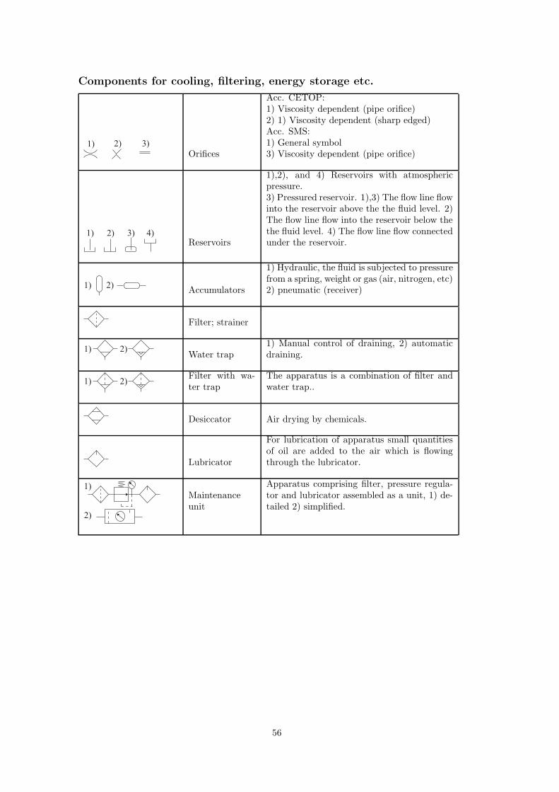
Components for cooling, filtering, energy storage etc.

1) 2) 3)

Orifices

Acc. CETOP:1) Viscosity dependent (pipe orifice)2) 1) Viscosity dependent (sharp edged)Acc. SMS:1) General symbol3) Viscosity dependent (pipe orifice)

1) 2) 3) 4)Reservoirs

1),2), and 4) Reservoirs with atmosphericpressure.3) Pressured reservoir. 1),3) The flow line flowinto the reservoir above the the fluid level. 2)The flow line flow into the reservoir below thethe fluid level. 4) The flow line flow connectedunder the reservoir.

1) 2)Accumulators

1) Hydraulic, the fluid is subjected to pressurefrom a spring, weight or gas (air, nitrogen, etc)2) pneumatic (receiver)

Filter; strainer

1) 2)Water trap

1) Manual control of draining, 2) automaticdraining.

1) 2)Filter with wa-ter trap

The apparatus is a combination of filter andwater trap..

Desiccator Air drying by chemicals.

Lubricator

For lubrication of apparatus small quantitiesof oil are added to the air which is flowingthrough the lubricator.

1)

2)

Maintenanceunit

Apparatus comprising filter, pressure regula-tor and lubricator assembled as a unit, 1) de-tailed 2) simplified.

56

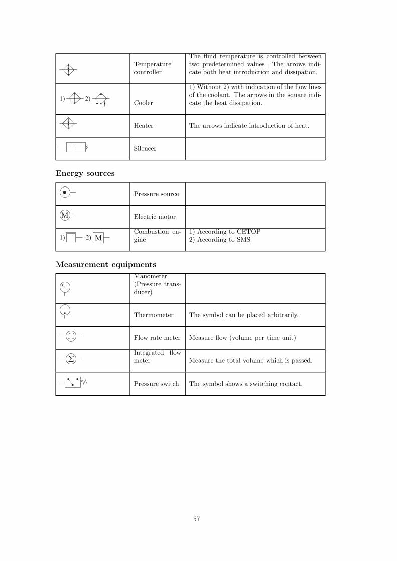
Temperaturecontroller

The fluid temperature is controlled betweentwo predetermined values. The arrows indi-cate both heat introduction and dissipation.

1) 2)Cooler

1) Without 2) with indication of the flow linesof the coolant. The arrows in the square indi-cate the heat dissipation.

Heater The arrows indicate introduction of heat.

Silencer

Energy sources

Pressure source

Μ Electric motor

1) 2) ΜCombustion en-gine

1) According to CETOP2) According to SMS

Measurement equipments

Manometer(Pressure trans-ducer)

Thermometer The symbol can be placed arbitrarily.

Flow rate meter Measure flow (volume per time unit)

ΣIntegrated flowmeter Measure the total volume which is passed.

Pressure switch The symbol shows a switching contact.

57