sensors

Article

Deep Generative Models-Based Anomaly Detectionfor Spacecraft Control Systems

Hyojung Ahn 1, Dawoon Jung 1 and Han-Lim Choi 2,*1 Korea Aerospace Research Institute, Daejeon 34133, Korea; hjahn@kari.re.kr (H.A.); dwjung@kari.re.kr (D.J.)2 Department of Aerospace Engineering, Korea Advanced Institute of Science and Technology,

Daejeon 341141, Korea* Correspondence: hanlimc@kaist.ac.kr

Received: 1 March 2020; Accepted: 30 March 2020; Published: 2 April 2020�����������������

Abstract: A spacecraft attitude control system provides mechanical and electrical control to achievethe required functions under various mission scenarios. Although generally designed to be highlyreliable, mission failure can occur if anomalies occur and the attitude control system fails to properlyorient and stabilize the spacecraft. Because accessing spacecraft to directly repair such problemsis usually infeasible, developing a continuous condition monitoring model is necessary to detectanomalies and respond accordingly. In this study, a method for detecting anomalies and characterizingfailures for spacecraft attitude control systems is proposed. Herein, features are extracted frommultidimensional time-series data of a simulation of the attitude control system. Then, the artificialneural network learning algorithms based on two types of generation models are applied. A Bayesianoptimization algorithm with a Gaussian process is used to optimize the hyperparameters for the neuralnetwork to improve the performance. The performance is evaluated based on the reconstruction errorthrough the algorithm using the newly generated data not used for learning as input data. Resultsshow that the detection performance depends on the operating characteristics of each submode in theoperation scenarios and type of generation model. The diagnostic results are monitored to detectanomalies in operation modes and scenarios.

Keywords: anomaly detection; spacecraft; attitude control system; deep-learning; generative model

1. Introduction

Complex systems can sometimes fail or behave abnormally, which can affect the success or failureof a given mission. Therefore, detection of these related phenomena occurring in the system is importantfor decision making in order to successfully perform a mission. Several statistical methods have beendeveloped to address various issues including, more recently, machine learning techniques [1]. The twomain challenges associated with failure detection are fault diagnosis (FD) and anomaly detection (AD):FD is intended to determine what failure occurred, and AD is used to determine the extent of thedeviation from the proper operating range of the system due to the failure [2]. AD does not rely on priorinformation about the type or form of failure as it only determines if the system is operating outside ofits normal range. This approach is gaining attention as a way to evaluate the health of large, complexsystems, such as aerospace systems. However, it is difficult to know in advance the mechanism bywhich faults occur and to obtain data regarding fault conditions because most aerospace systems aredesigned with high-reliability [3,4]. Further, in complex systems, anomalies occur via complicatedpathways. Therefore, a method for processing multidimensional data coming from multiple channelsis required.

In this study, a spacecraft system is considered as a representative example of a typical large systemin aerospace. A spacecraft system anomaly is defined as any mission-degrading event affecting an

Sensors 2020, 20, 1991; doi:10.3390/s20071991 www.mdpi.com/journal/sensors

Sensors 2020, 20, 1991 2 of 20

on-orbit operational spacecraft. Examples include onboard computer errors or failures, attitude controlsystem malfunctions, radio contact loss, solar panel efficiency degradation, and many other mechanicaland electronic symptoms [5]. In particular, three anomalies can have catastrophic consequences for theentire spacecraft system: loss of control related to sensor failure, input voltage drop, and abnormaltemperature rise of boards or sensors [5]. A functioning spacecraft attitude control system detectsattitude errors caused by external disturbances and uses them to stabilize the spacecraft’s position andorbit. These disturbances can include gravity differences owing to the spacecraft altitude, magneticfield interactions, altitude-related solar radiative pressure changes, or movement in antennas or solarpanels [6]. Using various sensors such as gyroscopes, star sensors, solar sensors, and earth sensors,the control system stabilizes the spacecraft in the desired direction by rotating the spacecraft itselfor its own mass within the spacecraft. If a failure occurs within the system and the system fails toperform the required function of orienting and stabilizing the spacecraft, the spacecraft can becomeinoperable. Due to the limited physical accessibility of spacecraft, these problems can be impossible todirectly repair. Therefore, it is necessary to respond through continuous condition monitoring, and ADis required to improve autonomy and stability in the operation of spacecraft missions.

Time-series data transmitted from each subsystem, part, and sensor are needed to diagnosethe spacecraft system’s mechanical condition. Data analysis methods and statistical techniques fordetecting anomalies using time-series data have long been studied using traditional data-processingtechniques [7–10]. Some studies utilize such techniques in a way that reflects the characteristicsof the data used. For example, one study has proposed an integrated model of the mixture ofprobabilistic principal components analyzers (MPPCA) [11] for housekeeping data, in particularthe real-valued continuous variables and categorical mixture distribution for modeling categoricaldiscrete variables [12]. However, in the data feature extraction step, existing traditional data-processingtechniques require specialized knowledge of related areas, costing much effort and time to process thedata. In addition to the emergence of deep-learning techniques, new models for time-series analysisand prediction have been developed, reducing the need for specialists in the feature extraction stage.Under these models, data features can be extracted by learning through algorithms; the deep-learningmethod allows data features to be extracted through deep-learning algorithms. Recently, numerousmethods and combinations thereof have been applied, e.g., convolutional neural network, recurrentneural network, long short term memory (LSTM), autoencoder (AE), generative adversarial network(GAN), and variational autoencoder (VAE).

Some researches reviewed major deep-learning techniques that can be used to diagnose abnormalitiesin time-series data and demonstrated the effectiveness and advantages of deep-learning applicationsover existing statistical techniques by presenting high-performance research examples [13–16]. Featureextraction learning models of multivariate time-series data have been presented using the deep-learningtechnique [14], but the networks used were not deep, and the size of the data set was not particularlylarge [15]. O’Meara presented three applications of deep-learning neural networks for analyzingspacecraft telemetry data: an AE neural network for feature vector extraction and AD, and a multi-layerLSTM network for telemetry forecasting and anomaly prediction [16]. The general conclusion reachedafter initial experiments and iterative algorithm changes was that neural networks are powerful toolsfor many interesting applications in spacecraft telemetry monitoring. In the automated telemetry healthmonitoring system developed in their paper, neural networks were ultimately created: AE neuralnetwork for feature vector extraction and AD and multi-layer LSTM network for remote measurementand anomaly predictions [16–20]. The previous research results show that deep-learning offers keyadvantages over existing statistical techniques of feature extraction for spacecraft systems, in whichthere are large amounts of data to be processed.

In this study, methods for detecting anomalies in a spacecraft attitude control system using deeplearning technology are evaluated. This study aims to verify that the proposed AD method basedon the selected neural network model is suitable for diagnosing the state of the spacecraft attitudecontrol system. Measuring AD performance requires a healthy differential model, so we use simulation

Sensors 2020, 20, 1991 3 of 20

data that can be clearly labeled as normal and abnormal. The data set utilizes soft-sensor-baseddata generated by LUNar Attitude and Orbit Control System (AOCS) SIMulator (LUNASIM) [21],a satellite attitude control simulator developed in-house at the Korea Aerospace Research Institute(KARI) to test the performance of attitude control flight software for the Korea Pathfinder LunarOrbiter (KPLO) [22]. A series of processes for AD using multidimensional time series spacecraft AOCSdata includes the following works: (a) preprocessing of multi-channel time series data (includingpurification, integration, cleanup and transformation) and data feature extraction using deep neuralnetworks; (b) selecting diagnostic methods based on generative models considering actual dataconditions (e.g. number of samples and level of labeling); (c) improving algorithm performance androbustness by applying automatic determination of hyperparameters using Bayesian optimization (BO)with a Gaussian process (GP) and data processing considering the characteristics of physical modeland applied deep networks; (d) reviewing the suitability and validity of the system by comparingthe predicted results between two selected generation models (VAE [23] and generative adversarialnetworks AD (GANomaly) [24]); (e) presenting AD monitoring cases in the spacecraft attitude controlsystem based on the diagnosis results.

2. Problem and Data Description

This section describes the problem to be solved, the simulator used to generate data andcharacteristics of the data.

2.1. Problem Description

A spacecraft attitude control system determines and controls a spacecraft’s attitude and momentumusing various sensors and actuators within the limits defined by the payload pointing and the stabilityrequirements until the mission is completed. Although the spacecraft is designed to be highlyreliable in general, anomalies can lead to deviations from the requirements. Certain anomalies areapparent from the telemetry alarms, such as when a sensor fails; however, other anomalies maymanifest as a collection of factors, trends, or nonlinear differences from the normal telemetry thatare not apparent. Such a spectrum of anomalies presents special challenges when the spacecraft hasdifficulty making ground contact because of low communication bit rates, large distances, irregularcontact times, and inconveniently located ground stations, such as during a lunar mission. An ADsystem using machine learning could be an effective tool in this case because it could proactivelyand semi-autonomously detect possible anomalies. In this study, we develop a model for detectinganomalies in the attitude control system signals for the development of KPLO. Table 1 shows thetypical spacecraft attitude control system units and their corresponding output signals that are usedby KPLO.

Table 1. Components for spacecraft attitude control system.

Units Components Main Output Signal

SensorsStar sensor (STA) Attitude (3-axis)Gyroscope (GRA) Angular rate

Coarse Sun sensor (CSSA) Attitude (2-axis)Actuators Reaction wheel (RWA) Torque

KPLO is KARI’s first lunar mission; therefore, the operational data is not available. We usedsimulated attitude control performance data generated by LUNASIM [21]. Certain aspects of the KPLOmission are similar to low-Earth and geosynchronous orbit missions; however, key differences existthat prevent us from blindly applying existing Earth-orbit AD standards. For example, a coordinatesystem transition occurs when entering the lunar orbit [22]. Moreover, the spacecraft experiences largeangular rates and disturbances while preparing for the lunar orbit and during the lunar orbit insertionat equinoxes for reorienting the solar arrays. Large angular rates are also experienced at the apogee

Sensors 2020, 20, 1991 4 of 20

and perigee during the lunar transfer orbit. An AD must consider these unique data characteristics toprevent false positives. In the next section, we provide a general description of LUNASIM, its outputdata, and the various types of simulated faults.

2.2. LUNASIM

LUNASIM [21] is being developed in-house at KARI to test the performance of attitude controlflight software for the KPLO, a lunar orbiter mission currently in its critical design phase. LUNASIMis composed of attitude control flight software (FSW), equipment, environment, and dynamicsmodels, I/O handlers, and simulation infrastructure. It can run flight software in a software-onlymodel-in-the-loop mode on a PC, or in hardware-in-the-loop mode with flight software running onan actual onboard computer (OBC) interfacing with equipment hardware and model software forenvironment and dynamics.

KPLO attitude control FSW switches to discrete submodes when operating. Attitude controlsubmodes group together similar attitude control methods and parameters into a set of predictablestates or control laws. Each submode behaves differently, and each is assigned different performanceenvelopes. In particular, some submodes may use thrusters and Sun sensors for attitude control whileothers do not, thus training must be done on each mode separately. Table 2 lists the submodes.

Table 2. List of modes.

Mode Name Sensors(s) Actuator(s) Description

LAM Star Trackers (STA)Gyros (GRA) Reaction Wheels (RWA) Large Angle Maneuver (LAM) to set up

Del-V attitudeTP STA, GRA RWA Target Pointing (TP) mode for imaging

SP STA, GRA RWASun-Pointing (SP) mode for solar arraycharging and Earthcommunications maintenance

WOL STA, GRA Attitude ControlThrusters (ACT)

Wheel Off Loading (WOL) mode fordumping RWA momentum using thrusters

TSH CSSA, GRA ACTThruster-based Safe-Hold (TSH)mode justafter launch vehicle separation and criticalspacecraft failures

LUNASIM reads test scenarios (Table 3) as a series of pairs of event commands and times thatmay include submode transitions but also other maneuver commands. For example, the scenarios inTable 3 including LAM submode transitions also perform 180 degree rotation. Test scenarios may be ofvarious durations. All scenarios start at 0, and brackets indicate the moment in time at which the modetransition occurs. For example, the first TP in LAM1 lasts from 199 to 698 s. The first mode transitionusually does not start at 0 and this is because some extra (dummy) time is allocated at the beginning ofscenarios to allow time for turning on equipment, etc. Scenario results are written as time-series tablesin a database. All data are output at 8 Hz, matching the frequency at which flight software runs onthe OBC.

Crucially, LUNASIM contains fault injection features that allow the test operator to inject apre-defined set of faults at certain points during a simulation run. Available faults include: 1) failure ofone of four reaction wheel assemblies (RWA), 2) wheel speed anomaly in RWA #1, 3) spike in gyroreference assembly (GRA)-measured spacecraft angular rate, 4) spike in course Sun sensor array (CSSA)#1 and #4. These injectable faults are adapted from a subset of fault management test code that hasbeen developed for other spacecraft and are representative of faults that have a realistic chance ofoccurring on orbit.

Wheel speed anomalies and GRA and CSSA spikes can be simulated at arbitrary and multiplepoints during a run. We define special event commands that invoke (and cancel) these faults at theappropriate times, e.g., by setting a variable to a hard-coded ‘failure’ value. This, in turn, causesthe simulator dynamics to react in a nonlinear fashion that is visible in telemetry variables but not

Sensors 2020, 20, 1991 5 of 20

necessarily describable in a deterministic way. Wheel failure is a special case in that it is simulate dfor the entire length of a run. This is because the operation concepts are: (1) Reboot to thruster-basedsafe-hold mode on a wheel failure, (2) Via ground command, start using the remaining three wheels only.As we are interested in attitude control performance after exiting safe-hold mode, our wheel-failurescenarios assume that the failure has already occurred and continues indefinitely.

Table 3. List of test scenarios.

Scenario Name Modes/Transition Times (sec) Length (sec)

LAM1 TP (199)→ LAM (699)→ SP (2500) 3664MT1 TSH (2)→ SP (1200)→ TP (3999) 6000MT2 TP (2)→ SP (1799)→ TP (3000) 4000MT3 SP (2)→ LAM (2100)→ TP (3900) 4500MT4 SP (2)→ LAM (2100)→ SP (3900) 4500MT8 SP (2)→WOL (2199)→ SP (2800) 4000MT9 TP (2)→WOL (2199)→ TP (2800) 4000SP1 SP (2) 14,399SP2 SP (2) 7200TP1 TP (9) 4800TP3 TP (9) 4800

TSH1 TSH (2) 14,399TSH2 TSH (2) 7200WOL1 WOL (9)→ TP (999) 3000WOL2 WOL (9)→ SP (999) 3000

LUNASIM also models equipment noise such as gyro rate and angular noise over time, sun sensorcurrent fluctuations, wheel voltage noise, etc. While a full treatment of LUNASIM noise models isbeyond the scope of this work, the faults and maneuvers triggered in the test scenarios typically resultin instantaneous signals with magnitudes that are many times greater than the mean and are visuallydistinguishable from noise, and with diminishing but persistent magnitudes afterward.

2.3. Data Schema

For every simulation run, LUNASIM writes a total of 31 tables, grouped roughly by functionality.These tables include spacecraft rate and stability, control error, knowledge error, various equipment(e.g., star trackers, thrusters, Sun sensors, solar array drive mechanisms (SADMs), RWAs, and GRAs),Kalman filter, disturbance torques, and current attitude control submode. While each table containsa different number of columns, each table follows the same general layout: a time column as theprimary key (simulation time, starting from 0 s), followed by columns that usually map to variablesused in simulator models or flight software. Such variables may represent continuous or discrete(e.g., true/false) variables. A sample table schema is shown in Table 4.

Table 4. A sample table schema.

Variable Column Description Units Type

Current_time Simulation Time sec Continuous(W_body(23)-pL- > ACS_swwsc(24))*R2D Estimated Rate Error between Model and FSW deg Continuous(W_body(1)-pL- > ACS_swwsc(1))*R2D Estimated Rate Error between Model and FSW deg Continuous(W_body(2)-pL- > ACS_swwsc(2))*R2D Estimated Rate Error between Model and FSW deg ContinuousAD_error(0)*R2D Knowledge Error deg ContinuousAD_error(1)*R2D Knowledge Error deg ContinuousAD_error(2)*R2D Knowledge Error deg Continuous

For this work, we concatenated (left join) all tables on their time columns and regrouped data byattitude control submode, creating a table for each submode (LAM, SP, TSH, TP, WOL; see Table 2).Attitude control submodes group together similar attitude control methods and parameters into a set

Sensors 2020, 20, 1991 6 of 20

of predictable states or control laws. Each submode behaves differently, and each is assigned differentperformance envelopes, allowing training on each mode separately. In particular, some submodesmay use thrusters and Sun sensors for attitude control while others do not. For this reason, the set ofinjectable failures also differs based on the submode.

Table 5 gives a summary of faults injected per scenario.

Table 5. Summary of faults per scenario.

Scenario Name LAM1 MT1 MT3 MT4 MT8 MT9 SP1 SP2 TP1 TP3 TSH1 TSH2 WOL1 WOL2

RWA 1,2,3,4failure 4 - 4 4 4 4 4 4 4 4 - - - -

RWA 1 wheelspeed spike 4 4 4 4 4 4 4 4 4 4 - - 4 4

Gyro rate spike 4 4 4 4 4 4 4 4 4 4 4 4 4 4CSSA 1,4 count

spike - 1 - - - - - - - - 4 4 - -

Combined RWA1wheel speed +Gyro rate spike

1 1 1 1 1 1 1 1 1 1 - - 1 1

Combined CSSAspike + RWA 1wheel speed

- 1 - - - - - - - - - - - -

Combined Gyrorate + CSSA

spike- - - - - - - - - - 1 1 - -

Combined CSSAspike + RWA 1wheel speed +Gyro rate spike

- 1 - - - - - - - - - - - -

3. Preliminaries

In this study, the model learns using only normal data in an unsupervised mode, and then it isapplied to abnormal data as an AD model. This method then detects anomalies by measuring thereconstruction error when new data is input. The key is that restoration would not work properly forabnormal data, because the generative model was trained using only normal data. This, in turn, meansthat the reconstruction error of a given sample is a good estimator for detecting an abnormal state.In this study, we utilize two unsupervised learning algorithms to detect abnormal states solely basedon normal data sets: VAE [23] and GANomaly [24].

3.1. Variational Autoencoder (VAE)

VAE is an improvement on existing autoencoders (AE) [25], and it differs in that it samples latentcode from a probability distribution. An AE always generates the same code for the same input, butVAE is a probabilistic model that tries to reconstruct data from the input data space via maximumlikelihood estimation and variational inference. The model comprises two parts, encoder and decoder.The key is that VAE trained with only normal data cannot reconstruct abnormal data well; this meansthe reconstruction error of a given sample is a good estimator for detection of an abnormal state.In VAE, the mean and standard deviation of a normal distribution are estimated through the encoder,and the data x are restored by sampling the code z, ( eφ : x→ z) . Further, we could generate newsamples similar to the original input data (x) by inputting the codes sampled from the distributionp(z) of the latent vectors (z) to the decoder, (dθ : z→ x) . [26]. In VAE, the encoder and decoder modelparameters of the conditional distributions are denoted as qφ(z|x) and Pθ(x|z), which were assumed tobe Gaussian distributions. The cost function for training the model is as follows:

Lυ(x, φ, θ) = Eq(z|x)

[‖ x− dθ(z) ‖22

]+ λDKL

(qφ(z|x) ‖ p(z)

), (1)

where θ and φ denote hidden parameters of neural nets and λ = σ2x is a tuning parameter equal to a

known variance of data [26]. Eq(z|x)

[‖ x− dθ(z) ‖22

]is the reconstruction error and upon minimizing it

Sensors 2020, 20, 1991 7 of 20

through backpropagation, the AE is trained. DKL(qφ(z|x) ‖ p(z)

), the Kullback–Leibler divergence [27],

is aimed to minimize the reconstruction loss of x during training. An important part of the training is thereparameterization trick, which creates random decoder inputs in the following manner: z = µz + σzε,where µz and σz are outputs of the encoder, and ε is the sampled form p(z) [26].

3.2. GANomaly

GANs are holistic models for reconstructing data from a latent space by optimizing Jensen ShannonDivergence (JSD) of generated and real-world samples [28]. The first GAN-based attempt to detectanomalies was AnoGAN [29]. AnoGAN trains on a GAN in which the generator attempts to deceivethe discriminator, while the discriminator attempts to discriminate the authenticity of a given normaldatum. This kind of competitive play can sample normal data from latent variables of a probabilitydistribution function. However, AnoGAN algorithm is not automated end-to-end because it needsan additional optimization process. In our work, we adopted a popular GAN-based AD framework:GANomaly. GANomaly borrows an AE-style generator to solve the additional optimization problem,and an encoder-style discriminator for parsing the representation of a given training data set. Overall,the objective function for the generator is as follows:

L = wadvLadv + wconLcon + wencLenc , (2)

where wadv, wcon, and wenc are the weighting parameters that adjust the impact of the individual lossesto the overall objective function [24]. Adversarial loss (Ladv) is the difference between the output fromdiscriminator (f(x)) and output from autoencoder (f(x)) to reduce the instability of GAN training [24].Contextual loss (Lcon) is to optimize toward the learning contextual information about the input data(x) by measuring the distance between the input (x) and the generated images (x) [24]. Encoder loss(Lenc) is to minimize the distance between the bottleneck features of the input (z) and the encodedfeatures of the generated image (z) [24].

3.3. Bayesian Optimization

BO typically works for continuous functions by assuming the unknown function sampled froma GP and maintaining a posterior distribution for this function as observations are made or as theresults of running learning algorithm experiments with different hyperparameters are observed [30].This method can be used for carefully tuning the learning parameters and model hyperparameters inmachine learning algorithms. Snoek et al. [30] presented methods and improved results for performingBO for hyperparameter selection of general machine learning algorithms.

We determine the optimized parameter:

p∗∗ = argmaxp∈A f (p), (3)

where, A is the space of the possible hyperparameters, and f is the objective function. We assumed thatf(p) is a black-box function that does not know what the output is when the input is inserted. Basedon the observed data Di = [(p1, f (p1)), (p2, f (p2)) · · · (pn, f (pn))], the function f(p) is estimated usingthe GP prior:

f (p) ∼ GP[m(p), k(p, p′)]. (4)

The BO principle is based on the following Bayes’s theorem:

P( f∣∣∣Di) ∝ P(Di

∣∣∣ f ) ∗ P( f ), (5)

where P( f∣∣∣Di) is the posterior probability of a model knowing the data; P(Di

∣∣∣ f ) is the likelihood of thedata Di knowing model f ; and P( f ) is the prior probability of f . The function f (pi) is moved to thenext observation point (pn+1, f (pn+1)) with the acquisition function. We use the Matérn kernel, which

Sensors 2020, 20, 1991 8 of 20

is a stationary kernel and a generalization of the RBF kernel [31]. It has an additional parameter ν thatcontrols the smoothness of the resulting function. It is parameterized by a length-scale parameter l >

0, which can either be a scalar (isotropic variant of the kernel) or a vector with the same number ofdimensions as the inputs x (i.e., anisotropic variant of the kernel). The kernel is given by:

k(pi, p j

)= σ2 1

Γ(ν)2ν−1

(γ√

2νd(pi/l, p j/l

))νKν

(γ√

2νd(pi/l, p j/l

)). (6)

As ν→∞, the Matérn kernel converges to the RBF kernel. When ν = 1/2, the Matérn kernelbecomes identical to the absolute exponential kernel. In particular, ν = 3/2 and ν = 5/2 are popularchoices for learning functions that are not infinitely differentiable (as assumed by the RBF kernel) butare at least once (ν = 3/2) or twice differentiable (ν = 5/2).

The acquisition function uses the most commonly used expected improvement (EI) function.Based on the objective function estimated to date, the EI outputs a number indicating the availabilityof the input value (p) by considering the probability improvement of deriving a function value greaterthan the maximum function value (f(p+) = maxi f(pi)) of the points (f(p1), f(p2), . . . , f(pn)) investigated sofar and the difference between the function value and f(p+). The expression of EI when using GP issummarized as follows:

p+ = argmaxpn f (pn), (7)

EI(p) = E[max( f (p) − f (p+), 0)]

=

(µ(p) − f (p+) − ξ)Φ(µ(p)− f (p+)−ξ

σ(p)

)+ σ(p)φ

(Zµ(p)− f (p+)−ξ

σ(p)

), i f σ(p) > 0

0, i f σ(p) = 0

, (8)

where ξ is a parameter that controls the relative intensity between the exploration and exploitation;φ is the normal probability density function; and Φ is the cumulative density function.

4. Method

As most spacecraft operate in a normal state, far fewer samples of abnormal data can be acquiredthan those of normal data. To resolve this problem, a probability-based unsupervised AD modelis trained. After training the generation model using only normal data, abnormal data can bedistinguished from normal data by measuring the reconstruction error when new simulated datanot used for learning are input. This study aims to validate that the proposed AD method based onthe selected generation model is suitable for diagnosing the status of a spacecraft attitude controlsystem. The spacecraft attitude control system is operated in various scenarios according to the rangeof missions it was intended for, and each scenario included several operation modes. To measure ADperformance of the two generation models considered in this study according to the data characteristicsacquired for each submode operated in the operating scenarios, a healthy probabilistic model fordiscrimination is required. For this reason, the simulation data that can be clearly labeled with normaland abnormal status are used. The data sets are generated using LUNar Attitude and Orbit ControlSystem (AOCS) SIMulator (LUNASIM) [21], a spacecraft attitude control simulator developed in-houseat the Korea Aerospace Research Institute (KARI) to test the performance of attitude control flightsoftware for the Korea Pathfinder Lunar Orbiter (KPLO) [22]. The training data for the learning modelcomprises normal data, and the test data comprises normal and anomaly data.

Furthermore, a series of processes for AD using multidimensional time-series spacecraft AOCSdata include data preprocessing (including purification, integration, cleanup, and transformation),feature extraction using deep networks, and learning models represented by algorithms consideringrobustness and performance optimization. Additionally, a selection method based on a generationmodel considering the actual data status (i.e., the sample count and labeling level) and reviews ofconformity and applicability are evaluated by comparing the prediction results between two selected

Sensors 2020, 20, 1991 9 of 20

generation models (VAE and GANomaly). Finally, cases of AD monitoring in a spacecraft attitudecontrol system based on the diagnostic results are summarized.

4.1. Data Preprocessing

Each data file is a time-series sampled at 8 Hz, with 1063 values (i.e., columns and variables)for each timestamp. The range of each variable is substantially different; therefore, a normalizationprocess is required. Without a normalization process, a learning model can be created that relies onlyon specific variables over a very large range [32].

We use min-max normalization because it is more stable than standardization such that allnormalized data fall between 0 and 1, as shown in the following equation:

X = (x − xmin)/(xmax − xmin), (9)

where xmin is the minimum value encountered for a given variable over the entire data set, and xmax isthe maximum value encountered for a given variable over the entire data set. However, the min–maxnormalization may be inaccurate in the presence of outliers. The data set used in this paper did nothave any outliers in the simulated data; therefore, we chose the min–max normalization method.

4.2. Algorithms

In this paper, the data set generated from LUNASIM is labeled with information about normaland abnormal. In most real systems, the normal state data are much larger than the abnormal state.Considering the data status, we select the AD model using only the normal data for training. Then,we predict the state of the newly input data, which include normal and abnormal data acquired byLUNASIM. Considering the large number of datasets in the system, we use the convolutional neuralnetwork (CNN)-based approach to maximize the class by extracting the “optimized” features directlyfrom the raw data for the problem.

In this paper, we use the AD methods based on generation models, which include GANomalypresented as the latest AD method based on GAN and AE-based VAE. In the problem of imagerestoration based on the existing AE and GAN, 2-D convolution and 2-D transposed convolution aremostly used for the encoder and decoder, respectively. CNN is specially modeled and produced for2D signals; therefore, the appropriate conversion from 1D to 2D is made for application to 1D signalprocessing, such as time-series data [33].

However, the 2D-CNN technique suffers from hardware performance limitations because of itscomplexity, large number of computations to be performed, and large number of datasets that arerequired for learning. To compensate for these shortcomings, an alternative called 1D-CNN has beenrecently developed to reduce the computational complexity by performing simple array operationsinstead of matrix computations performed in 2D [34,35]. 2D-CNN is an operation designed to capturethe spatial relations between the neighboring pixels in an image, but time sequences of sensor data suchas gyroscope or accelerometer data do not have any spatial relation. We assume that the data columnsare independent and the location of the feature within the segment (fixed-length) of the overall datais not highly relevant. Therefore, we use VAE and GANomaly generation model based on 1D-CNN,which is a 1D convolution for encoding and 1D transposed convolution for decoding. The filter sizeis 8, the stride is 4, and the epoch value is 100. Other major hyperparameters (learning rate, lamda,and warm-up period) are automatically determined within the algorithm using BO [30].

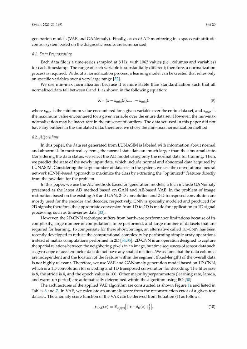
The architectures of the applied VAE algorithm are constructed as shown Figure 1a and listed inTables 6 and 7. In VAE, we calculate an anomaly score from the reconstruction error of a given testdataset. The anomaly score function of the VAE can be derived from Equation (1) as follows:

fVAE(x) = Eq(z|x)

[‖ x− dθ(z) ‖22

], (10)

Sensors 2020, 20, 1991 10 of 20

Sensors 2020, 20, x FOR PEER REVIEW 10 of 21

푓 (푥) = 피 (푧|푥)[∥ 푥 − 푑 (푧) ∥ ] , (10)

Normal cases should have low reconstruction errors, whereas anomalies should have high reconstruction errors.

The detailed network structure and loss functions for optimization are depicted in Figure 1b, Tables 8 and 9, respectively. During the test stage, the model uses encoder loss (퐿 ) given in Equation (2) for scoring the abnormality of the given dataset. Hence, for a test sample 푥, our anomaly score 퐴(푥) is defined with bottleneck features of the input 퐺 (푥) and the encoded features of the generated output 퐸(퐺(푥)) as follows [24]:

퐴(푥) =∥ 퐺 (푥) − 퐸(퐺(푥)) ∥ , (11)

To evaluate the overall anomaly performance, we computed the anomaly score 푆 =푠 ∶ 퐴(푥 ), 푥 ∈ 퐷 for the individual test sample 푥 within the test set 퐷. Then, we applied feature

scaling to obtain the anomaly scores within the probabilistic range of [0, 1].

(a) (b)

Table 6. Encoder part of VAE algorithm

Layer Input → output Operation

Input (n, 1063, 8) *→ (n, 1063, 8) Min / Max Normalization

Hidden (n, 1063, 8) → (n, 531, 4) 1D Convolution, 1D Batch Normalization, Activation Function

(ReLU)

Hidden (n, 531, 4) → (n, 265, 2) 1D Convolution, 1D Batch Normalization, Activation Function

(ReLU)

Hidden (n, 265, 2) → (n, 132, 1) 1D Convolution, 1D Batch Normalization, Activation Function

(ReLU)

Flatten (n, 132, 1) → (n, 132) Flatten

Hidden (n, 132) → (n, 100) Linear, Batch

Normalization, Activation Function (ReLU)

Output Mean Layer (n, 100) → (n, 32) Linear

S.D. Layer (n, 100) → (n, 32) Linear * (batch size, number of channels, kernel size).

Table 7. Decoder part of VAE algorithm

Layer Input → output Operation

Input (n, 32)* → (n, 32) Parameterization

Hidden (n, 32) → (n, 100) Linear, Batch Normalization, Activation

Function (ReLU)

Hidden (n, 100) → (n, 264) Linear, Batch Normalization, Activation

Function (ReLU)

Hidden (n, 264) → (n, 132, 2) Reshape

Hidden (n, 132,2) → (n, 265, 4) 1D Transposed Convolution, 1D Batch

Normalization, Activation Function (ReLU)

Hidden (n, 265, 4) → (n, 531, 5) 1D Transposed Convolution, 1D Batch

Normalization, Activation Function (ReLU)

Output (n, 531, 5) → (n, 1063, 8) 1D Transposed

Convolution

* (batch size, number of channels, kernel size).

Figure 1. Algorithm architectures: (a) anomaly detection (AD) algorithm architecture using variational autoencoder (VAE) structure; (b) AD algorithm architecture using generative adversarial networks AD (GANomaly) structure.

Figure 1. Algorithm architectures: (a) anomaly detection (AD) algorithm architecture using variationalautoencoder (VAE) structure; (b) AD algorithm architecture using generative adversarial networks AD(GANomaly) structure.

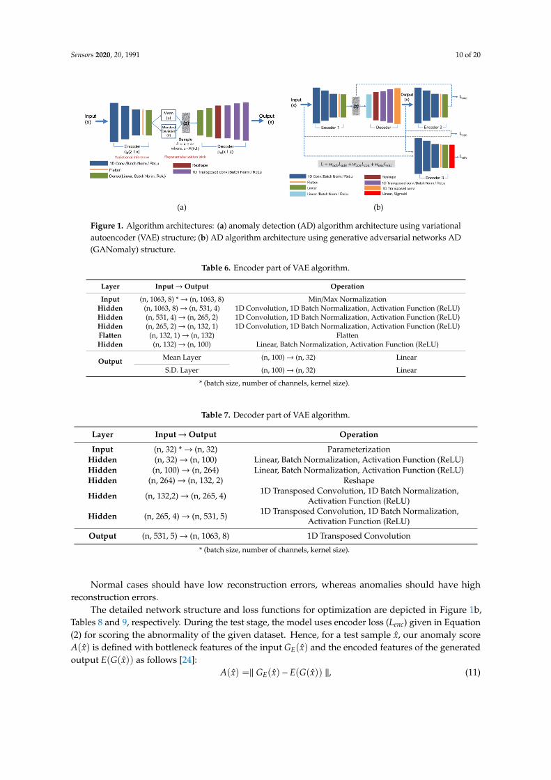
Table 6. Encoder part of VAE algorithm.

Layer Input→ Output Operation

Input (n, 1063, 8) *→ (n, 1063, 8) Min/Max NormalizationHidden (n, 1063, 8)→ (n, 531, 4) 1D Convolution, 1D Batch Normalization, Activation Function (ReLU)Hidden (n, 531, 4)→ (n, 265, 2) 1D Convolution, 1D Batch Normalization, Activation Function (ReLU)Hidden (n, 265, 2)→ (n, 132, 1) 1D Convolution, 1D Batch Normalization, Activation Function (ReLU)Flatten (n, 132, 1)→ (n, 132) FlattenHidden (n, 132)→ (n, 100) Linear, Batch Normalization, Activation Function (ReLU)

Output Mean Layer (n, 100)→ (n, 32) Linear

S.D. Layer (n, 100)→ (n, 32) Linear

* (batch size, number of channels, kernel size).

Table 7. Decoder part of VAE algorithm.

Layer Input→ Output Operation

Input (n, 32) *→ (n, 32) ParameterizationHidden (n, 32)→ (n, 100) Linear, Batch Normalization, Activation Function (ReLU)Hidden (n, 100)→ (n, 264) Linear, Batch Normalization, Activation Function (ReLU)Hidden (n, 264)→ (n, 132, 2) Reshape

Hidden (n, 132,2)→ (n, 265, 4) 1D Transposed Convolution, 1D Batch Normalization,Activation Function (ReLU)

Hidden (n, 265, 4)→ (n, 531, 5) 1D Transposed Convolution, 1D Batch Normalization,Activation Function (ReLU)

Output (n, 531, 5)→ (n, 1063, 8) 1D Transposed Convolution

* (batch size, number of channels, kernel size).

Normal cases should have low reconstruction errors, whereas anomalies should have highreconstruction errors.

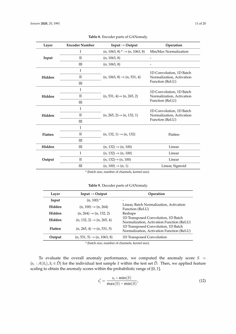
The detailed network structure and loss functions for optimization are depicted in Figure 1b,Tables 8 and 9, respectively. During the test stage, the model uses encoder loss (Lenc) given in Equation(2) for scoring the abnormality of the given dataset. Hence, for a test sample x, our anomaly scoreA(x) is defined with bottleneck features of the input GE(x) and the encoded features of the generatedoutput E(G(x)) as follows [24]:

A(x) =‖ GE(x) − E(G(x)) ‖, (11)

Sensors 2020, 20, 1991 11 of 20

Table 8. Encoder parts of GANomaly.

Layer Encoder Number Input→ Output Operation

Input

I (n, 1063, 8) *→ (n, 1063, 8) Min/Max Normalization

II (n, 1063, 8) -

III (n, 1063, 8) -

Hidden

I

(n, 1063, 8)→ (n, 531, 4)1D Convolution, 1D BatchNormalization, ActivationFunction (ReLU)

II

III

Hidden

I

(n, 531, 4)→ (n, 265, 2)1D Convolution, 1D BatchNormalization, ActivationFunction (ReLU)

II

III

Hidden

I

(n, 265, 2)→ (n, 132, 1)1D Convolution, 1D BatchNormalization, ActivationFunction (ReLU)

II

III

Flatten

I

(n, 132, 1)→ (n, 132) FlattenII

III

Hidden III (n, 132)→ (n, 100) Linear

Output

I (n, 132)→ (n, 100) Linear

II (n, 132)→ (n, 100) Linear

III (n, 100)→ (n, 1) Linear, Sigmoid

* (batch size, number of channels, kernel size).

Table 9. Decoder parts of GANomaly.

Layer Input→ Output Operation

Input (n, 100) * -

Hidden (n, 100)→ (n, 264) Linear, Batch Normalization, ActivationFunction (ReLU)

Hidden (n, 264)→ (n, 132, 2) Reshape

Hidden (n, 132, 2)→ (n, 265, 4) 1D Transposed Convolution, 1D BatchNormalization, Activation Function (ReLU)

Flatten (n, 265, 4)→ (n, 531, 5) 1D Transposed Convolution, 1D BatchNormalization, Activation Function (ReLU)

Output (n, 531, 5)→ (n, 1063, 8) 1D Transposed Convolution

* (batch size, number of channels, kernel size).

To evaluate the overall anomaly performance, we computed the anomaly score S =

{si : A(xi), xi ∈ D} for the individual test sample x within the test set D. Then, we applied featurescaling to obtain the anomaly scores within the probabilistic range of [0, 1].

s′i =si −min(S)

max(S) −min(S), (12)

Sensors 2020, 20, 1991 12 of 20

4.3. Hyperparameter Optimization

Before training a neural network, choosing appropriate hyperparameters is crucial in obtaininga well-generalized neural network for the target task. Traditional ways to select hyperparametersinclude grid search and random search.

Both methods determine ranges of hyperparameter values and train the neural network bychoosing hyperparameters. Although these two methods are sound ways of choosing hyperparameters,the computational complexity increases exponentially with the number of hyperparameters. To alleviatethe computational complexity problem, Snoek et al. [30] proposed a BO. This BO utilizes a GPas a prior for a posterior distribution and samples a performance function whose domain is theset of hyperparameters from the posterior distribution. Finally, by choosing the most successfulhyperparameters, this method can select hyperparameters without an exponentially expensive search.

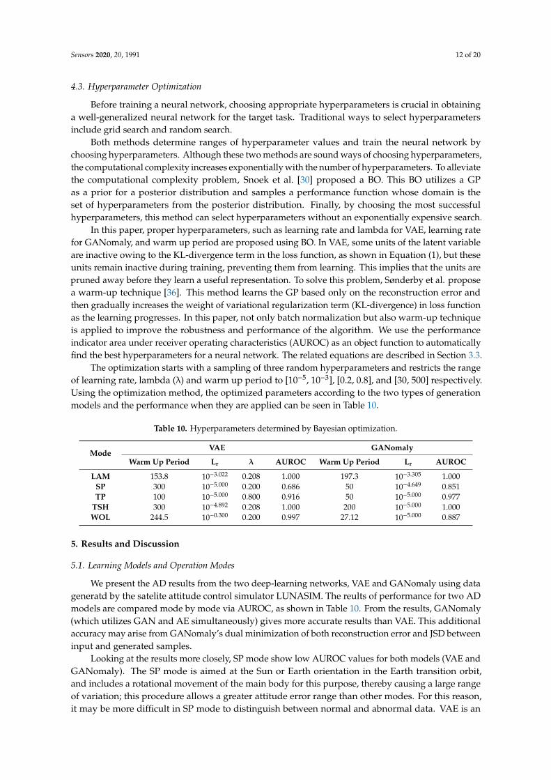
In this paper, proper hyperparameters, such as learning rate and lambda for VAE, learning ratefor GANomaly, and warm up period are proposed using BO. In VAE, some units of the latent variableare inactive owing to the KL-divergence term in the loss function, as shown in Equation (1), but theseunits remain inactive during training, preventing them from learning. This implies that the units arepruned away before they learn a useful representation. To solve this problem, Sønderby et al. proposea warm-up technique [36]. This method learns the GP based only on the reconstruction error andthen gradually increases the weight of variational regularization term (KL-divergence) in loss functionas the learning progresses. In this paper, not only batch normalization but also warm-up techniqueis applied to improve the robustness and performance of the algorithm. We use the performanceindicator area under receiver operating characteristics (AUROC) as an object function to automaticallyfind the best hyperparameters for a neural network. The related equations are described in Section 3.3.

The optimization starts with a sampling of three random hyperparameters and restricts the rangeof learning rate, lambda (λ) and warm up period to [10−5, 10−3], [0.2, 0.8], and [30, 500] respectively.Using the optimization method, the optimized parameters according to the two types of generationmodels and the performance when they are applied can be seen in Table 10.

Table 10. Hyperparameters determined by Bayesian optimization.

ModeVAE GANomaly

Warm Up Period Lr λ AUROC Warm Up Period Lr AUROC

LAM 153.8 10−3.022 0.208 1.000 197.3 10−3.305 1.000SP 300 10−5.000 0.200 0.686 50 10−4.649 0.851TP 100 10−5.000 0.800 0.916 50 10−5.000 0.977

TSH 300 10−4.892 0.208 1.000 200 10−5.000 1.000WOL 244.5 10−0.300 0.200 0.997 27.12 10−5.000 0.887

5. Results and Discussion

5.1. Learning Models and Operation Modes

We present the AD results from the two deep-learning networks, VAE and GANomaly using datageneratd by the satelite attitude control simulator LUNASIM. The reults of performance for two ADmodels are compared mode by mode via AUROC, as shown in Table 10. From the results, GANomaly(which utilizes GAN and AE simultaneously) gives more accurate results than VAE. This additionalaccuracy may arise from GANomaly’s dual minimization of both reconstruction error and JSD betweeninput and generated samples.

Looking at the results more closely, SP mode show low AUROC values for both models (VAE andGANomaly). The SP mode is aimed at the Sun or Earth orientation in the Earth transition orbit,and includes a rotational movement of the main body for this purpose, thereby causing a large rangeof variation; this procedure allows a greater attitude error range than other modes. For this reason,it may be more difficult in SP mode to distinguish between normal and abnormal data. VAE is an

Sensors 2020, 20, 1991 13 of 20

AE variant and probability generative model that regulates latent variables to follow a multivariatenormal distribution. The objective function of VAE consists of two parts: MSE for maximum likelihoodestimation and KL divergence for regularization. Although the KL divergence objective allows VAE tosample more informative latent variables, the sampling process for the reparameterization can causesome noise in the reconstructed output. Therefore, when the normal data and the abnormal data arenot clearly different, the VAE trained only on normal data will generate abnormal samples instead ofnormal ones. Conversely, in the case of GANomaly, there is no such sampling process in the middle ofthe neural network. Additionally, because the GANomaly utilizes AE to reconstruct input data andGAN to match a distribution of generated samples to the target distribution (distribution of normalsamples), GANomaly produces less noisy data than VAE. As a result, GANomaly can discriminateabnormal samples using reconstruction error more effectively than VAE. For this reason, SP and TPmodes show much better results for GANomaly than for VAE and are not suitable for applying VAEtechniques. In other words, normal and abnormal data can be separated easily by VAE in modes likeLAM, TSH and WOL due to the simplicity of the training data set, but such separation cannot beachieved by VAE for SP and TP, which may have some noise in the training data set.

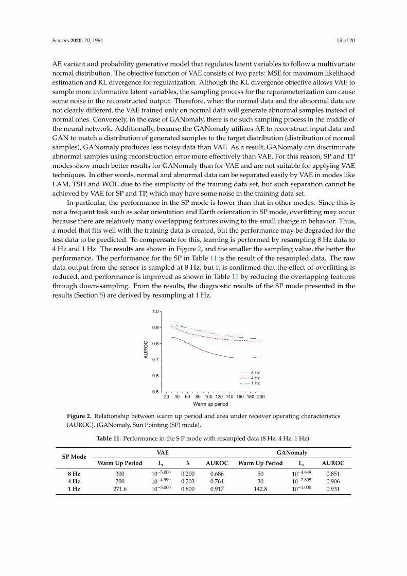
In particular, the performance in the SP mode is lower than that in other modes. Since this isnot a frequent task such as solar orientation and Earth orientation in SP mode, overfitting may occurbecause there are relatively many overlapping features owing to the small change in behavior. Thus,a model that fits well with the training data is created, but the performance may be degraded for thetest data to be predicted. To compensate for this, learning is performed by resampling 8 Hz data to4 Hz and 1 Hz. The results are shown in Figure 2, and the smaller the sampling value, the better theperformance. The performance for the SP in Table 11 is the result of the resampled data. The rawdata output from the sensor is sampled at 8 Hz, but it is confirmed that the effect of overfitting isreduced, and performance is improved as shown in Table 11 by reducing the overlapping featuresthrough down-sampling. From the results, the diagnostic results of the SP mode presented in theresults (Section 5) are derived by resampling at 1 Hz.

Sensors 2020, 20, x FOR PEER REVIEW 13 of 21

Hz and 1 Hz. The results are shown in Figure 2, and the smaller the sampling value, the better the performance. The performance for the SP in Table 11 is the result of the resampled data. The raw data output from the sensor is sampled at 8 Hz, but it is confirmed that the effect of overfitting is reduced, and performance is improved as shown in Table 11 by reducing the overlapping features through down-sampling. From the results, the diagnostic results of the SP mode presented in the results (chapter 5) are derived by resampling at 1 Hz.

Figure 2. Relationship between warm up period and area under receiver operating characteristics (AUROC), (GANomaly, Sun Pointing (SP) mode).

Table 11. Performance in the S P mode with resampled data (8 Hz, 4 Hz, 1 Hz).

SP Mode VAE GANomaly

Warm up period Lr λ AUROC Warm up period Lr AUROC

8 Hz 300 10−5.000 0.200 0.686 50 10−4.649 0.851

4 Hz 200 10−4.999 0.203 0.764 30 10−2.805 0.906

1 Hz 271.6 10−5.000 0.800 0.917 142.8 10−1.000 0.931

5.2. Assistive Tools for AD

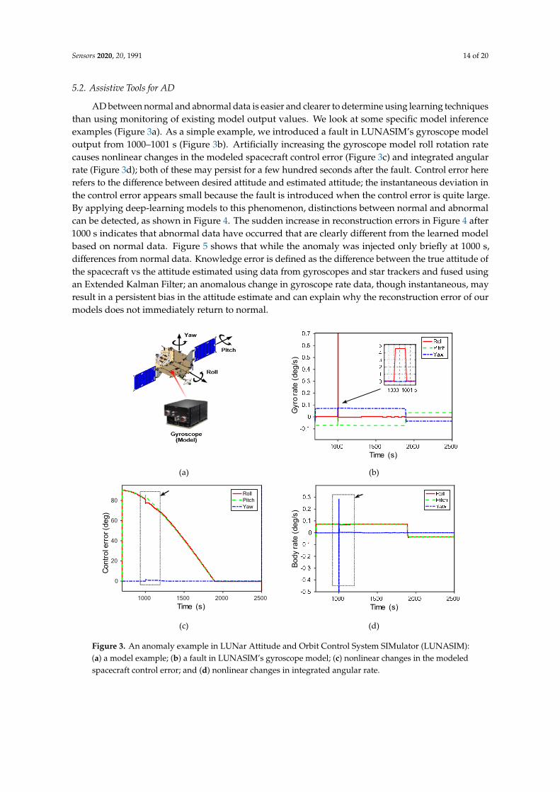
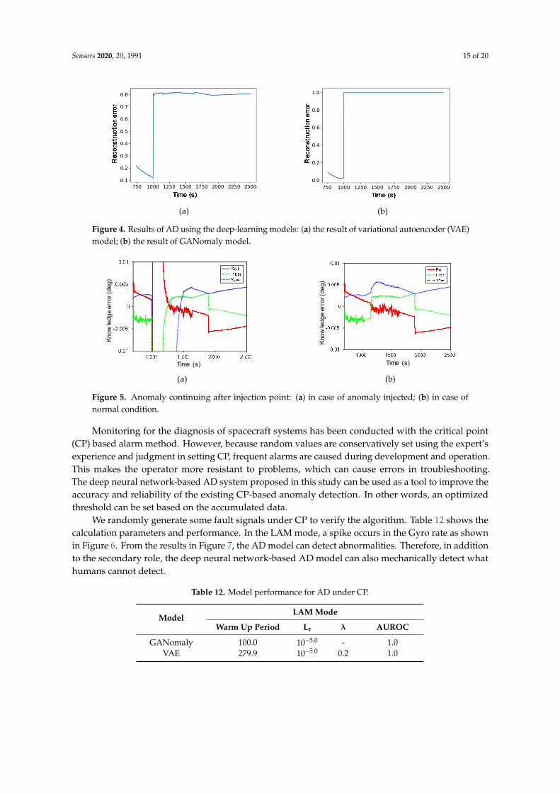
AD between normal and abnormal data is easier and clearer to determine using learning techniques than using monitoring of existing model output values. We look at some specific model inference examples (Figure 3a). As a simple example, we introduced a fault in LUNASIM’s gyroscope model output from 1000–1001 s (Figure 3b). Artificially increasing the gyroscope model roll rotation rate causes nonlinear changes in the modeled spacecraft control error (Figure 3c) and integrated angular rate (Figure 3d); both of these may persist for a few hundred seconds after the fault. Control error here refers to the difference between desired attitude and estimated attitude; the instantaneous deviation in the control error appears small because the fault is introduced when the control error is quite large. By applying deep-learning models to this phenomenon, distinctions between normal and abnormal can be detected, as shown in Figure 4. The sudden increase in reconstruction errors in Figure 4 after 1000 s indicates that abnormal data have occurred that are clearly different from the learned model based on normal data. Figure 5 shows that while the anomaly was injected only briefly at 1000 s, differences from normal data. Knowledge error is defined as the difference between the true attitude of the spacecraft vs the attitude estimated using data from gyroscopes and star trackers and fused using an Extended Kalman Filter; an anomalous change in gyroscope rate data, though instantaneous, may result in a persistent bias in the attitude estimate and can explain why the reconstruction error of our models does not immediately return to normal.

20 40 60 80 100 120 140 160 180 2000.5

0.6

0.7

0.8

0.9

1.0

AUR

OC

Warm up period

8 Hz 4 Hz 1 Hz

Figure 2. Relationship between warm up period and area under receiver operating characteristics(AUROC), (GANomaly, Sun Pointing (SP) mode).

Table 11. Performance in the S P mode with resampled data (8 Hz, 4 Hz, 1 Hz).

SP ModeVAE GANomaly

Warm Up Period Lr λ AUROC Warm Up Period Lr AUROC

8 Hz 300 10−5.000 0.200 0.686 50 10−4.649 0.8514 Hz 200 10−4.999 0.203 0.764 30 10−2.805 0.9061 Hz 271.6 10−5.000 0.800 0.917 142.8 10−1.000 0.931

Sensors 2020, 20, 1991 14 of 20

5.2. Assistive Tools for AD

AD between normal and abnormal data is easier and clearer to determine using learning techniquesthan using monitoring of existing model output values. We look at some specific model inferenceexamples (Figure 3a). As a simple example, we introduced a fault in LUNASIM’s gyroscope modeloutput from 1000–1001 s (Figure 3b). Artificially increasing the gyroscope model roll rotation ratecauses nonlinear changes in the modeled spacecraft control error (Figure 3c) and integrated angularrate (Figure 3d); both of these may persist for a few hundred seconds after the fault. Control error hererefers to the difference between desired attitude and estimated attitude; the instantaneous deviation inthe control error appears small because the fault is introduced when the control error is quite large.By applying deep-learning models to this phenomenon, distinctions between normal and abnormalcan be detected, as shown in Figure 4. The sudden increase in reconstruction errors in Figure 4 after1000 s indicates that abnormal data have occurred that are clearly different from the learned modelbased on normal data. Figure 5 shows that while the anomaly was injected only briefly at 1000 s,differences from normal data. Knowledge error is defined as the difference between the true attitude ofthe spacecraft vs the attitude estimated using data from gyroscopes and star trackers and fused usingan Extended Kalman Filter; an anomalous change in gyroscope rate data, though instantaneous, mayresult in a persistent bias in the attitude estimate and can explain why the reconstruction error of ourmodels does not immediately return to normal.Sensors 2020, 20, x FOR PEER REVIEW 14 of 21

(a) (b)

(c) (d)

Figure 3. An anomaly example in LUNar Attitude and Orbit Control System SIMulator (LUNASIM): (a) a model example; (b) a fault in LUNASIM’s gyroscope model; (c) nonlinear changes in the modeled spacecraft control error; and (d) nonlinear changes in integrated angular rate.

(a)

(b)

Figure 4. Results of AD using the deep-learning models: (a) the result of variational autoencoder (VAE) model; (b) the result of GANomaly model.

Time (s)

Gyr

o ra

te (d

eg/s

)

1000 1500 2000 2500Time(s)

0

20

40

60

80RollPitchYaw

Time (s)

Cont

rol e

rror

(deg

)

Time (s)

Body

rate

(deg

/s)

Figure 3. An anomaly example in LUNar Attitude and Orbit Control System SIMulator (LUNASIM):(a) a model example; (b) a fault in LUNASIM’s gyroscope model; (c) nonlinear changes in the modeledspacecraft control error; and (d) nonlinear changes in integrated angular rate.

Sensors 2020, 20, 1991 15 of 20

Sensors 2020, 20, x FOR PEER REVIEW 14 of 21

(a) (b)

(c) (d)

Figure 3. An anomaly example in LUNar Attitude and Orbit Control System SIMulator (LUNASIM): (a) a model example; (b) a fault in LUNASIM’s gyroscope model; (c) nonlinear changes in the modeled spacecraft control error; and (d) nonlinear changes in integrated angular rate.

(a)

(b)

Figure 4. Results of AD using the deep-learning models: (a) the result of variational autoencoder (VAE) model; (b) the result of GANomaly model.

Time (s)

Gyr

o ra

te (d

eg/s

)

1000 1500 2000 2500Time(s)

0

20

40

60

80RollPitchYaw

Time (s)

Cont

rol e

rror

(deg

)

Time (s)

Body

rate

(deg

/s)

Figure 4. Results of AD using the deep-learning models: (a) the result of variational autoencoder (VAE)model; (b) the result of GANomaly model.

Sensors 2020, 20, x FOR PEER REVIEW 15 of 21

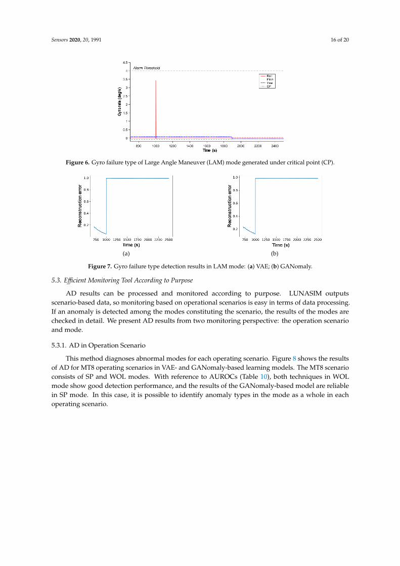
Monitoring for the diagnosis of spacecraft systems has been conducted with the critical point (CP) based alarm method. However, because random values are conservatively set using the expert’s experience and judgment in setting CP, frequent alarms are caused during development and operation. This makes the operator more resistant to problems, which can cause errors in troubleshooting. The deep neural network-based AD system proposed in this study can be used as a tool to improve the accuracy and reliability of the existing CP-based anomaly detection. In other words, an optimized threshold can be set based on the accumulated data.

We randomly generate some fault signals under CP to verify the algorithm. Table 12 shows the calculation parameters and performance. In the LAM mode, a spike occurs in the Gyro rate as shown in Figure 6. From the results in Figure 7, the AD model can detect abnormalities. Therefore, in addition to the secondary role, the deep neural network-based AD model can also mechanically detect what humans cannot detect.

Table 12. Model performance for AD under CP.

Model LAM mode

Warm up period Lr λ AUROC GANomaly 100.0 10−5.0 - 1.0

VAE 279.9 10−5.0 0.2 1.0

Figure 6. Gyro failure type of Large Angle Maneuver (LAM) mode generated under critical

point (CP).

(a)

(b)

Figure 5. Anomaly continuing after injection point: (a) in case of anomaly injected; (b) in case of normal condition.

Time (s)

Know

ledg

e er

ror (

deg)

Kno

wle

dge

Err

or(d

eg)

Know

ledg

e er

ror (

deg)

Time (s)

Figure 5. Anomaly continuing after injection point: (a) in case of anomaly injected; (b) in case ofnormal condition.

Monitoring for the diagnosis of spacecraft systems has been conducted with the critical point(CP) based alarm method. However, because random values are conservatively set using the expert’sexperience and judgment in setting CP, frequent alarms are caused during development and operation.This makes the operator more resistant to problems, which can cause errors in troubleshooting.The deep neural network-based AD system proposed in this study can be used as a tool to improve theaccuracy and reliability of the existing CP-based anomaly detection. In other words, an optimizedthreshold can be set based on the accumulated data.

We randomly generate some fault signals under CP to verify the algorithm. Table 12 shows thecalculation parameters and performance. In the LAM mode, a spike occurs in the Gyro rate as shownin Figure 6. From the results in Figure 7, the AD model can detect abnormalities. Therefore, in additionto the secondary role, the deep neural network-based AD model can also mechanically detect whathumans cannot detect.

Table 12. Model performance for AD under CP.

ModelLAM Mode

Warm Up Period Lr λ AUROC

GANomaly 100.0 10−5.0 - 1.0VAE 279.9 10−5.0 0.2 1.0

Sensors 2020, 20, 1991 16 of 20

Sensors 2020, 20, x FOR PEER REVIEW 15 of 21

Monitoring for the diagnosis of spacecraft systems has been conducted with the critical point (CP) based alarm method. However, because random values are conservatively set using the expert’s experience and judgment in setting CP, frequent alarms are caused during development and operation. This makes the operator more resistant to problems, which can cause errors in troubleshooting. The deep neural network-based AD system proposed in this study can be used as a tool to improve the accuracy and reliability of the existing CP-based anomaly detection. In other words, an optimized threshold can be set based on the accumulated data.

We randomly generate some fault signals under CP to verify the algorithm. Table 12 shows the calculation parameters and performance. In the LAM mode, a spike occurs in the Gyro rate as shown in Figure 6. From the results in Figure 7, the AD model can detect abnormalities. Therefore, in addition to the secondary role, the deep neural network-based AD model can also mechanically detect what humans cannot detect.

Table 12. Model performance for AD under CP.

Model LAM mode

Warm up period Lr λ AUROC GANomaly 100.0 10−5.0 - 1.0

VAE 279.9 10−5.0 0.2 1.0

Figure 6. Gyro failure type of Large Angle Maneuver (LAM) mode generated under critical

point (CP).

(a)

(b)

Figure 5. Anomaly continuing after injection point: (a) in case of anomaly injected; (b) in case of normal condition.

Time (s)

Know

ledg

e er

ror (

deg)

Kno

wle

dge

Err

or(d

eg)

Know

ledg

e er

ror (

deg)

Time (s)

Figure 6. Gyro failure type of Large Angle Maneuver (LAM) mode generated under critical point (CP).Sensors 2020, 20, x FOR PEER REVIEW 16 of 21

(a) (b)

Figure 7. Gyro failure type detection results in LAM mode: (a) VAE; (b) GANomaly.

5.3. Efficient Monitoring Tool According to Purpose

AD results can be processed and monitored according to purpose. LUNASIM outputs scenario-based data, so monitoring based on operational scenarios is easy in terms of data processing. If an anomaly is detected among the modes constituting the scenario, the results of the modes are checked in detail. We present AD results from two monitoring perspective: the operation scenario and mode.

5.3.1. AD In Operation Scenario

This method diagnoses abnormal modes for each operating scenario. Figure 8 shows the results of AD for MT8 operating scenarios in VAE- and GANomaly-based learning models. The MT8 scenario consists of SP and WOL modes. With reference to AUROCs (Table 10), both techniques in WOL mode show good detection performance, and the results of the GANomaly-based model are reliable in SP mode. In this case, it is possible to identify anomaly types in the mode as a whole in each operating scenario.

(a)

(b)

Figure 8. Failure types of each mode in MT8 scenario: (a) the result of GANomaly model; (b) the result of VAE model.

5.3.2. AD In Operation Mode

Figure 7. Gyro failure type detection results in LAM mode: (a) VAE; (b) GANomaly.

5.3. Efficient Monitoring Tool According to Purpose

AD results can be processed and monitored according to purpose. LUNASIM outputsscenario-based data, so monitoring based on operational scenarios is easy in terms of data processing.If an anomaly is detected among the modes constituting the scenario, the results of the modes arechecked in detail. We present AD results from two monitoring perspective: the operation scenarioand mode.

5.3.1. AD in Operation Scenario

This method diagnoses abnormal modes for each operating scenario. Figure 8 shows the resultsof AD for MT8 operating scenarios in VAE- and GANomaly-based learning models. The MT8 scenarioconsists of SP and WOL modes. With reference to AUROCs (Table 10), both techniques in WOLmode show good detection performance, and the results of the GANomaly-based model are reliablein SP mode. In this case, it is possible to identify anomaly types in the mode as a whole in eachoperating scenario.

Sensors 2020, 20, 1991 17 of 20

Sensors 2020, 20, x FOR PEER REVIEW 16 of 21

(a) (b)

Figure 7. Gyro failure type detection results in LAM mode: (a) VAE; (b) GANomaly.

5.3. Efficient Monitoring Tool According to Purpose

AD results can be processed and monitored according to purpose. LUNASIM outputs scenario-based data, so monitoring based on operational scenarios is easy in terms of data processing. If an anomaly is detected among the modes constituting the scenario, the results of the modes are checked in detail. We present AD results from two monitoring perspective: the operation scenario and mode.

5.3.1. AD In Operation Scenario

This method diagnoses abnormal modes for each operating scenario. Figure 8 shows the results of AD for MT8 operating scenarios in VAE- and GANomaly-based learning models. The MT8 scenario consists of SP and WOL modes. With reference to AUROCs (Table 10), both techniques in WOL mode show good detection performance, and the results of the GANomaly-based model are reliable in SP mode. In this case, it is possible to identify anomaly types in the mode as a whole in each operating scenario.

(a)

(b)

Figure 8. Failure types of each mode in MT8 scenario: (a) the result of GANomaly model; (b) the result of VAE model.

5.3.2. AD In Operation Mode

Figure 8. Failure types of each mode in MT8 scenario: (a) the result of GANomaly model; (b) the resultof VAE model.

5.3.2. AD in Operation Mode

If an anomaly occurs during spacecraft operation, the anomaly can be detected in each operatingmode. Figure 9 shows the failure types in the LAM operating mode. A failure detected with acontinuous reconstruction error of 0.996 or higher indicates an RWA failure, and the peak near 1000and 2000 s is caused by an RWA wheel speed spike. Also, a failure persisting from around 1500 to2000 s, indicates a gyroscope rate spike. The pattern of each type of failure is distinct, so it is easy todistinguish among failures given knowledge of typical failure types.

Sensors 2020, 20, x FOR PEER REVIEW 17 of 21

If an anomaly occurs during spacecraft operation, the anomaly can be detected in each operating mode. Figure 9 shows the failure types in the LAM operating mode. A failure detected with a continuous reconstruction error of 0.996 or higher indicates an RWA failure, and the peak near 1000 and 2000 s is caused by an RWA wheel speed spike. Also, a failure persisting from around 1500 to 2000 s, indicates a gyroscope rate spike. The pattern of each type of failure is distinct, so it is easy to distinguish among failures given knowledge of typical failure types.

(a)

(b)

Figure 9. Anomaly types in LAM mode: (a) the result of GANomaly model; (b) the result of VAE model.

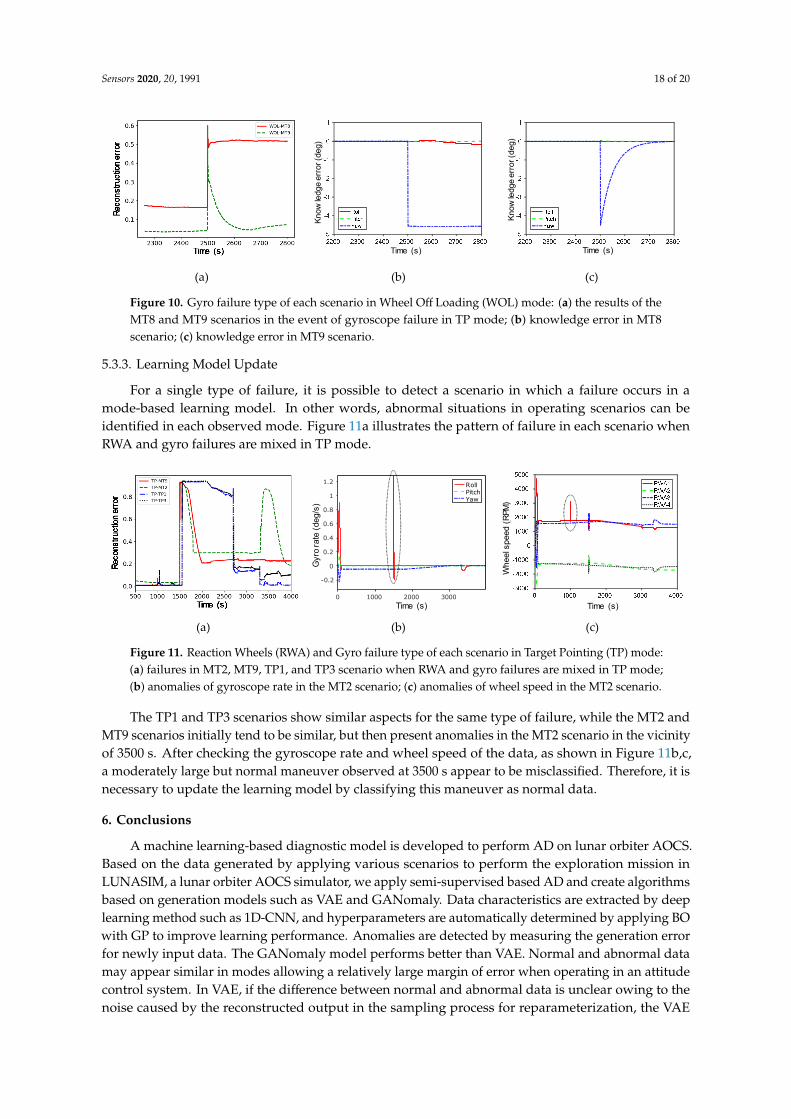
Figure 10a shows the observed results in the MT8 and MT9 scenarios in the event of gyroscope failure in TP mode. In both scenarios, failure patterns tended to be similar, followed by failures around 2500 s. Reconstruction errors are consistently high in the MT8 scenario, but not so in MT9. In this regard, the knowledge error values of gyroscopes presented in Figure 10b,c can be analyzed to determine what caused them. In the MT8 scenario, the yaw axis knowledge error was continuously high after abnormal behavior at 2500 s, and in the MT9 scenario, the value increased at the anomalous behavior but converged afterwards. As shown, even if the failure type is the same, there may be a difference in the failure occurrence pattern for each scenario. By monitoring the diagnosis result, it is possible to identify the cause of the failure in the system. If the cause is normal behavior, it is used as normal data to retrain the learning model.

5.3.3. Learning Model Update

For a single type of failure, it is possible to detect a scenario in which a failure occurs in a mode-based learning model. In other words, abnormal situations in operating scenarios can be identified

(a)

(b)

(c)

Figure 10. Gyro failure type of each scenario in Wheel Off Loading (WOL) mode: (a) the results of the MT8 and MT9 scenarios in the event of gyroscope failure in TP mode; (b) knowledge error in MT8 scenario; (c) knowledge error in MT9 scenario.

Kno

wle

dge

Err

or(d

eg)

Know

ledg

e er

ror (

deg)

Time (s)

Know

ledg

e er

ror (

deg)

Time (s)

Figure 9. Anomaly types in LAM mode: (a) the result of GANomaly model; (b) the result of VAE model.

Figure 10a shows the observed results in the MT8 and MT9 scenarios in the event of gyroscopefailure in TP mode. In both scenarios, failure patterns tended to be similar, followed by failuresaround 2500 s. Reconstruction errors are consistently high in the MT8 scenario, but not so in MT9.In this regard, the knowledge error values of gyroscopes presented in Figure 10b,c can be analyzed todetermine what caused them. In the MT8 scenario, the yaw axis knowledge error was continuouslyhigh after abnormal behavior at 2500 s, and in the MT9 scenario, the value increased at the anomalousbehavior but converged afterwards. As shown, even if the failure type is the same, there may be adifference in the failure occurrence pattern for each scenario. By monitoring the diagnosis result, it ispossible to identify the cause of the failure in the system. If the cause is normal behavior, it is used asnormal data to retrain the learning model.

Sensors 2020, 20, 1991 18 of 20

Sensors 2020, 20, x FOR PEER REVIEW 17 of 21

If an anomaly occurs during spacecraft operation, the anomaly can be detected in each operating mode. Figure 9 shows the failure types in the LAM operating mode. A failure detected with a continuous reconstruction error of 0.996 or higher indicates an RWA failure, and the peak near 1000 and 2000 s is caused by an RWA wheel speed spike. Also, a failure persisting from around 1500 to 2000 s, indicates a gyroscope rate spike. The pattern of each type of failure is distinct, so it is easy to distinguish among failures given knowledge of typical failure types.

(a)

(b)

Figure 9. Anomaly types in LAM mode: (a) the result of GANomaly model; (b) the result of VAE model.

Figure 10a shows the observed results in the MT8 and MT9 scenarios in the event of gyroscope failure in TP mode. In both scenarios, failure patterns tended to be similar, followed by failures around 2500 s. Reconstruction errors are consistently high in the MT8 scenario, but not so in MT9. In this regard, the knowledge error values of gyroscopes presented in Figure 10b,c can be analyzed to determine what caused them. In the MT8 scenario, the yaw axis knowledge error was continuously high after abnormal behavior at 2500 s, and in the MT9 scenario, the value increased at the anomalous behavior but converged afterwards. As shown, even if the failure type is the same, there may be a difference in the failure occurrence pattern for each scenario. By monitoring the diagnosis result, it is possible to identify the cause of the failure in the system. If the cause is normal behavior, it is used as normal data to retrain the learning model.

5.3.3. Learning Model Update

For a single type of failure, it is possible to detect a scenario in which a failure occurs in a mode-based learning model. In other words, abnormal situations in operating scenarios can be identified

(a)

(b)

(c)

Figure 10. Gyro failure type of each scenario in Wheel Off Loading (WOL) mode: (a) the results of the MT8 and MT9 scenarios in the event of gyroscope failure in TP mode; (b) knowledge error in MT8 scenario; (c) knowledge error in MT9 scenario.

Kno

wle

dge

Err

or(d

eg)

Know

ledg

e er

ror (

deg)

Time (s)

Know

ledg

e er

ror (

deg)

Time (s)

Figure 10. Gyro failure type of each scenario in Wheel Off Loading (WOL) mode: (a) the results of theMT8 and MT9 scenarios in the event of gyroscope failure in TP mode; (b) knowledge error in MT8scenario; (c) knowledge error in MT9 scenario.

5.3.3. Learning Model Update

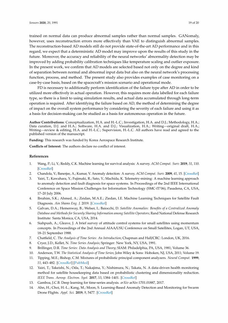
For a single type of failure, it is possible to detect a scenario in which a failure occurs in amode-based learning model. In other words, abnormal situations in operating scenarios can beidentified in each observed mode. Figure 11a illustrates the pattern of failure in each scenario whenRWA and gyro failures are mixed in TP mode.

Sensors 2020, 20, x FOR PEER REVIEW 18 of 21

in each observed mode. Figure 11a illustrates the pattern of failure in each scenario when RWA and gyro failures are mixed in TP mode.

The TP1 and TP3 scenarios show similar aspects for the same type of failure, while the MT2 and MT9 scenarios initially tend to be similar, but then present anomalies in the MT2 scenario in the vicinity of 3500 s. After checking the gyroscope rate and wheel speed of the data, as shown in Figure 11b,c, a moderately large but normal maneuver observed at 3500 s appear to be misclassified. Therefore, it is necessary to update the learning model by classifying this maneuver as normal data.

(a) (b) (c)

Figure 11. Reaction Wheels (RWA) and Gyro failure type of each scenario in Target Pointing (TP) mode: (a) failures in MT2, MT9, TP1, and TP3 scenario when RWA and gyro failures are mixed in TP mode; (b) anomalies of gyroscope rate in the MT2 scenario; (c) anomalies of wheel speed in the MT2 scenario.

0 1000 2000 3000T ime(s )

-0.2

0

0.2

0.4

0.6

0.8

1

1.2

GyroRate(degs)

RollPitchYaw

Time (s)

Gyr

o ra

te (d

eg/s

)

Time (s)

Whe

elsp

eed

(RPM

)

Figure 11. Reaction Wheels (RWA) and Gyro failure type of each scenario in Target Pointing (TP) mode:(a) failures in MT2, MT9, TP1, and TP3 scenario when RWA and gyro failures are mixed in TP mode;(b) anomalies of gyroscope rate in the MT2 scenario; (c) anomalies of wheel speed in the MT2 scenario.

The TP1 and TP3 scenarios show similar aspects for the same type of failure, while the MT2 andMT9 scenarios initially tend to be similar, but then present anomalies in the MT2 scenario in the vicinityof 3500 s. After checking the gyroscope rate and wheel speed of the data, as shown in Figure 11b,c,a moderately large but normal maneuver observed at 3500 s appear to be misclassified. Therefore, it isnecessary to update the learning model by classifying this maneuver as normal data.

6. Conclusions

A machine learning-based diagnostic model is developed to perform AD on lunar orbiter AOCS.Based on the data generated by applying various scenarios to perform the exploration mission inLUNASIM, a lunar orbiter AOCS simulator, we apply semi-supervised based AD and create algorithmsbased on generation models such as VAE and GANomaly. Data characteristics are extracted by deeplearning method such as 1D-CNN, and hyperparameters are automatically determined by applying BOwith GP to improve learning performance. Anomalies are detected by measuring the generation errorfor newly input data. The GANomaly model performs better than VAE. Normal and abnormal datamay appear similar in modes allowing a relatively large margin of error when operating in an attitudecontrol system. In VAE, if the difference between normal and abnormal data is unclear owing to thenoise caused by the reconstructed output in the sampling process for reparameterization, the VAE

Sensors 2020, 20, 1991 19 of 20

trained on normal data can produce abnormal samples rather than normal samples. GANomaly,however, uses reconstruction errors more effectively than VAE to distinguish abnormal samples.The reconstruction-based AD models still do not provide state-of-the-art AD performance and in thisregard, we expect that a deterministic AD model may improve upon the results of this study in thefuture. Moreover, the accuracy and reliability of the neural networks’ abnormality detection may beimproved by adding probability calibration techniques like temperature scaling and outlier exposure.In the present work, we confirm that AD models are selected based not only on the degree and kindof separation between normal and abnormal input data but also on the neural network’s processingfunction, process, and method. The present study also provides examples of case monitoring on acase-by-case basis, based on the spacecraft’s mission scenario and operational mode.

FD is necessary to additionally perform identification of the failure type after AD in order to beutilized more effectively in actual operation. However, this requires more data labelled for each failuretype, so there is a limit to using simulation results, and actual data accumulated through long-termoperation is required. After identifying the failure based on AD, the method of determining the degreeof impact on the overall system performance by considering the severity of each failure and using it asa basis for decision-making can be studied as a basis for autonomous operation in the future.

Author Contributions: Conceptualization, H.A. and H.-L.C.; Investigation, H.A. and D.J.; Methodology, H.A.;Data curation, D.J. and H.A.; Software, H.A. and D.J.; Visualization, H.A.; Writing—original draft, H.A.;Writing—review & editing, H.A. and H.-L.C.; Supervision, H.-L.C. All authors have read and agreed to thepublished version of the manuscript.

Funding: This research was funded by Korea Aerospace Research Institute.

Conflicts of Interest: The authors declare no conflict of interest.

References

1. Wang, P.; Li, Y.; Reddy, C.K. Machine learning for survival analysis: A survey. ACM Comput. Surv. 2019, 51, 110.[CrossRef]

2. Chandola, V.; Banerjee, A.; Kumar, V. Anomaly detection: A survey. ACM Comput. Surv. 2009, 41, 15. [CrossRef]3. Yairi, T.; Kawahara, Y.; Fujimaki, R.; Sato, Y.; Machida, K. Telemetry-mining: A machine learning approach

to anomaly detection and fault diagnosis for space systems. In Proceedings of the 2nd IEEE InternationalConference on Space Mission Challenges for Information Technology (SMC-IT’06), Pasadena, CA, USA,17–20 July 2006.

4. Ibrahim, S.K.; Ahmed, A.; Zeidan, M.A.E.; Ziedan, I.E. Machine Learning Techniques for Satellite FaultDiagnosis. Ain Shams Eng. J. 2019. [CrossRef]

5. Galvan, D.A.; Hemenway, B.; Welser, I.; Baiocchi, D. Satellite Anomalies: Benefits of a Centralized AnomalyDatabase and Methods for Securely Sharing Information among Satellite Operators; Rand National Defense ResearchInstitute: Santa Monica, CA, USA, 2014.

6. Siahpush, A.; Gleave, J. A brief survey of attitude control systems for small satellites using momentumconcepts. In Proceedings of the 2nd Annual AIAA/USU Conference on Small Satellites, Logan, UT, USA,18–21 September 1988.

7. Chatfield, C. The Analysis of Time Series: An Introduction; Chapman and Hall/CRC: London, UK, 2016.8. Cryer, J.D.; Kellet, N. Time Series Analysis; Springer: New York, NY, USA, 1991.9. Brillinger, D.R. Time Series: Data Analysis and Theory; SIAM: Philadelphia, PA, USA, 1981; Volume 36.10. Anderson, T.W. The Statistical Analysis of Time Series; John Wiley & Sons: Hoboken, NJ, USA, 2011; Volume 19.11. Tipping, M.E.; Bishop, C.M. Mixtures of probabilistic principal component analyzers. Neural Comput. 1999,

11, 443–482. [CrossRef] [PubMed]12. Yairi, T.; Takeishi, N.; Oda, T.; Nakajima, Y.; Nishimura, N.; Takata, N. A data-driven health monitoring

method for satellite housekeeping data based on probabilistic clustering and dimensionality reduction.IEEE Trans. Aerosp. Electron. Syst. 2017, 53, 1384–1401. [CrossRef]

13. Gamboa, J.C.B. Deep learning for time-series analysis. arXiv arXiv:1701.01887, 2017.14. Ahn, H.; Choi, H.-L.; Kang, M.; Moon, S. Learning-Based Anomaly Detection and Monitoring for Swarm

Drone Flights. Appl. Sci. 2019, 9, 5477. [CrossRef]

Sensors 2020, 20, 1991 20 of 20

15. Längkvist, M. Modeling Time-Series with Deep Networks; Örebro University: Örebro, Sweden, 2014.16. OMeara, C.; Schlag, L.; Wickler, M. Applications of Deep Learning Neural Networks to Satellite Telemetry

Monitoring. In Proceedings of the 2018 SpaceOps Conference, Marseille, France, 28 May–1 June 2018; p. 2558.17. Wei, W.; Wu, H.; Ma, H. An autoencoder and LSTM-based traffic flow prediction method. Sensors 2019,

19, 2946. [CrossRef] [PubMed]18. Park, P.; Marco, P.D.; Shin, H.; Bang, J. Fault Detection and Diagnosis Using Combined Autoencoder and

Long Short-Term Memory Network. Sensors 2019, 19, 4612. [CrossRef] [PubMed]19. Liu, X.; Zhou, Q.; Zhao, J.; Shen, H.; Xiong, X. Fault Diagnosis of Rotating Machinery under Noisy

Environment Conditions Based on a 1-D Convolutional Autoencoder and 1-D Convolutional NeuralNetwork. Sensors 2019, 19, 972. [CrossRef] [PubMed]

20. Chen, K.; Mao, Z.; Zhao, H.; Jiang, Z.; Zhang, J. A Variational Stacked Autoencoder with Harmony SearchOptimizer for Valve Train Fault Diagnosis of Diesel Engine. Sensors 2020, 20, 223. [CrossRef] [PubMed]

21. Jung, D.; Kwon, J.W.; Baek, K.; Ahn, H.W. Attitude Control Simulator for the Korea Pathfinder Lunar Orbiter.In Asia-Pacific International Symposium on Aerospace Technology; Springer: Singapore, 2018; pp. 2521–2532.

22. Jung, D.; Kwon, J.W.; Seo, H.H.; Yim, J.R. New Concepts for the Korea Pathfinder Lunar Orbiter AttitudeControl System Simulator. In Proceedings of the 2017 Asia-Pacific International Symposium on AerospaceTechnology, Seoul, Korea, 16–18 October 2017; pp. 637–638.

23. Kingma, D.P.; Welling, M. Auto-encoding variational bayes. arXiv arXiv:1312.6114, 2013.24. Akcay, S.; Atapour-Abarghouei, A.; Breckon, T.P. Ganomaly: Semi-supervised anomaly detection via

adversarial training. In Asian Conference on Computer Vision; Springer: Cham, Switzerland, 2018; pp. 622–637.25. Bourlard, H.; Kamp, Y. Auto-association by multilayer perceptrons and singular value decomposition.

Biol. Cybern. 1988, 59, 291–294. [CrossRef] [PubMed]26. Škvára, V.; Pevný, T.; Šmídl, V. Are generative deep models for novelty detection truly better? arXiv

arXiv:1807.05027, 2018.27. Kullback, S.; Leibler, R.A. On information and sufficiency. Ann. Math. Stat. 1951, 22, 79–86. [CrossRef]28. Goodfellow, I.; Pouget-Abadie, J.; Mirza, M.; Xu, B.; Warde-Farley, D.; Ozair, S.; Courville, A.; Bengio, Y.

Generative adversarial nets. In Proceedings of the Neural Information Processing Systems, Montreal, QC,Canada, 8–13 December 2014; pp. 2672–2680.

29. Schlegl, T.; Seeböck, P.; Waldstein, S.M.; Schmidt-Erfurth, U.; Langs, G. Unsupervised anomaly detection withgenerative adversarial networks to guide marker discovery. In Proceedings of the International Conferenceon Information Processing in Medical Imaging, University in Boone, Boone, NC, USA, 25–30 June 2017;pp. 146–157.

30. Snoek, J.; Larochelle, H.; Adams, R.P. Practical bayesian optimization of machine learning algorithms.In Proceedings of the Neural Information Processing Systems, Lake Tahoe, NV, USA, 3–8 December 2012;pp. 2951–2959.

31. Pedregosa, F.; Varoquaux, G.; Gramfort, A.; Michel, V.; Thirion, B.; Grisel, O.; Blondel, M.; Prettenhofer, P.;Weiss, R.; Dubourg, V. Scikit-learn: Machine learning in Python. J. Mach. Learn. Res. 2011, 12, 2825–2830.

32. Sola, J.; Sevilla, J. Importance of input data normalization for the application of neural networks to complexindustrial problems. IEEE Trans. Nucl. Sci. 1997, 44, 1464–1468. [CrossRef]

33. Kiranyaz, S.; Avci, O.; Abdeljaber, O.; Ince, T.; Gabbouj, M.; Inman, D.J. 1D Convolutional Neural Networksand Applications: A Survey. arXiv arXiv:1905.03554, 2019.

34. Abdeljaber, O.; Avci, O.; Kiranyaz, S.; Gabbouj, M.; Inman, D.J. Real-time vibration-based structural damagedetection using one-dimensional convolutional neural networks. J. Sound Vib. 2017, 388, 154–170. [CrossRef]

35. Ince, T.; Kiranyaz, S.; Eren, L.; Askar, M.; Gabbouj, M. Real-time motor fault detection by 1-D convolutionalneural networks. IEEE Trans. Ind. Electron. 2016, 63, 7067–7075. [CrossRef]

36. Sønderby, C.K.; Raiko, T.; Maaløe, L.; Sønderby, S.K.; Winther, O. How to train deep variational autoencodersand probabilistic ladder networks. In Proceedings of the 33rd International Conference on Machine Learning(ICML 2016), New York, NY, USA, 19–24 June 2016.

© 2020 by the authors. Licensee MDPI, Basel, Switzerland. This article is an open accessarticle distributed under the terms and conditions of the Creative Commons Attribution(CC BY) license (http://creativecommons.org/licenses/by/4.0/).