Spacecraft Formation Flying Control using Mean Orbit Elementsdnc.tamu.edu/drjunkins/yearwise/2000/archival/JAS_48_1_2000... · Spacecraft Formation Flying Control using Mean Orbit

Spacecraft Formation Flying Controlusing Mean Orbit Elements

Hanspeter Schaub , Srinivas R. Vadali , John L. Junkins andKyle T. Alfriend

Simulated Reprint from

Journal of the Astronautical SciencesVol. 48, No. 1, Jan.–March, 2000, Pages 69–87

A publication of theAmerican Astronautical SocietyAAS Publications OfficeP.O. Box 28130San Diego, CA 92198

Journal of the Astronautical Sciences Vol. 48, No. 1, Jan.–March, 2000, Pages 69–87

Spacecraft Formation Flying Controlusing Mean Orbit Elements

Hanspeter Schaub ∗, Srinivas R. Vadali †, John L. Junkins‡ and Kyle T. Alfriend §

Abstract

Two nonlinear feedback control laws are presented to reestablish a desired J2 invariant relativeorbit. Since it is convenient to describe the relative orbit of a deputy satellite with respect to a chiefsatellite in terms of mean orbit element differences, and because the conditions for a relative orbitbeing J2 invariant are expressed in terms of mean orbit elements, the first control law feeds backerrors in terms of mean orbit elements. Dealing with mean orbit elements has the advantage thatshort period oscillations are not perceived as tracking errors; rather, only the long term trackingerrors are compensated for. The second control law feeds back traditional cartesian position andvelocity tracking errors. For both of the control laws, the desired orbit is computed using mean orbitelements. A numerical study compares and contrasts the two feedback laws.

Introduction

In recent years the challenging concept of spacecraft formation flying has been studied byvarious authors.1–6 These spacecraft may be in a simple along-track string formation or amore dynamic formation where several deputy spacecraft orbit relative to a chief referencespacecraft. With these formations, the purpose is to increase the baseline of scientificinstruments placed on the spacecraft. These instruments could form a radio-telescope orsurface-mapping radar array.

One method to find natural relative orbits about a reference spacecraft is to use theClohessy-Wiltshire (CW) equations.7 Here a circular reference orbit and spherical Earthmodel is assumed and the equations of motion of the orbiting spacecraft are linearizedrelative to the rotating frame of the reference spacecraft. These equations of motion are

∗Post-Doctoral Research Associate, Aerospace Engineering Department, Texas A&M University, College Sta-tion TX 77843.

†Professor of Aerospace Engineering, Aerospace Engineering Department, Texas A&M University, CollegeStation TX 77843.

‡George J. Eppright Distinguished Chair Professor of Aerospace Engineering, Aerospace Engineering Depart-ment, Texas A&M University, College Station TX 77843, Fellow AAS.

§Department Head and Professor, Aerospace Engineering Department, Texas A&M University, College StationTX 77843.

1

2 Schaub, Vadali, Junkins and Alfriend

sometimes also referred to as the Hill-Clohessy-Wiltshire equations.8 Reference 3 success-fully demonstrates that these linear equations of motion can be used to establish a largefamily of relative orbits which require a small amount of fuel to maintain.

However, the drawback of this method is that the resulting “natural” orbits ignore thenonlinear effects in that the method doesn’t take into account the effects of higher ordergravitational perturbations. Further, the results are generally limited to the special case ofcircular orbits. Reference 9 presents another method to analytically seek natural relativeorbits for the case where all satellites within the formation are of equal geometry and mass(i.e. equal ballistic coefficient). In this situation differential drag has a negligible effect onthe relative motion compared to the perturbative effect of J2. Brouwer’s analytical solutionto the two-body problem with zonal harmonics was used to find relative spacecraft or-bits that are invariant as seen in the Local-Vertical-Local-Horizon (LVLH) reference frame.Matching conditions on the orbit elements of the two spacecraft were developed that guar-antee that the resulting relative orbit is invariant to the gravitational J2 effect up to firstorder. These matching conditions are applicable for circular and elliptical reference orbitsat all orbit inclinations except for the polar orbit case.

Reference 9 suggests that the relative orbit geometry should be setup with mean orbitelements, with differences in the three momenta orbit elements being subject to two con-straints. In the absence of Ji perturbations, the six orbit elements remain constant. Dueto the influence of J2 some orbit elements will oscillate about a nominal value, while otherswill exhibit secular drifts. The orbit averaged values of the orbit elements are called themean elements, while their instantaneous, time-varying counterparts are referred to as theosculating elements. By specifying the relative orbit geometry in mean element space andthen translating the resulting initial conditions into corresponding osculating elements, thetrue relative spacecraft motion does not deviate from the prescribed relative orbit geometry.

This paper studies methods to reestablish these J2 invariant relative orbits by feedbackof mean orbit element errors or by nonlinear feedback of the cartesian position and velocityerror vectors. By feeding back errors in mean orbit elements, advantage is taken of celestialmechanics insight to avoid trying to correct orbit elements at ill-suited times. For example,studying Gauss’ variational equations of the classical orbit elements, it is clear that theinclination angle is easiest to change near the equator and worst near the polar regions.

Review of J2 Invariant Orbits

In Reference 9, Schaub and Alfriend presented two necessary conditions for two neigh-boring orbits to be J2 invariant. Being invariant to the perturbation of the J2 gravitationalharmonic is understood to mean that both orbits will exhibit the same secular angular driftrates. In particular, the conditions guarantee that the ascending node rates Ω and meanlatitude rates θM = M + ω are equal, where M is the mean anomaly and ω is the argumentof perigee. Let the orbit elements with the subscript 1 indicate quantities of the chief’sorbit. The differences in the momenta elements of the J2 invariant relative orbit of thedeputy must be:

δη = −η1

4tan i1δi (1)

δa = 2Da1δη (2)

Spacecraft Formation Flying Control using Mean Orbit Elements 3

with

D =J2

4a21η

51

(4 + 3η1)(1 + 5 cos2 i1) (3)

where a is the semi-major axis, i is the inclination angle and the eccentricity measure η isdefined as

η =√

1− e2 (4)

with e being the eccentricity. After choosing a particular mean element difference δa, δe orδi, the remaining two momenta element differences are set by the two constraints in Eqs. (1)and (2). Since only the momenta elements a, e and i affect the J2 induced secular drift, themean angles M , ω and Ω can be chosen at will.

Particular relative orbits are setup by first choosing desired orbit element differences inmean orbit element space. Here the short and long term oscillations caused by J2 do notappear, only the secular drift of M , ω and Ω is present. To find the corresponding inertialposition and velocity vectors, the mean orbit elements are first translated to correspond-ing osculating orbit elements using Brouwer’s artificial satellite theory in Reference 10.Note that only a first order truncation is used of Brouwer’s theory in this study and thetransformation back and forth between mean and osculating elements thus is imprecise.Transformation errors in the position vectors following a forward and backward transfor-mation to mean orbit elements can range in the dozens of meters. This will have an effecton how the relative position or orbit element errors are computed.

Note that it is the mean orbit element differences which define the geometry of the relativeorbit of the deputy satellite to the chief satellite. Due to imprecise positioning and variousperturbative influences, these specific mean orbit element differences will not be maintainedand will have to be reestablished periodically.

Mean Orbit Element Feedback Law

Since the relative orbit is being described in terms of relative differences in mean orbitelements when establishing J2 invariant relative orbits, we examine a feedback law in termsof mean orbit elements instead of the more traditional approach of feeding back position andvelocity vector errors. Doing so will allow us to control and correct specific orbit elementerrors. Not all orbit position errors are created equal. An error in the ascending nodeshould be controlled at a different time in the orbit than an error in the inclination angle.

Gauss’ variational equations of motion provide a convenient set of equations relating theeffect of a control acceleration vector u to the osculating orbit element time derivatives.11

da

dt=

2a2

h

(e sin fur +

p

ruθ

)(5a)

de

dt=

1h

(p sin fur + ((p + r) cos f + re) uθ) (5b)

di

dt=

r cos θ

huh (5c)

dΩdt

=r sin θ

h sin iuh (5d)

dω

dt=

1he

[−p cos fur + (p + r) sin fuθ]−r sin θ cos i

h sin iuh (5e)


dM

dt= n +

η

he[(p cos f − 2re)ur − (p + r) sin fuθ] (5f)

where the control acceleration vector u is written in the deputy Local-Vertical-Local-Horizontal (LVLH) frame components as

u =(ur uθ uh

)T (6)

with ur pointing radially away from Earth, uh being aligned with the orbit angular momen-tum vector and uθ being orthogonal to the previous two directions. The parameter f is thetrue anomaly, r is the scalar orbit radius, p is the semilatus rectum and the latitude angleis θ = ω + f . The mean angular velocity n is defined as

n =√

µ

a3(7)

Note that these variational equations were derived for Keplerian motion. In matrix formthey are expressed as

eosc = (0, 0, 0, 0, 0, n)T + [B(eosc)]u (8)

with eosc = (a, e, i,Ω, ω,M)T being the osculating orbit element vector and the 6×3 controlinfluence matrix [B] being defined as

[B(e)] =

2a2e sin fh

2a2phr 0

p sin fh

(p+r) cos f+reh 0

0 0 r cos θh

0 0 r sin θh sin i

−p cos fhe

(p+r) sin fhe − r sin θ cos i

h sin iη(p cos f−2re)

he −η(p+r) sin fhe 0

(9)

Let the vector e =(a e i Ω ω M

)T be the classical mean orbit element vector. Let

e = ξ(eosc) (10)

be an analytical transformation from the osculating orbit elements eosc to the mean elementse. In this study, a first order truncation of Brouwer’s analytical satellite solution is used.10

Incorporating the J2 influence, we write Gauss’ variational equations for the mean motionas

e = [A(e)] +[

∂ξ

∂eosc

]T

[B(eosc)]u (11)

with the 6× 1 plant matrix [A(e)] being defined as

[A(e)] =

000

−32J2

(req

p

)2n cos i

34J2

(req

p

)2n(5 cos2 i− 1)

n + 34J2

(req

p

)2ηn(3 cos2 i− 1)

(12)


Studying Brouwer’s transformation between osculating and mean orbit elements it is evidentthat the matrix

[∂ξ

∂eosc

]is approximately a 6×6 identity matrix with the off-diagonal terms

being of order J2 or smaller. Therefore it is reasonable to approximate the mean orbitelement rate equation as

e ≈ [A(e)] + [B(e)]u (13)

The plant matrix [A] in Eq. (12) rigorously describes the behavior of the mean orbit ele-ments. As is clearly seen here, the J2 perturbation has no secular effect on the elementsa, e and i. The control influence matrix [B], developed in Gauss’ variational equationsshown in Eq. (5), allows us to compute a change in osculating orbit elements due to acontrol acceleration vector u. It is assumed that these osculating orbit element changes, asindicated in Eq. (13), are directly reflected in corresponding mean orbit element changes.For example, if a thrust is applied to change the osculating inclination angle by one degree,then the corresponding mean inclination angle is also changed by one degree. The errorsintroduced by this assumption will be of order J2. Further, since the difference in osculatingand mean orbit elements is relatively small for J2 perturbations, the numerical difference incomputing [B] using osculating or mean orbit elements is typically negligible. In our use ofEq. (13) below, we assume that the [B(e)] matrix is computed using mean orbit elements.

Let us assume that the relative orbit was set up such that the deputy satellite has aspecific mean orbit element difference ∆e relative to the chief mean orbit elements e1. Atany instance, the desired deputy satellite location ed is expressed in terms of mean orbitelements as

ed = e1 + ∆e (14)

Note that ∆e is a fixed mean orbit element difference. Therefore it doesn’t matter if thechief orbit was slightly perturbed by other influences such as atmospheric or solar drag.The relative orbit is always defined as a specific difference relative to the current chief meanorbit elements, in order to maintain a specific relative motion.

Given the actual set of mean orbit elements e2 of the deputy satellite, the relative orbittracking error δe is expressed in terms of mean orbit elements as

δe = e2 − ed (15)

We define the Lyapunov function V as a positive definite measure of the mean orbitelement tracking error δe.

V (δe) =12δeT δe (16)

Since the desired relative orbits are J2 invariant, the derivative of ed is

ed = [A(ed)] (17)

where no control is required to maintain this evolving orbit. Clearly non-J2 perturbationsare being treated as minor disturbances and are not considered in Eq. (17). Taking thederivative of V and substituting Eqs. (13) and (15), we find

V = δeT δe = δeT ([A(e2)]− [A(ed)] + [B(e)]u) (18)


Setting V equal to the negative definite quantity

V = −δeT [P ]δe (19)

where [P ] is a positive definite feedback gain matrix, we arrive at the following controlconstraint for Lyapunov stability of the closed-loop departure motion dynamics.

[B]u = −([A(e2)]− [A(ed)])− [P ]δe (20)

Note that [P ] does not have to be a constant matrix. In fact, later on, we will make use ofthis fact to encourage certain orbit element corrections to occur during particular phasesof the orbit. Using Eq. (9) to study the effectiveness of the control vector to influence aparticular orbit element, one choice is to give the feedback gain matrix [P ] the followingdiagonal form

P11 = Pa0 + Pa1 cosN f

2(21a)

P22 = Pe0 + Pe1 cosN f (21b)

P33 = Pi0 + Pi1 cosN θ (21c)

P44 = PΩ0 + PΩ1 sinN θ (21d)

P55 = Pω0 + Pω1 sinN f (21e)

P66 = PM0 + PM1 sinN f (21f)

with N being an even integer. The various feedback gains are now at a maximum wheneverthe corresponding orbit elements are the most controllable, and at a minimum or essentiallyzero when they are the least controllable. The size of N is chosen such that the Pi1 gaininfluence drops off and rises sufficiently fast. Clearly there are an infinity of heuristicfeedback gain logics that could be used here which belong to the stabilizing family. Wecould alternatively pose an optimization problem and optimize [P (t)] to extremize someperformance measure. For illustration purposes, we simply choose several stable controllersin this text.

One issue of writing the satellite equations of motion in first order form in Eq. (13) be-comes quickly apparent. Since the control vector only has three components, and we areattempting to control six orbit elements, we can’t directly solve the control constraint equa-tion in Eq. (20) for the control vector u. Since the system of equations is over determined,we employ a least-square type inverse to solve for u.

u = −([B]T [B]

)−1[B]T (([A(e2)]− [A(ed)]) + [P ]δe) (22)

Due to the imprecise nature of the least-squares inverse, the resulting control law is nolonger guaranteed to satisfy the stability constraint in Eq. (20). However, as numericalsimulations show, this control law does successfully cancel mean element tracking errorsand reestablish the desired relative orbit.

Other control methods could be employed to control the mean element tracking errordefined in Eq. (15). The advantage of this method is the presence of the time varying6 × 6 feedback gain matrix [P ]. In particular, it allows us to selectively cancel particularorbit element errors at any time. A classical example is correcting for ascending node


and inclination angle errors. Studying Eq. (5) or (9) it is evident that the feedback gainfor δΩ should be large whenever θ = ±90 degrees and near-zero whenever θ = 0, 180degrees. Near the equator it is known that the control effort required to correct for a δΩwould be very large. Therefore nodal corrections are best performed near the polar regions.Analogously, the inclination angle changes are best performed near the equator, with littleor no inclination corrections being done near the polar region. Depending on the chief orbitelements, similar statements can be made for the remaining orbit elements. The resultis that one can easily design a variable gain control law which will wait for the satelliteto be in an advantageous position within the orbit before correcting certain orbit elementerrors. Note that this approach enables one to simultaneously control the long term secularorbital dynamics (by considering orbit element control and using mean orbit elements) andto effectively time the control corrections during each orbit to “cooperate with the physics”of orbital dynamics.

The feedback law in Eq. (22) contains a term computing the difference in natural meanelement rates between the actual mean orbit element vector e2 of the deputy satellite andthe desired mean orbit element vector ed. If the difference in actual and desired mean orbitelements of the deputy is small, as is typically the case with spacecraft formation flying,then it can be shown that this difference is very small and has a negligible influence on thecontrol law. Linearizing this difference about the desired mean orbit element vector ed, wefind

[A(e2)]− [A(ed)] '[∂A

∂e

]∣∣∣∣ed

δe = [A∗(ed)]δe (23)

Using Eq. (23), we are able to write the linearized mean element error dynamics as

δe ' [A∗(ed)]δe + [B(e)]u (24)

Note that the plant matrix is time dependent due to ed, and the control influence matrixis state dependent. Because [A] only depends on the mean a, e and i parameters, the 6× 6matrix [A∗] has block structure:

[A∗(ed)] =[03×3 03×3

A∗21 03×3

](25)

Substituting Eq. (23) back into the control law in Eq. (22) we approximate u as

u ' −([B]T [B]

)−1[B]T ([A∗(ed)] + [P ]) δe (26)

Taking the partial derivatives of Eq. (12) with respect to e, the submatrix [A∗21] is found to

be

[A∗21] =

21ε4a cos i −6ε e

η2 cos i 32ε sin i

− 21ε16a(5 cos2 i− 1) 3ε e

η2 (5 cos2 i− 1) −154 ε sin(2i)

− 32a

[n + 7

8ε(3 cos2 i− 1)]

3ε eη2 (3 cos2 i− 1) −9

4ε sin(2i)

(27)

with the small parameter ε being defined as

ε = J2

(req

p

)2

n (28)


An approximate analysis of the [A∗21] matrix entry magnitudes in terms of metric units

yields the following. Because both J2 and n are of order 10−3, and req/p is of order 1,the parameter ε is of order 10−6. Most entries of [A∗

21] contain ε multiplied by either e,a small quantity of order 10−2 or smaller, or divided by a, a large quantity of order 103.These entries are then at least of order 10−8 or smaller. The largest entries contain onlyε or n/a. Either one is of order 10−6. Therefore, studying Eq. (26) shows that unless thefeedback gain matrix [P ] is of order 10−5 or less, the [A∗] matrix has a negligible influenceon the control performance. In fact, if the feedback gain matrix [P ] is at least two or moremagnitudes larger than the [A∗] matrix, the ([A(e2)]− [A(ed)]) term can be dropped fromthe control law without any apparent performance loss. As will be shown in the numericalsimulations, the feedback gain on the mean orbit elements are typically much larger thanthis threshold.

Dropping the ([A(e2)]− [A(ed)]) term from the mean element feedback law, we are ableto provide a rigorous stability proof for the special case where the feedback gain matrix [P ]is simply a positive constant scalar P .

u = −P([B]T [B]

)−1[B]T δe (29)

Note that restraining the feedback gain to be a constant scalar would have a negative impacton the control performance since it is no longer possible to use the celestial mechanics insightto guide when certain orbit elements should be corrected. But, this proof does provide somemore analytical confidence in the control law and could be of use when only certain orbitelements have to be controlled.12 We define a modified time dependent Lyapunov functionV (δe, t) as12

V (δe, t) =12(α1 + α2e

−α3t)δeT δe (30)

This Lyapunov function is positive definite since there exists a time-invariant positive defi-nite V0(δe) such that13

V (δe, t) ≥ α1

2δeT δe = V0(δe) (31)

Further, this V is decrescent since there exists a time-invariant positive definite functionV1(δe) such that13

V (δe, t) ≤ α1 + α2

2δeT δe = V1(δe) (32)

Since V (δe, t) → ∞ if |δe| → ∞ it is also radially unbounded. Taking the derivative ofEq. (30) and making use of δe = [B(e)]u and Eq. (29), we find

V (δe, t) = −α2α3e−α3tδeT δe− (α1 + α2e

−α3t)PδeT [B]([B]T [B])−1[B]T δe (33)

This time dependent function is negative definite since there exists a time-invariant negativedefinite function

V0(δe) = −α2α3δeT δe− α1PδeT [B]([B]T [B])−1[B]T δe (34)


Mean Element Error

δe = −ed

Add∆e

-

+

Chief r1, r1 Osc. Elements

Osc. Elements Mean Elements e2

Mean Elements e1Desired DeputyMean Elements ed

Deputy r2, r2 e2

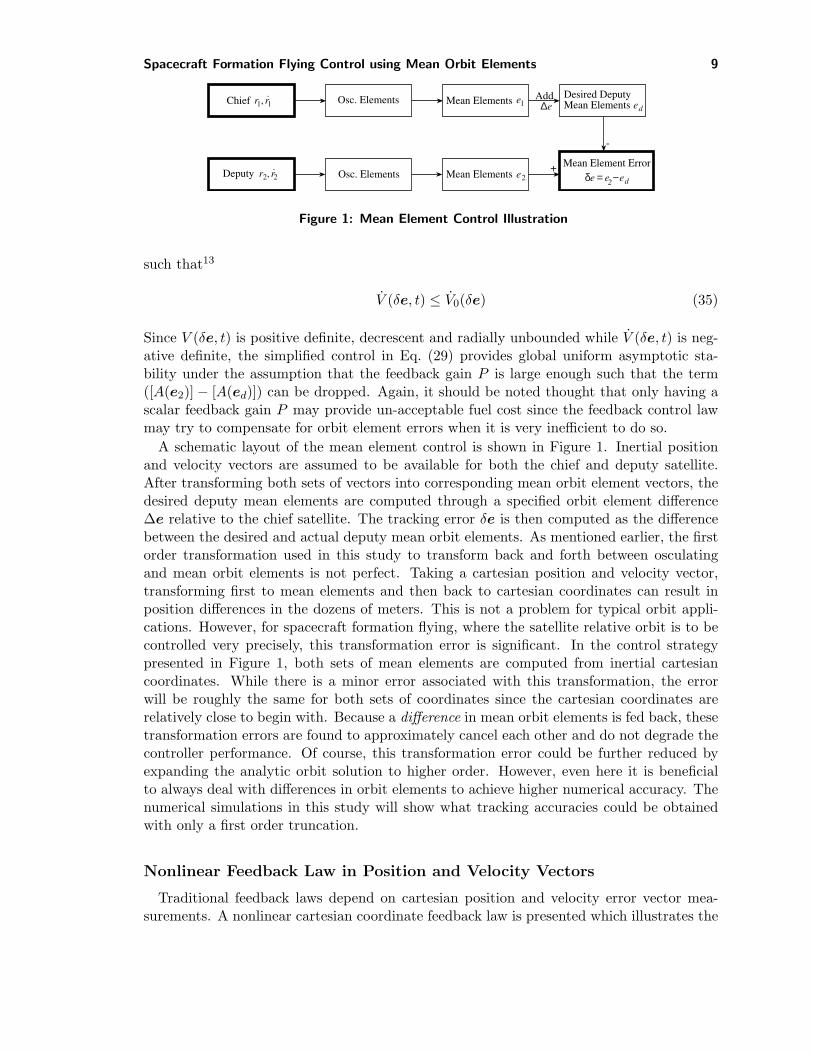
Figure 1: Mean Element Control Illustration

such that13

V (δe, t) ≤ V0(δe) (35)

Since V (δe, t) is positive definite, decrescent and radially unbounded while V (δe, t) is neg-ative definite, the simplified control in Eq. (29) provides global uniform asymptotic sta-bility under the assumption that the feedback gain P is large enough such that the term([A(e2)]− [A(ed)]) can be dropped. Again, it should be noted thought that only having ascalar feedback gain P may provide un-acceptable fuel cost since the feedback control lawmay try to compensate for orbit element errors when it is very inefficient to do so.

A schematic layout of the mean element control is shown in Figure 1. Inertial positionand velocity vectors are assumed to be available for both the chief and deputy satellite.After transforming both sets of vectors into corresponding mean orbit element vectors, thedesired deputy mean elements are computed through a specified orbit element difference∆e relative to the chief satellite. The tracking error δe is then computed as the differencebetween the desired and actual deputy mean orbit elements. As mentioned earlier, the firstorder transformation used in this study to transform back and forth between osculatingand mean orbit elements is not perfect. Taking a cartesian position and velocity vector,transforming first to mean elements and then back to cartesian coordinates can result inposition differences in the dozens of meters. This is not a problem for typical orbit appli-cations. However, for spacecraft formation flying, where the satellite relative orbit is to becontrolled very precisely, this transformation error is significant. In the control strategypresented in Figure 1, both sets of mean elements are computed from inertial cartesiancoordinates. While there is a minor error associated with this transformation, the errorwill be roughly the same for both sets of coordinates since the cartesian coordinates arerelatively close to begin with. Because a difference in mean orbit elements is fed back, thesetransformation errors are found to approximately cancel each other and do not degrade thecontroller performance. Of course, this transformation error could be further reduced byexpanding the analytic orbit solution to higher order. However, even here it is beneficialto always deal with differences in orbit elements to achieve higher numerical accuracy. Thenumerical simulations in this study will show what tracking accuracies could be obtainedwith only a first order truncation.

Nonlinear Feedback Law in Position and Velocity Vectors

Traditional feedback laws depend on cartesian position and velocity error vector mea-surements. A nonlinear cartesian coordinate feedback law is presented which illustrates the


steps necessary to track a prescribed relative orbit expressed in terms of mean orbit elementdifferences. A related nonlinear feedback law is presented in Ref. 14.

The inertial equations of motion of the chief satellite r1 and deputy satellite r2 are

r1 = f(r1) (36)r2 = f(r2) + u (37)

where the chief satellite is assumed to be in a free, uncontrolled orbit and only the deputysatellite is being controlled to maintain the desired relative orbit. The vector function f(r)contains the gravitational acceleration. Expressing the inertial position vector in terms ofinertial components r = (x, y, z) and including the J2 perturbation, this function is definedas

f(r) = − µ

r3

r − J232

(req

r

)2

5x(

zr

)2 − x

5y(

zr

)2 − y

5z(

zr

)2 − 3z

(38)

where r is the scalar orbit radius. Let r2dbe the desired inertial position vector of the

deputy satellite for a J2 invariant relative orbit. The position tracking error δr is thendefined as

δr = r2 − r2d(39)

Using this error vector and its derivative, the positive definite Lyapunov function V isdefined as

V (δr, δr) =12δrT δr +

12δrT [K1]δr (40)

where [K1] is a positive definite 3× 3 position feedback gain matrix. Taking the derivativeof V we find

V = δrT (r2 − r2d+ [K1]δr) (41)

Substituting Eq. (37) and making use of the fact that the desired relative orbit is J2 invariant(i.e. control free), the Lyapunov rate is written as

V = δrT (f(r2)− f(r2d) + u + [K1]δr) (42)

Enforcing V to be equal to the negative definite quantity

V = −δrT [K2]δr (43)

where [K2] is a positive definite 3 × 3 velocity feedback gain matrix, the asymptoticallystabilizing control law u is found to be

u = − (f(r2)− f(r2d))− [K1]δr − [K2]δr (44)

The asymptotic stability property of this control law can be verified by checking the higherorder derivatives of V on the set where V is zero (i.e. evaluated at δr = 0).15 The firstnon-zero higher derivative of V on this set is found to be the third derivative

...V (δr = 0) = −δrT [K1]T [K2][K1]δr < 0 (45)


which is negative definite in δr. Thus the order of the first non-zero derivative is odd andthe control law is asymptotically stabilizing.

Where the mean orbit element feedback law feeds back a difference in the natural orbitelement rates, the cartesian coordinate feedback law in Eq. (44) feedback a difference ingravitational accelerations. Linearizing this difference about the desired motion r2d

(t) wefind

f(r2)− f(r2d) '

[∂f

∂r

]∣∣∣∣r2d

δr = [F (r2d)]δr (46)

Using Eq. (46), the closed-loop dynamics are now written in the linear form as

δr ' [F (r2d)]δr + u (47)

and the control law is linearized as

u ' −([F (r2d)] + [K1])δr − [K2]δr (48)

The matrix [F ] can be written as [F ] = [FKepler] + [FJ2 ] where [FKepler] is the term due tothe inverse square gravitational attraction and [FJ2 ] is the term due to the J2 perturbation.Doing a similar dimensional study of [FKepler] and [FJ2 ], as for [A∗] earlier, the matrix[FKepler] is found to be of order µ/r and [FJ2 ] of order J2µ/r3. Since both J2 and 1/r areroughly 10−3, this means that [FJ2 ] is on the order of 10−9 smaller than [FKepler]. Thismeans that excluding the J2 term in the f(r) calculation will have a negligible effect onthe performance. Therefore the largest component of [F ] is of order µ/r = 101 in metricunits. As the numerical simulations will show, the position feedback gains are typically muchsmaller than this. For the cartesian feedback law, feeding back the difference in gravitationalaccelerations has a large influence on the performance. For example, if the gains are verysmall to allow the maneuver to take several orbit revolutions, then the control effort willstill be large due to this gravitational acceleration difference term. This is in contrast to themean orbit element feedback law where the maneuvers can easily be stretched over severalorbit revolutions.

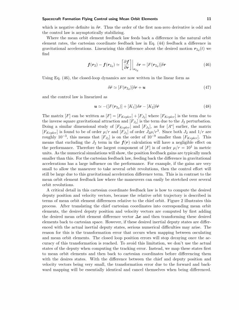
A critical detail in this cartesian coordinate feedback law is how to compute the desireddeputy position and velocity vectors, because the relative orbit trajectory is described interms of mean orbit element differences relative to the chief orbit. Figure 2 illustrates thisprocess. After translating the chief cartesian coordinates into corresponding mean orbitelements, the desired deputy position and velocity vectors are computed by first addingthe desired mean orbit element difference vector ∆e and then transforming these desiredelements back to cartesian space. However, if these desired inertial deputy states are differ-enced with the actual inertial deputy states, serious numerical difficulties may arise. Thereason for this is the transformation error that occurs when mapping between osculatingand mean orbit elements. The closed loop position errors will stop decaying once the ac-curacy of this transformation is reached. To avoid this limitation, we don’t use the actualstates of the deputy when computing the tracking error. Instead, we map these states firstto mean orbit elements and then back to cartesian coordinates before differencing themwith the desires states. With the difference between the chief and deputy position andvelocity vectors being very small, the transformation error due to the forward and back-ward mapping will be essentially identical and cancel themselves when being differenced.


Chief r1, r1 Osc. Elements Mean Elements e1

Desired DeputyMean Elements ed

Osc. ElementsDesired Deputyrd ,rd

Deputy r2, r2 Osc. Elements

Osc. Elements

Mean Elements e2

Deputy r2, r2

δr = r2 − rd δr = r2 − rd

Add ∆e

+-

Figure 2: Tracking Error Computation Logic for Cartesian Coordinate Control

This qualitative observation is consistent with our numerical experiments. The result is anonlinear cartesian coordinate feedback law that is able to establish the J2 invariant orbitand overcome some of the limitations of having a first-order transformation between theosculating and mean orbit elements.

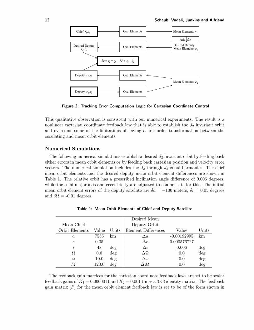
Numerical Simulations

The following numerical simulations establish a desired J2 invariant orbit by feeding backeither errors in mean orbit elements or by feeding back cartesian position and velocity errorvectors. The numerical simulation includes the J2 through J5 zonal harmonics. The chiefmean orbit elements and the desired deputy mean orbit element differences are shown inTable 1. The relative orbit has a prescribed inclination angle difference of 0.006 degrees,while the semi-major axis and eccentricity are adjusted to compensate for this. The initialmean orbit element errors of the deputy satellite are δa = −100 meters, δi = 0.05 degreesand δΩ = -0.01 degrees.

Table 1: Mean Orbit Elements of Chief and Deputy Satellite

Desired MeanMean Chief Deputy Orbit

Orbit Elements Value Units Element Differences Value Unitsa 7555 km ∆a -0.00192995 kme 0.05 ∆e 0.000576727i 48 deg ∆i 0.006 degΩ 0.0 deg ∆Ω 0.0 degω 10.0 deg ∆ω 0.0 degM 120.0 deg ∆M 0.0 deg

The feedback gain matrices for the cartesian coordinate feedback laws are set to be scalarfeedback gains of K1 = 0.0000011 and K2 = 0.001 times a 3×3 identity matrix. The feedbackgain matrix [P ] for the mean orbit element feedback law is set to be of the form shown in


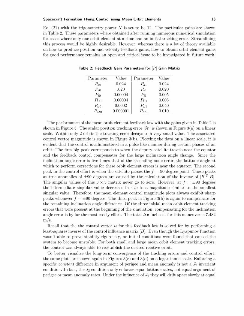
Eq. (21) with the trigonometry power N is set to be 12. The particular gains are shownin Table 2. These parameters where obtained after running numerous numerical simulationfor cases where only one orbit element at a time had an initial tracking error. Streamliningthis process would be highly desirable. However, whereas there is a lot of theory availableon how to produce position and velocity feedback gains, how to obtain orbit element gainsfor good performance remains an open and critical issue to be investigated in future work.

Table 2: Feedback Gain Parameters for [P ] Gain Matrix

Parameter Value Parameter ValuePa0 0.024 Pa1 0.024Pe0 .020 Pe1 0.020Pi0 0.00004 Pi1 0.005PΩ0 0.00004 PΩ1 0.005Pω0 0.0002 Pω1 0.040PM0 0.000001 PM1 0.010

The performance of the mean orbit element feedback law with the gains given in Table 2 isshown in Figure 3. The scalar position tracking error |δr| is shown in Figure 3(a) on a linearscale. Within only 2 orbits the tracking error decays to a very small value. The associatedcontrol vector magnitude is shown in Figure 3(b). Plotting the data on a linear scale, it isevident that the control is administered in a pulse-like manner during certain phases of anorbit. The first big peak corresponds to when the deputy satellite travels near the equatorand the feedback control compensates for the large inclination angle change. Since theinclination angle error is five times that of the ascending node error, the latitude angle atwhich to perform corrections for these orbit element errors is near the equator. The secondpeak in the control effort is when the satellite passes the f= -90 degree point. These peaksat true anomalies of ±90 degrees are caused by the calculation of the inverse of [B]T [B].The singular values of this 3 × 3 matrix never go to zero. However, at f = ±90 degreesthe intermediate singular value decreases in size to a magnitude similar to the smallestsingular value. Therefore, the mean element control magnitude plots always exhibit sharppeaks whenever f = ±90 degrees. The third peak in Figure 3(b) is again to compensate forthe remaining inclination angle difference. Of the three initial mean orbit element trackingerrors that were present at the beginning of the simulation, compensating for the inclinationangle error is by far the most costly effort. The total ∆v fuel cost for this maneuver is 7.482m/s.

Recall that the the control vector u for this feedback law is solved for by performing aleast-squares inverse of the control influence matrix [B]. Even though the Lyapunov functionwasn’t able to prove stability rigorously, no initial conditions were found that caused thesystem to become unstable. For both small and large mean orbit element tracking errors,the control was always able to reestablish the desired relative orbit.

To better visualize the long-term convergence of the tracking errors and control effort,the same plots are shown again in Figures 3(c) and 3(d) on a logarithmic scale. Enforcing aspecific constant difference in argument of perigee and mean anomaly is not a J2 invariantcondition. In fact, the J2 condition only enforces equal latitude rates, not equal argument ofperigee or mean anomaly rates. Under the influence of J2 they will drift apart slowly at equal


time [Orbits]

1 2 3 4

500

1000

1500

2000

2500

3000

3500

4000

(a) Tracking Error Magnitude |δr| (m)

time [Orbits]

1 2 3 4

2e-6

4e-6

6e-6

8e-6

0.00001

0.000012

(b) Control Magnitude (km/s2)

time [Orbits]0 1 2 3 4

1

10

100

1000

(c) Tracking Error Magnitude |δr| (m)

time [Orbits]0 1 2 3 4

1. • 10-10

1. • 10-9

1. • 10-8

1. 10-7

1. 10-6

0.00001

(d) Control Magnitude (km/s2)

Figure 3: Feedback Control Law Performance Comparison

and opposite rates. Having a feedback law attempting to establish the constant differencescauses some of the final tracking errors. Another source of the final tracking errors are thetransformation errors when performing a first order mapping between osculating and meanorbit elements. However, by dealing with differences in orbit elements, the control law isable to converge down to just 2.5 meters from an initial tracking error of over 4000 meters.Similarly, the control effort converges to very small values, but not precisely to zero. Thepeaks seen here are also due the the numerical inverse effect of [B]T [B] at f = ±90 degrees.Had only osculating orbit element tracking errors been fed back, then the performancewould have been noticeably worse. In particular, the final tracking errors would be two tothree orders of magnitude larger. Dealing with mean orbit element we avoid chasing theshort period oscillations and only deal with secular tracking errors.

Figure 3 shows the performance of the cartesian coordinate feedback law. The positiontracking errors take slightly longer than two orbits to decay. The control magnitude shownin Figure 3(b) shows a more continuous control effort compared to the more pulse likecontrol effort demanded by the mean element feedback law. The reason for this is that itcontinuously compensates for any tracking errors, whereas the mean orbit element feedbacklaw, with the particular time-varying gains chosen, does most of its controlling during par-ticular phases of the orbit. The latter lends itself more naturally for multi-orbit revolutioncorrections. If the feedback gains are lowered for the cartesian coordinate feedback law toallow it to use more orbits to perform the correction, then the total control cost starts to


Alo

ng-T

rack

[km

]

Out-

of-

Pla

ne [km

]

Radial [km]

-4

-2

0

2

4

-5

0

5

0

2

4

-4

-2

0

2

4

(a) Mean Orbit Element Feedback Law

-4

-2

0

2

4

-5

0

5

-2

0

2

4

-4

-2

0

2

4

-5

0

5

Along

-Tra

ck [k

m]

Out-

of-

Pla

ne [km

]

Radial [km]

(b) Cartesian Coordinates Feed-back Law

Figure 4: Relative Orbit Trajectories in Rotating Chief LVLH Frame

grow rapidly. The reason for this is due to the relative size of the gravitational accelerationdifference matrix [F (r2d

)]. Even with small gains, it still commands a large cumulativecontrol effort which decreases the effectiveness of multi-orbit corrections with this type ofcontrol law. With the mean orbit element feedback law however, because the element ratedifference matrix [A∗(ed)] is relatively small, only a negligible control effort is required ifthe feedback gains are very small. Therefore the orbit corrections are easier to spread overseveral orbits with the mean orbit element feedback law.

The total control cost for the cartesian feedback law is ∆v = 7.428 m/s, slightly less thanthe element feedback law. The ∆v cost for both types of control laws is rather close most ofthe time. Depending on the initial conditions and feedback gains, either may have a slightlysmaller or larger ∆v cost. As a comparison, the ∆v cost for a two impulse orbit correctionfor the same initial conditions is as low as 6.24 m/s, depending on how long the transit timeis. The feedback control cost is therefore about 20% higher than the two-impulse fuel costfor the given initial conditions.

Whereas the control effort of the mean orbit element feedback law has periodic peaks, thecartesian coordinate feedback law effort is smooth as expected. The position tracking errorsconverge to roughly 1-2 meters in size, slightly less than with the the element feedback law.The control effort during this end game is of the same order of magnitude, but without theperiodic peaks at f = ±90 degrees. For the cartesian coordinate feedback law, dropping theJ2 term from the f(r)vector computation in Eq. (44) has no visible effect on the performanceor convergence.

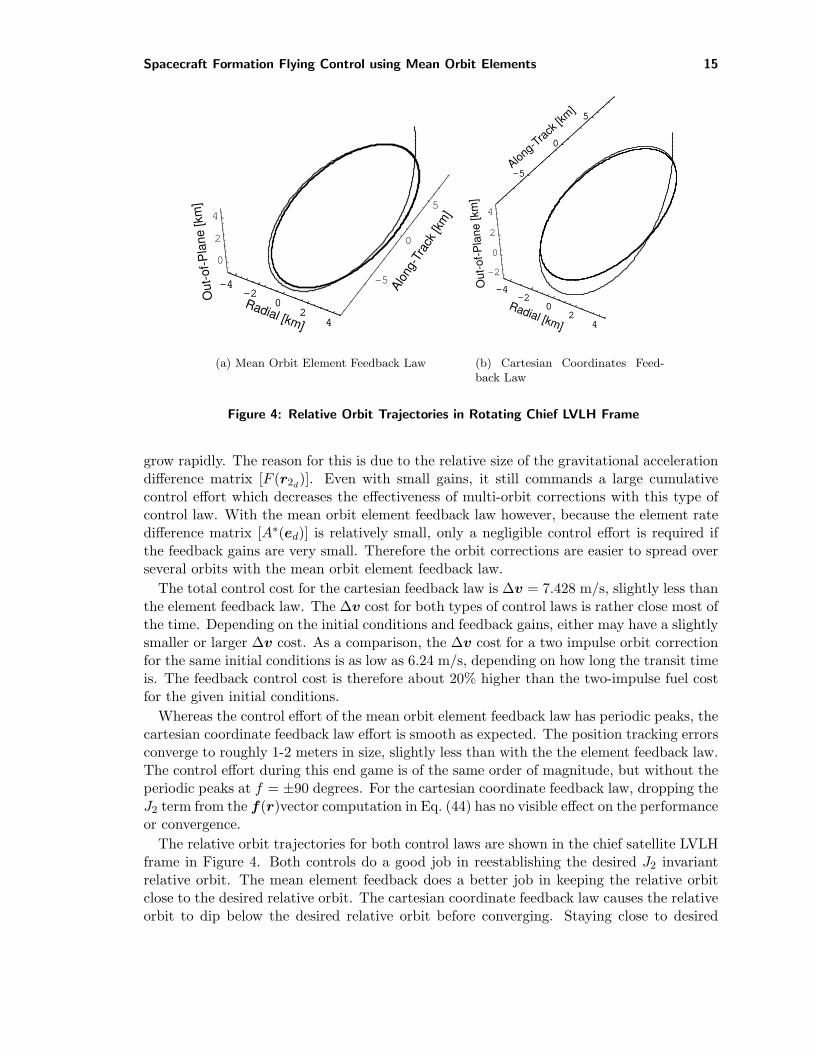
The relative orbit trajectories for both control laws are shown in the chief satellite LVLHframe in Figure 4. Both controls do a good job in reestablishing the desired J2 invariantrelative orbit. The mean element feedback does a better job in keeping the relative orbitclose to the desired relative orbit. The cartesian coordinate feedback law causes the relativeorbit to dip below the desired relative orbit before converging. Staying close to desired


time [Orbits]

1 2 3 4

-0.1

-0.075

-0.05

-0.025

0.025

0.05

0.075

0.1

(a) Semi-Major Axis Error δa (km)

time [Orbits]

1 2 3 4

-0.00005

-0.00004

-0.00003

-0.00002

-0.00001

0.00001

0.00002

(b) Eccentricity Error δe

time [Orbits]

1 2 3 4

0.01

0.02

0.03

0.04

0.05

(c) Inclination Angle Error δi (deg)

time [Orbits]

1 2 3 4

-0.01

-0.0075

-0.005

-0.0025

0.0025

0.005

0.0075

0.01

(d) Ascending Node Error δΩ (deg)

time [Orbits]

1 2 3 4

-0.02

-0.015

-0.01

-0.005

0.005

0.01

(e) Argument of Perigee Error δω (deg)

time [Orbits]

1 2 3 4

-0.01

-0.005

0.005

0.01

0.015

0.02

(f) Mean Anomaly Error δM (deg)

Figure 5: Mean Orbit Element Tracking Errors for (solid) Mean Orbit ElementFeedback Law and (dashed) Cartesian Feedback Law

orbit is beneficial when collision avoidance with other deputy satellites is of consideration.However, the flight paths resulting from either control law do not always differ by thisamount. Often they are very similar in nature.

Where performances of the two control laws differ substantially is in maintaining thedesired mean orbit element of the deputy satellite relative to the chief satellite. Figure 5shows the various mean orbit element tracking errors for both the mean orbit elementfeedback law (solid line) and the cartesian coordinate feedback law (dashed line). Recallthat the initial mean orbit element tracking errors were a semi-major axis error of 0.1 km,


an inclination angle error of 0.05 degrees and an ascending node error of -0.01 degrees.The element control law is able to correct the mean semi-major axis error rather quickly

within a fraction of an orbit. As is expected from Gauss’ variational equations, doing socauses an error in eccentricity, argument of perigee and mean anomaly. This is a generaltrend with the element feedback law. Correcting for one particular orbit element erroralways causes subsequent errors in other orbit elements. Thus, even if only one elementwere off initially, using the element feedback law would correct for this error, but in theprocess the remaining orbit element would experience transient errors. The effect of thetime varying feedback gain matrix [P ] is clearly seen in the inclination angle corrections.They occur whenever the deputy satellite crosses the favorable latitude angles. While e, ωand M do experience transient tracking errors due to compensating for the other elementerrors, these tracking errors remain rather small. This is an advantage of the mean elementtracking law. While it is not able to hold other orbit elements fixed while correcting theinitial mean element tracking errors, it typically does keep them rather close to the desiredvalues. Often this translates into the relative trajectory remaining closer to the desiredtrajectory during the transient phase.

Most of the mean element tracking errors for the cartesian coordinate feedback law arequite different from the mean element tracking errors of the element feedback law. Inparticular, the semi-major axis in not maintained at the desired value at all during thetransient period. This explains the different transient relative orbits that were observedbetween the two feedback laws. As with the element feedback law, temporary tracking errorsare introduced to the eccentricity, argument of perigee and mean anomaly. Further, thesetransient errors are much larger than with the element feedback law. Note the followinginteresting detail. While δω and δM may grow rather large during the maneuver, their sumis maintained close to the desired sum of ωd + Md. This behavior is observed for all initialconditions studied. The mean inclination error time history is similar in profile comparedto the δi(t) of the element feedback law. Major inclination angle correction occur duringthe equatorial orbit regions.

One reason why the cartesian coordinate feedback law performs so well is that the fullnonlinear equations of motion are utilized. In future research it would be interesting tocompare this performance to that of traditional linear control laws such as are used in theclassical rendez-vous problem.

Conclusions

Two nonlinear feedback laws are presented to establish and recursively reestablish adesired J2 invariant relative orbit. While these control laws are applied to the J2 perturbedspacecraft control problem, they are general enough to be used in general orbit control.

The first control law, motivated by orbital mechanics insight, feeds back tracking errorsin mean orbit elements. The advantage here is that the relative orbit errors provide moregeometric information as to what relative orbit perturbations this error will cause than dothe classical position and velocity error expressions. Thus, it is possible to construct thefeedback gain matrix to have the control attempt certain orbit element corrections when itmore efficient or practical. While the general mean orbit element feedback control law doesnot have a rigorous stability proof at this point, numerical studies indicate that it is highlystable and is able to correct for both small and large initial mean orbit element trackingerrors. A rigorous stability proof is provided for a simplified version of the feedback control


law where the feedback gain is a positive scalar. A benefit of this feedback law is that theorbit elements which do not have tracking errors are kept relatively close to the desiredvalues during the maneuver. This makes it simpler to predict what the transient orbit willlook like and consider collision avoidance. Further, it is relatively simple to extend themaneuver over several orbits without increasing the fuel cost by reducing the magnitudesof the feedback gains. The reason for this is that in dealing with errors in orbit elementsversus errors in position and velocity vectors, we are dealing perturbations over very slowlyvarying quantities. Being able to easily extent the maneuvers over multiple orbits impliesthat the thrust requirements can be reduced to fit within practical constraints.

The second control law feeds back traditional cartesian position and velocity errors. Pre-scribing the desired relative orbit in terms of differences in mean orbit elements poses certainnumerical challenges. In particular, a method is shown which partially compensates for thetransformation errors between osculating and mean elements. These transformation errorscan further be reduced by using a higher order truncation of Brouwer’s artificial satellitetheory. The fuel cost for this feedback law is similar to that of the mean orbit element feed-back law and maneuver times are comparable. However, the thrust of the mean elementfeedback law is typically applied is a pulse like manner, whereas the cartesian coordinatefeedback demands a continuous thrust. This means that the element feedback based con-trol could be realized with a hybrid system consisting of conventional fixed-thrust thrustersand variable-thrust pulsed-plasma thrusters. This cartesian coordinate feedback law doesnot lend itself well to be performed over multiple orbits without increasing the fuel costsubstantially. Thus it is more difficult with this method to extend the maneuver time tobring the thrust magnitudes within practical constraints.

Open questions remain how to find proper orbit element feedback gains and how toconstruct the matrix [P (e)] such that the dominant orbit mechanics are better exploited.These critical questions have a significant influence on the performance and feasibility ofthe mean orbit element feedback law. With the tight mission requirements of the currentlyproposed spacecraft formation flying missions, it is critical to exploit the dominant dynamicsthat are present within the control design. The potential payoffs are better insight into thenature of the relative orbit errors, better control over the transient orbits and the ability toextend the corrective maneuvers over an arbitrary number of revolutions.

Acknowledgments

This research was supported by the Air Force Office of Scientific Research under GrantF49620-99-1-0075; the authors are pleased to acknowledge the coordination of Dr. M. Q. Ja-cobs at AFOSR.

References

[1] KAPILA, VIKRAM, SPARKS, ANDREW G., BUFFINGTON, JAMES M., and YAN,QIGUO, “Spacecraft Formation Flying: Dynamics and Control,” Proceedings of theAmerican Control Conference, (San Diego, California), June 1999, pp. 4137–4141.

[2] VASSAR, RICHARD H. and SHERWOOD, RICHARD B., “Formationkeeping for aPair of Satellites in a Cicular Orbit,” Journal of Guidance, Navigatin and Control,Vol. 8, No. 2, March-April 1985, pp. 235 –242.


[3] KONG, EDMUND M., MILLER, DAVID W., and SEDWICK, RAYMOND J., “Opti-mal Trajectories and Orbit Design for Separated Spacecraft Interferometry,” tech. rep.,Massachusetts Institude of Technology, November 1998. SERC #13-98.

[4] FOLTA, DAVID C. and QUINN, DAVID A., “A Universial 3-D Method for Controllingthe Relative Motion of Multiple Spacecraft in Any Orbit,” AIAA/AAS AstrodynamicsSpecialist Conference, (Boston, MA), Aug. 1998. Paper No. 98-4193.

[5] MIDDOUR, JAY W., “Along Track Formationkeeping for Satellites With Low Ec-centricity,” Journal of the Astronautical Sciences, Vol. 41, No. 1, Jan.-March 1993,pp. 19–33.

[6] MELTON, ROBERT G., “Time-Explicit Representation of Relative Motion BetweenElliptical Orbits,” AAS/AIAA Astrodynamics Specialist Conference, (Sun Valley,Idaho), Aug. 1997.

[7] CLOHESSY, W. H. and WILTSHIRE, R. S., “Terminal Guidance System for SatelliteRendezvous,” Journal of the Aerospace Sciences, Vol. 27, No. 9, Sept. 1960, pp. 653–658.

[8] CARTER, THOMAS E., “State Transition Matrix for Terminal Rendezvous Studies:Brief Survey and New Example,” Journal of Guidance, Navigation and Control, 1998,pp. 148–155.

[9] SCHAUB, HANSPETER and ALFRIEND, KYLE T., “J2 Invariant Reference Or-bits for Spacecraft Formations,” Flight Mechanics Symposium, (Goddard Space FlightCenter, Greenbelt, Maryland), May 18-20 1999. Paper No. 11.

[10] BROUWER, DIRK, “Solution of the Problem of Artificial Satellite Theory WithoutDrag,” The Astronautical Journal, Vol. 64, No. 1274, 1959, pp. 378–397.

[11] BATTIN, RICHARD H., An Introduction to the Mathematics and Methods of Astro-dynamcis. New York: AIAA Education Series, 1987.

[12] TAN, ZHAOZHI, BAINUM, PETER M., and STRONG, AVAINE, “The Implemen-tation of Maintaining Constant Distance Between Satellites in Elliptic Orbits,” AASSpaceflight Mechanics Meeting, (Clearwater, Florida), Jan. 2000. Paper No. 00-141.

[13] SLOTINE, JEAN-JACQUES E. and LI, WEIPING, Applied Nonlinear Control. En-glewood Cliffs, New Jersey: Prentice-Hall, Inc., 1991.

[14] QUEIROZ, MARCIO S. De, KAPILA, VIKRAM, and YAN, QIGUO, “Nonlinear Con-trol of Multiple Spacecraft Formation Flying,” Proceedings of AIAA Guidance, Navi-gation, and Control Conference, (Portland, OR), Aug. 1999. Paper No. AIAA 99–4270.

[15] MUKHERJEE, RANJAN and CHEN, DEGANG, “Asymptotic Stability Theorem forAutonomous Systems,” Journal of Guidance, Control, and Dynamics, Vol. 16, Sept.–Oct. 1993, pp. 961–963.

Documents

Spacecraft Formation Flying Control using Mean Orbit Elementsdnc.tamu.edu/drjunkins/yearwise/2000/archival/JAS_48_1_2000... · Spacecraft Formation Flying Control using Mean Orbit