Fomc 20040128 Text Material

Presentation Materials (2.74 MB PDF)

Pages 195 to 238 of the Transcript

Appendix 1: Materials used by Mr. Kos

Page 1

Top panel

Title: Outstanding Debt 1997 - Q3 2003Series: Outstanding MBS, corporate debt, Treasuries, and agency debtHorizon: 1997-2003Description: The amount of MBS, corporate debt and agencies outstanding has been increasing,while the amount of Treasuries outstanding has remained relatively constant.

Source: BMA

Middle panel

Title: Ginnie Mae I 30-Yr Issuance & OutstandingSeries: Monthly issuance and total outstanding amount of 30-year Ginnie MaesHorizon: May 1997-November 2003Description: While monthly issuance of 30-year Ginnie Maes has been increasing, the totaloutstanding has been decreasing.

Source: Lehman Brothers

Bottom panel

Title: 30-Yr Fixed Rate MBS Outstanding: Fannie Mae, Freddie Mac, and Ginnie Mae ISeries: Amount of Fannie Mae, Freddie Mac and Ginnie Mae I 30-year fixed rate MBS outstanding,indexed to 5/1/1997Horizon: May 1997-November 2003Description: The amount of Ginnie Mae I fixed rate MBS outstanding has declined since 1997,while the amount of Fannie Mae and Freddie Mac 30-year fixed rate MBS outstanding has increasedsignificantly.


Appendix 2: Materials used by Mr. Reinhart

Page 1

The Committee's Communications Strategy

Vincent ReinhartJanuary 27, 2004

Class I--FOMCStrictly Confidential (FR)

Page 2Estimated Effects of Committee Communications

This exhibit displays the estimated market effects of various types of Federal Reservecommunications including FOMC policy statements (top-left panel), the semiannual MonetaryPolicy Report (top-right panel), and the FOMC minutes (bottom-left panel), 1997 to present, in basispoints. For each of these types of announcements, a bar chart displays the change in the two-yearTreasury yield in a narrow time interval bracketing the time of the announcement. As summarized ina table (bottom-right panel), FOMC statements tend to have the most significant market impact.

Note: Estimated effects are measured as changes in the on-the-run two-year Treasury yield over an interval surrounding therelease or the start of the Chairman's testimony. Effects of policy statements are adjusted to remove the estimated direct effectof policy surprises.

Top-left panelFOMC Policy Statements

See description above.

Top-right panelMonetary Policy Testimony


Bottom-left panelFOMC Minutes Releases


Bottom-right panelAverage Absolute Effects

Basis points

1. FOMC Statements 6.4

2. FOMC Minutes 2.3

3. Chairman's Testimony 5.0

Memo:

4. Employment Reports 5.2

5. ISM Releases 2.3

6. CPI Releases 3.0

Page 3Roadmap for Today's Discussion

The options confronting the Committee are interrelated. To facilitate the discussion, this briefing willhave five parts:

Overview of optionsAlternative formulas for the risk assessmentExpedited release of the FOMC minutesAn enhanced role for the FOMC projectionsHow the pieces might fit together

Page 4Options Across the Three Communications Issues

Risk assessment Release of the Minutes Role of the Projections

Status quoGradual evolution

- Greater flexibility inassessing risks- Include explicitalternative statementlanguage in theBluebook.

New formulaic language:- Levels - A- Levels - B- Changes

Discontinue the assessmentof risks portion of thestatement.

Status quoRelease approximately

- two weeks after themeeting- three weeks after themeeting- four weeks after themeeting

Status quoIncrease the frequency of theprojections.

- Quarterly- Every regularmeeting

Increase the length of theprojection period.Increase the number ofvariables in the projections.Release of the projections

- In the MPR- In the minutes- In a separatedocument

Page 5Lessons from the Working Group: Formulas for the Risk Assessment

Design Principles for the Risk Assessment Key Questions that were Left Unanswered

The Committee should vote on the exactwording of the risk assessment.

1.

The statement should not hamper the policydiscussion.

2.

The statement should be flexible enough toencompass the Committee members' viewsabout the operation of the economy and theconcepts that can be usefully measured.

3.

The statement should be clear to the public.4.The statement should cover the range offeasible contingencies.

5.

Should the wording of the risk assessment be interms of the levels of output and inflation ortheir changes?

1.

What conditioning assumption for monetarypolicy should be employed?

2.

Over what period should the outlook and risksbe considered?

3.

Design Principles for the Risk Assessment Key Questions that were Left Unanswered

The statement should avoid the use ofpotentially charged terms.

6.

Page 6The "Levels - A" Alternative

[Note: For Pages 6, 7, and 8, emphasis (italic) and strong emphasis (bold) have been added toindicate red and blue text, respectively, in the original document.]

The Committee's assessment of the outlook over thenext several quarters is that real economic activitymay well [fall short of / be about on / exceed] a pathconsistent with the long-run trend of its potential. Overthe same period, inflation may well [fall short of / beabout on / exceed] a path consistent with price stabilityin the long run.

In light of these assessments and its goals of maximumsustainable growth and price stability, the Committeejudges that the risk(s)

of [weak economic activity / unsustainableeconomic activity] / (and) / [undesirably lowinflation / undesirably high inflation] [is aconcern / is of greater concern / are bothconcerns].to both of its long-run goals are balanced.

Stated in terms of levels, with explicit referenceto benchmarks for inflation and output.Silent about the conditioning assumption forpolicy, but based on an assumption of "normal"policy.Horizon is "several quarters," but outcomesare described relative to paths that continuefurther into the future.

Page 7The "Levels - B" Alternative

The Committee's assessment of the outlook is that thelevel of economic activity will likely [fall short of /about attain / remain near / exceed] the long-run trendof its potential in the foreseeable future. Over thesame period, inflation will likely [fall below / aboutattain / remain within / exceed] the range consistentwith price stability in the long run.

In light of these assessments and its goals of maximumsustainable growth and price stability, the Committeejudges that the risk(s)

of [undesirably weak economic activity /unsustainably strong economic activity] / (and)/ [undesirably low inflation / undesirably highinflation] [is a concern / is the greater concern /are both concerns]to both of its long-run goals are balanced

for the foreseeable future.

Stated in terms of levels, with explicit referenceto benchmarks for inflation and output.Silent about the conditioning assumption forpolicy, but based on an assumption of anunchanged policy stance.Horizon is "the foreseeable future."

Page 8The "Changes" Alternative

The Committee's assessment of the outlook is thateconomic growth will likely [fall short of / about attain/ remain near / exceed] its long-run sustainable pace inthe foreseeable future. Over the same period,inflation will likely [fall / remain about the same /rise].

In light of these assessments and its goals of maximumsustainable growth and price stability, the Committeejudges that

economic growth [below / equal to / above] itslong-run sustainable pace / (and) / [falling /stable / rising] inflation [is the greater concern/ is a concern / are both concerns]the risks to the achievement of both of itslong-run goals are balanced

for the foreseeable future.

Stated in terms of changes in output relative topotential and changes in inflation.References to levels and benchmarks would bein the first paragraph.Silent about the conditioning assumption forpolicy, but based on an assumption of anunchanged policy stance.Horizon is "the foreseeable future."

Page 9Some Possible Pitfalls

Measurement

"Long-run trend of potential""Level of potential output""Long-run sustainable pace""Price stability"

Clarity

"Path consistent with…""Foreseeable future"

Conditioning assumption

"Normal" policy"Appropriate" policyUnchanged policy

Page 10Expedited Release of the FOMC Minutes

Pros Cons

Providing more timely information to the publicIncreasing transparency and accountabilityPotential for shortening the policyannouncement

Possible effects on Committee deliberationsPossible effects on the minutes

- Quality- Ability to make conditional statements- Temptation to send signals

Possible inappropriate market responsesAdverse interactions with other aspects ofCommittee communications

- Interaction with the MPR andtestimony- Creating additional news events

Blackout periods

Page 11Enhanced Role for the FOMC Projections

There are several margins over which the Committeecan choose:

Increased frequency (every meeting or everyquarter).Increased length of projection periods.Increased number of variables in the projections

- e.g., core PCE inflation, potentialoutput growth, the "working definition ofprice stability," or the width ofuncertainty bands for the projections.

Separate projections from the Monetary PolicyReport and testimony.

Pros:

Providing more timely information to thepublic.

- Both about the central tendencies andthe range of opinions.

Increasing transparency and accountability.Possible substitute for the risk assessment in thestatement.

Cons:

As a matter of process, should the forecasts be:- Included in the minutes of themeetings?- Revised after the meetings?- Augmented by explanatory text?

The public might not understand the conditionalnature of the projections.Separate publication would create additionalnews events.The Committee's credibility could be impairedif the forecasts turn out to be wrong.

Page 12Options Across the Three Communications Issues


Status quoGradual evolution

- Greater flexibility in

Status quoRelease approximately

- two weeks after the

Status quoIncrease the frequency of theprojections.


assessing risks- Include explicitalternative statementlanguage in theBluebook.

New formulaic language:- Levels - A- Levels - B- Changes

Discontinue the assessmentof risks portion of thestatement.

meeting- three weeks after themeeting- four weeks after themeeting

- Quarterly- Every regularmeeting

Increase the length of theprojection period.Increase the number ofvariables in the projections.Release of the projections

- In the MPR- In the minutes- In a separatedocument

Appendix 3: Materials used by Mr. Kos

Page 1

Top panel

Title: Current U.S. 3-Month Deposit Rates and Rates Implied by Traded Forward Rate AgreementsSeries: 3-month USD Libor, USD 3-month forward rate agreement, USD 6-month forward rateagreement, USD 9-month forward rate agreementHorizon: October 1, 2003 - January 26, 2004Description: Forward rate agreements decline.

Middle panel

Title: Treasury Note YieldsSeries: Yields for 10-year and 2-year Treasury notesHorizon: January 1, 2003 - January 26, 2004Description: Treasury yields decline slightly.

Bottom-left panel

Title: Investment Grade Corporate Debt SpreadSeries: Investment grade corporate debt spreadHorizon: September 1, 2003 - January 26, 2004Description: Investment grade corporate debt spread narrows.


Bottom-right panel

Title: High Yield and EMBI+ SpreadsSeries: Merrill Lynch High Yield Bond Index spread and JP Morgan EMBI Plus Sovereign spreadHorizon: September 1, 2003 - January 26, 2004Description: High yield and EMBI+ spreads narrow.

Source: Merrill Lynch, JP Morgan

Page 2

Top panel

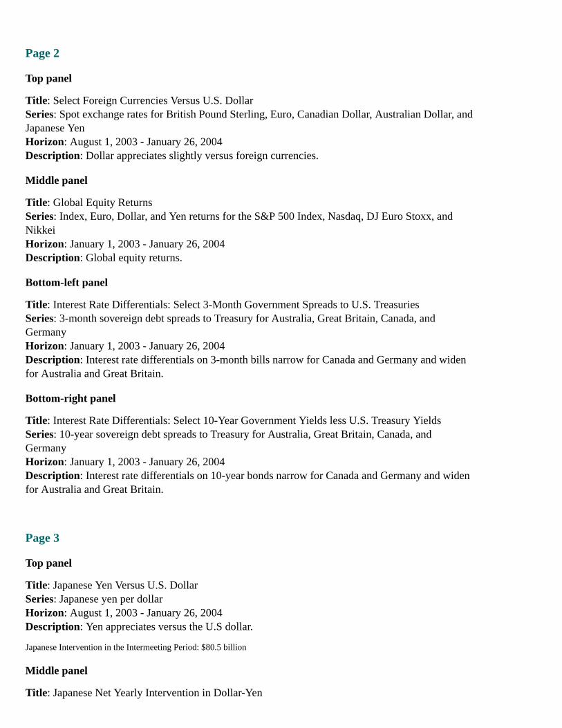
Title: Select Foreign Currencies Versus U.S. DollarSeries: Spot exchange rates for British Pound Sterling, Euro, Canadian Dollar, Australian Dollar, andJapanese YenHorizon: August 1, 2003 - January 26, 2004Description: Dollar appreciates slightly versus foreign currencies.

Middle panel

Title: Global Equity ReturnsSeries: Index, Euro, Dollar, and Yen returns for the S&P 500 Index, Nasdaq, DJ Euro Stoxx, andNikkeiHorizon: January 1, 2003 - January 26, 2004Description: Global equity returns.

Bottom-left panel

Title: Interest Rate Differentials: Select 3-Month Government Spreads to U.S. TreasuriesSeries: 3-month sovereign debt spreads to Treasury for Australia, Great Britain, Canada, andGermanyHorizon: January 1, 2003 - January 26, 2004Description: Interest rate differentials on 3-month bills narrow for Canada and Germany and widenfor Australia and Great Britain.

Bottom-right panel

Title: Interest Rate Differentials: Select 10-Year Government Yields less U.S. Treasury YieldsSeries: 10-year sovereign debt spreads to Treasury for Australia, Great Britain, Canada, andGermanyHorizon: January 1, 2003 - January 26, 2004Description: Interest rate differentials on 10-year bonds narrow for Canada and Germany and widenfor Australia and Great Britain.

Page 3

Top panel

Title: Japanese Yen Versus U.S. DollarSeries: Japanese yen per dollarHorizon: August 1, 2003 - January 26, 2004Description: Yen appreciates versus the U.S dollar.

Japanese Intervention in the Intermeeting Period: $80.5 billion

Middle panel

Title: Japanese Net Yearly Intervention in Dollar-Yen

Series: Japanese yearly intervention in dollar-yenHorizon: 1989 - 2004Description: Year-to-date Japanese intervention $60 billion as of January 24.

Bottom-left panel

Title: TIC Data: Cumulative Foreign Treasury Note and Bill PurchasesSeries: Private and official foreign purchases of Treasury notes and billsHorizon: January 2003 - January 2004Description: Foreign purchases of Treasuries increase.

Bottom-right panel

Title: FRBNY Custody Holdings of Treasury and Agency SecuritiesSeries: Federal Reserve Bank of New York custody holdings of Treasury and agency securitiesHorizon: January 2003 - January 2004Description: Custody holdings of Treasuries and agencies increase.

Page 4

Top panel

Title: Current Euro Area 3-Month Deposit Rates and Rates Implied by Traded Forward RateAgreementsSeries: 3-month Euro Libor, Euro 3-month forward rate agreement, Euro 6-month forward rateagreement, Euro 9-month forward rate agreementHorizon: October 1, 2003 - January 26, 2004Description: Euro forward rate agreements decline.

Middle panel

Title: Japanese Yield CurveSeries: Japanese government yields for 3-month to 10-year securitiesHorizon: N/ADescription: Japanese yield curve steepens.

Bottom panel

Title: Japanese Topix Index and Select Sub-IndicesSeries: Japanese Topix Index, Topix Electronics Sub-Index, Topix Bank Sub-IndexHorizon: January 1, 2003 - January 26, 2004Description: Topix and selected sub-indices increase.

Appendix 4: Materials used by Mr. Slifman

Orders and Shipments of Durable Goods

(Percent change from comparable previous period, seasonally adjusted)

Category2003 2003

Q2 Q3 Q4 Oct. Nov. Dec.

Annual rate Monthly rate

Nondefense capital goods

Orders 12.9 17.9 5.0 2.4 -6.0 0.2

Aircraft 2140.8 36.1 1.1 31.1 -14.5 13.7

Excluding aircraft 3.2 17.1 5.1 1.4 -5.6 -.4

Computers and peripherals 65.1 26.6 0.9 -.8 0.1 2.0

Communications equipment -31.2 80.8 -56.2 16.3 -48.5 -21.3

All other 1.0 7.6 21.0 -.8 2.4 1.4

Shipments 5.7 16.4 7.4 0.3 0.4 -.2

Aircraft 8.6 32.6 -8.5 -9.6 18.8 -13.2

Excluding aircraft 5.6 15.6 8.3 0.8 -.4 0.5

Computers and peripherals 35.8 43.5 3.4 4.6 -2.4 -1.3

Communications equipment -6.5 35.2 7.9 2.8 -1.3 -1.0

All other 2.7 8.4 9.3 -.3 0.2 1.0

Supplementary orders series

Durable goods -.8 17.1 15.9 3.9 -2.3 -.0

Real adjusted durable goods -1.6 17.8 3.1 -2.4

Capital goods 10.8 14.9 9.7 4.7 -5.3 0.2

Nondefense 12.9 17.9 5.0 2.4 -6.0 0.2

Defense -2.1 -3.8 47.2 23.2 -1.3 0.1

r Revised. Return to table

a Advance. Return to table

* Contains industry detail not shown separately. Return to table

Appendix 5: Materials used by Messrs. Slifman, Struckmeyer, and Kamin

Material for Staff Presentation on the Economic OutlookJanuary 28, 2004

STRICTLY CONFIDENTIAL (FR) CLASS I-FOMC**Downgraded to Class II upon release of the February 2004 Monetary Policy Report.

Chart 1Near-Term Developments

Top-left panelPrivate Nonfarm Payroll Employment

The period covered is 2001 through 2003:Q4. The data are represented as bars and expressed asthousands of employees, presented as an average monthly change. A horizontal line is drawn at zero.

r a

*

There are five bars. Approximate values are as follows.

Period Private Nonfarm Payroll Employment

2001 -200,000

2002 -10,000

2003:H1 -5,000

2003:Q3 5,000

2003:Q4 6,000

Top-right panelSales of Light Vehicles

The period covered is 2001 through December 2003. The data are in millions of units and are plottedon a curve.

In 2001:Q1, the curve starts at nearly 14 million, then fluctuates between about 13 million and 14million in the second and third quarters. The curve climbs to about 17.5 million in 2001:Q4, thendecreases to approximately 12.5 million by year-end. The curve increase to about 14 million in2002:Q1; it then dips to about 12.5 million in 2002:Q2, increases to about 15.25 million in 2002:Q3,decreases to about 12 million at the start of 2002:Q4, and climbs to about 15 million by year-end2002. In 2003:Q1, the curve drops to about 12 million, increases to about 15.25 million in 2003:Q2,falls to about 12.5 million in 2003:Q3, then increases to about 15 million by the end of the year.

Middle-left panelReal Retail Sales

The figure shows real retail sales, excluding sales at automobile dealers and building material andsupply stores. The data are represented as 12 bars and are expressed as a percent change at an annualrate. The period covered is 2001 through 2003:Q4, and a horizontal line is drawn at zero.Approximate values are as follows.

Period Real Retail Sales

2001:Q1 about 0.25 percent

2001:Q2 just under zero

2001:Q3 about 3 percent





2002:Q4 just under 6 percent





Middle-right panelOrders and Shipments of Nondefense Capital Goods

The figure shows the orders and shipments of nondefense capital goods, excluding aircraft. The dataare plotted on two curves and represent the three-month moving average, in billions of dollars. Theperiod covered is 2001 through December 2003. One curve is for shipments, and the other curve isfor orders.

The curve for shipments starts in 2001:Q1 at just above 62 billion dollars and falls to about 53 billiondollars in 2001:Q4. In the first quarter of 2002, the curve increases to just above 53 billion dollars,dips to about 53 billion dollars throughout the second quarter, and increases to just above 53 billiondollars in the third quarter. The curve then starts to decrease and drops to approximately 52 billiondollars in 2003:Q1; it then moves upward to end at about 56 billion dollars in December 2003.

The curve for orders starts at about 62 billion dollars in 2001:Q1 and drops to about 51 billion dollarsin the fourth quarter. The curve increases to about 53 billion dollars in 2002:Q1 and dips to about 52billion dollars in 2002:Q2 and remains at about that level through the fourth quarter. The curvemoves generally upward through 2003, ending at about 57 billion dollars in December 2003.

Bottom-left panelNonfarm Business Productivity

Period Percent change, annual rate Forecast

2001 2.88 ND

2002 4.13 ND

2003:H1 4.72 ND

2003:Q3 9.40 ND

2003:Q4 ND 3.28

2004:Q1 ND 3.66

* Percent changes are calculated from end of the preceding period to end of the period indicated. Return to table

Bottom-right panelReal GDP

Percent change, annual rate

2003:Q4 2004:Q1

1. Real GDP 4.8 5.0

Contributions (percentage points):

2. Final sales 3.9 4.5

3. Inventories .8 .5

Chart 2The Longer-Run Outlook

Top-left panelReal GDP

Period Percent Change, Q4/Q4 Forecast

1998 4.51 ND

*

Period Percent Change, Q4/Q4 Forecast

1999 4.70 ND

2000 2.24 ND

2001 -0.04 ND

2002 2.80 ND

2003 4.48 ND

2004 ND 5.28

2005 ND 4.00

Top-right panelMajor Forces Shaping the Outlook

Fiscal policy - stimulative in 2004, slightly restrictive in 2005.Supportive monetary policy.Robust gains in structural productivity.Improved financial conditions for business.Higher stock market.

Middle-left panelFiscal Impetus

Period Percent of GDP Forecast

1998 -0.0 ND

1999 0.3 ND

2000 0.1 ND

2001 0.47 ND

2002 1.04 ND

2003 1.15 ND

2004 ND 1.06

2005 ND -0.18

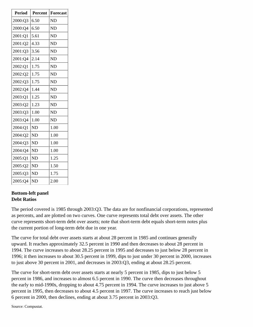
Middle-right panelFederal Funds Rate

Period Percent Forecast

1998:Q1 5.50 ND

1998:Q2 5.50 ND

1998:Q3 5.49 ND

1998:Q4 4.91 ND

1999:Q1 4.75 ND

1999:Q2 4.75 ND

1999:Q3 5.10 ND

1999:Q4 5.38 ND

2000:Q1 5.69 ND

2000:Q2 6.25 ND

Period Percent Forecast

2000:Q3 6.50 ND

2000:Q4 6.50 ND

2001:Q1 5.61 ND

2001:Q2 4.33 ND

2001:Q3 3.56 ND

2001:Q4 2.14 ND

2002:Q1 1.75 ND

2002:Q2 1.75 ND

2002:Q3 1.75 ND

2002:Q4 1.44 ND

2003:Q1 1.25 ND

2003:Q2 1.23 ND

2003:Q3 1.00 ND

2003:Q4 1.00 ND

2004:Q1 ND 1.00

2004:Q2 ND 1.00

2004:Q3 ND 1.00

2004:Q4 ND 1.00

2005:Q1 ND 1.25

2005:Q2 ND 1.50

2005:Q3 ND 1.75

2005:Q4 ND 2.00

Bottom-left panelDebt Ratios

The period covered is 1985 through 2003:Q3. The data are for nonfinancial corporations, representedas percents, and are plotted on two curves. One curve represents total debt over assets. The othercurve represents short-term debt over assets; note that short-term debt equals short-term notes plusthe current portion of long-term debt due in one year.

The curve for total debt over assets starts at about 28 percent in 1985 and continues generallyupward. It reaches approximately 32.5 percent in 1990 and then decreases to about 28 percent in1994. The curve increases to about 28.25 percent in 1995 and decreases to just below 28 percent in1996; it then increases to about 30.5 percent in 1999, dips to just under 30 percent in 2000, increasesto just above 30 percent in 2001, and decreases in 2003:Q3, ending at about 28.25 percent.

The curve for short-term debt over assets starts at nearly 5 percent in 1985, dips to just below 5percent in 1986, and increases to almost 6.5 percent in 1990. The curve then decreases throughoutthe early to mid-1990s, dropping to about 4.75 percent in 1994. The curve increases to just above 5percent in 1995, then decreases to about 4.5 percent in 1997. The curve increases to reach just below6 percent in 2000, then declines, ending at about 3.75 percent in 2003:Q3.

Source: Compustat.

Bottom-right panelCorporate Bond Spreads to Similar Maturity Treasury

The period covered is 1998 through January 26, 2004. The data are plotted on two curves. One curverepresents the 5-year high-yield, and the other curve represents the 10-year BBB. The data are inbasis points, presented weekly.

The 5-year high-yield curve begins at about 400 basis points at the beginning of 1998 and increasesto just above 700 basis points by year-end. The curve continues generally downward and fluctuatesbetween about 500 basis points and just above 500 basis points from midyear 1999 to the start of2000. The curve then fluctuates in a general upward trend to reach about 950 basis points byyear-end 2000. At the start of 2001, the curve declines and fluctuates between approximately 750basis points and just below 900 basis points before increasing to about 1,000 basis points in 2001:Q3.The curve declines to about 675 basis points by the middle of 2002 and increases to just under 1,100basis points in the second half of the year. The curve then fluctuates generally downward, ending atabout 450 basis points on January 26, 2004.

The 10-year BBB curve begins at approximately 80 basis points at the beginning of 1998 andincreases to almost 200 basis points in late 1998 and dips to about 150 basis points and stays therethroughout 1999. The curve then reaches about 200 basis points by mid-2000 and stays near thatpoint until year-end 2000. In 2001, the curve continues generally downward to about 175 basis pointsby midyear, increases to about 225 basis points, and decreases to about 175 basis points by the end ofthe year. The curve fluctuates in an upward trend to reach about 325 basis points by 2002:Q4. It thenfluctuates downward, ending at about 125 basis points on January 26, 2004.

Chart 3Household Sector

Top-left panelReal DPI and PCE Growth

Percent

Period PCE PCE Forecast DPI DPI Forecast

2002 2.72 ND 3.52 ND

2003 3.96 ND 3.72 ND

2004 ND 4.23 ND 4.95

2005 ND 3.95 ND 4.23

Top-right panelSaving Rate

The period covered is 1990 through 2005. The data are represented as a percent of DPI and areplotted on two curves. One curve represents pre-revision, and the other curve represents currentestimates.

The pre-revision curve starts in 1990 just under 8 percent; it then moves generally upward to reachabout 9 percent in 1992, dips to about 8 percent, and rises to about 9 percent at the end of 1993. Thecurve fluctuates downward to just below 6 percent in 1994, after which it increases to about 6.25percent in 1995. The curve continues to fluctuate as it decreases to about 4 percent in 1997, then rises

in 1998 to approximately 5 percent. In 1999, the curve decreases to about 2 percent and increases toapproximately 3 percent in 2000. The curves decreases in 2001 to about 2 percent, climbs to about 4percent, then drops to about 1 percent at the end of 2001. In 2002, the curve rises to about 4 percentand decreases in 2003, ending the year at about 3.5 percent.

The current estimates curve starts in 1990 at about 7 percent; it then fluctuates between about 7 and 8percent through 1992. The curve continues to fluctuate as it decreases to about 4 percent in 1994,then increases to reach just below 6 percent in 1995. The curve then decreases, fluctuating betweenabout 3.5 and 4 percent in 1996 and 1997. It increases to about 4.5 percent in 1998, slides to justunder 2 percent in 1999, and increases to about 3 percent in 2000. The curve then fluctuates in 2001downward to about 1 percent, climbs to about 3 percent, and decreases to nearly 1 percent. In 2002,the curve increases to approximately 3 percent, then dips to just under 2 percent. In 2003, the curveincreases to about 2.25 percent and decreases to just under 2 percent.

The current estimates curve then shows a forecast from 2003:Q4 through 2005, where it increasesthroughout the period, ending at about 3 percent.

Middle panelIs The Saving Rate Too Low?

The BEA, in effect, shifted the goal posts in its most recent comprehensive revision.The current saving rate still is well below the level that many observers often think of as amore normal rate.The target saving rate is a moving target.

It varies over time as the fundamental determinants, such as the wealth-income ratio, thecomposition of income, and real interest rates, change.The current settings of those fundamentals point to a target saving rate for the next yearor two in the neighborhood of 3 percent.

The saving rate rises to 2.8 percent by the fourth quarter of 2005, eliminating the bulk of thegap between actual and target saving.

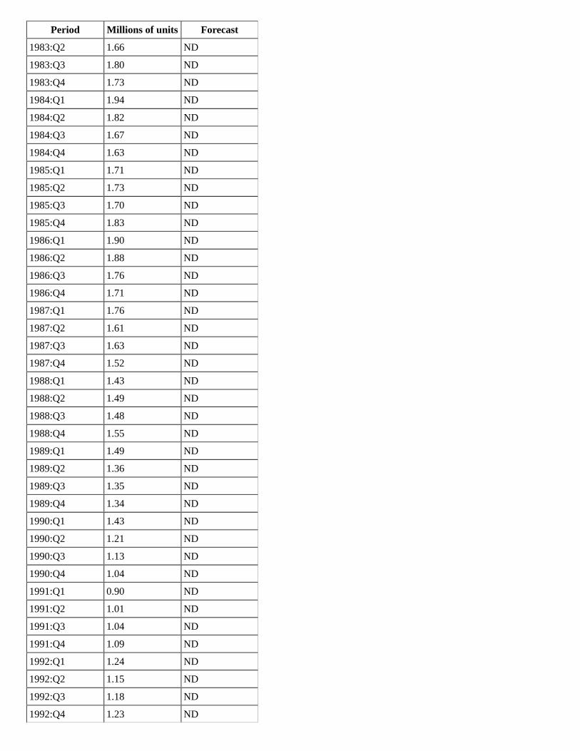
Bottom-left panelPrivate Housing Starts

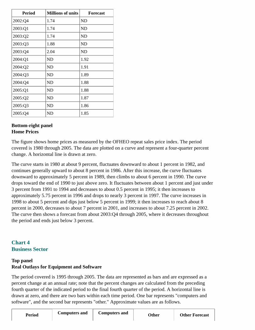
Period Millions of units Forecast

1980:Q1 1.25 ND

1980:Q2 1.06 ND

1980:Q3 1.39 ND

1980:Q4 1.51 ND

1981:Q1 1.37 ND

1981:Q2 1.18 ND

1981:Q3 0.96 ND

1981:Q4 0.87 ND

1982:Q1 0.88 ND

1982:Q2 0.95 ND

1982:Q3 1.12 ND

1982:Q4 1.28 ND

1983:Q1 1.63 ND


1983:Q2 1.66 ND

1983:Q3 1.80 ND

1983:Q4 1.73 ND

1984:Q1 1.94 ND

1984:Q2 1.82 ND

1984:Q3 1.67 ND

1984:Q4 1.63 ND

1985:Q1 1.71 ND

1985:Q2 1.73 ND

1985:Q3 1.70 ND

1985:Q4 1.83 ND

1986:Q1 1.90 ND

1986:Q2 1.88 ND

1986:Q3 1.76 ND

1986:Q4 1.71 ND

1987:Q1 1.76 ND

1987:Q2 1.61 ND

1987:Q3 1.63 ND

1987:Q4 1.52 ND

1988:Q1 1.43 ND

1988:Q2 1.49 ND

1988:Q3 1.48 ND

1988:Q4 1.55 ND

1989:Q1 1.49 ND

1989:Q2 1.36 ND

1989:Q3 1.35 ND

1989:Q4 1.34 ND

1990:Q1 1.43 ND

1990:Q2 1.21 ND

1990:Q3 1.13 ND

1990:Q4 1.04 ND

1991:Q1 0.90 ND

1991:Q2 1.01 ND

1991:Q3 1.04 ND

1991:Q4 1.09 ND

1992:Q1 1.24 ND

1992:Q2 1.15 ND

1992:Q3 1.18 ND

1992:Q4 1.23 ND


1993:Q1 1.17 ND

1993:Q2 1.27 ND

1993:Q3 1.30 ND

1993:Q4 1.43 ND

1994:Q1 1.39 ND

1994:Q2 1.47 ND

1994:Q3 1.45 ND

1994:Q4 1.47 ND

1995:Q1 1.32 ND

1995:Q2 1.29 ND

1995:Q3 1.42 ND

1995:Q4 1.42 ND

1996:Q1 1.46 ND

1996:Q2 1.50 ND

1996:Q3 1.50 ND

1996:Q4 1.42 ND

1997:Q1 1.43 ND

1997:Q2 1.48 ND

1997:Q3 1.46 ND

1997:Q4 1.53 ND

1998:Q1 1.56 ND

1998:Q2 1.57 ND

1998:Q3 1.63 ND

1998:Q4 1.72 ND

1999:Q1 1.71 ND

1999:Q2 1.57 ND

1999:Q3 1.65 ND

1999:Q4 1.66 ND

2000:Q1 1.66 ND

2000:Q2 1.59 ND

2000:Q3 1.50 ND

2000:Q4 1.54 ND

2001:Q1 1.61 ND

2001:Q2 1.63 ND

2001:Q3 1.60 ND

2001:Q4 1.57 ND

2002:Q1 1.72 ND

2002:Q2 1.68 ND

2002:Q3 1.70 ND


2002:Q4 1.74 ND

2003:Q1 1.74 ND

2003:Q2 1.74 ND

2003:Q3 1.88 ND

2003:Q4 2.04 ND

2004:Q1 ND 1.92

2004:Q2 ND 1.91

2004:Q3 ND 1.89

2004:Q4 ND 1.88

2005:Q1 ND 1.88

2005:Q2 ND 1.87

2005:Q3 ND 1.86

2005:Q4 ND 1.85

Bottom-right panelHome Prices

The figure shows home prices as measured by the OFHEO repeat sales price index. The periodcovered is 1980 through 2005. The data are plotted on a curve and represent a four-quarter percentchange. A horizontal line is drawn at zero.

The curve starts in 1980 at about 9 percent, fluctuates downward to about 1 percent in 1982, andcontinues generally upward to about 8 percent in 1986. After this increase, the curve fluctuatesdownward to approximately 5 percent in 1989, then climbs to about 6 percent in 1990. The curvedrops toward the end of 1990 to just above zero. It fluctuates between about 1 percent and just under3 percent from 1991 to 1994 and decreases to about 0.5 percent in 1995; it then increases toapproximately 5.75 percent in 1996 and drops to nearly 3 percent in 1997. The curve increases in1998 to about 5 percent and dips just below 5 percent in 1999; it then increases to reach about 8percent in 2000, decreases to about 7 percent in 2001, and increases to about 7.25 percent in 2002.The curve then shows a forecast from about 2003:Q4 through 2005, where it decreases throughoutthe period and ends just below 3 percent.

Chart 4Business Sector

Top panelReal Outlays for Equipment and Software

The period covered is 1995 through 2005. The data are represented as bars and are expressed as apercent change at an annual rate; note that the percent changes are calculated from the precedingfourth quarter of the indicated period to the final fourth quarter of the period. A horizontal line isdrawn at zero, and there are two bars within each time period. One bar represents "computers andsoftware", and the second bar represents "other." Approximate values are as follows.

Period Computers and Computers and Other Other Forecast

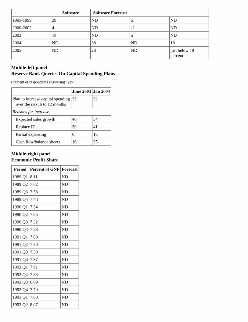
Software Software Forecast

1995-1999 29 ND 5 ND

2000-2002 4 ND -2 ND

2003 18 ND 5 ND

2004 ND 38 ND 18

2005 ND 28 ND just below 10percent

Middle-left panelReserve Bank Queries On Capital Spending Plans

(Percent of respondents answering "yes")

June 2003 Jan 2004

Plan to increase capital spending over the next 6 to 12 months

35 52

Reasons for increase:

Expected sales growth 46 54

Replace IT 39 41

Partial expensing 6 16

Cash flow/balance sheets 16 25

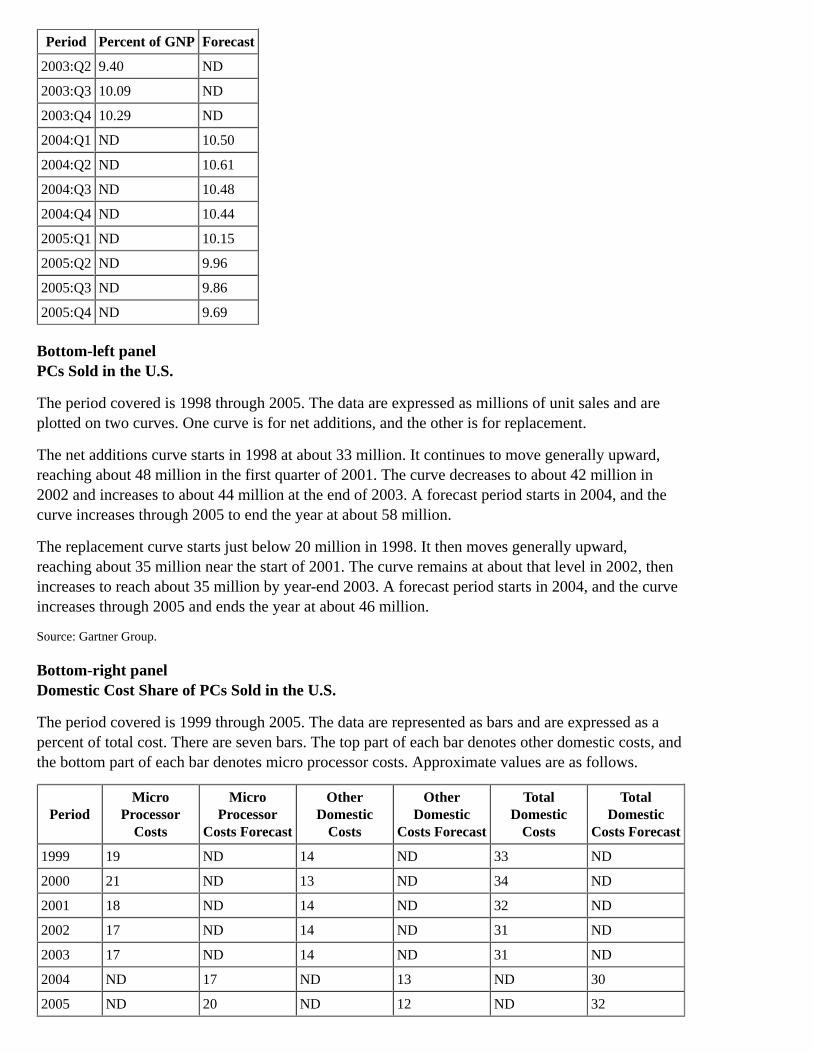
Middle-right panelEconomic Profit Share

Period Percent of GNP Forecast

1989:Q1 8.11 ND

1989:Q2 7.82 ND

1989:Q3 7.58 ND

1989:Q4 7.48 ND

1990:Q1 7.54 ND

1990:Q2 7.85 ND

1990:Q3 7.32 ND

1990:Q4 7.28 ND

1991:Q1 7.69 ND

1991:Q2 7.50 ND

1991:Q3 7.39 ND

1991:Q4 7.37 ND

1992:Q1 7.91 ND

1992:Q2 7.83 ND

1992:Q3 6.69 ND

1992:Q4 7.70 ND

1993:Q1 7.68 ND

1993:Q2 8.07 ND


1993:Q3 8.03 ND

1993:Q4 8.60 ND

1994:Q1 7.59 ND

1994:Q2 8.46 ND

1994:Q3 8.76 ND

1994:Q4 8.99 ND

1995:Q1 8.96 ND

1995:Q2 9.27 ND

1995:Q3 9.66 ND

1995:Q4 9.59 ND

1996:Q1 10.02 ND

1996:Q2 10.00 ND

1996:Q3 9.97 ND

1996:Q4 10.06 ND

1997:Q1 10.26 ND

1997:Q2 10.39 ND

1997:Q3 10.64 ND

1997:Q4 10.38 ND

1998:Q1 9.42 ND

1998:Q2 9.14 ND

1998:Q3 9.17 ND

1998:Q4 8.84 ND

1999:Q1 9.28 ND

1999:Q2 9.22 ND

1999:Q3 9.01 ND

1999:Q4 9.09 ND

2000:Q1 8.62 ND

2000:Q2 8.45 ND

2000:Q3 8.21 ND

2000:Q4 7.94 ND

2001:Q1 7.52 ND

2001:Q2 7.40 ND

2001:Q3 7.06 ND

2001:Q4 8.41 ND

2002:Q1 8.50 ND

2002:Q2 8.64 ND

2002:Q3 8.52 ND

2002:Q4 8.77 ND

2003:Q1 8.61 ND


2003:Q2 9.40 ND

2003:Q3 10.09 ND

2003:Q4 10.29 ND

2004:Q1 ND 10.50

2004:Q2 ND 10.61

2004:Q3 ND 10.48

2004:Q4 ND 10.44

2005:Q1 ND 10.15

2005:Q2 ND 9.96

2005:Q3 ND 9.86

2005:Q4 ND 9.69

Bottom-left panelPCs Sold in the U.S.

The period covered is 1998 through 2005. The data are expressed as millions of unit sales and areplotted on two curves. One curve is for net additions, and the other is for replacement.

The net additions curve starts in 1998 at about 33 million. It continues to move generally upward,reaching about 48 million in the first quarter of 2001. The curve decreases to about 42 million in2002 and increases to about 44 million at the end of 2003. A forecast period starts in 2004, and thecurve increases through 2005 to end the year at about 58 million.

The replacement curve starts just below 20 million in 1998. It then moves generally upward,reaching about 35 million near the start of 2001. The curve remains at about that level in 2002, thenincreases to reach about 35 million by year-end 2003. A forecast period starts in 2004, and the curveincreases through 2005 and ends the year at about 46 million.

Source: Gartner Group.

Bottom-right panelDomestic Cost Share of PCs Sold in the U.S.

The period covered is 1999 through 2005. The data are represented as bars and are expressed as apercent of total cost. There are seven bars. The top part of each bar denotes other domestic costs, andthe bottom part of each bar denotes micro processor costs. Approximate values are as follows.

PeriodMicro

ProcessorCosts

MicroProcessor

Costs Forecast

OtherDomestic

Costs

OtherDomestic

Costs Forecast

TotalDomestic

Costs

TotalDomestic

Costs Forecast

1999 19 ND 14 ND 33 ND

2000 21 ND 13 ND 34 ND

2001 18 ND 14 ND 32 ND

2002 17 ND 14 ND 31 ND

2003 17 ND 14 ND 31 ND

2004 ND 17 ND 13 ND 30

2005 ND 20 ND 12 ND 32

Source: Industry reports, Census Bureau, and staff estimates.

Chart 5Financial Developments

Chart 5 is a three-by-two array of graphs for nominal dollar indexes, dollar exchange rates, ten-yeargovernment bond yields, stock price indexes, bond spreads, and cross-border debt issuance.

Top-left panelNominal Dollar Indexes

Nominal Dollar Indexes on a weekly basis for 2002 to early 2004. The range of the y-axis is [75,115]; index, Jan. 4, 2002 = 100. There is a vertical line in the graph that indicates the time of the June2003 FOMC. The three series are the broad index, which is the trade-weighted average against majorcurrencies and currencies of other important trading partners, the major currencies index, and anindex for other important trading partners. All the series begin at 100. The broad index movesgenerally downward to about 92 by the June 2003 FOMC, and then declines further to about 89 byearly 2004. The major currencies index moves generally downward to about 82 by the June 2003FOMC, and then declines further to about 77 by early 2004. The index of the currencies of otherimportant trading partners moves generally upward to about 107 by early 2003, declines a bit toabout 104 by the June 2003 FOMC, and then fluctuates around 105 through early 2004.

Top-right panelDollar Exchange Rates

Dollar Exchange Rates, foreign currency/dollar, on a weekly basis for 2002 to early 2004. The rangeof the y-axis is [60, 130]; index, Jan. 4, 2002 = 100. There is a vertical line in the graph that indicatesthe time of the June 2003 FOMC. The five series are exchange rate indexes for Mexico, Korea, theUK, Japan, and the euro area. All the series begin at 100. The exchange rate index for Mexico risesgenerally to about 115 by the June 2003 FOMC, and then rises further to about 120 by early 2004.The exchange rate index for Korea declines to just below 90 by mid 2002, and then fluctuates around90 through early 2004. The exchange rate index for the UK declines generally to about 88 by theJune 2003 FOMC, and then falls further to about 80 by early 2004. The exchange rate index forJapan declines to about 90 by the June 2003 FOMC, and then falls further to about 80 by early 2004.The exchange rate index for the euro area declines to about 78 by the June 2003 FOMC, and thenfalls further to about 72 by early 2004.

Middle-left panelTen-Year Government Bond Yields

Ten-Year Government Bond Yields on a weekly basis for the UK, Germany, the United States, andJapan for 2002 through early 2004. The range of the y-axis is [0, 6]; unit is percent. There is avertical line in the graph that indicates the time of the June 2003 FOMC. The yields for the UK,Germany, and the United States all start at about 5 percent and track closely for the entire period. Theyields for the United States rise to about 5½ percent by early 2002, decline to about 3¼ percent bythe June 2003 FOMC, quickly rise to about 4½ percent, and then decline a bit to about 4 percent bythe end of the period. The yields for the UK rise to about 5½ percent by early 2002, decline to about4 percent by the June 2003 FOMC, rise to about 5 percent by late 2003, and then decline a bit toabout 4¾ percent by the end of the period. The yields for Germany rise to about 5½ percent by early2002, decline to about 3¾ percent by the June 2003 FOMC, rise to about 4½ percent by late 2003,

and then decline slightly to just over 4 percent by the end of the period. The yields for Japan start atabout 1½ percent, decline to about ½ percent by the June 2003 FOMC, quickly rise to about 1½percent, and then decline slightly to about 1¼ percent by the end of the period.

Middle-right panelStock Price Indexes

Stock Price Indexes on a weekly basis for emerging markets and industrial countries for 2002through early 2004. The source for the indexes is MSCI. The range of the y-axis is [40, 140]; index,Jan. 4, 2002 = 100. Both series start at 100. The emerging markets index rises to about 115 by early2002, declines to about 80 by late 2002, fluctuates between 80 and 90 through early 2003, then risesto nearly 100 by the June 2003 FOMC and continues to rise to about 130 by the end of the period.The industrial countries index declines to about 70 by late 2002, fluctuates around 70 through early2003, then rises to about 80 by the June 2003 FOMC and continues to rise to about 95 by the end ofthe period.

Bottom-left panelBond Spreads

Bond Spreads on a weekly basis for 2002 through early 2004 for US BBB, EMBI+, and euro-areaBBB. U.S BBB and euro-area BBB are defined as corporate over government debt. For EMBI+, therange of the left y-axis is [300, 1200]; unit is basis points. For US BBB and euro-area BBB, therange of the right y-axis is [50, 350]; unit is basis points. The spreads for US BBB start at just under200 basis points, rise to about 320 basis points by late 2002, fall to about 165 basis points by the June2003 FOMC, and decline further to about 130 basis points by the end of the period. The spreads forEMBI+ start at about 725 basis points, rise to just over 1000 basis points by late 2002, fall to about550 basis points by the June 2003 FOMC, and decline further to about 400 basis points by the end ofthe period. The spreads for euro-area BBB start at just about 170 basis points, rise to about 240 basispoints by late 2002, fall to just over 100 basis points by the June 2003 FOMC, and decline further toabout 80 basis points by the end of the period.

Bottom-right panelCross-border Debt Issuance

Cross-border Debt Issuance on a quarterly basis for industrial countries and emerging markets for1996-2003. The source for the series is Dealogic (Bondware, Loanware). The range of the righty-axis, which measures industrial countries, is [300, 900]; unit is billions of dollars. The range of theleft y-axis, which measures emerging markets, is [15,75]; unit is billions of dollars.. The series forindustrial countries starts at about $350 billion, and, with considerable volatility, rises to about $800billion dollars by end-2003. The series for emerging markets starts at about $35 billion, rises to highsof about $60-$65 billion dollars in late 1996 through late 1997, and then, with considerable volatility,declines to about $30 billion dollars by end-2003.

Chart 6Foreign Outlook

Chart 6 is a three-by-two array of panels including a table on real GDP growth for industrialcountries, and graphs on global trade and IP, oil and non-fuel commodity prices, consumer priceinflation, euro-area industrial sector indicators, and Japanese unemployment and core machineryorders.

Top-left panelReal GDP Growth: Industrial Countries

Real GDP Growth: Industrial Countries (Percent, SAAR) for 2003:H1 (actual), 2003:H2 (estimated),2004 (forecast) and 2005 (forecast).

Percent, SAAR

2003

2004 2005H1 H2

1. Total foreign 0.6 3.9 3.8 3.5

2. Indust. countries 0.7 2.4 2.9 2.8

of which:

3. Euro Area -0.2 1.8 2.4 2.2

4. Japan 2.0 2.4 2.0 1.8

5. Canada 0.6 2.4 3.4 3.3

6. United Kingdom 1.5 3.4 3.0 2.5

* Years are Q4/Q4; half years are Q2/Q4 or Q4/Q2. Return to text

** Aggregates weighted by shares of U.S. exports. Return to table

Top-right panelGlobal Trade and IP

Global Trade and IP on a monthly basis for 2001 through October 2003. The range of the left y-axis,which measures IP as an index, Jan. 2001=100, is [95, 102]. The range of the right y-axis, whichmeasures exports in billions of dollars, is [280, 400]. The index for IP begins at 100, falls to about 96by end-2001, and then rises to slightly over 101 by October 2003. Exports start at about $330 billion,fall to about $290 billion by end-2001, and then rise to about $390 billion by October 2003. The twoseries track fairly closely for the entire period.

* United States and 32 trading partners. IP weighted by 2002 GDP in dollars. Hong Kong and Indonesia IP throughSeptember. Return to text

Middle-left panelOil and Non-fuel Commodity Prices

Oil and Non-fuel Commodity Prices on a monthly basis for 2001-2003 (actual) and for 2004-2005(forecast). The range of the left y-axis, which measures non-fuel commodities as an index, Jan.2001=100, is [80, 130]. The range of the right y-axis, which measures the WTI spot price in dollarsper barrel, is [16, 40]. The non-fuel commodities index is comprised of IMF component indexesweighted by U.S. import shares. The index for non-fuel commodities begins at 100, falls to about 90by late 2001, rises to about 117 by end-2003, and then declines slightly to about 114 by the end ofthe forecast period. The WTI spot price starts at about $30 per barrel, falls to just below $20 perbarrel by end-2001, rises with marked volatility to nearly $34 per barrel by end-2003 (the riseincludes a spike to about $36 per barrel at the beginning of 2003); the WTI spot price then declinesto just under $28 per barrel by the end of the forecast period. The two series track reasonably closelyfor 2001-2003, although the WTI spot price is much more volatile; the series then diverge somewhatduring the forecast period, with the WTI spot price showing more of a decline than the non-fuelcommodities.

Middle-right panel

*

**

*

Consumer Price Inflation

Consumer Price Inflation (four-quarter percent change) on a quarterly basis for 2001-2003 (actual)and 2004-2005 (forecast) for Latin America, the industrial countries, and Asia. The three aggregatesare weighted by shares in U.S. non-oil imports. The range of the y-axis is [-1, 8]. The percent changefor Latin America starts at just over 7 percent, falls to just over 5 percent by early 2002, rises toabout 7 percent by early 2003, declines to about 4½ percent by end-2003, and then further declines toabout 3½ percent by the end of the forecast period. The percent change for industrial countries startsat just over 1½ percent, immediately rises to just over 2 percent, falls to about 1 percent by late 2001,rises to about 2½ percent by early 2003, falls to about 1 percent by end-2003, further declines toabout ¾ percent by early 2004, and then rises to about 1¼ percent by mid-2004 and stays therethrough the end of the forecast period. The percent change for Asia starts at just under 1½ percent,falls to 0 percent by early 2002, rises to about 1½ percent by end-2003, further rises to about 2percent by mid-2004, declines to about 1½ percent by early 2005, and stays there through the end ofthe forecast period.

Bottom-left panelEuro Area - Industrial Sector Indicators

Euro Area - Industrial Sector Indicators on a monthly basis for 2001 through late 2003/early 2004.The range of the left y-axis, which measures euro-area IP as an index, Jan. 2001=100, is [96, 101].The range of the right y-axis, which measures German Ifo as an index, Jan. 2001=100, is [85, 103].The euro-area IP index is a three-month moving average. The index for euro-area IP begins at 100,rises marginally and then falls to just below 97 by end-2001, rises to about 98½ by end-2002,declines to about 97¾ by mid-2003, and then rises to about 98¾ by November 2003. German Ifostarts at 100, falls to about 87 by late 2001, rises to about 94 by mid-2002, falls to about 89 by early2003, and then rises to nearly 100 by January 2004.

Bottom-right panelJapan

Graph "Japan" plots the unemployment rate and core machinery orders on a monthly basis for 2001through November 2003. The range of the left y-axis, which measures the unemployment rate inpercent, is [4.6, 5.6]. The range of the right y-axis, which measures core machinery orders as anindex, Jan. 2001=100, is [75, 105]. The unemployment rate starts at 4.8 percent, immediately falls toabout 4.7 percent, rises to about 5.4 percent by late 2001, fluctuates between about 5.3-5.5 percentthrough early 2003, and then declines to about 5.2 percent by November 2003. Core machineryorders start at 100, and, with marked volatility, rise to about 103 by mid-2001, fall steeply to about77 by early 2002, and rise to about 95 by November 2003.

Chart 7Emerging Market Countries

Chart 7 is a three-by-two array of panels including a table on real GDP growth, and graphs onworldwide semiconductor shipments and Asian IP, China, exports by developing Asia excludingChina, U.S. imports from Asia, and Mexico.

Top-left panelReal GDP Growth

Real GDP Growth (Percent, SAAR) for 2003:H1 (actual), 2003:H2 (estimated), 2004 (forecast), and2005 (forecast).

Percent, SAAR

2003

2004 2005H1 H2

1. Total developing 0.5 6.1 5.1 4.6

2. Developing Asia -0.6 11.0 5.7 5.4

of which:

3. China 6.3 13.6 8.3 7.7

4. Korea -2.2 4.8 5.2 5.2

5. Latin America 0.9 2.0 4.8 4.0

of which:

6. Mexico 1.6 1.0 5.2 4.2

7. Brazil -4.0 2.8 3.5 3.5

* Years are Q4/Q4; half years are Q2/Q4 or Q4/Q2. Return to text

** Aggregates weighted by U.S. exports. Return to table

Top-right panelWorldwide Semiconductor Shipments and Asian IP

Worldwide Semiconductor Shipments and Asian IP on a monthly basis for 1999 through late 2003.The range of the left y-axis, which measures total semiconductor shipments in billions of chips, is [0,40]. The range of the right y-axis, which measures Asian IP as an index, June 1996=100, is [100,140]. Asian IP is weighted by U.S. exports and includes Malaysia, the Philippines, Singapore, SouthKorea, Taiwan, and Thailand. Total semiconductor shipments start at about 22 billion chips, rise toabout 32 billion chips by late 2000, fall to about 23 billion chips by late 2001, and then rise to about33 billion chips by November 2003. Asian IP starts at about 102, rises to nearly 130 by late 2000,falls to about 118 by late 2001, and then rises to about 138 by October 2003. From late 2000 on, thetwo series track fairly closely.

Middle-left panelChina

Graph "China" plots CPI inflation as a line chart on a quarterly basis for 1999-2003, and it plots thetrade balance as a bar chart on an annual basis for 1999-2003. The range of the left y-axis, whichmeasures the trade balance in billions of dollars, is [-12, 36]. The range of the right y-axis, whichmeasures CPI inflation in terms of four-quarter percent change, is [-3.0, 9.0]. CPI inflation starts atabout -1.5 percent, falls immediately to about -2 percent, rises to 0 percent in early 2000, risesfurther to just over 1.5 percent in early 2001, declines to 0 percent in late 2001, falls further to about-1.3 percent in early 2002, rises to 0 percent in late 2002, and rises further to nearly 3 percent byend-2003. Approximate values for the annual trade balance figures, in billions of dollars, for1999-2003 are as follows: 29, 24, 23, 30, 25.

Middle-right panelExports by Developing Asia ex. China

Exports by Developing Asia excluding China, on a quarterly basis for 1999-2003; Developing Asia

*

**

excluding China includes Hong Kong, Korea, Malaysia, the Philippines, Singapore, Taiwan, andThailand. The graph shows exports to the U.S., to the European Union (EU), and to China. 2003:Q4data are through November for exports to the U.S. and to China and through October for exports tothe EU. The range of the y-axis is [70, 210]; unit is billions of dollars, AR. Exports to the U.S. startat just over $150 billion, rise to about $200 billion by late 2000, decline to about $150 billion by late2001, and then range from about $150-$170 billion, ending just below $170 billion at the end of theperiod. Exports to the EU start just below $110 billion, rise to about $130 billion by late 2000,decline to about $100 billion by late 2001, and then rise to just under $130 billion by the end of theperiod. Exports to China start at just under $80 billion, rise to about $110 billion by mid-2000,fluctuate between $100-$110 billion through end-2001, and then rise steeply to just over $200 billionby the end of the period.

Bottom-left panelU.S. Imports from Asia

U.S. Imports from Asia on a quarterly basis for 2000-2003. The graph shows total U.S. imports fromAsia as a line graph, with shaded areas beneath the line to show the proportion of imports fromChina (orange shading), Developing Asia excluding China (tan shading), and Japan (blue shading).2003:Q4 data are through October and November. Developing Asia excluding China includes HongKong, Indonesia, Korea, Malaysia, the Philippines, Singapore, Taiwan, and Thailand. The range ofthe y-axis is [0, 550]; unit is billions of dollars, AR. Total U.S. imports from Asia start at about $375billion, rise to about $460 billion by mid-2000, fall to about $350 billion by early 2002, rise to about$425 billion by mid-2002, decline to about $375 billion in early 2003, and then rise to about $460billion by the end of the period. The shading beneath the line for total exports shows imports fromChina, Developing Asia excluding China, and Japan to each comprise about 1/3 of the totalthroughout the entire period. From the beginning of the period to the end of the period, theproportion of imports from China increases slightly, the proportion of imports from Japan decreasesslightly, and the proportion of imports from Developing Asia excluding China remains about thesame.

Bottom-right panelMexico

Graph "Mexico" plots Mexican exports, Mexican IP, and U.S. IP on a monthly basis for 2000through late 2003. The range of the left y-axis, which measures Mexican exports in billions ofdollars, is [12.0, 15.0]. The range of the right y-axis, which measures Mexican IP and U.S. IP each asan index, Jan. 2000=100, is [95, 105]. Mexican exports, with some volatility, start at just over $13billion, rise to about $14.7 billion by late 2000, fall to about $12.3 billion by late 2001, rise to about$13.8 billion by early 2002, fluctuate between $13.3-$13.9 billion through mid-2003, and then rise toabout $14.5 billion by November 2003. U.S. IP starts at 100, rises to about 102 by mid-2000, falls toabout 96 by late 2001, rises to about 98 by mid-2002, declines to about 97 by mid-2003, and thenrises to nearly 100 in December 2003. Mexican IP starts at 100, immediately dips to about 99, risesto nearly 103 by late 2000, falls to about 96 by late 2001, rises to nearly 99 by early 2002, declines toabout 96 by late 2003, and then rises to about 98 in November 2003.

Chart 8U.S. External Outlook

Chart 8 consists of five panels including graphs on real exports and imports, real GDP of U.S. and

total foreign countries, the real exchange rate outlook, and the current account, and a table onfinancial flows.

Top-left panelReal Exports and Imports

Real Exports and Imports as a bar chart for 2002 (actual), 2003:H1 (actual), 2003:H2 (projected),2004 (projected), and 2005 (projected). The range of the y-axis is [-5, 15]; unit is percent change,SAAR. Years are Q4/Q4; half years are Q2/Q4 or Q4/Q2. Approximate values for the five periodsare as follows.

Percent change, SAAR

20022003

2004 2005H1 H2

Exports (blue) 3 -2 13 12 11

Imports (red) 9 1 6 9 8

Top-right panelReal GDP

Real GDP for the U.S. and total foreign countries as a bar chart for 2002 (actual), 2003:H1 (actual),2003:H2 (projected), 2004 (projected), and 2005 (projected). Real GDP for total foreign countries iscalculated using U.S. export weights. The range of the y-axis is [0, 7]; unit is percent change, SAAR.Years are Q4/Q4; half years are Q2/Q4 or Q4/Q2. Approximate values for the five periods are asfollows.

Percent change, SAAR

20022003

2004 2005H1 H2

U.S. (red) 2.9 2.5 6.4 5.3 4.0

Foreign (blue) 2.8 0.5 3.8 3.7 3.5

Middle-left panelReal Exchange Rate Outlook

Real Exchange Rate Outlook for 2002 through 2003 (actual), along with the January 2004Greenbook forecast from early 2004 through 2005 and the June 2003 Greenbook forecast formid-2003 through 2004. The range of the y-axis is [85, 105]; index, 2001:Q1 = 100. The actualbroad real exchange rate starts at about 103, and declines to about 90 by end-2003. The January 2004Greenbook forecast starts at about 90 in early 2004 and declines to about 88 by the end of 2005. TheJune 2003 Greenbook forecast starts at about 95 in mid-2003 and declines to about 93 by the end of2004.

Middle-right panelCurrent Account

Current Account in terms of percent of GDP and in terms of level (billions of dollars) for 1995through late 2003 (actual) and for late 2003 through 2005 (forecast). The range of the left y-axis,measured in terms of percent of GDP, is [-7, 1]. The range of the right y-axis, measured in terms oflevel or billions of dollars, is [-700, 100]. The graph shows the current account to be in deficit for the

entire period, and the two series track closely for the entire period. The current account in terms oflevel starts at a deficit of about $100 billion, which widens to about $550 billion by late 2003. Theforecast shows the deficit widening further, to about $600 billion by end-2005. The current accountin terms of percent of GDP starts at a deficit of about 1½ percent of GDP, which widens to a deficitof about 5 percent of GDP by end-2002. The forecast shows the deficit remaining at about 5 percentof GDP through end-2005.

Bottom panelFinancial Flows

Billions of Dollars, SAAR

2002 2003:H1 2003:Q3 2003:Q4*

1. Current account -481 -556 -540 NA

2. Official capital, net 88 194 170 247

3. Private capital, net 440 387 323 NA

Of which:

4. Foreign purchases of U.S. securities 408 418 246 309

5. U.S. purchases of foreign securities 16 -37 -116 -62

6. Foreign DI in U.S. 40 114 33 NA

7. U.S. DI abroad -138 -129 -150 NA

* October and November. Return to table

Chart 9Alternative Dollar Scenarios

Chart 9 consists of five panels including a graph of the real exchange rate, a panel with worddescriptions of the three different dollar scenarios, and graphs of real U.S. GDP growth, foreign realGDP growth, and the U.S. current account balance. In all the panels in this chart, Scenario 1 is asolid red line, Scenario 2 is a dashed red line, and Scenario 3 is a dotted blue line.

Top panelReal Exchange Rate

Real Exchange Rate as a broad index for 1983-2003 (actual) and 2004-2005 (forecast). The range ofthe y-axis is [70, 115]; index, 2002:Q1 = 100. The broad index begins just below 100, rises to about113 by early 1985, declines to about 77 by early 1995, rises to about 98 by early 2001, stays therethrough 2002, and then declines to about 89 by end-2003. The January 2004 Greenbook forecastshows the broad index declining further to about 85 by the end of the period. Scenario 1 forecasts thebroad index dropping sharply to about 78 in early 2004 and then declining further to about 75 by theend of the period. Scenario 2 forecasts the broad index dropping sharply to about 78 in early 2004and remaining at that level through the end of the period. Scenario 3 forecasts the broad index risingto about 94 in early 2004 and then declining to about 92 by the end of the period.

Middle-left panelDollar Scenarios

Scenario 1: Dollar decline triggered by higher foreign growth

Scenario 2: "Disorderly correction"Same dollar shock as aboveStock prices fall 12%10-year Treasury yields rise 50 bp

Scenario 3: Dollar appreciation triggered by strong U.S. growth

Middle-right panelReal U.S. GDP Growth

Real U.S. GDP Growth on a semi-annual basis for 2003 (actual) and 2004-2005 (forecast). The rangeof the y-axis is [2, 7]; unit is percent. GDP growth starts at about 2½ percent in 2003:H1 and risessharply to about 6½ percent in 2003:H2. The January 2004 Greenbook forecast shows GDP growthdeclining to just under 4 percent by 2005:H2. Scenario 1 forecasts GDP growth to decline to about4¾ percent by 2005:H2. Scenario 2 and Scenario 3, tracking closely but not exactly, forecast GDPgrowth to decline to about 3¾ percent by 2005:H2.

Half years are Q2/Q4 or Q4/Q2.

Bottom-left panelForeign Real GDP Growth

Foreign Real GDP Growth on a semi-annual basis for 2003 (actual) and 2004-2005 (forecast). Therange of the y-axis is [0, 5½]; unit is percent. GDP growth starts at about ½ percent in 2003:H1 andrises sharply to nearly 4 percent in 2003:H2. The January 2004 Greenbook forecast shows GDPgrowth declining slightly to about 3½ percent by 2005:H2. Scenario 1 forecasts GDP growth to riseto about 5¼ percent by 2005:H1 and then to decline to about 4¾ percent by 2005:H2. Scenario 2forecasts GDP growth to decline to about 3 percent by 2005:H2. Scenario 3 forecasts GDP growth torise slightly to about 4 percent by 2004:H1 and then to decline to about 3¾ percent by 2005:H2.

Half years are Q2/Q4 or Q4/Q2.

Bottom-right panelU.S. Current Account Balance

U.S. Current Account Balance on a semi-annual basis for 2003 (actual) and 2004-2005 (forecast).The range of the y-axis is [-700, -450]; unit is billions of dollars. The graph shows the U.S currentaccount to be in deficit for the entire period. The deficit starts at about $550 billion in 2003:H1 andnarrows to about $525 billion by 2003:H2. The January 2004 Greenbook forecast shows the deficitwidening to nearly $600 billion by 2005:H2. Scenario 1 forecasts the deficit to widen to about $550billion in 2004:H1 and then to narrow to about $450 billion by 2005:H2. Scenario 2 forecasts thedeficit to widen to about $560 billion in 2004:H1 and then to narrow to about $510 billion by2005:H2. Scenario 3 forecasts the deficit to widen to about $625 billion by 2005:H2.

Chart 10Labor Markets

Top-left panelCyclical Comparison of Nonfarm Payroll Employment

The figure's x-axis shows periods from negative 8 to positive 16, with a trough shown at zero. They-axis represents an index (trough equals 100). The data are plotted on three curves. The first curve

represents the average history and includes 1954:Q2, 1958:Q2, 1961:Q1, 1970:Q4, 1975:Q1, and1982:Q4 troughs. The second curve represents the 1991:Q1 recession, and the third curve representsthe 2001:Q4 recession.

The average history curve starts at about 100 on the index on the y-axis in the negative 8 period; itthen increases to just above 102 at about negative 4, dips to about 100 at zero, and increases to about106 at about positive 8. The average history curve then enters a forecast period and increases to justabove 110 at positive 16.

The curve for the 1991:Q1 recession starts just above 98 on the index on the y-axis in the negative 8period. It then increases to about 101 at negative 3, dips to 99 at positive 3, then increases to about101 at positive 8. The 1991:Q1 recession curve then enters a forecast period and increases to about107 at positive 16.

The curve for the 2001:Q4 recession starts at just below 100 on the index on the y-axis at aboutnegative 8. It then increases to about 101 at negative 3 and decreases to about 99 at positive 1 andremains at about that level through positive 8. The 2001:Q4 recession curve then enters a forecastperiod and increases to about 104 at positive 16.

Top-right panelStructural Multifactor Productivity

Percent change, Q4/Q4

Period Dec. GB Dec. GB Forecast Jan. GB Jan. GB Forecast

2002 2.0 ND 2.4 ND

2003 2.4 ND 2.9 ND

2004 ND 1.6 ND 2.1

2005 ND 1.6 ND 1.7

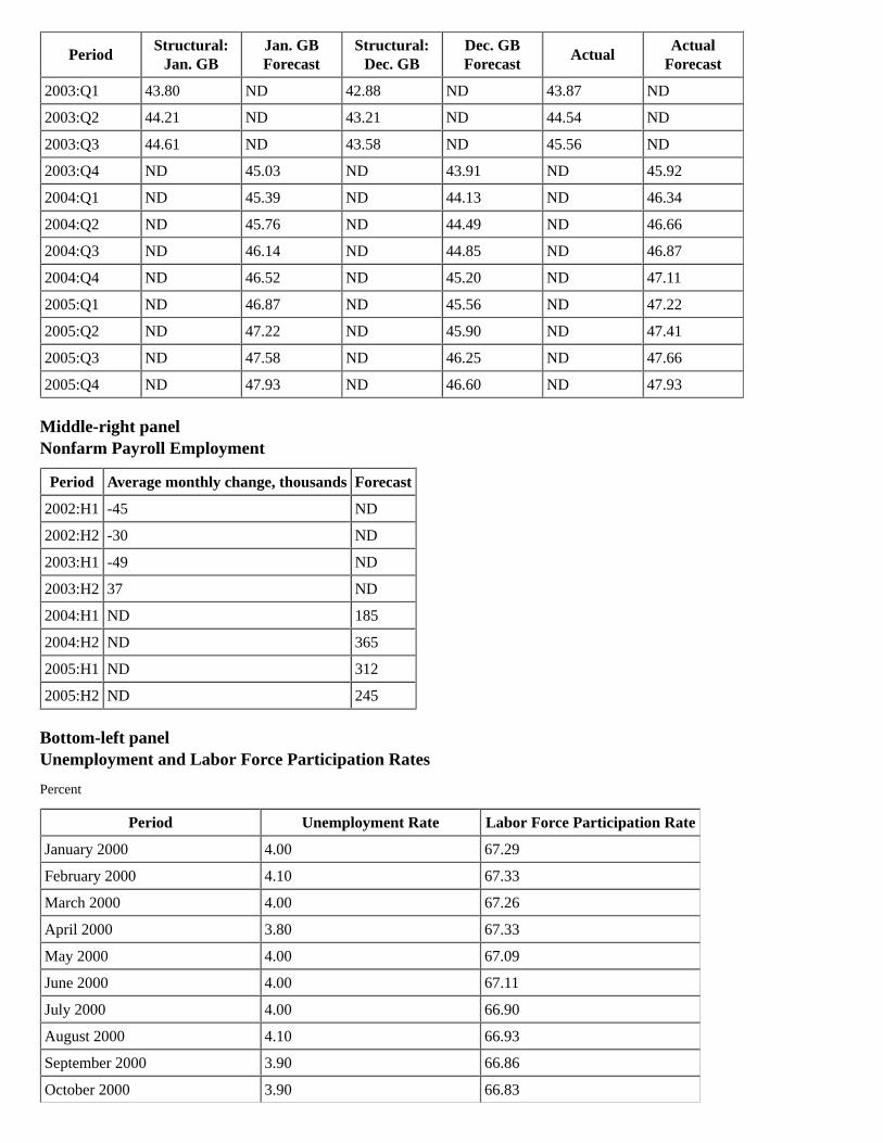
Middle-left panelActual Labor Productivity

Chained (2000) dollars per hour

PeriodStructural:

Jan. GBJan. GBForecast

Structural:Dec. GB

Dec. GBForecast

ActualActual

Forecast

2000:Q1 39.78 ND 39.70 ND 39.61 ND

2000:Q2 40.05 ND 39.98 ND 40.33 ND

2000:Q3 40.33 ND 40.24 ND 40.31 ND

2000:Q4 40.61 ND 40.54 ND 40.63 ND

2001:Q1 40.96 ND 40.92 ND 40.62 ND

2001:Q2 41.31 ND 41.13 ND 40.96 ND

2001:Q3 41.67 ND 41.55 ND 41.11 ND

2001:Q4 42.03 ND 41.62 ND 41.80 ND

2002:Q1 42.37 ND 41.93 ND 42.78 ND

2002:Q2 42.71 ND 42.16 ND 42.86 ND

2002:Q3 43.05 ND 42.33 ND 43.36 ND

2002:Q4 43.40 ND 42.57 ND 43.53 ND

PeriodStructural:

Jan. GBJan. GBForecast

Structural:Dec. GB

Dec. GBForecast

ActualActual

Forecast

2003:Q1 43.80 ND 42.88 ND 43.87 ND

2003:Q2 44.21 ND 43.21 ND 44.54 ND

2003:Q3 44.61 ND 43.58 ND 45.56 ND

2003:Q4 ND 45.03 ND 43.91 ND 45.92

2004:Q1 ND 45.39 ND 44.13 ND 46.34

2004:Q2 ND 45.76 ND 44.49 ND 46.66

2004:Q3 ND 46.14 ND 44.85 ND 46.87

2004:Q4 ND 46.52 ND 45.20 ND 47.11

2005:Q1 ND 46.87 ND 45.56 ND 47.22

2005:Q2 ND 47.22 ND 45.90 ND 47.41

2005:Q3 ND 47.58 ND 46.25 ND 47.66

2005:Q4 ND 47.93 ND 46.60 ND 47.93

Middle-right panelNonfarm Payroll Employment

Period Average monthly change, thousands Forecast

2002:H1 -45 ND

2002:H2 -30 ND

2003:H1 -49 ND

2003:H2 37 ND

2004:H1 ND 185

2004:H2 ND 365

2005:H1 ND 312

2005:H2 ND 245

Bottom-left panelUnemployment and Labor Force Participation Rates

Percent

Period Unemployment Rate Labor Force Participation Rate

January 2000 4.00 67.29

February 2000 4.10 67.33

March 2000 4.00 67.26

April 2000 3.80 67.33

May 2000 4.00 67.09

June 2000 4.00 67.11

July 2000 4.00 66.90

August 2000 4.10 66.93

September 2000 3.90 66.86

October 2000 3.90 66.83

Period Unemployment Rate Labor Force Participation Rate

November 2000 3.90 66.95

December 2000 3.90 67.02

January 2001 4.20 67.23

February 2001 4.20 67.12

March 2001 4.30 67.16

April 2001 4.40 66.92

May 2001 4.30 66.74

June 2001 4.50 66.69

July 2001 4.60 66.76

August 2001 4.90 66.51

September 2001 5.00 66.77

October 2001 5.30 66.74

November 2001 5.50 66.74

December 2001 5.70 66.71

January 2002 5.70 66.46

February 2002 5.70 66.76

March 2002 5.70 66.64

April 2002 5.90 66.69

May 2002 5.80 66.73

June 2002 5.80 66.61

July 2002 5.80 66.54

August 2002 5.70 66.56

September 2002 5.70 66.73

October 2002 5.70 66.55

November 2002 5.90 66.37

December 2002 6.00 66.32

January 2003 5.80 66.37

February 2003 5.90 66.37

March 2003 5.90 66.28

April 2003 6.00 66.42

May 2003 6.10 66.36

June 2003 6.30 66.54

July 2003 6.20 66.21

August 2003 6.10 66.11

September 2003 6.10 66.07

October 2003 6.00 66.08

November 2003 5.80 66.13

December 2003 5.70 65.94

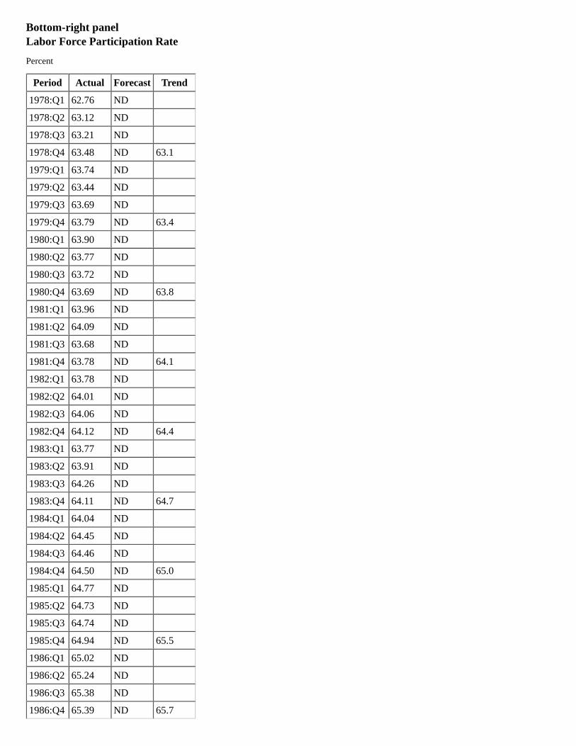
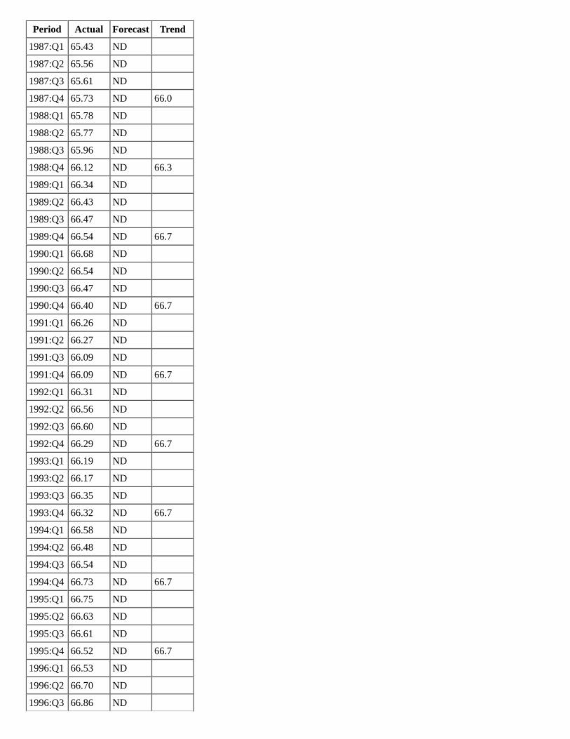
Bottom-right panelLabor Force Participation Rate

Percent

Period Actual Forecast Trend

1978:Q1 62.76 ND

1978:Q2 63.12 ND

1978:Q3 63.21 ND

1978:Q4 63.48 ND 63.1

1979:Q1 63.74 ND

1979:Q2 63.44 ND

1979:Q3 63.69 ND

1979:Q4 63.79 ND 63.4

1980:Q1 63.90 ND

1980:Q2 63.77 ND

1980:Q3 63.72 ND

1980:Q4 63.69 ND 63.8

1981:Q1 63.96 ND

1981:Q2 64.09 ND

1981:Q3 63.68 ND

1981:Q4 63.78 ND 64.1

1982:Q1 63.78 ND

1982:Q2 64.01 ND

1982:Q3 64.06 ND

1982:Q4 64.12 ND 64.4

1983:Q1 63.77 ND

1983:Q2 63.91 ND

1983:Q3 64.26 ND

1983:Q4 64.11 ND 64.7

1984:Q1 64.04 ND

1984:Q2 64.45 ND

1984:Q3 64.46 ND

1984:Q4 64.50 ND 65.0

1985:Q1 64.77 ND

1985:Q2 64.73 ND

1985:Q3 64.74 ND

1985:Q4 64.94 ND 65.5

1986:Q1 65.02 ND

1986:Q2 65.24 ND

1986:Q3 65.38 ND

1986:Q4 65.39 ND 65.7


1987:Q1 65.43 ND

1987:Q2 65.56 ND

1987:Q3 65.61 ND

1987:Q4 65.73 ND 66.0

1988:Q1 65.78 ND

1988:Q2 65.77 ND

1988:Q3 65.96 ND

1988:Q4 66.12 ND 66.3

1989:Q1 66.34 ND

1989:Q2 66.43 ND

1989:Q3 66.47 ND

1989:Q4 66.54 ND 66.7

1990:Q1 66.68 ND

1990:Q2 66.54 ND

1990:Q3 66.47 ND

1990:Q4 66.40 ND 66.7

1991:Q1 66.26 ND

1991:Q2 66.27 ND

1991:Q3 66.09 ND

1991:Q4 66.09 ND 66.7

1992:Q1 66.31 ND

1992:Q2 66.56 ND

1992:Q3 66.60 ND

1992:Q4 66.29 ND 66.7

1993:Q1 66.19 ND

1993:Q2 66.17 ND

1993:Q3 66.35 ND

1993:Q4 66.32 ND 66.7

1994:Q1 66.58 ND

1994:Q2 66.48 ND

1994:Q3 66.54 ND

1994:Q4 66.73 ND 66.7

1995:Q1 66.75 ND

1995:Q2 66.63 ND

1995:Q3 66.61 ND

1995:Q4 66.52 ND 66.7

1996:Q1 66.53 ND

1996:Q2 66.70 ND

1996:Q3 66.86 ND


1996:Q4 67.02 ND 66.7

1997:Q1 66.99 ND

1997:Q2 67.11 ND

1997:Q3 67.16 ND

1997:Q4 67.14 ND 66.7

1998:Q1 67.10 ND

1998:Q2 67.02 ND

1998:Q3 67.07 ND

1998:Q4 67.17 ND 66.7

1999:Q1 67.14 ND

1999:Q2 67.08 ND

1999:Q3 67.05 ND

1999:Q4 67.09 ND 66.7

2000:Q1 67.29 ND

2000:Q2 67.18 ND

2000:Q3 66.90 ND

2000:Q4 66.94 ND 66.7

2001:Q1 67.15 ND

2001:Q2 66.80 ND

2001:Q3 66.69 ND

2001:Q4 66.76 ND 66.7

2002:Q1 66.58 ND

2002:Q2 66.65 ND

2002:Q3 66.65 ND

2002:Q4 66.46 ND 66.7

2003:Q1 66.27 ND

2003:Q2 66.40 ND

2003:Q3 66.19 ND

2003:Q4 ND 66.13 66.7

2004:Q1 ND 66.22

2004:Q2 ND 66.26

2004:Q3 ND 66.35

2004:Q4 ND 66.51 66.7

2005:Q1 ND 66.64

2005:Q2 ND 66.70

2005:Q3 ND 66.78

2005:Q4 ND 66.80 66.7

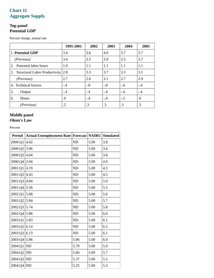
Chart 11Aggregate Supply

Top panelPotential GDP

Percent change, annual rate

1995-2001 2002 2003 2004 2005

1. Potential GDP 3.4 3.6 4.0 3.7 3.7

(Previous) 3.4 3.5 3.9 3.5 3.7

2. Potential labor hours 1.0 1.1 1.1 1.1 1.1

3. Structural Labor Productivity 2.8 3.3 3.7 3.3 3.1

(Previous) 2.7 2.6 3.1 2.7 2.9

4. Technical factors -.4 -.8 -.8 -.6 -.4

5. Output -.4 -.4 -.4 -.4 -.4

6. Hours .0 -.4 -.4 -.2 .0

(Previous) .2 .3 .3 .3 .3

Middle panelOkun's Law

Percent

Period Actual Unemployment Rate Forecast NAIRU Simulated

2000:Q1 4.02 ND 5.00 3.8

2000:Q2 3.96 ND 5.00 3.6

2000:Q3 4.04 ND 5.00 3.8

2000:Q4 3.94 ND 5.00 4.0

2001:Q1 4.19 ND 5.00 4.3

2001:Q2 4.43 ND 5.00 4.5

2001:Q3 4.84 ND 5.00 5.0

2001:Q4 5.58 ND 5.00 5.5

2002:Q1 5.68 ND 5.00 5.6

2002:Q2 5.84 ND 5.00 5.7

2002:Q3 5.74 ND 5.00 5.8

2002:Q4 5.88 ND 5.00 6.0

2003:Q1 5.83 ND 5.00 6.1

2003:Q2 6.14 ND 5.00 6.3

2003:Q3 6.13 ND 5.00 6.1

2003:Q4 5.86 5.86 5.00 6.0

2004:Q1 ND 5.79 5.00 5.9

2004:Q2 ND 5.60 5.00 5.7

2004:Q3 ND 5.37 5.00 5.5

2004:Q4 ND 5.25 5.00 5.3

Period Actual Unemployment Rate Forecast NAIRU Simulated

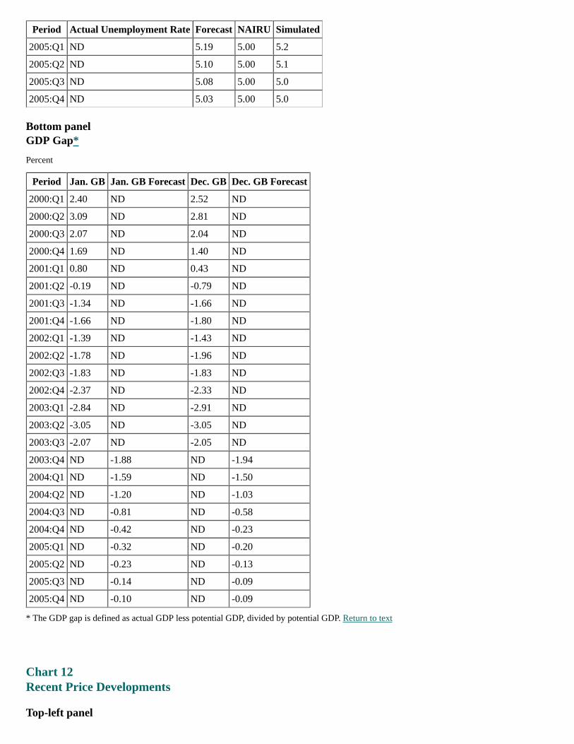
2005:Q1 ND 5.19 5.00 5.2

2005:Q2 ND 5.10 5.00 5.1

2005:Q3 ND 5.08 5.00 5.0

2005:Q4 ND 5.03 5.00 5.0

Bottom panelGDP Gap*

Percent

Period Jan. GB Jan. GB Forecast Dec. GB Dec. GB Forecast

2000:Q1 2.40 ND 2.52 ND

2000:Q2 3.09 ND 2.81 ND

2000:Q3 2.07 ND 2.04 ND

2000:Q4 1.69 ND 1.40 ND

2001:Q1 0.80 ND 0.43 ND

2001:Q2 -0.19 ND -0.79 ND

2001:Q3 -1.34 ND -1.66 ND

2001:Q4 -1.66 ND -1.80 ND

2002:Q1 -1.39 ND -1.43 ND

2002:Q2 -1.78 ND -1.96 ND

2002:Q3 -1.83 ND -1.83 ND

2002:Q4 -2.37 ND -2.33 ND

2003:Q1 -2.84 ND -2.91 ND

2003:Q2 -3.05 ND -3.05 ND

2003:Q3 -2.07 ND -2.05 ND

2003:Q4 ND -1.88 ND -1.94

2004:Q1 ND -1.59 ND -1.50

2004:Q2 ND -1.20 ND -1.03

2004:Q3 ND -0.81 ND -0.58

2004:Q4 ND -0.42 ND -0.23

2005:Q1 ND -0.32 ND -0.20

2005:Q2 ND -0.23 ND -0.13

2005:Q3 ND -0.14 ND -0.09

2005:Q4 ND -0.10 ND -0.09

* The GDP gap is defined as actual GDP less potential GDP, divided by potential GDP. Return to text

Chart 12Recent Price Developments

Top-left panel

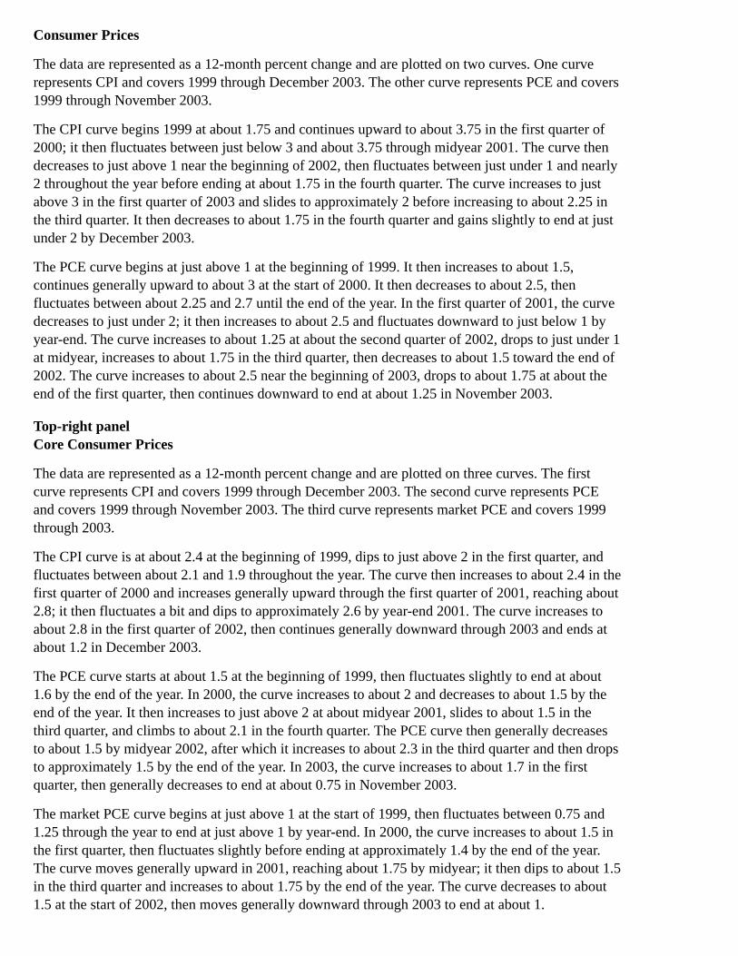
Consumer Prices

The data are represented as a 12-month percent change and are plotted on two curves. One curverepresents CPI and covers 1999 through December 2003. The other curve represents PCE and covers1999 through November 2003.

The CPI curve begins 1999 at about 1.75 and continues upward to about 3.75 in the first quarter of2000; it then fluctuates between just below 3 and about 3.75 through midyear 2001. The curve thendecreases to just above 1 near the beginning of 2002, then fluctuates between just under 1 and nearly2 throughout the year before ending at about 1.75 in the fourth quarter. The curve increases to justabove 3 in the first quarter of 2003 and slides to approximately 2 before increasing to about 2.25 inthe third quarter. It then decreases to about 1.75 in the fourth quarter and gains slightly to end at justunder 2 by December 2003.

The PCE curve begins at just above 1 at the beginning of 1999. It then increases to about 1.5,continues generally upward to about 3 at the start of 2000. It then decreases to about 2.5, thenfluctuates between about 2.25 and 2.7 until the end of the year. In the first quarter of 2001, the curvedecreases to just under 2; it then increases to about 2.5 and fluctuates downward to just below 1 byyear-end. The curve increases to about 1.25 at about the second quarter of 2002, drops to just under 1at midyear, increases to about 1.75 in the third quarter, then decreases to about 1.5 toward the end of2002. The curve increases to about 2.5 near the beginning of 2003, drops to about 1.75 at about theend of the first quarter, then continues downward to end at about 1.25 in November 2003.

Top-right panelCore Consumer Prices

The data are represented as a 12-month percent change and are plotted on three curves. The firstcurve represents CPI and covers 1999 through December 2003. The second curve represents PCEand covers 1999 through November 2003. The third curve represents market PCE and covers 1999through 2003.

The CPI curve is at about 2.4 at the beginning of 1999, dips to just above 2 in the first quarter, andfluctuates between about 2.1 and 1.9 throughout the year. The curve then increases to about 2.4 in thefirst quarter of 2000 and increases generally upward through the first quarter of 2001, reaching about2.8; it then fluctuates a bit and dips to approximately 2.6 by year-end 2001. The curve increases toabout 2.8 in the first quarter of 2002, then continues generally downward through 2003 and ends atabout 1.2 in December 2003.

The PCE curve starts at about 1.5 at the beginning of 1999, then fluctuates slightly to end at about1.6 by the end of the year. In 2000, the curve increases to about 2 and decreases to about 1.5 by theend of the year. It then increases to just above 2 at about midyear 2001, slides to about 1.5 in thethird quarter, and climbs to about 2.1 in the fourth quarter. The PCE curve then generally decreasesto about 1.5 by midyear 2002, after which it increases to about 2.3 in the third quarter and then dropsto approximately 1.5 by the end of the year. In 2003, the curve increases to about 1.7 in the firstquarter, then generally decreases to end at about 0.75 in November 2003.

The market PCE curve begins at just above 1 at the start of 1999, then fluctuates between 0.75 and1.25 through the year to end at just above 1 by year-end. In 2000, the curve increases to about 1.5 inthe first quarter, then fluctuates slightly before ending at approximately 1.4 by the end of the year.The curve moves generally upward in 2001, reaching about 1.75 by midyear; it then dips to about 1.5in the third quarter and increases to about 1.75 by the end of the year. The curve decreases to about1.5 at the start of 2002, then moves generally downward through 2003 to end at about 1.

Middle-left panelCPI Food Prices

Period Percent change, annual rate

2000 2.48

2001 3.19

2002 1.20

2003:Q1 2.00

2003:Q2 2.50

2003:Q3 2.90

2003:Q4 5.40

Middle-right panelLive Cattle Prices

The period covered is August 2003 through January 26, 2004. The data are represented as dollars perhundred pounds and are plotted on two curves. The first curve represents spot, and the second curverepresents futures five months ahead. A vertical line, drawn toward the end of December 2003,indicates when mad cow disease was discovered in the United States.

The spot curve starts just below 80 dollars in August 2003 and fluctuates between about 79 dollarsand 80 dollars through the end of the month. In September, the curve increases to about 85 dollars inthe first half of the month and remains at about that level until month-end. The curve climbs to about110 dollars in mid-October and drops to about 92 dollars by the end of the month. In November, thecurve increases to about 102 dollars in the first quarter of the month, dips to about 99 dollars atmid-month, and increases to about 100 dollars by month-end. It then decreases to about 75 dollarstoward the end of December and stays at about that level through the beginning of January. The spotcurve then increases to about 82 dollars by January 26, 2004.

The futures curve begins in August 2003 at about 79 dollars and fluctuates between about 79 dollarsand 82 dollars through the third quarter of November. The curve then drops to about 78 dollars at theend of November and fluctuates downward in December, reaching about 70 dollars by month-end.The curve moves upward in January, ending at about 72 dollars on January 26, 2004.

Bottom-left panelLabor Costs

The figure shows labor costs for production or nonsupervisory workers. The data are represented as a12-month percent change and are plotted on two curves. The first curve represents average hourlyearnings and covers 2000 through December 2003. The second curve represents ECI wages andsalaries and covers 2000 through September 2003.

The average hourly earnings curve starts just above 3.5 in 2000 and fluctuates between 3.6 and 3.7through the fourth quarter, then increases to about 4.4 by year-end. It then decreases to about 3.9 atthe start of 2001. The curve fluctuates downward to just above 2.5 in the first half of 2002, increasesto about 3.0 in the third quarter, and fluctuates between about 2.9 and 3.1 for the remainder of theyear. In 2003, the curve increases to about 3.5 at the beginning of the year, then generally continuesdownward to end at about 2.0 in December 2003.

The ECI wages and salaries curve begins at about 3.9 in 2000 and increases to about 4.0 in the thirdquarter. The curve then decreases to about 3.6 in mid-2001 and increases to about 3.7 by year-end.

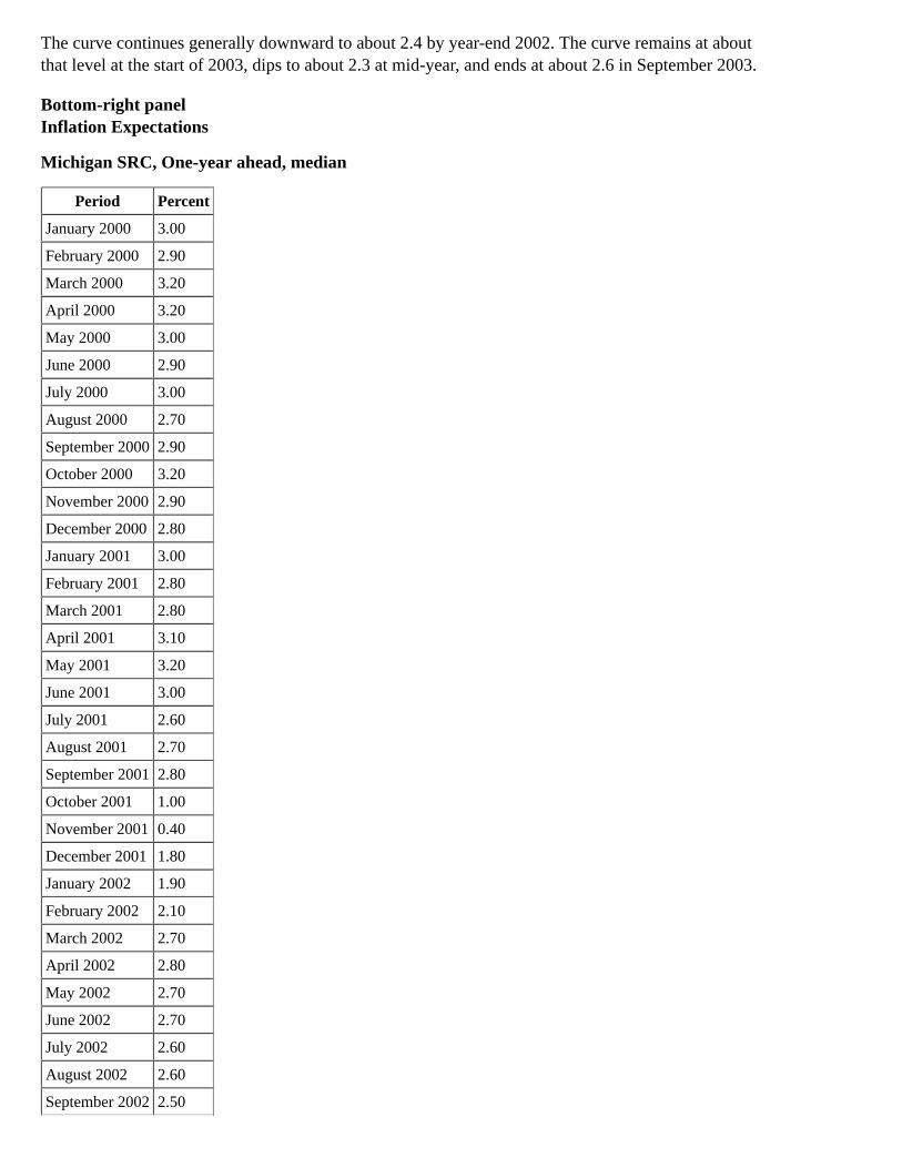
The curve continues generally downward to about 2.4 by year-end 2002. The curve remains at aboutthat level at the start of 2003, dips to about 2.3 at mid-year, and ends at about 2.6 in September 2003.

Bottom-right panelInflation Expectations

Michigan SRC, One-year ahead, median

Period Percent

January 2000 3.00

February 2000 2.90

March 2000 3.20

April 2000 3.20

May 2000 3.00

June 2000 2.90

July 2000 3.00

August 2000 2.70

September 2000 2.90

October 2000 3.20

November 2000 2.90

December 2000 2.80

January 2001 3.00

February 2001 2.80

March 2001 2.80

April 2001 3.10

May 2001 3.20

June 2001 3.00

July 2001 2.60

August 2001 2.70

September 2001 2.80

October 2001 1.00

November 2001 0.40

December 2001 1.80

January 2002 1.90

February 2002 2.10

March 2002 2.70

April 2002 2.80

May 2002 2.70

June 2002 2.70

July 2002 2.60

August 2002 2.60

September 2002 2.50

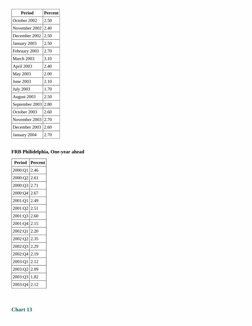
Period Percent

October 2002 2.50

November 2002 2.40

December 2002 2.50

January 2003 2.50

February 2003 2.70

March 2003 3.10

April 2003 2.40

May 2003 2.00

June 2003 2.10

July 2003 1.70

August 2003 2.50

September 2003 2.80

October 2003 2.60

November 2003 2.70

December 2003 2.60

January 2004 2.70

FRB Philidelphia, One-year ahead

Period Percent

2000:Q1 2.46

2000:Q2 2.61

2000:Q3 2.71

2000:Q4 2.67

2001:Q1 2.49

2001:Q2 2.51

2001:Q3 2.60

2001:Q4 2.15

2002:Q1 2.20

2002:Q2 2.35

2002:Q3 2.29

2002:Q4 2.19

2003:Q1 2.12

2003:Q2 2.09

2003:Q3 1.82

2003:Q4 2.12

Chart 13

Inflation Outlook

Top-left panelPCE Prices

Period Percent change, Q4/Q4 Forecast

2002 1.83 ND

2003 1.70 ND

2004 ND 1.00

2005 ND 1.00

Top-right panelCore PCE Prices

Period Percent change, Q4/Q4 Forecast

2002 1.58 ND

2003 0.80 ND

2004 ND 1.00

2005 ND 1.00

Middle-left panelCore Non-oil Import Prices

Period Four-quarter percent change Forecast

2002:Q1 -4.09 ND

2002:Q2 -2.38 ND

2002:Q3 -0.65 ND

2002:Q4 0.47 ND

2003:Q1 2.38 ND

2003:Q2 1.82 ND

2003:Q3 1.66 ND

2003:Q4 ND 1.77

2004:Q1 ND 1.38

2004:Q2 ND 2.37

2004:Q3 ND 3.06

2004:Q4 ND 3.26

2005:Q1 ND 2.50

2005:Q2 ND 1.77

2005:Q3 ND 1.08

2005:Q4 ND 0.69

Middle-right panelECI Compensation per Hour

Percent change, annual rate*

PeriodContributionsfrom Benefits

Contributions fromBenefits: Forecast

Contributions fromWages and Salaries

Contributions fromWages and Salaries:

Forecast

2002:H1 1.34 ND 2.67 ND

2002:H2 1.32 ND 1.68 ND

2003:H1 2.15 ND 2.29 ND

2003:H2 1.59 ND 2.11 ND

2004:H1 ND 1.64 ND 1.87

2004:H2 ND 1.71 ND 2.01

2005:H1 ND 1.76 ND 2.00

2005:H2 ND 1.81 ND 2.00

* Half years are Q2/Q4 or Q4/Q2. Return to text

Bottom-left panel

Effective Deflation Core PCE Inflation less than ½ percent

Pernicious Deflation Core PCE Inflation less than ½ percentANDthe unemployment rate above 6 percent

Bottom-right panelProbability of Deflation

Percent

Effective DeflationPerniciousDeflation

Jan. 2003 24 10

June 2003 30 10

Jan. 2004 22 5

Chart 14

Top panelECONOMIC PROJECTIONS FOR 2004

FOMC

StaffRange

CentralTendency

Percentage change, Q4 to Q4

Nominal GDP 5½ to 6½ 5½ to 6¼ 6.2

(June 2003) (4¾ to 6½) (5¼ to 6¼)

Real GDP 4 to 5½ 4½ to 5 5.3

(June 2003) (3½ to 5¼) (3¾ to 4¾)

PCE Prices 1 to 1½ 1 to 1¼ 1.0

FOMC

StaffRange

CentralTendency

(June 2003) (¾ to 2) (1 to 1½)

Average level, Q4, percent

Unemployment rate 5¼ to 5½ 5¼ to 5½ 5.3

(June 2003) (5½ to 6¼) (5½ to 6)

Central tendencies calculated by dropping high and low three from ranges.

Appendix 6: Materials used by Mr. Reinhart

Material for Briefing on Monetary Policy AlternativesJanuary 28, 2004

STRICTLY CONFIDENTIAL (FR)CLASS I FOMC

Exhibit 1

Top-left panelExpected Federal Funds Rates*

A line chart displays the expected path of the federal funds rate embedded in futures quotes as ofDecember 8, 2003 and January 27, 2004. The chart indicates a downward revision of the expectedpath of the federal funds rate over the intermeeting period. The most recent futures quotes suggestthat the federal funds rate will rise to around 3.25 percent by the first quarter of 2006.

* Estimates from federal funds and eurodollar futures, with an allowance for term premia and other adjustments. Return to text

Top-right panelProbability Distribution of Time to the Beginning of Tightening

A line chart shows a probability distribution of the time to the beginning of tightening of monetarypolicy as of December 8, 2003 and January 27, 2004. The distribution shifted to the right during theintermeeting period and suggests that expectations for the onset of policy tightening have shifted outfive months into the future, from five months on average to nearly ten months.

Middle-left panelImplied Distribution of Federal Funds Rate About 6 Months Ahead*

A bar graph shows the implied distribution of the federal funds rate six-months ahead as ofDecember 8, 2003 and January 27, 2004. Over the intermeeting period the weight of this distributionshifted to the left slightly, with greater probability attached to a federal funds rate in theneighborhood of ¾ to 1 percent and less probability associated with federal funds rates in theneighborhood of 1½ to 2¼ percent.

* Based on the distribution of the three-month eurodollar rate five months ahead (adjusted for a risk premium), as implied byoptions on eurodollar futures contracts. Return to text

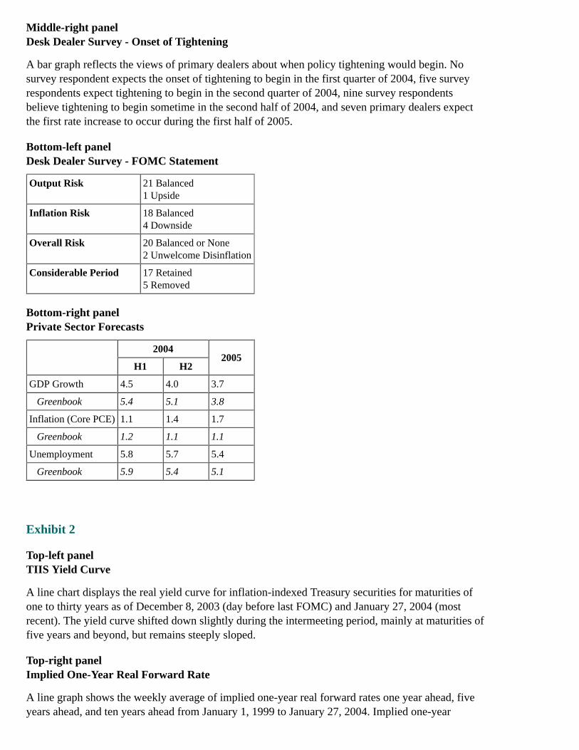
Middle-right panelDesk Dealer Survey - Onset of Tightening

A bar graph reflects the views of primary dealers about when policy tightening would begin. Nosurvey respondent expects the onset of tightening to begin in the first quarter of 2004, five surveyrespondents expect tightening to begin in the second quarter of 2004, nine survey respondentsbelieve tightening to begin sometime in the second half of 2004, and seven primary dealers expectthe first rate increase to occur during the first half of 2005.

Bottom-left panelDesk Dealer Survey - FOMC Statement

Output Risk 21 Balanced1 Upside

Inflation Risk 18 Balanced4 Downside

Overall Risk 20 Balanced or None2 Unwelcome Disinflation

Considerable Period 17 Retained5 Removed

Bottom-right panelPrivate Sector Forecasts

2004

2005H1 H2

GDP Growth 4.5 4.0 3.7

Greenbook 5.4 5.1 3.8

Inflation (Core PCE) 1.1 1.4 1.7


Unemployment 5.8 5.7 5.4


Exhibit 2

Top-left panelTIIS Yield Curve

A line chart displays the real yield curve for inflation-indexed Treasury securities for maturities ofone to thirty years as of December 8, 2003 (day before last FOMC) and January 27, 2004 (mostrecent). The yield curve shifted down slightly during the intermeeting period, mainly at maturities offive years and beyond, but remains steeply sloped.

Top-right panelImplied One-Year Real Forward Rate

A line graph shows the weekly average of implied one-year real forward rates one year ahead, fiveyears ahead, and ten years ahead from January 1, 1999 to January 27, 2004. Implied one-year

forward rates have continued to fall, consistent with recent trends, with the one-year forward rate oneyear ahead falling further than those at longer maturities.

Middle-left panelThe Case for Easier Policy

Business confidence may remain impaired.Inflation is low and poised to go lower.

Middle-right panelThe Case for Firmer Policy

Considerable financial accomodation is in place.Inflation pressures may emerge more quickly than in the staff forecast.

Bottom-left panelSelected Money and Credit Aggregates

2003 2004

H1 Q3 Q4 Jan.

M2 7.7 7.0 -1.8 -1.5

Bank Credit -9.7 4.6 -0.5 2.2

Business Loans -6.4 -13.9 -9.7 -7.4

Bottom-right panelChange in Selected Financial Market Conditions Since Last FOMC

BasisPoints

Ten-Year Treasury -20

A Corporate -22

Percent

Wilshire 7.2

Major Currency Index -1.7

Exhibit 3Alternative Strategies for Removing Policy Accomodation

Top-left panelCase for Keeping Policy on Hold

Long-term inflation expectations seem well-anchored.Simulations suggest that policy can remain on hold for an extended period without fuelingstrong inflation pressures.

Top-right panelInflation Expectations

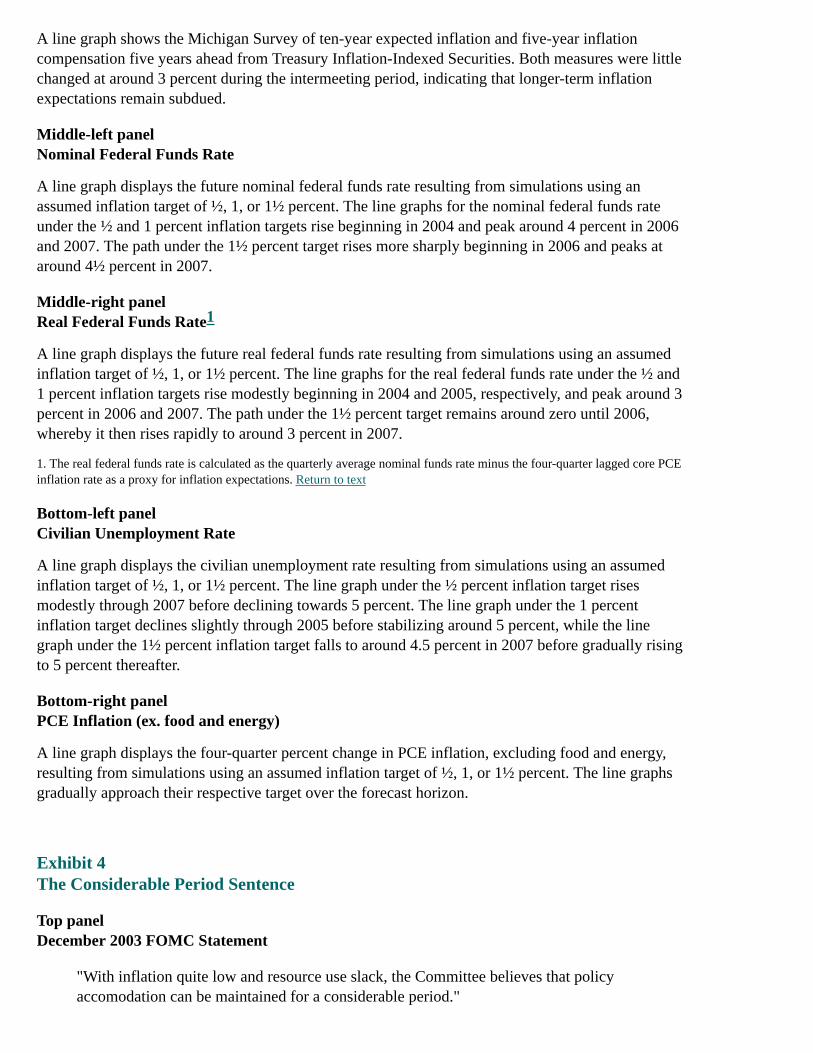
A line graph shows the Michigan Survey of ten-year expected inflation and five-year inflationcompensation five years ahead from Treasury Inflation-Indexed Securities. Both measures were littlechanged at around 3 percent during the intermeeting period, indicating that longer-term inflationexpectations remain subdued.

Middle-left panelNominal Federal Funds Rate

A line graph displays the future nominal federal funds rate resulting from simulations using anassumed inflation target of ½, 1, or 1½ percent. The line graphs for the nominal federal funds rateunder the ½ and 1 percent inflation targets rise beginning in 2004 and peak around 4 percent in 2006and 2007. The path under the 1½ percent target rises more sharply beginning in 2006 and peaks ataround 4½ percent in 2007.

Middle-right panelReal Federal Funds Rate

A line graph displays the future real federal funds rate resulting from simulations using an assumedinflation target of ½, 1, or 1½ percent. The line graphs for the real federal funds rate under the ½ and1 percent inflation targets rise modestly beginning in 2004 and 2005, respectively, and peak around 3percent in 2006 and 2007. The path under the 1½ percent target remains around zero until 2006,whereby it then rises rapidly to around 3 percent in 2007.

1. The real federal funds rate is calculated as the quarterly average nominal funds rate minus the four-quarter lagged core PCEinflation rate as a proxy for inflation expectations. Return to text

Bottom-left panelCivilian Unemployment Rate

A line graph displays the civilian unemployment rate resulting from simulations using an assumedinflation target of ½, 1, or 1½ percent. The line graph under the ½ percent inflation target risesmodestly through 2007 before declining towards 5 percent. The line graph under the 1 percentinflation target declines slightly through 2005 before stabilizing around 5 percent, while the linegraph under the 1½ percent inflation target falls to around 4.5 percent in 2007 before gradually risingto 5 percent thereafter.

Bottom-right panelPCE Inflation (ex. food and energy)

A line graph displays the four-quarter percent change in PCE inflation, excluding food and energy,resulting from simulations using an assumed inflation target of ½, 1, or 1½ percent. The line graphsgradually approach their respective target over the forecast horizon.

Exhibit 4The Considerable Period Sentence

Top panelDecember 2003 FOMC Statement

"With inflation quite low and resource use slack, the Committee believes that policyaccomodation can be maintained for a considerable period."

1

Middle panelsConsiderable Period Options

Middle-left panelRetain

Confident economy will evolve in a benign manner.Or inflation on low side of desired range.

Middle-center panelDrop

Tightening within next few meetings not ruled out.Costs of having to delay tightening or renege damaging.

Middle-right panelModify

Outsized market reaction to dropping."Patience" would imply gradual firming.

Bottom panelPotential Alternative

"With inflation quite low and resource use slack, the Committee believes that it can bepatient in removing its policy accomodation."

Return to top

Home | Monetary policy | FOMC | FOMC transcriptsAccessibility | Contact UsLast update: April 30, 2010

Documents

Fomc 20040128 Text Material