Embed Size (px)
Citation preview
FLOLAB – FLAT PLATE
Anoop SamantYanyan ZhangSaptarshi Basu
Andres Chaparro
INTRODUCTION
Model the laminar and turbulent flow over a flat plate
Compare with the theoretical predictions
Study of flow parameters like Nusselt Number, Skin Friction Coefficient, shear layer thickness, velocity and temperature
Effects of change in length and initial flow conditions
THEORY
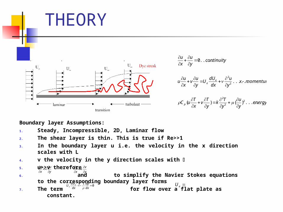
Boundary layer Assumptions: 1. Steady, Incompressible, 2D, Laminar flow2. The shear layer is thin. This is true if Re>>13. In the boundary layer u i.e. the velocity in the x direction scales
with L4. v the velocity in the y direction scales with 5. u>>v therefore 6. and to simplify the Navier Stokes equations to the
corresponding boundary layer forms7. The term for flow over a flat plate as
constant.
energyy
u
y
Tk
y
Tv
x
TuC
momentumxy
u
dx
dUU
y
uv
x
uu
continuityy
u
x
u
p
ee
.......)()(
......
.....0
22
2
2
2
y
u
x
u
y
v
x
v
01
dx
dp
dx
dUU ee
eU
THEORY
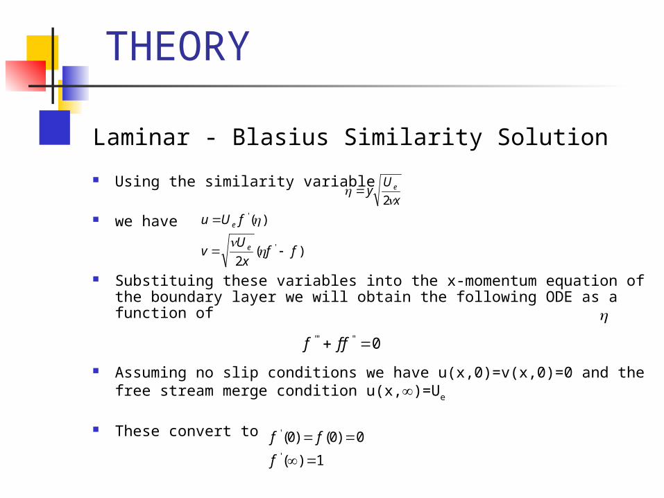
Laminar - Blasius Similarity Solution
Using the similarity variable
we have
Substituing these variables into the x-momentum equation of the boundary layer we will obtain the following ODE as a function of
Assuming no slip conditions we have u(x,0)=v(x,0)=0 and the free stream merge condition u(x,)=Ue
These convert to
x
Uy e
2
)(2
)(
'
'
ffx
Uv
fUu
e
e
0''''' fff
1)(
0)0()0('
'
f
ff
THEORY
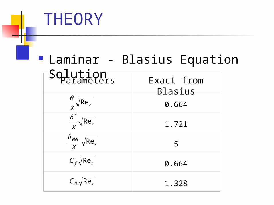
Laminar - Blasius Equation Solution
xxRe
xxRe
*
xxRe%99
xfC Re
xDC Re
Parameters Exact from Blasius
0.664
1.721
5
0.664
1.328
THEORY
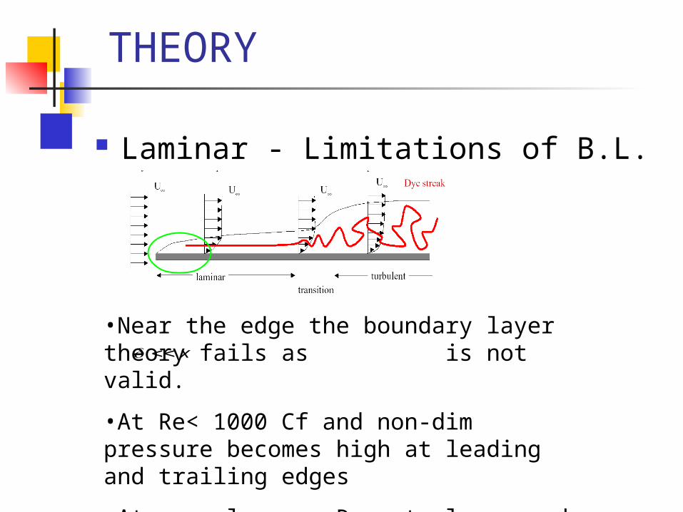
Laminar - Limitations of B.L.
•Near the edge the boundary layer theory fails as is not valid.
•At Re< 1000 Cf and non-dim pressure becomes high at leading and trailing edges
•At very large x Re gets large and the flow gets separated.
x
THEORY
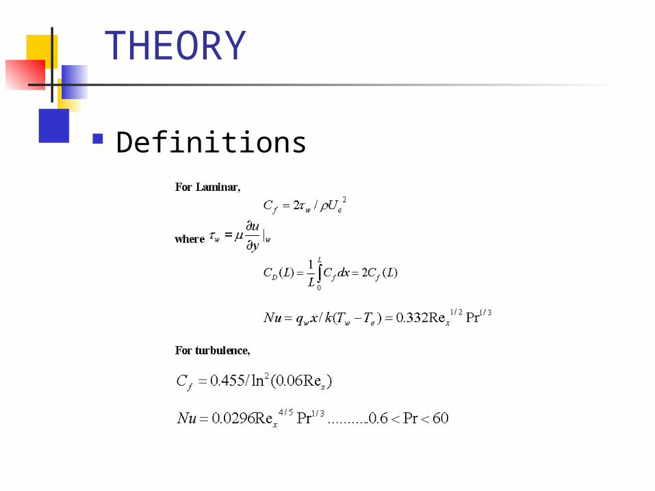
Definitions
THEORY
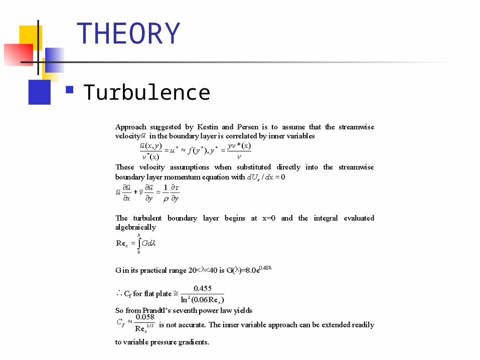
Turbulence
Flolab Parameters
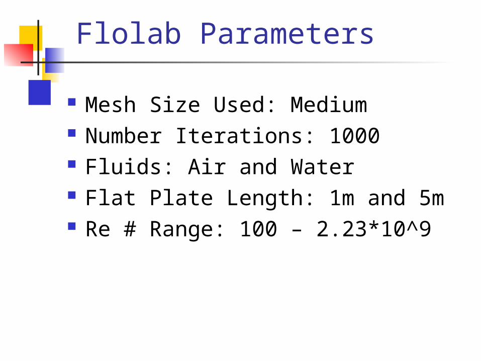
Mesh Size Used: Medium Number Iterations: 1000 Fluids: Air and Water Flat Plate Length: 1m and 5m Re # Range: 100 – 2.23*10^9
RESULTS – Velocity Profiles
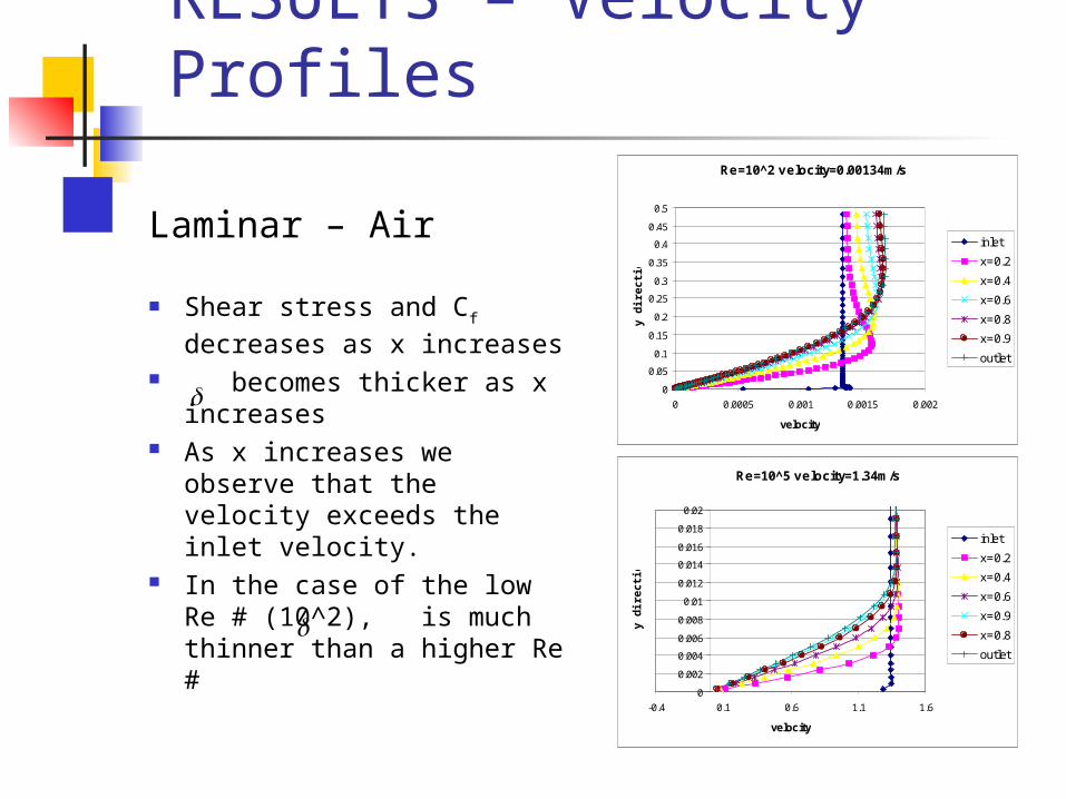
Laminar – Air
Shear stress and Cf decreases as x increases
becomes thicker as x increases
As x increases we observe that the velocity exceeds the inlet velocity.
In the case of the low Re # (10^2), is much thinner than a higher Re #
Re=10^5 velocity=1.34m/s
0
0.002
0.004
0.006
0.008
0.01
0.012
0.014
0.016
0.018
0.02
-0.4 0.1 0.6 1.1 1.6
velocity
y d
ire
cti
on
inlet
x=0.2
x=0.4
x=0.6
x=0.9
x=0.8
outlet
Re=10^2 velocity=0.00134m/s
0
0.05
0.1
0.15
0.2
0.25
0.3
0.35
0.4
0.45
0.5
0 0.0005 0.001 0.0015 0.002
velocity
y d
ire
cti
on
inlet
x=0.2
x=0.4
x=0.6
x=0.8
x=0.9
outlet
RESULTS – Velocity Profiles
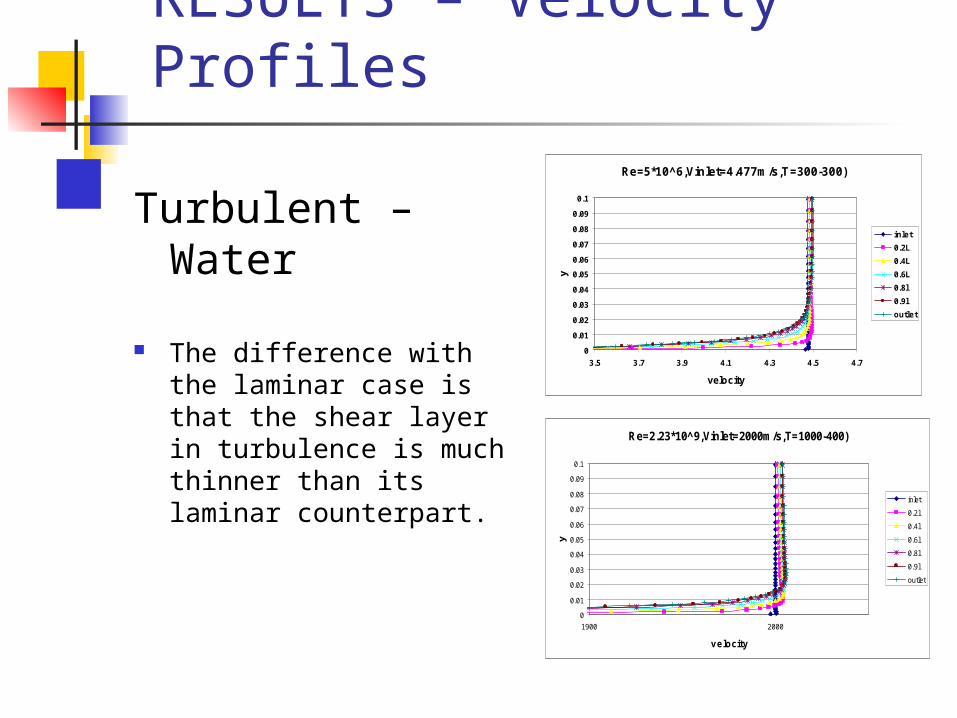
Turbulent – Water
The difference with the laminar case is that the shear layer in turbulence is much thinner than its laminar counterpart.
Re=5*10^6,Vinlet=4.477m/s,T=300-300)
0
0.01
0.02
0.03
0.04
0.05
0.06
0.07
0.08
0.09
0.1
3.5 3.7 3.9 4.1 4.3 4.5 4.7
velocity
y
inlet
0.2L
0.4L
0.6L
0.8l
0.9l
outlet
Re=2.23*10^9,Vinlet=2000m/s,T=1000-400)
0
0.01
0.02
0.03
0.04
0.05
0.06
0.07
0.08
0.09
0.1
1900 2000
ve locity
y
inlet
0.2l
0.4l
0.6l
0.8l
0.9l
outlet
RESULTS – Skin Friction (Cf)
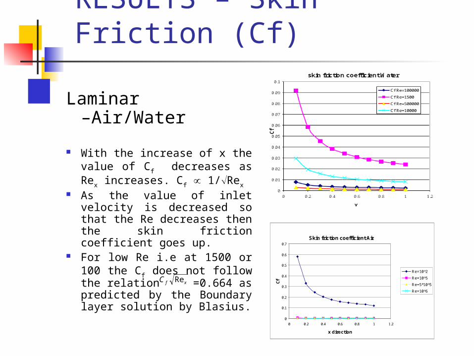
Laminar –Air/Water
With the increase of x the value of Cf decreases as Rex increases. Cf 1/Rex
As the value of inlet velocity is decreased so that the Re decreases then the skin friction coefficient goes up.
For low Re i.e at 1500 or 100 the Cf does not follow the relation =0.664 as predicted by the Boundary layer solution by Blasius.
Skin friction coefficient Air
0
0.1
0.2
0.3
0.4
0.5
0.6
0.7
0 0.2 0.4 0.6 0.8 1 1.2
x direction
Cf
Re=10^2
Re=10^5
Re=5*10^5
Re=10^6
xfC Re
RESULTS – Skin Friction (Cf)
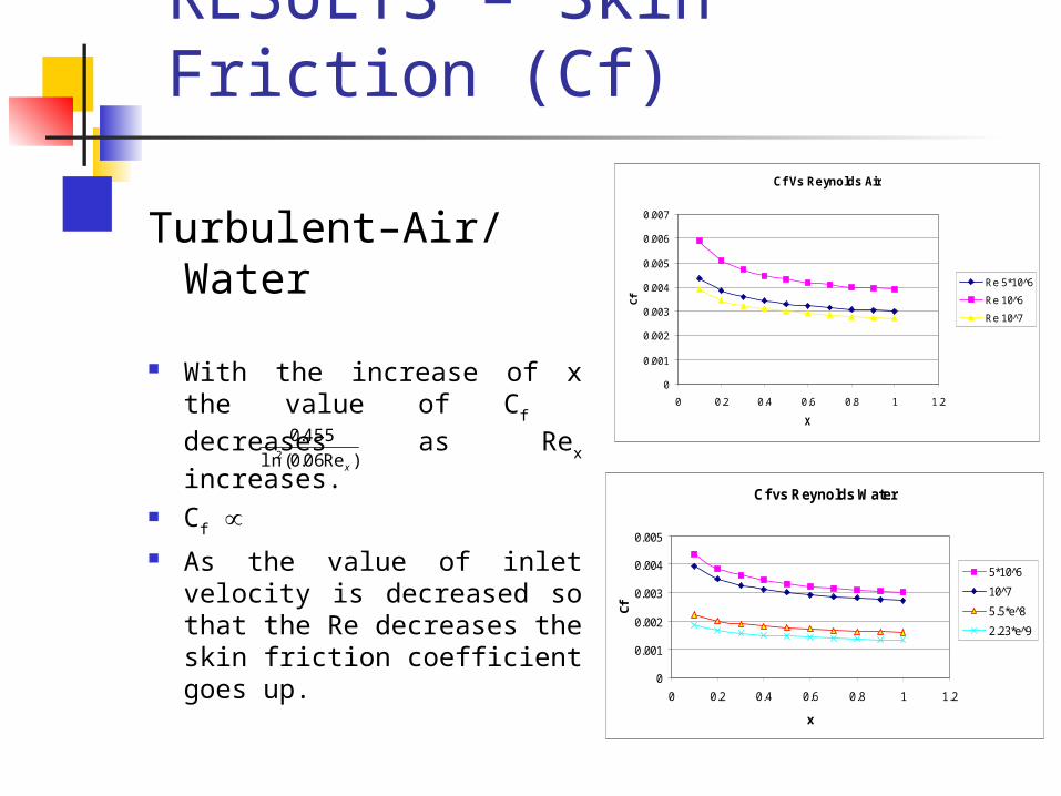
Turbulent–Air/Water
With the increase of x the value of Cf decreases as Rex increases.
Cf As the value of inlet
velocity is decreased so that the Re decreases the skin friction coefficient goes up.
Cf Vs Reynolds Air
0
0.001
0.002
0.003
0.004
0.005
0.006
0.007
0 0.2 0.4 0.6 0.8 1 1.2
X
Cf
Re 5*10^6
Re 10^6
Re 10^7
Cf vs Reynolds Water
0
0.001
0.002
0.003
0.004
0.005
0 0.2 0.4 0.6 0.8 1 1.2
x
Cf
5*10 6̂
10 7̂
5.5*e 8̂
2.23*e 9̂
)Re06.0(ln
455.02
x
RESULTS – Skin Friction (Cf)
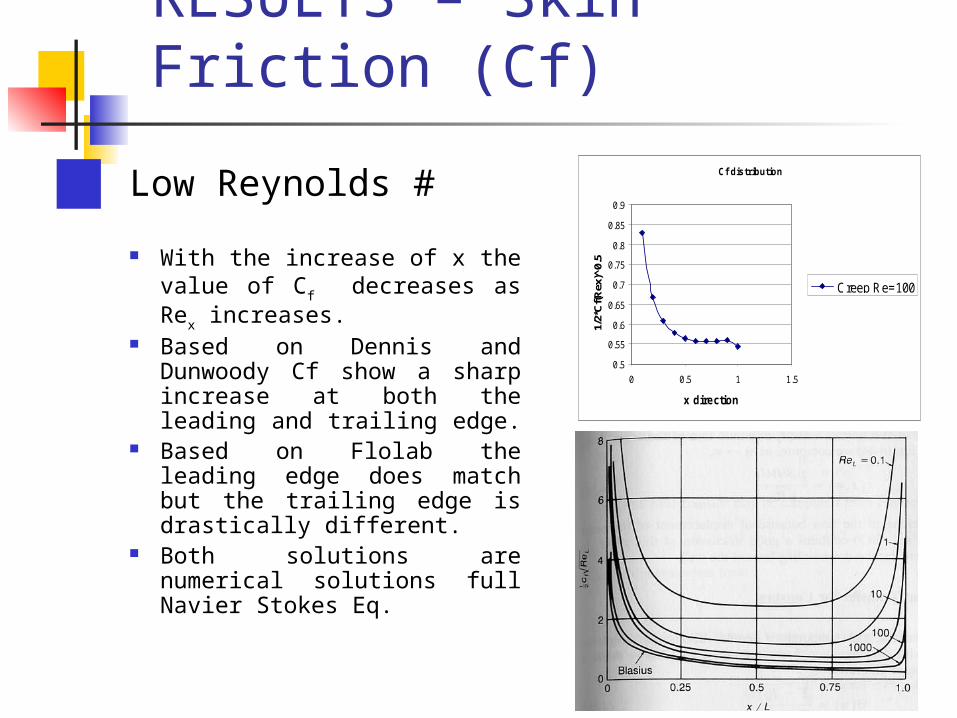
Low Reynolds #
With the increase of x the value of Cf decreases as Rex increases.
Based on Dennis and Dunwoody Cf show a sharp increase at both the leading and trailing edge.
Based on Flolab the leading edge does match but the trailing edge is drastically different.
Both solutions are numerical solutions full Navier Stokes Eq.
Cf distribution
0.5
0.55
0.6
0.65
0.7
0.75
0.8
0.85
0.9
0 0.5 1 1.5
x direction
1/2*
Cf(R
ex)^
0.5
Creep Re=100
RESULTS – Reynolds Similarity
Laminar –Air/Water
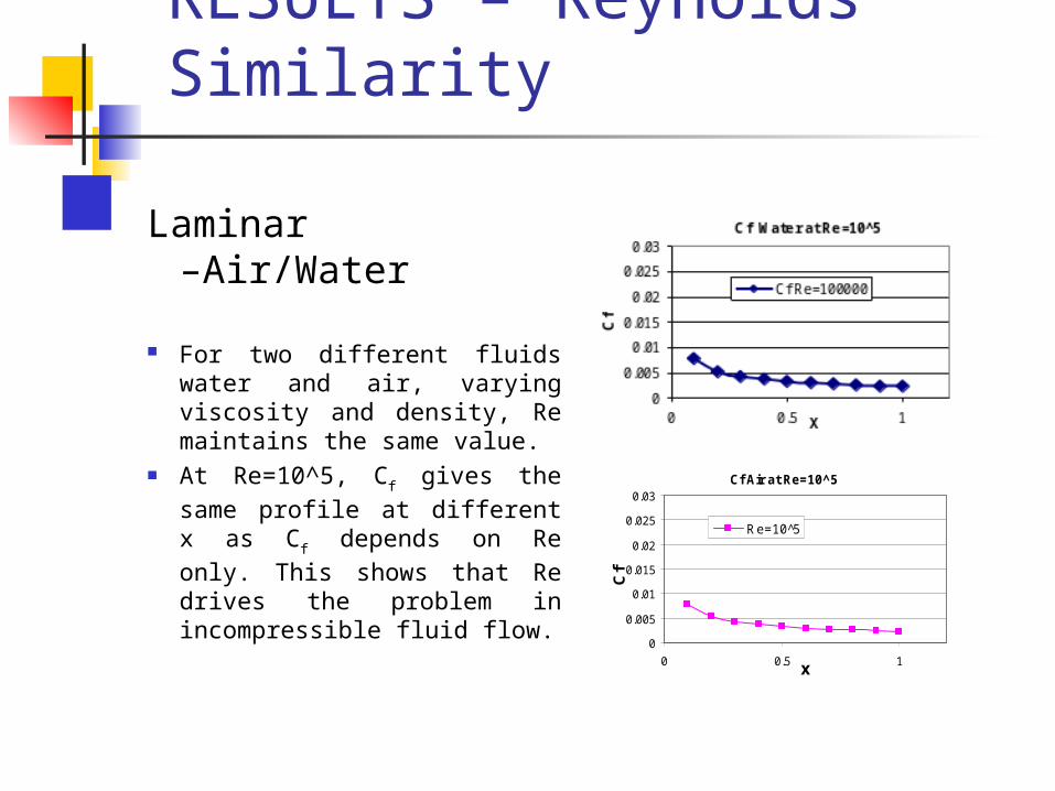
For two different fluids water and air, varying viscosity and density, Re maintains the same value.
At Re=10^5, Cf gives the same profile at different x as Cf depends on Re only. This shows that Re drives the problem in incompressible fluid flow.
Cf Air at Re=10^5
0
0.005
0.01
0.015
0.02
0.025
0.03
0 0.5 1x
Cf
Re=10^5
RESULTS – Skin Friction (Cf)
Laminar – Air
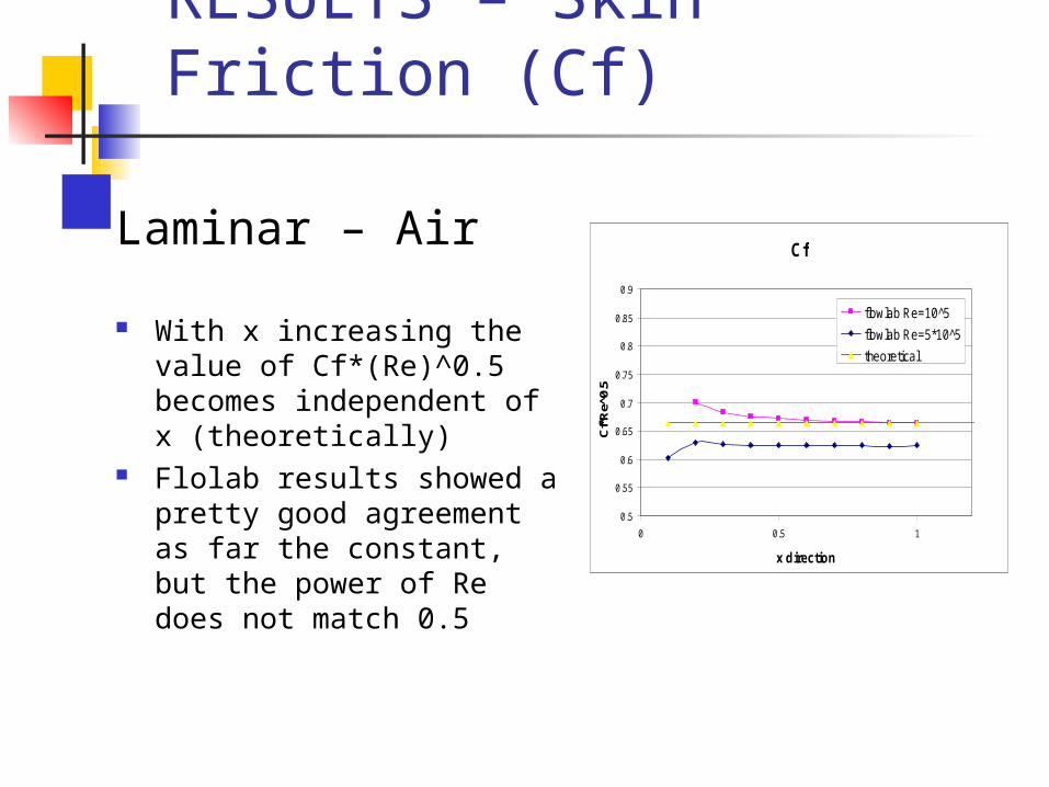
With x increasing the value of Cf*(Re)^0.5 becomes independent of x (theoretically)
Flolab results showed a pretty good agreement as far the constant, but the power of Re does not match 0.5
Cf
0.5
0.55
0.6
0.65
0.7
0.75
0.8
0.85
0.9
0 0.5 1
x direction
Cf*
Re^
0.5
flowlab Re=10^5
flowlab Re=5*10^5
theoretical
RESULTS – Skin Friction (Cf)
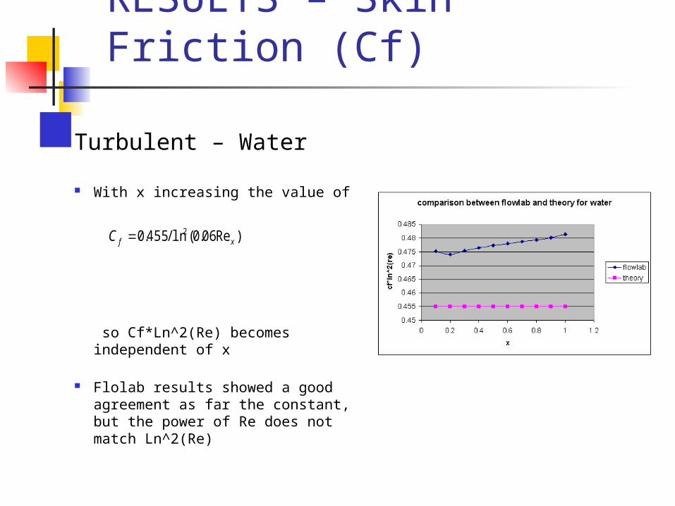
Turbulent – Water
With x increasing the value of
so Cf*Ln^2(Re) becomes independent of x
Flolab results showed a good agreement as far the constant, but the power of Re does not match Ln^2(Re)
)Re06.0(ln/455.0 2xfC
RESULTS – Nusselt Number
Laminar –Water
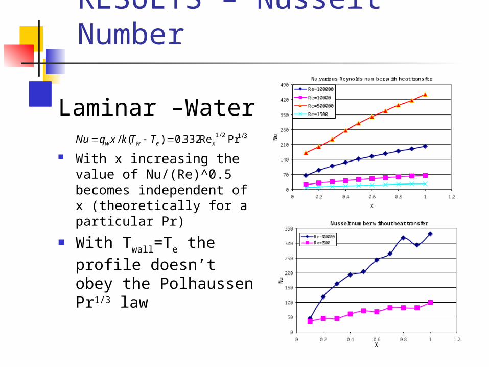
With x increasing the value of Nu/(Re)^0.5 becomes independent of x (theoretically for a particular Pr)
With Twall=Te the profile doesn’t obey the Polhaussen Pr1/3 law
3/12/1 PrRe332.0)(/ xeww TTkxqNu
RESULTS – Nusselt Number
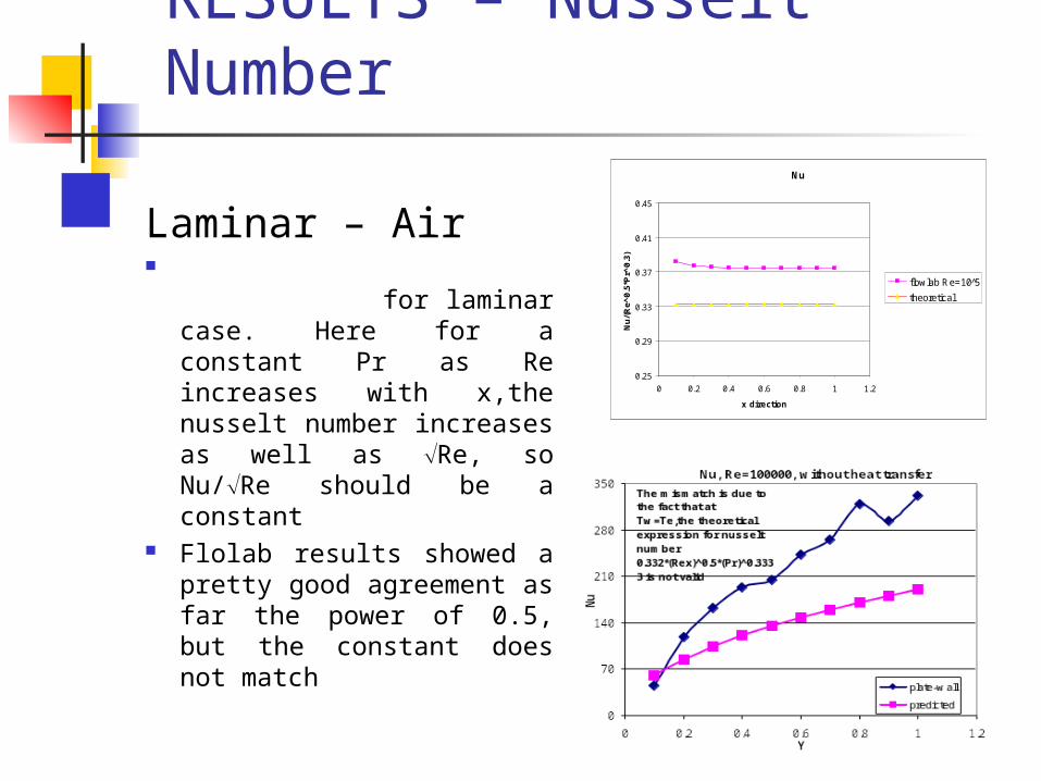
Laminar – Air
for laminar case. Here for a constant Pr as Re increases with x,the nusselt number increases as well as Re, so Nu/Re should be a constant
Flolab results showed a pretty good agreement as far the power of 0.5, but the constant does not match
Nu
0.25
0.29
0.33
0.37
0.41
0.45
0 0.2 0.4 0.6 0.8 1 1.2
x direction
Nu
/(R
e^0.
5*P
r^0.
3)
flowlab Re=10 5̂
theoretical
RESULTS – Reynolds Similarity
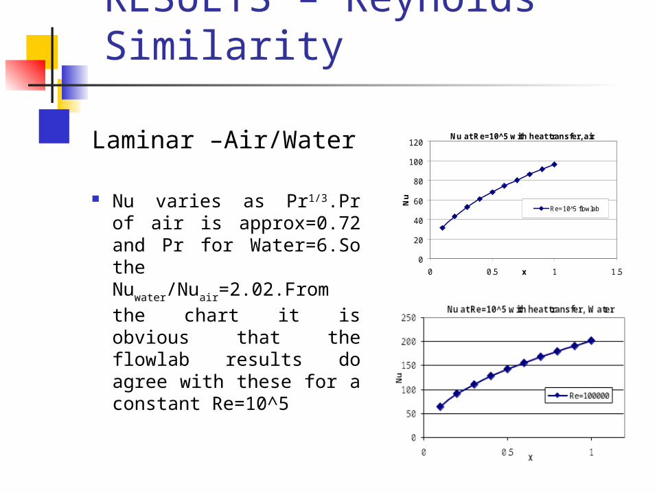
Laminar –Air/Water
Nu varies as Pr1/3.Pr of air is approx=0.72 and Pr for Water=6.So the Nuwater/Nuair=2.02.From the chart it is obvious that the flowlab results do agree with these for a constant Re=10^5
Nu at Re=10^5 with heat transfer, air
0
20
40
60
80
100
120
0 0.5 1 1.5x
Nu
Re=10^5 flowlab
RESULTS – Nusselt Number
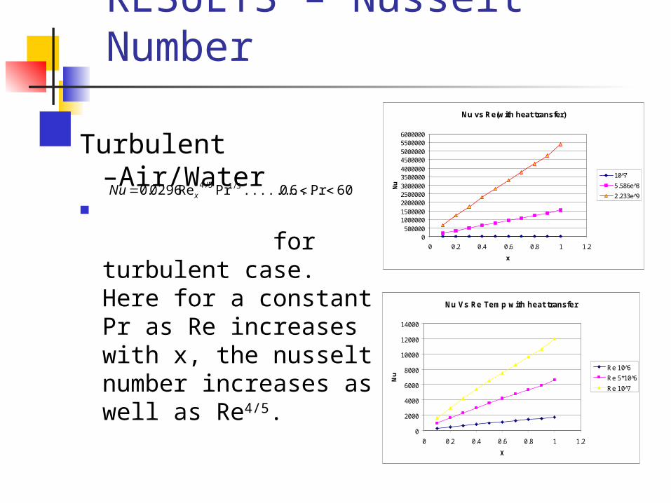
Turbulent –Air/Water
for turbulent case. Here for a constant Pr as Re increases with x, the nusselt number increases as well as Re4/5.
Nu vs Re(with heat transfer)
0500000
10000001500000200000025000003000000350000040000004500000500000055000006000000
0 0.2 0.4 0.6 0.8 1 1.2
x
Nu
10 7̂
5.586e 8̂
2.233e 9̂
Nu Vs Re Temp with heat transfer
0
2000
4000
6000
8000
10000
12000
14000
0 0.2 0.4 0.6 0.8 1 1.2
X
Nu
Re 10 6̂
Re 5*10 6̂
Re 10 7̂
60Pr6.0...........PrRe0296.0 3/15/4 xNu
RESULTS – Nusselt Number
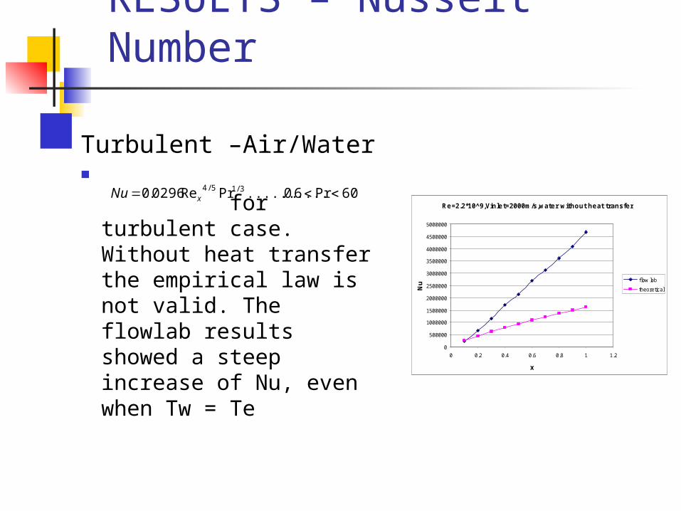
Turbulent –Air/Water
for turbulent case. Without heat transfer the empirical law is not valid. The flowlab results showed a steep increase of Nu, even when Tw = Te
60Pr6.0...........PrRe0296.0 3/15/4 xNuRe=2.2*10^9,Vinle t=2000m/s,water without heat transfer
0
500000
1000000
1500000
2000000
2500000
3000000
3500000
4000000
4500000
5000000
0 0.2 0.4 0.6 0.8 1 1.2
x
Nu
f low lab
theoretical
RESULTS – Nusselt Number
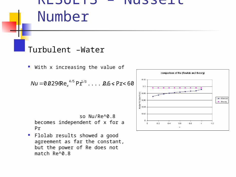
Turbulent –Water
With x increasing the value of
so Nu/Re^0.8 becomes independent of x for a Pr
Flolab results showed a good agreement as far the constant, but the power of Re does not match Re^0.8
60Pr6.0...........PrRe0296.0 3/15/4 xNu
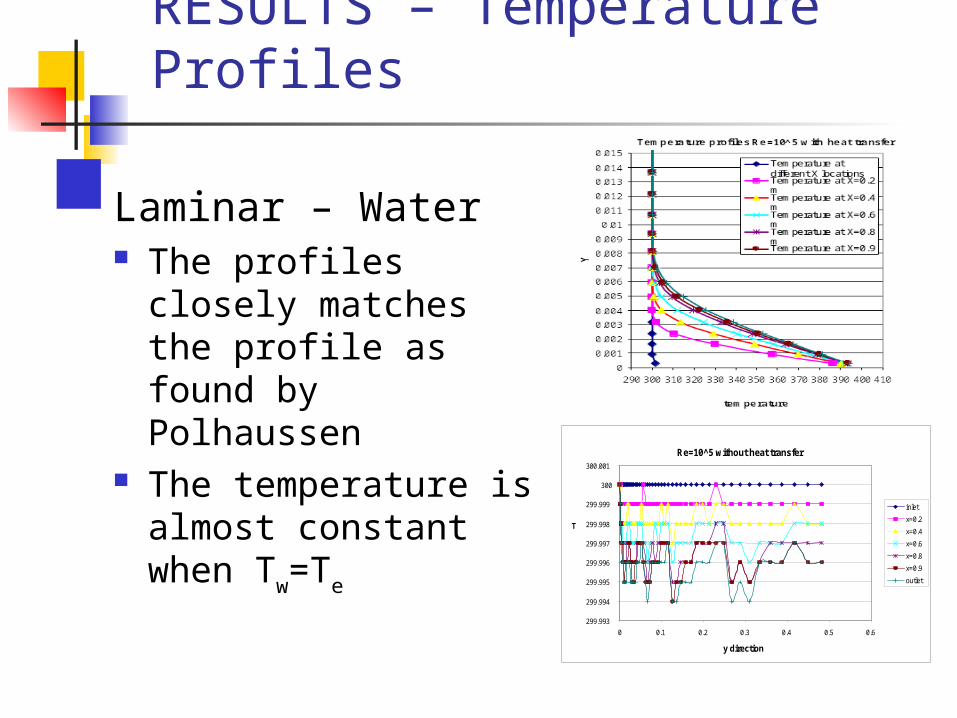
RESULTS – Temperature Profiles
Laminar – Water The profiles closely
matches the profile as found by Polhaussen
The temperature is almost constant when Tw=Te
Re=10^5 without heat transfer
299.993
299.994
299.995
299.996
299.997
299.998
299.999
300
300.001
0 0.1 0.2 0.3 0.4 0.5 0.6
y direction
T
inlet x=0.2 x=0.4 x=0.6 x=0.8 x=0.9 outlet
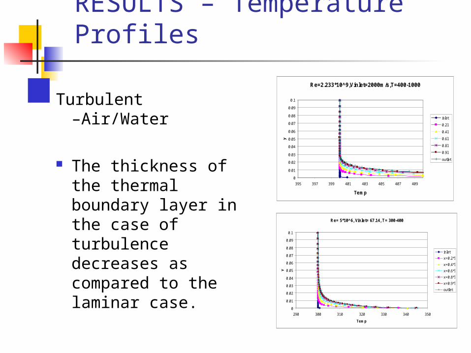
RESULTS – Temperature Profiles
Turbulent –Air/Water
The thickness of the thermal boundary layer in the case of turbulence decreases as compared to the laminar case.
Re=2.233*10^9,Vinlet=2000m/s,T=400-1000
0
0.01
0.02
0.03
0.04
0.05
0.06
0.07
0.08
0.09
0.1
395 397 399 401 403 405 407 409
Temp
y
inlet
0.2l
0.4l
0.6l
0.8l
0.9l
outlet
Re= 5*10^6, Vinlet= 67.14, T= 300-400
0
0.01
0.02
0.03
0.04
0.05
0.06
0.07
0.08
0.09
0.1
290 300 310 320 330 340 350
Temp
Y
inlet
x=0.2*l
x=0.4*l
x=0.6*l
x=0.8*l
x=0.9*l
outlet
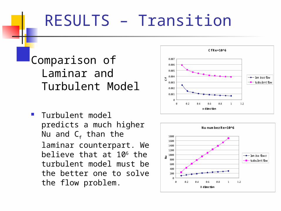
RESULTS – Transition
Comparison of Laminar and Turbulent Model
Turbulent model predicts a much higher Nu and Cf than the laminar counterpart. We believe that at 106 the turbulent model must be the better one to solve the flow problem.
Cf Re=10^6
0
0.001
0.002
0.003
0.004
0.005
0.006
0.007
0 0.2 0.4 0.6 0.8 1 1.2
x direction
Cf laminar flow
turbulent flow
Nu number Re=10^6
0
200
400
600
800
1000
1200
1400
1600
1800
0 0.2 0.4 0.6 0.8 1 1.2
X direction
Nu lamina flowr
turbulent flow
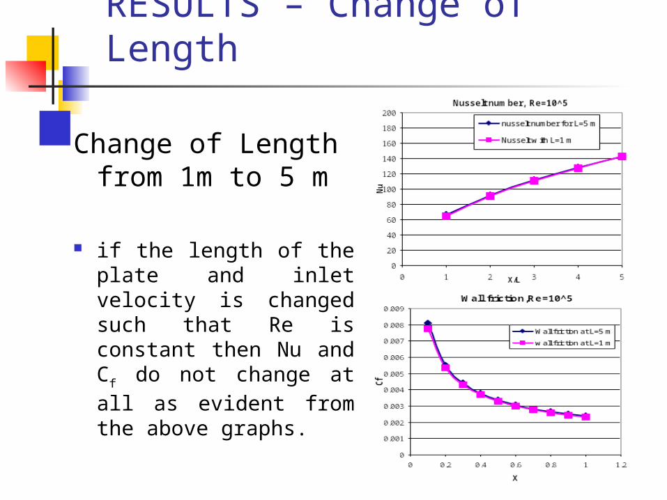
RESULTS – Change of Length
Change of Length from 1m to 5 m
if the length of the plate and inlet velocity is changed such that Re is constant then Nu and Cf do not change at all as evident from the above graphs.
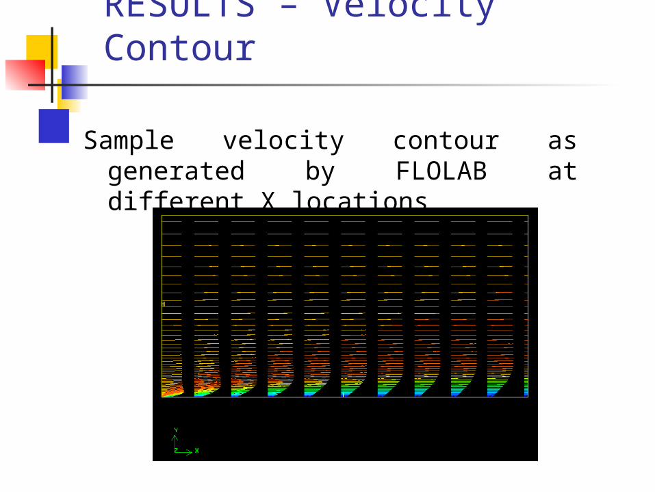
RESULTS – Velocity Contour
Sample velocity contour as generated by FLOLAB at different X locations
Conclusions
Flowlab shows fairly good agreement in all respects as compared to the theoretical values obtained by the boundary layer theory
However it is not possible to get *, , directly from the flowlab results.
The overshoot in the velocity profiles above the inlet velocity also couldn’t be explained .