Embed Size (px)
Citation preview

Flexible Digital Display Technologies Using Open Source
Hardware and Software for Automotive Applications
A DISSERTATION
SUBMITTED TO THE DEPARTMENT OF ENGINEERING TECHNOLOGY
OF WATERFORD INSTITUTE OF TECHNOLOGY
IN COMPLETE FULFILLMENT OF THE REQUIREMENTS
FOR THE DEGREE OF
MASTER OF ENGINEERING
By:
Patrick D. Mc Donnell
Supervised By:
Mr. Henry Acheson
June 2009

Dedicated To:
My Father: John Mc Donnell
And
My Mother: Lish Mc Donnell

i
Declaration
I hereby certify that the material presented in this document is entirely my own work
and has not been submitted previously as an exercise or degree at this or any other
establishment of higher education. I the author alone have undertaken the work except
where otherwise stated.
Signed: ________________________
Date: ________________

ii
Acknowledgements I hereby acknowledge the contributions to my work and offer my thanks to people who
have helped and supported me during my work over the past two years.
My Supervisor:
Mr. Henry Acheson: I would like to thank Henry for his constant encouragement,
invaluable guidance and excellent supervision during the last two years.
My Family:
I would like to thank my family for their support, encouragement and understanding
throughout all of my studies.
The AAEC (Advanced Automotive Electronic Control) Research Group:
I would like to take this opportunity to thank all members, both past and present, of the
research group whose assistance, knowledge and support has been first rate. I would
like to pay a particular thanks to John Manning, Gavin Walsh and Niall Murphy for
their additional support throughout the project.
My Friends:
A special word of thanks goes to my girlfriend, Aideen, and all my friends. Their humor
and encouragement will never be forgotten.
Additional Support:
I would like to thank Robin Getz and Jason Berry for their in-depth knowledge and
support during the project.
There are also many more people who have contributed in countless others way and
deserve my thanks also – Thank you!

iii
Abstract With the advances in electronics, digital dashboards are now becoming available for use
in the automotive industry. The main difference between an analog dashboard and a
digital dashboard configuration is that the later may easily be reconfigured.
To accommodate the influx of digital graphical displays in vehicles, manufacturers have
started to run micro Real Time Operating Systems (RTOS) inside their vehicles. Two
options are offered to manufacturers when choosing a RTOS for their project;
commercial OSs or open source OSs. Commercial OS contain many overheads which
include an upfront capital investment and licensing fee for each unit produced. While
open source OS are royalty free and offer no such financial overheads. Any application
software that is written by the manufacturer for a commercial OS, is seen as proprietary
software, and hence is not accessible by other manufacturers. Whilst any software
written and licensed for use with an open source OS would be accessible, therefore
leading to reduction in manufacturing costs and time.
The main objective of this research was to develop a flexible digital display using open
source hardware and software for use in automotive applications. The development of a
digital dashboard using these technologies can allow for individual customisation and in
addition facilitate a significant reduction in the design cycle time. The designed display
controller incorporated an Analog Devices Blackfin development board onto which an
open source OS was ported. Automotive information was read from a CAN network
and was used to manipulate the data displayed on the digital dashboard.

iv
Table of Contents
Declaration.................................................................................................................... i
Acknowledgements...................................................................................................... ii
Abstract....................................................................................................................... iii
Table of Contents ....................................................................................................... iv
List of Figures............................................................................................................. ix
List of Tables ............................................................................................................ xiii
List of Abbreviations ............................................................................................... xiv
1 Introduction..........................................................................................................1
1.1 Introduction....................................................................................................2
1.2 Thesis Contributions ......................................................................................4
2 Technical Literature Review...............................................................................5
2.1 Introduction....................................................................................................6
2.2 Selection of a Processor .................................................................................6
2.2.1 Automotive Conditions Specifications ..................................................7
2.2.2 CAN Support..........................................................................................8
2.2.3 Graphical Display Support.....................................................................9
2.2.4 Clock Capabilities ................................................................................10
2.2.5 Memory ................................................................................................11
2.2.6 Synopsis of Reviewed Processors........................................................12
2.3 Development Host........................................................................................13
2.3.1 coLinux ................................................................................................13
2.3.1.1 Pseudo Physical RAM .....................................................................14
2.3.1.2 Context Switching............................................................................15
2.3.1.3 Interrupt Handling............................................................................16
2.3.1.4 Advantages of using coLinux ..........................................................17
2.3.1.5 Disadvantages of using coLinux ......................................................17
2.4 uClinux.........................................................................................................18
2.4.1 Differences between uClinux and Linux..............................................18
2.4.1.1 No Memory Management Unit ........................................................18
2.4.1.2 Kernel Differences ...........................................................................19
v
2.4.1.3 Memory Allocation (Kernel)............................................................19
2.4.1.4 Memory Allocation (Application)....................................................20
2.4.1.5 Applications and Processes ..............................................................21
2.4.2 Booting uClinux...................................................................................21
2.4.2.1 U-Boot..............................................................................................22
2.5 Graphics Libraries........................................................................................22
2.5.1 DirectFB...............................................................................................23
2.5.1.1 Access to Graphics Hardware by DirectFB .....................................23
2.5.1.2 DirectFB Features ............................................................................24
2.5.2 SDL ......................................................................................................25
2.5.2.1 SDL Libraries...................................................................................26
2.5.2.2 SDL Features....................................................................................27
2.5.3 Selecting the Graphical Library ...........................................................28
2.6 Inter Process Communications.....................................................................29
2.6.1 Semaphores ..........................................................................................29
2.6.2 Shared Memory....................................................................................30
2.6.3 Message Queues...................................................................................31
2.6.4 Named Pipes ........................................................................................32
2.6.5 Selecting an IPC...................................................................................33
2.7 Controller Area Network..............................................................................34
2.7.1 CAN Bit Encoding ...............................................................................35
2.7.2 CAN Bit Rates and Timings ................................................................37
2.7.3 Propagation Delay................................................................................39
2.7.4 Synchronisation....................................................................................40
2.7.4.1 Hard Synchronisation.......................................................................40
2.7.4.2 Resynchronisation............................................................................41
2.7.5 CAN Message Framing........................................................................41
2.7.5.1 Data Frame.......................................................................................42
2.7.5.2 Remote Frame ..................................................................................43
2.7.5.3 Overload Frame................................................................................44
2.7.5.4 Error Frame ......................................................................................44
2.8 Summary ......................................................................................................44

vi
3 System Configuration and Design ....................................................................45
3.1 Introduction..................................................................................................46
3.2 System Configuration Overview..................................................................47
3.3 coLinux ........................................................................................................47
3.3.1 Installing coLinux ................................................................................48
3.3.2 Configuring coLinux............................................................................48
3.3.2.1 Configuring the Network .................................................................48
3.3.2.2 Configuring the FTP server..............................................................51
3.3.2.3 Installing the Blackfin Toolchains ...................................................52
3.4 U-Boot..........................................................................................................53
3.4.1 Compiling U-Boot................................................................................53
3.4.1.1 Compiling U-Boot for Loading over the UART..............................54
3.4.2 Loading U-Boot onto the BF548 .........................................................55
3.4.3 Saving U-Boot to Flash........................................................................57
3.4.4 Configuring the Network Settings in U-Boot ......................................57
3.4.5 Testing U-Boot.....................................................................................59
3.5 The uClinux Kernel......................................................................................60
3.5.1 Configuring and Compiling the uClinux Kernel..................................60
3.5.2 Testing the new uClinux Kernel ..........................................................63
3.6 CAN Functionality .......................................................................................64
3.6.1 Initial CAN Setup.................................................................................64
3.6.1.1 Activating the CAN Driver ..............................................................65
3.6.2 Initial Testing .......................................................................................66
3.6.2.1 Baud Rate Error ...............................................................................67
3.6.2.2 CAN Header Files ............................................................................68
3.6.2.3 Editing the System Clock.................................................................69
3.6.3 Testing CAN on the BF548 .................................................................73
3.6.3.1 Testing the can_send program .........................................................74
3.6.3.2 Testing the receive program.............................................................75
3.7 Simple Directmedia Layer ...........................................................................77
3.7.1 Graphical Representations ...................................................................77
3.7.2 Digital Representation of a Standard Dash Configuration...................78
3.7.2.1 Graphics Creation ............................................................................78
3.7.2.2 Initial SDL Code (Analog Dials) .....................................................79

vii
3.7.2.3 Using a Random Number Generator to Vary the Speed ..................81
3.7.2.4 Integrated Dial Code ........................................................................82
3.7.3 Digital Bar Chart Representation.........................................................85
3.7.3.1 Graphics Creation ............................................................................85
3.7.3.2 Initial SDL Code (Bar Chart)...........................................................87
3.7.3.3 Basic Bar Chart Code.......................................................................88
3.7.3.4 Changing the Bar Colour with Speed...............................................90
3.7.3.5 Decrementing the Speed ..................................................................91
3.7.3.6 Using a Random Number Generator to Vary the Speed ..................92
3.7.3.7 Displaying Error Messages with the Bar Chart................................96
3.8 Inter Process Communications.....................................................................97
3.8.1 Writing to a Pipe ..................................................................................98
3.8.1.1 Naming and Creating a Pipe ............................................................98
3.8.1.2 Writing to the Created Pipe..............................................................99
3.8.2 Reading from a Pipe...........................................................................100
3.8.3 Disadvantages of Named Pipes..........................................................102
3.8.3.1 Editing the Write Program to allow the Transmission of Integers.102
3.8.4 Editing the Read Program to allow the Manipulation of Integers .....103
3.8.5 Testing the Transmission and Reception of Integers .........................103
3.8.5.1 Editing the Write Program .............................................................103
3.8.5.2 Editing the Read Program ..............................................................104
3.8.5.3 Running the Test Programmes .......................................................104
3.9 Summary ....................................................................................................105
4 System Implementation and Testing ..............................................................107
4.1 Introduction................................................................................................108
4.2 CAN Implementation.................................................................................108
4.2.1 CAN Message Breakdown.................................................................108
4.2.2 CAN Sample Code.............................................................................109
4.2.3 Editing the Sample Code....................................................................110
4.2.3.1 Creating the Named Pipes..............................................................112
4.2.3.2 Populating the Variables used when Writing to the Named Pipes.112
4.2.3.3 Populating the Variable used for the CAN ID ...............................113
4.2.3.4 Populating the Speed Variable .......................................................113

viii
4.2.3.5 Populating the rpm Variable ..........................................................114
4.2.3.6 Writing the Populated Variables to their Named Pipes .................115
4.2.4 Testing the CAN with Named Pipes Code.........................................115
4.3 SDL Implementation..................................................................................117
4.3.1 Merging the Digital Dash and Bar Chart Code..................................117
4.3.2 Opening and Reading Named Pipes in SDL......................................118
4.3.3 Manipulating the Received Data........................................................118
4.3.3.1 Manipulating the CAN ID..............................................................119
4.3.3.2 Manipulating the Speed Data .........................................................120
4.3.3.3 Manipulating the rpm data .............................................................124
4.4 Testing the Final System............................................................................125
4.4.1 Initial Testing .....................................................................................126
4.4.2 Testing the Final System....................................................................129
4.5 Stress Testing the End System ...................................................................133
4.5.1 Testing System for Initial Goals ........................................................134
4.5.2 Testing the System for Limitations ....................................................136
4.6 Summary ....................................................................................................138
5 Conclusion.........................................................................................................139
5.1 Introduction................................................................................................140
5.2 Conclusions................................................................................................140
5.3 Recommendations for further Research and Development .......................144
References .................................................................................................................145
Appendix A – Write to Pipes Program ..................................................................152
Appendix B – Read from Pipes Program...............................................................154
Appendix C – CAN Program ..................................................................................155
Appendix D – Video Program.................................................................................164

ix
List of Figures
Fig. 1.1 Currently used OSs ...........................................................................................3
Fig. 1.2 Planned Future use of OS ................................................................................3
Fig. 2.1 Integrated Vs Peripheral CAN..........................................................................8
Fig. 2.2 coLinux running natively on Windows OS ....................................................14
Fig. 2.3 Address Space Transition used in Context Switching....................................16
Fig. 2.4 Memory Allocation using Power-Of-Two Method ........................................20
Fig. 2.5 Memory Allocation using Kmalloc2 ..............................................................20
Fig. 2.6 DirectFB System Diagram..............................................................................23
Fig. 2.7 DirectFB Access to the Framebuffer Device and the Graphics Hardware .....24
Fig. 2.8 Abstraction Layer of Windows and Linux SDL Platforms ............................26
Fig. 2.9 SDL Application .............................................................................................28
Fig. 2.10 IPC at process level ......................................................................................29
Fig. 2.11 Semaphore Metaphor....................................................................................30
Fig. 2.12 Shared Memory ............................................................................................31
Fig. 2.13 Message Queue.............................................................................................32
Fig. 2.14 Blocking Vs. Non-Blocking Named Pipes ...................................................33
Fig. 2.15 Point-to-Point Wiring System.......................................................................34
Fig. 2.16 CAN Network...............................................................................................35
Fig. 2.17 Differential Bus Signalling ...........................................................................36
Fig. 2.18 ISO11898 Nominal Bus Levels ....................................................................37
Fig. 2.19 CAN Message Layout...................................................................................37
Fig. 2.20 CAN Message in TQ ....................................................................................39
Fig. 2.21 Propagation Delay between Nodes ...............................................................40
Fig. 2.22 SJW used in Resynchronisation....................................................................41
Fig. 2.23 Standard CAN Data Frame...........................................................................42
Fig. 3.1 System Configuration Overview ....................................................................47
Fig. 3.2 Sharing Ethernet Connection..........................................................................49
Fig. 3.3 Configuring the coLinux TAP Interface.........................................................49
Fig. 3.4 Edited coLinux Interfaces File........................................................................50
Fig. 3.5 Edited coLinux Resolv.conf File ....................................................................50
Fig. 3.6 Pinging coLinux from Windows ....................................................................51

x
Fig. 3.7 Pinging Windows from coLinux ....................................................................51
Fig. 3.8 Configured FTP Server...................................................................................52
Fig. 3.9 Setting Boot Mode to UART..........................................................................54
Fig. 3.10 Configuring and Compiling U-Boot .............................................................54
Fig. 3.11 Configuring LdrViewer ................................................................................55
Fig. 3.12 Testing Communications between LdrViewer and BF548...........................56
Fig. 3.13 U-Boot Transferred Successfully .................................................................56
Fig. 3.14 Network Configuration of Development Host..............................................58
Fig. 3.15 Configuring the Network in U-Boot.............................................................58
Fig. 3.16 Downloading the uImage..............................................................................59
Fig. 3.17 Booted Kernel ...............................................................................................60
Fig. 3.18 Main Menu for Configuring the uClinux Kernel..........................................61
Fig. 3.19 Selecting Vendor and Product ......................................................................61
Fig. 3.20 Including SDL Library Files.........................................................................62
Fig. 3.21 Including SDL and CAN Examples..............................................................62
Fig. 3.22 Compiling New Kernel.................................................................................63
Fig. 3.23 Running Hello World Test Program.............................................................64
Fig. 3.24 Activating the CAN driver............................................................................66
Fig. 3.25 Error Frames at 125kbaud ............................................................................67
Fig. 3.26 CAN signal from BF548...............................................................................67
Fig. 3.27 CAN RX at 133kbps .....................................................................................68
Fig. 3.28 CAN RX from BF548 at 125kbps ................................................................73
Fig. 3.29 can_send Command......................................................................................74
Fig. 3.30 Sending CAN messages using can_send ......................................................74
Fig. 3.31 Messages received on CANalyzer ................................................................75
Fig. 3.32 Example of Received Message .....................................................................75
Fig. 3.33 Messages used to Test the Receive Program................................................76
Fig. 3.34 Messages Received using receive program ..................................................76
Fig. 3.35 Speed dial at 0 mph.......................................................................................78
Fig. 3.36 rpm dial at 0 rpm...........................................................................................79
Fig. 3.37 End users display ..........................................................................................79
Fig. 3.38 Flow Chart of Basic SDL Dial program .......................................................80
Fig. 3.39 Flow Chart for Integrated Dial Code ............................................................83
Fig. 3.40 Bar Chart.......................................................................................................86
xi
Fig. 3.41 Speed below 70mph......................................................................................86
Fig. 3.42 Speed greater than 70mph and below 100mph.............................................86
Fig. 3.43 Speed greater than 100mph...........................................................................86
Fig. 3.44 Bar Chart with Error Message ......................................................................87
Fig. 3.45 Output from Initial Code ..............................................................................88
Fig. 3.46 Basic Bar Chart Flow Chart..........................................................................89
Fig. 3.47 Flow Chart for Bar Chart Representation of Speed......................................93
Fig. 3.48 Users Prompt for Selecting Errors ................................................................97
Fig. 3.49 Background set as Error 2.............................................................................97
Fig. 3.50 Running Write to Pipes code on BF548 .....................................................100
Fig. 3.51 Displaying the Contents of the Named Pipe...............................................100
Fig. 3.52 Running Write program in conjunction with Read program ......................101
Fig. 3.53 Read from Pipes..........................................................................................102
Fig. 3.54 User Prompt to enter Integer.......................................................................105
Fig. 3.55 Output from Read Program ........................................................................105
Fig. 4.1 Breakdown of CAN message........................................................................109
Fig. 4.2 Receive Flow Chart ......................................................................................110
Fig. 4.3 Receive with Named Pipes Flow Chart ........................................................111
Fig. 4.4 Test Messages sent using CANalyzer...........................................................115
Fig. 4.5 Messages received and Wrote into Named Pipes .........................................116
Fig. 4.6 Read Pipes Program Displays Sent Data ......................................................116
Fig. 4.7 CAN ID used to select Display Configuration .............................................117
Fig. 4.8 Communications between both Processes ....................................................119
Fig. 4.9 Final System .................................................................................................126
Fig. 4.10 Error displayed during Initial Testing.........................................................126
Fig. 4.11 Initialised Screen ........................................................................................127
Fig. 4.12 Applying the Dials to the Screen ................................................................127
Fig. 4.13 Applying the Bar Chart to the Screen.........................................................127
Fig. 4.14 Changing to the Dials from the Bar Chart ..................................................128
Fig. 4.15 Applying the Bar Chart to the Screen.........................................................129
Fig. 4.16 Applying the mask......................................................................................129
Fig. 4.17 Applying the Dials to the Screen with the Mask ........................................129
Fig. 4.18 Messages sent using CANalyzer ................................................................130
Fig. 4.19 Messages Received by the CAN program ..................................................130

xii
Fig. 4.20 SDL program Reading Data from Pipes .....................................................130
Fig. 4.21 Output on the LCD Screen for Message 1..................................................131
Fig. 4.22 Output on the LCD Screen for Message 2..................................................131
Fig. 4.23 Output on the LCD Screen for Message 3..................................................132
Fig. 4.24 Flow Chart of End System..........................................................................133
Fig. 4.25 Setting the Period of each CAN Message to 100ms in CANalyzer............134
Fig. 4.26 Messages when Stress Testing the End System .........................................135
Fig. 4.27 Setting the Period of each CAN Message to 50ms in CANalyzer..............136
Fig. 4.28 Received Error using a Message Period of 50ms .......................................136
Fig. 5.1 System Configuration Overview ..................................................................142
Fig. 5.2 Final System .................................................................................................143

xiii
List of Tables Table 2.1 Ambient Operating Temperatures of Selected Processors.............................7
Table 2.2 CAN Capabilities of Selected Development Boards .....................................9
Table 2.3 Graphical Display Support of Selected Development Boards .....................10
Table 2.4 CPU Frequency of Selected Development Boards ......................................11
Table 2.5 Available Memory of Selected Development Boards..................................11
Table 2.6 Synopsis of Reviewed Processors................................................................12
Table 2.7 Segments of a CAN Message.......................................................................38
Table 3.1 coLinux Network Configurations ................................................................50
Table 3.2 Created Files from U-Boot Compilation......................................................55
Table 3.3 Logical OR Truth Table...............................................................................84
Table 3.4 Change Over Values of Coloured Bars........................................................90
Table 3.5 Logical AND Truth Table............................................................................95
Table 3.6 Bar Chart Error Screens ...............................................................................96
Table 4.1 2D Array used in Receive Program ...........................................................113

xiv
List of Abbreviations ACK Acknowledge
ANSI American National Standards Institute
ARGB Alpha Red Green Blue
bkg Background
bpp Bits Per Pixel
BRP Baud Rate Prescaler
CAN Controller Area Network
CANH CAN High
CANL CAN Low
CPU Central Processing Unit
DLC Data Length Code
DPLL Digital Phase Lock Loop
FIFO First In First Out
FTP File Transfer Protocol
GIF Graphics Interchange Format
HDD Hard Disk Drive
Hz Hertz
IC Integrated Circuit
IDT Interrupt Descriptor Table
IDTR Interrupt Descriptor Table Register
IP Internet Protocol
IPC Inter Process Communication
ISR Interrupt Service Routines
JPEG Joint Photographic Experts Group
LCD Liquid Crystal Display
LSB Least Significant Bit
MB Mega Bytes
MBR Master Boot Record
MMU Memory Management Unit
mph Miles Per Hour
MSB Most Significant Bit
NBR Nominal Bit Rate

xv
NBT Nominal Bit Time
NRZ Non Return to Zero
NTQ Number of Time Quanta
OS Operating System
PC Personal Computer
PNG Portable Network Graphics
PNM Portable aNy Map
PPRAM Pseudo Physical RAM
PS1 Phase Segment 1
PS2 Phase Segment 2
RAM Random Access Memory
ROM Read Only Memory
RPM RPM Package Manager
rpm Revolutions Per Minute
RTF Rich Text Format
RTOS Real Time Operating System
RTR Remote Transmission Request
SCLK System Clock
SDL Simple Directmedia Layer
SJW Synchronised Jump Width
SOF Start-of-Frame
SPI Serial Peripheral Interface
TCP Transmission Control Protocol
TFT Thin Film Transistor
TIFF Tagged Image File Format
TQ Time Quanta
TTF True Type Font
UART Universal Asynchronous Receiver/Transmitter
UDP User Datagram Protocol
VESA Video Electronics Standards Association
VM Virtual Memory
XPM X PixMap

1
1 Introduction

2
1.1 Introduction In the automotive industry an analog/mechanical dashboard display is still the standard.
This type of dashboard contains basic dials which usually include a speedometer,
tachometer, temperature gauge, fuel gauge and warning lamps which may include low
oil level, low fuel level, Engine Management, ABS etc. One of the limitations with this
type of dash display is that the positioning of all instrumentation is fixed and cannot be
reconfigured [1].
With the advances in electronics, digital dashboards are now becoming available for use
in the automotive industry. The main difference between analog and digital dashboards
is that the digital dashboard may easily be reconfigured. With a digital dashboard,
information can be displayed either numerically or via a digital representation of an
analog/mechanical dial. Hence, any dial can be removed if it is required to display a
warning signal to the driver [2]. An example of this is the Night Vision Assist system
used in the Mercedes S-Class. This system uses an infrared beam which goes beyond
the reach of the head lights along with a special camera mounted in the rear view mirror
which reads the infrared signals. The resulting image is displayed on the dashboard
instead of the normal speedometer, which is reconfigured to be a bar graph at the
bottom of the digital dashboard. This system is said to increase visibility by 125% while
driving at night [3].
The Night View Assist system developed by Mercedes is just one example of the
flexibility a digital dashboard has to offer. It could be used to display any information
on the screen in real time. In a high-end sports car this type of dashboard could be used
to display engine analysis and performance while in a family car it could display more
safety-orientated information.
To accommodate the influx of digital graphical displays in vehicles, manufacturers
began to utilise micro Real Time Operating Systems (RTOS) on the controlling
microprocessor system. The microprocessors derive the vehicles data by linking to the
CAN network.

3
Currently there are two options for manufacturers when choosing an RTOS for their
project; a commercial OS or an open source OS. Commercial OSs contain many
overheads which include an upfront capital investment and licensing fee for each unit
produced [4]. While open source OSs are royalty free and offer reduced financial
overheads.
Fig. 1.1 Currently used OSs
In a recent survey undertaken by the website embedded.com, major global
manufacturers were questioned on their use of RTOS in their embedded environments.
The current trend is shown in Fig. 1.1. When questioned on future projects their
responses were much different as can be seen in Fig. 1.2.
Fig. 1.2 Planned Future use of OS
Using the data in Fig. 1.1 and Fig. 1.2, it can be seen that the projected use of open
source OSs will rise from 20% to 41%, with the potential to rise as high as 74%. The
main reason cited for the move to open source is costs (savings) associated with it [5].
This research investigates the development of a flexible digital display using open
source hardware and software for use in automotive applications. The development of a
digital-dashboard using these technologies can allow for individual customisation and in
addition facilitate a significant reduction in the design cycle time and costs.

4
1.2 Thesis Contributions The material and information presented in this thesis has been compiled on the basis of:
(i) A comprehensive technical literature review of the current innovations in
dashboard technology.
(ii) Design, configuration and implementation of a proposed digital display
system using open source hardware and software.
(iii) Testing and conclusions.
The work presented in this thesis is laid out as follows:
Chapter 2 gives an overview of the most relevant information from all technical
literature reviewed during the research stage of this study. This chapter also outlines the
possible choices available during the design of the proposed system.
Chapter 3 provides an overview of the choices made and methods used to configure and
design the proposed system. It also gives a complete explanation of the operation of the
system with emphasis on the OS and application software.
Chapter 4 discusses how the final system was implemented and fully tested. This
includes the development of a CAN process, video process and Inter Process
Communications. The testing of the final system is also described in this chapter.
Chapter 5 outlines the conclusions made based on the research and testing. A discussion
on further possibilities for research based on findings from this study is also provided.

5
2 Technical Literature Review

6
2.1 Introduction The purpose of this chapter is to give an overview of the most relevant information from
all technical literature reviewed during the research stage of this study. This chapter will
also outline the possible choices available during the design of the proposed system.
The information based on the literature review presented in this chapter is laid out as
follows:
• Section 2.2 outlines the choices available when selecting a processor for this
project. This section covers the pros and cons of the processors under selected
headings. It also includes the selection process and the reasons for use of a
particular processor.
• Section 2.3 provides the background information on the development host
environment chosen for use in this project.
• Section 2.4 gives an overview of the operating system (OS) chosen for the
process used in this project. It also details the bootloader that was used in
conjunction with the OS.
• Section 2.6 discusses the possible options for Inter Process Communications and
outlines each option and offers insight on the selection process.
• Section 2.7 gives an overview of the Controller Area Network protocol required
for communication between the selected processor and external electronic
control modules.
• Section 2.8 concludes the chapter with a brief summary.
2.2 Selection of a Processor When selecting a processor for an automotive display application, key factors have to be
taken into consideration. In an automotive environment the selected processor will have
to endure very harsh conditions. The processor is required to perform at an optimal level
to deal with the high computational needs of a graphical display along with the data
transmission from the CAN network. It must also accommodate an appropriate
operating system. The key considerations taken into account when selecting the
processor are listed below:

7
• Automotive Conditions Compatibility
• Controller Area Network (CAN) support
• Graphical Display support
• Clock capabilities
• Memory
As the project was designed to use open source hardware and software, all of the
scrutinised processors fully supported the use of an open source operating system. The
development boards below contain suitable processors for the completion of this project
and were evaluated using the key considerations above to determine the most suitable.
• Cogent CSB337 [6], [16], [17]
• Analog Devices ADSP-BF548 EZ Kit [7], [8]
• Atmel AT91SAM9263 [9], [10], [11]
• Cirrus EDB9315 [12], [13]
2.2.1 Automotive Conditions Specifications Many conditions inside the automotive environment act as a hindrance to electronic
components, one of which is the working temperature range [14]. Each board’s
temperature range was evaluated to ensure their durability in such an environment. The
temperature range for Integrated Circuits (IC’s) in the automotive setting is -40°C to
125°C [14]. Each board’s specified temperature range was compared to the typical
temperature found in an automotive environment to evaluate their use, as shown in
Table 2.1.
Processor Temperature Range (°C) Cogent CSB337 0 to 70
Analog Devices ADSP-BF548 - 40 to + 85 Atmel AT91SAM9263 - 40 to + 85
Cirrus EDB9315 - 40 to + 85
Table 2.1 Ambient Operating Temperatures of Selected Processors

8
All of the boards’ ambient operating temperatures are in the typical temperature range
for an automotive setting, except for the Cogent CSB337. The Cogent CSB337 ambient
operating temperature range is far less than the other three processors.
2.2.2 CAN Support The CAN protocol is an automotive standard for vehicle communications, therefore, it
was desirable to have an integrated CAN controller on the chosen development board.
However if this was not possible, an SPI bus on the development board could be
implemented for CAN communications [15]. This would lead to extra costs in designing
and implementing a peripheral CAN controller, as well as having to implement a driver
for the SPI CAN.
Fig. 2.1 Integrated Vs Peripheral CAN
As illustrated in Fig. 2.1, the use of peripheral CAN leads to an increase of components
required. Also with a development board which supports an open source OS and has
integrated CAN, it will be likely that the drivers for the integrated CAN will be
contained in the kernel. When using the SPI port there will be no need for SPI-CAN
drivers. The table below shows the CAN capabilities of the development boards under
evaluation.

9
Processor Integrated CAN Total Number of Rx/Tx Buffers
Cogent CSB337 Yes 2Rx 2TX
Analog Devices ADSP-BF548 Yes
8 Rx 8 Tx
16 Configurable
Atmel AT91SAM9263 Yes 16 Configurable
Cirrus EDB9315 No N/A
Table 2.2 CAN Capabilities of Selected Development Boards
With reference to Table 2.2, it can be seen that three of the four boards contain
integrated CAN ports. The Cirrus EDB9315 does not contain an integrated CAN port
but it does however have an SPI port, therefore CAN communications could still be a
possibility. Comparing the three evaluation boards that do contain integrated CAN, it
can be seen that the ADSP-BF548 (BF548) contains more CAN buffers than its rivals
and hence makes its CAN handling abilities more powerful than the others.
2.2.3 Graphical Display Support As this project was designed to display automotive data, it was essential that the chosen
development board had the capabilities to support a graphical display. Also as it was
designed to replace the standard dash configuration in a vehicle, the graphical display
had to be quite powerful and needed to be able to accommodate in-depth images. An
LCD screen was essential and as with CAN, an integrated screen was ideal as the
appropriate drivers would probably be contained in the kernel.

10
Processor LCD Controller
Integrated LCD Screen Resolution (bpp)
Cogent CSB337 Yes No 8
Analog Devices ADSP-BF548 Yes Yes 24
Atmel AT91SAM9263 Yes Yes 16 (without limitation)
Cirrus EDB9315 Yes Yes 24
Table 2.3 Graphical Display Support of Selected Development Boards
As illustrated in Table 2.3, all of the boards under evaluation do have an integrated LCD
controller, however the Cogent CSB337 does not have an integrated LCD screen. If the
CSB337 was to be used, an external LCD screen would have to be included, therefore
increasing the cost of the project. Comparing the other three development boards, it can
be seen that the Atmel AT91SAM9263 supports 16bpp (bits per pixel) without
limitations, it can supports 24bpp but this is at the cost of losing the Ethernet port. This
leaves the BF548 and EDB9315 on par in their capabilities of display graphics.
2.2.4 Clock Capabilities As this project will have an OS running on the development board’s core along with
application programmes running on top of the OS, it is desirable to have a processor
with a relatively high clock frequency. As the OS used in the project is a Real Time OS
(RTOS) and all application programmes will be run in real time, it is beneficial to have
a high clock frequency. As in all cases, there are some tradeoffs in power consumption
when using high frequency clocks, but a high bandwidth real time system is more
important than power consumption for this application.

11
Processor Max. CPU Clock Frequency (MHz)
Cogent CSB337 180
Analog Devices ADSP-BF548 533
Atmel AT91SAM9263 200
Cirrus EDB9315 200
Table 2.4 CPU Frequency of Selected Development Boards
Table 2.4 shows that the BF548 has considerably the highest clocking frequency of all
the processors. The AT91SAM9263 and EDB9315 have the same processor clock
frequency, with the CSB337 clock frequency being slightly lower. As speed is essential
for the project, the BF548’s processor is the most desirable of the four boards.
2.2.5 Memory As an OS is required, it is vital that the development board has a sizeable amount of
memory. This memory is needed due to the fact that a boot loader, OS, application code
and a number of images will all be stored on the development board.
Processor SDRAM (MB)
Flash (MB)
Memory Card
Support Hard Drive
Cogent CSB337 32 8 No No
Analog Devices ADSP-BF548 64 32 Yes Yes (40GB)
Atmel AT91SAM9263 64 256 Yes No (does have HDD Port)
Cirrus EDB9315 64 32 No No
Table 2.5 Available Memory of Selected Development Boards

12
As shown in Table 2.5, the Atmel AT91SAM9263 has a very large amount of flash
memory when comparing it to any of the other development boards. It also supports a
memory card (i.e. it has an SD memory card reader) and has a port to add a hard drive,
however there is no HDD supplied. The BF548, while having less flash memory when
comparing it to the AT91SAM9263, does however have a 40GB HDD supplied with its
development board. The Cirrus EDB315 does have a substantial amount of integrated
memory but does not offer any expansion on this, while the CDB337 has very little
integrated memory. This leaves the BF548 and AT91SAM9263 equal, based on their
size of memory.
2.2.6 Synopsis of Reviewed Processors It was concluded from Table 2.6, that the Cogent CSB337 would not suffice for this
project, as it did not contain the desired functionality needed. The BF548,
AT91SAM9263 and EDB9315 are all sufficiently equipped for use in this project;
however the BF548 was the processor of choice.
Processor Auto. Spec.
CAN Handling Abilities
Graphical Display
Clock Capability Memory
Cogent CSB337 Poor Sufficient Poor Poor Poor
Analog Devices ADSP-BF548
Sufficient Excellent Excellent Excellent Excellent
Atmel AT91SAM
9263 Sufficient Sufficient Sufficient Poor/
Sufficient Excellent
Cirrus EDB9315 Sufficient Poor Excellent Poor/
Sufficient Sufficient
Table 2.6 Synopsis of Reviewed Processors

13
This was due to the EDB9315 needing peripheral CAN to be added to the board and
also its lower clock speed when comparing it to the BF548. Likewise, the
AT91SAM9263 had lower clocking capabilities and graphical display resolution when
compared to the BF548. As the BF548 had outstanding CAN handling abilities, along
with very high screen resolution, a 533MHz processor and large amount of memory,
including a 40GB hard drive, it was the obvious choice for use in this project. The next
section will discuss the development host, which will be used to develop and compile
the software to run on the BF548 processor.
2.3 Development Host As the BF548 was selected as the processor of choice, it was recommended by Blackfin
to use Cooperative Linux (coLinux) as the development host. Apart from coLinux,
many other Linux operating systems could have been used, including Red Hat, Ubuntu,
etc [18]. Along with the recommendation from the processor’s manufacturer, it offered
many other merits for its use as explained in the following sections.
2.3.1 coLinux Cooperative Linux (coLinux) is the first open source method used for optimally running
a Linux kernel natively alongside another OS, including Microsoft Windows, as shown
in Fig. 2.2. CoLinux is a port of the Linux kernel which can freely run without the use
of any virtualisation software, in a way which is much more optimal than using any
virtualisation software [19].

14
Fig. 2.2 coLinux running natively on Windows OS
Special driver software is used so that the coLinux kernel runs in a privileged mode on
the host OS. Due to its operation in privileged mode, and by constantly switching
between the host OS state and the coLinux kernel state, full control of the machine
Memory Management Unit (MMU) is granted to coLinux in its own allocated address
space. Therefore, coLinux acts in accordance to a native Linux kernel, while achieving
almost the same performance and functionality that would be expected from a
standalone Linux machine [18], [19].
2.3.1.1 Pseudo Physical RAM As coLinux runs alongside Microsoft Windows, it does not work on the principle of the
entire physical RAM being bestowed upon it during boot up, as is the case when
Microsoft Windows boots. Instead coLinux is allocated a fixed set of physical pages
and the translations needed to operate transparently in that set. This leads to coLinux
considering the allocated pages to be the entire physical memory and this is known as
Pseudo Physical RAM (PPRAM).
The PPRAM is allocated to coLinux using the standard function calls in each OS such
that it is not mapped in any address space on the host. These allocated pages will always
be resident and will only be freed once coLinux is closed. To map the allocated pages in
coLinux virtual address space, page tables are used, therefore its address space
resembles that of a regular kernel. The coLinux address space also has its own special

15
fixmaps, such that the page tables themselves are mapped in order to provide the ability
to translate from PPRAM addresses to physical addresses. Likewise, a special physical-
to-PPRAM map is allocated and mapped to decrease the time needed for handling
events which require physical addresses to be translated into PPRAM addresses. Due to
bi-directional memory address mapping, negligible overhead is achieved in page faults
and user space mapping operations [20], [18], [19].
2.3.1.2 Context Switching When coLinux is running on a host OS, it only uses one of the host processes to provide
a context for itself and its process. This one process, which is named as the coLinux-
daemon, is known as a Super Process as it frequently calls the kernel driver to perform a
context switch from the host OS to the coLinux kernel and back. This capability allows
complete control of the CPU and MMU of the machine without affecting the host OS.
For the Intel 386 architecture a complete context switch requires the top directory table
pointer register (CR3) to be changed. However, both the instruction pointer (EIP) and
CR3 cannot easily be changed in the one instruction. Therefore, CR3 has to be mapped
in both contexts for the change to be possible. Design limitations make it problematic to
map the code at the same virtual address in both contexts. However both contexts can
divide the kernel and the user space differently, such that one virtual address can
contain a user mapped page in one OS and a kernel mapped page in the other. When
context switching coLinux uses an intermediate address space, known as the “passage
page” as shown in Fig. 2.3.

16
Fig. 2.3 Address Space Transition used in Context Switching
The “passage page” is defined by specially created page tables in both coLinux and the
development host contexts. It maps the same code that is used for the switch at both of
the virtual addresses that are involved. When a switch occurs, first CR3 is changed to
point at the “passage page”. EIP is then relocated to the other mapping of the passage
code using a jump. Finally CR3 is changed to point to the top page directory of coLinux
[20], [19].
2.3.1.3 Interrupt Handling As a complete MMU context switch involves the Interrupt Descriptor Table Register
(IDTR), coLinux sets an interrupt vector table to handle any hardware interrupts that
occur while the system is in a running state. CoLinux will not act on these interrupts,
but instead it will only forward the interrupts invocations to the host OS, with the host
OS having to act on any interrupts for proper functionality. This enables the support of
the coLinux-daemon itself.
The interrupt vectors for the internal processor exceptions and system call vectors are
not edited such that coLinux handles its own page faults and other exceptions. However,
the other interrupt vectors point to a special proxy Interrupt Service Routines (ISRs). If
an ISR is invoked during coLinux time on the processor by an external hardware

17
interrupt, a context switch is made to the host OS. On the host side, the address of the
relevant ISR is determined by looking at its Interrupt Descriptor Table (IDT). With this
an interrupt call stack is forged and a jump occurs to the address. The interrupt flag is
disabled during the invocation of the ISR in coLinux and the handling of the interrupt
on the host OS. The interrupt handling operation adds a minute latency in the interrupt
handling of the host OS, but this is so small it can be neglected [20], [19].
2.3.1.4 Advantages of using coLinux The main advantage of using coLinux, with regards to this project, is that it can run on
Microsoft Windows, therefore only one machine is needed to run Microsoft Windows
and a Linux development suite. This substantially reduces development costs by the use
of only one PC as well as coLinux being open source [19]. As coLinux is the same as
using a Linux box, all the toolchains needed for this project can be installed and
implemented within coLinux with all application software being written and compiled
in the same environment [18].
2.3.1.5 Disadvantages of using coLinux As coLinux runs in tandem with Microsoft Windows this can also be one of its main
disadvantages, due to the hardware abstraction layer being shared between both OSs.
This abstraction layer does not have any hardware memory protection, as is the same
between Microsoft Windows and coLinux and their device drivers. If coLinux violates
Microsoft Windows address space, this will cause coLinux to crash along with
Microsoft Windows and hence crash the machine [18].
There are also some security implications when using coLinux. If a malicious user gains
root access to coLinux, then this user could potentially compromise the security of the
Microsoft Windows machine. CoLinux is password protected so there is a degree of
protection to combat this problem [18], [19].
To load or use coLinux, the user must have administrator rights to the host OS.
However, coLinux can be started as a service, and so it is possible to start coLinux as a

18
normal user, if the user has being granted the right to start the service [18], [19]. The
next section will describe the OS and boot loader used in this project.
2.4 uClinux uClinux (Micro (µ) Controller Linux) is an embedded port of the Linux Operating
System. It was developed by Kenneth Albanowski and D. Jeff Dionne in January of
1998 and was first demonstrated on a Palm PDA. In February 1999, it was ported to its
first microprocessors, the Motorola MCF5206 and MCF5307 ColdFire. Since then it has
been ported to an array of microprocessors including Analog Devices Blackfin
processors. As with all ports of Linux, uClinux is free software and licensed under the
GNU Public License [21].
2.4.1 Differences between uClinux and Linux As stated above, uClinux is a micro OS, which was ported from the Linux OS, and runs
on microprocessors. As this operating system is designed for embedded systems, with
small amounts of memory, therefore a lot of functionality had to be taken from the
Linux OS. The main differences between both OSs will now be described [22].
2.4.1.1 No Memory Management Unit The main difference between Linux and uClinux OSs is the absence of a memory
management unit (MMU) in the latter. In Linux, memory management is achieved
through the use of Virtual Memory (VM). However, uClinux was created for systems
which do not support VM, and hence they can not implement memory management.
With VM, all processes run at the same address, albeit a virtual one, with the VM
system being responsible for the physical memory that is mapped to these locations.
The VM process sees its memory to be contiguous, despite the physical memory it
occupies usually being scattered. Using VM, arbitrarily located memory can be mapped
to anywhere in the processes address space, making it possible to add memory to an
already running process. Without VM, each process has to be located at a place in

19
memory where it can run, with this area of memory being contiguous. Generally, this
memory can not be expanded as there may be other processes above and below it.
Therefore, processes in uClinux cannot increase the size of its available memory during
runtime [22], [23], [24].
2.4.1.2 Kernel Differences As uClinux does not support VM, all standard executable formats used in Linux are
unsupported; instead, a new format is used, the flat format. The flat format is a
condensed executable format that stores only executable code and data, along with the
relocations needed to load the executable into any location in memory.
The implementation of mmap, which is a function used when mapping between a
process address space and a file, shared memory object or typed memory object, is also
quite different. Though often transparent to the user, an understanding is needed to
ensure it is not used inefficiently on an uClinux system. Unless the uClinux mmap can
point directly to the file within the filesystem, thereby guaranteeing that it is sequential
and contiguous, it must allocate memory and copy the data into the allocated memory.
In uClinux only one filesystem, romfs, guarantees that files are stored contiguously,
therefore this file system must be used. Only read-only mappings can be shared, which
means a mapping must be read only to avoid the allocation of memory. The kernel must
also consider the filesystem to be in ROM, i.e. nominally read-only area within the
CPU’s address space. This is possible if the filesystem is present somewhere in RAM or
ROM, however not if the filesystem is on a hard disk, as the contents are not directly
addressable by the CPU. Device drivers also need to be edited when porting to uClinux,
depending on the hardware the driver is used for [21], [22], [18], [25].
2.4.1.3 Memory Allocation (Kernel) uClinux offers a choice of two kernel memory allocators, the standard Linux allocator
and kmalloc2 (or page_alloc2 depending on the kernel version). The standard linux
allocator is not desirable for applications running on uClinux as its uses a power-of-two
allocation method. This method allocates memory to the next power of two, e.g. if a

20
process required 33kB of memory, then it will be allocated 64kB of memory (26 = 64)
as this is the next step up from 32 (25 = 32). Therefore, 31kB of memory is not used,
hence leading to fragmented memory, as shown in Fig. 2.4.
Fig. 2.4 Memory Allocation using Power-Of-Two Method
Using this allocation method on a PC is sufficient as memory is usually not a major
factor, but as uClinux is used in embedded applications, this amount of memory
wastage is unacceptable. For this reason, the memory allocator kmalloc2 was developed
for uClinux.
In kmalloc2, the power-of-two memory allocation is used for allocations up to one page
in size, where a page is 4kB. It then allocates memory to the nearest page. The previous
example used 64kB, but with kmalloc2 only 36kB (9 pages) will be allocated, as shown
in Fig. 2.5.
Fig. 2.5 Memory Allocation using Kmalloc2
Only 3kB of memory is now un-used when comparing it to the 33kB in the previous
method. Kmalloc2 will also take steps to avoid fragmenting memory [21], [22], [18].
2.4.1.4 Memory Allocation (Application) The major difference between both OSs in terms of application memory allocation is the
lack of a dynamic stack in uClinux. The programmer must now be aware of stack
requirements as the uClinux toolchains allocate 4kB, by default, for the stack, which is

21
very small for modern applications. However, there are methods to increase the stack
size.
Another substantial difference in uClinux is the lack of a dynamic heap, which allows
an application to increase its process size. Dynamic heaps are traditionally implemented
using sbrk/brk system calls, which increase/decrease the size of a process’s address
space. Due to uClinux being unable to implement the functionality of brk and sbrk, it
instead implements a global memory pool. When using a global memory pool, the
programmer must be very cautious as a runaway process can use all of the system’s
available memory. Its use offers some advantages, as only the amount of memory
actually required is used, unlike in a pre allocated heap. This is extremely important for
uClinux systems, as they generally run with little memory [21], [22], [18].
2.4.1.5 Applications and Processes Another difference with uClinux is the lack of the fork() system call, uClinux does
however offer the vfork() system call. The system calls fork() and vfork() allow a
process to split into two processes, a parent and child. A process can split many times to
create multiple children. When a process calls fork(), the child is a duplicate of the
parent in every way, however it shares nothing with the parent and can operate
independently, as can the parent. When using vfork(), the parent is suspended and
cannot continue executing until the child exits or calls exec(), the system call used to
start a new application. The child, directly after returning from vfork(), is running on the
parent's stack and is using the parent's memory and data. This means the child can
corrupt the data structures or the stack in the parent, resulting in failure [21], [22], [18].
2.4.2 Booting uClinux As with every operating system, uClinux needs a bootloader to start the kernel from its
location in memory. A boot loader is a small piece of software that executes on power
up of a CPU. Linux uses software called lilo or grub, which resides on the master boot
record (MBR) of the machines hard drive. After the PC BIOS performs various system

22
initialisations, it will execute the boot loader in the MBR. The boot loader then passes
system information to the kernel and then executes the kernel.
In an embedded system the role of a boot loader is more complicated as it does not
contain a BIOS to perform initial system configuration. The low level initialisation of
microprocessors, memory controllers, and other board specific hardware varies from
board to board and CPU to CPU. These initialisations must be performed before a
uClinux kernel image can be executed.
Depending on the application, the kernel may be stored in the processor’s memory or
the boot loader may have to download the kernel from a remote server. The boot loader
which is used for booting uClinux on Blackfin processors is “Das U-Boot” [26], [27].
2.4.2.1 U-Boot U-Boot is an open source, cross platform boot loader. It provides support for a large
quantity of embedded development boards and a wide variety of CPUs including ARM,
Coldfire, Blackfin, Microblaze and x86. U-Boot has its origins in the 8xxROM project,
where it was called “PPCBoot”. In 2002 the PPCBoot team retired the project which led
directly to the creation of U-Boot.
U-Boot is a boot loader which is usually stored in the flash memory of an embedded
system. It can load files from a variety peripherals including serial connections, Ethernet
network connection, or flash memories. U-Boot can parse many types of filesystems on
many different storage devices. It is executed upon power up or reset of a CPU and is
used to load another application (in this case a uClinux kernel) [18], [26], [27]. The next
section discusses the graphical libraries selected to create the final system display.
2.5 Graphics Libraries There are two different graphical libraries supported by the BF548 uClinux kernel:
• DirectFB
• SDL

23
Both of these are open source libraries and can be used with C programming language
to create graphical displays. The merits of both libraries will be explained in the
following sections.
2.5.1 DirectFB DirectFB (Direct FrameBuffer) is a thin layer library, which provides input device and
handling abstraction, hardware graphics acceleration, integrated windowing system with
support for translucent windows and multiple display layers on top of the Linux
Framebuffer Device. DirectFB is a complete hardware abstraction layer with software
fallbacks for any graphics operation that is not supported by the underlying hardware. It
was designed for use in embedded systems and offers maximum hardware accelerated
performance with minimum resource usage and overhead [28], [31], [33]. The DirectFB
system diagram is shown in Fig. 2.6.
Fig. 2.6 DirectFB System Diagram
2.5.1.1 Access to Graphics Hardware by DirectFB DirectFB relies on the existing kernel interface to access the graphics hardware and
requires a working framebuffer to function. For some chipsets (including the BF548)
there is a special framebuffer driver in the Linux kernel; however unsupported chipsets
can use a VESA (Video Electronics Standards Association) framebuffer, although with
some limitations. DirectFB uses the framebuffer device to perform the following tasks:
• Initialising the video mode
• Memory mapping of the development board’s framebuffer
• Changing the viewpoint of the framebuffer

24
If DirectFB supports the development board and the framebuffer driver for the chipset is
present in the Linux kernel, it will use the framebuffer device in addition to the tasks
mentioned above to perform the following tasks:
• Memory mapping of the development board’s memory mapped I/O ports
• Disable the framebuffer driver’s internal acceleration
To execute a specific graphics operation, the DirectFB chipset driver will access the
memory mapped I/O ports of the graphics hardware to submit the command to the
card’s acceleration engine. The actual hardware acceleration is completed entirely in
user space [29], [32], as shown in Fig. 2.7.
Fig. 2.7 DirectFB Access to the Framebuffer Device and the Graphics Hardware
2.5.1.2 DirectFB Features DirectFB supports many different graphics operations, which can be done in hardware if
supported by the chipset driver, or as a software fallback. The main features of DirectFB
are as follows [30]:
• Windowing System - DirectFB has a fast windowing system which supports
translucent windows. Windows using ARGB (Alpha Red Green Blue) Surfaces
can be blended on a per pixel basis, with each window having its own global
transparency.

25
• Resource Management – DirectFB has its own resource management for video
memory, where display layers or input drivers can be locked for exclusive
access. It provides abstraction for the different graphics targets.
• Graphic Drivers – DirectFB uses loadable driver modules for hardware
acceleration. Many of the biggest driver card chipsets are supported including
Matrox, ATI, NeoMagic, 3dfx and Intel. DirectFB will still run on unsupported
chipsets, but there will be no acceleration support.
• Input Drivers – DirectFB supports many input devices including standard
keyboards, serial and PS2 mice, joysticks, devices using the Linux input layer,
touch screens and infra red controls. It is also possible to use an event buffer or
query the hardware directly.
• Image Loading – DirectFB includes image providers, which allow for many
image formats to be loaded directly into DirectFB surfaces. These image formats
include JPEG, PNG and GIF among others.
• Video Playback – DirectFB also includes video providers, which allow for the
rendering of many video formats. These video formats include mpeg1/2, AVI,
Macromedia Flash, MOV and video4linux.
• Font Rendering – DirectFB supports anti-aliasing text drawings and includes
font providers which allow for the loading of DirectFB bitmap fonts and
TrueType fonts (TTF).
2.5.2 SDL SDL (Simple Directmedia Layer) is a cross-platform multimedia library that has been
used in commercial projects and video games. SDL works with a platform’s underlying
multimedia capabilities to provide a consistent and open API across many OSs. It
provides access to the computer’s multimedia capabilities where possible, and will
attempt to compensate if the computer’s underlying support is missing in some areas. It
is possible to use individual components of SDL separately, e.g. a game might use SDL
for audio and another toolkit for graphics. The SDL library consists of several sub-APIs,
which provide cross-platform support for video, audio, input handling, multithreading,
OpenGL rendering contexts, and various other amenities [34], [35], [36]. The
abstraction layers of Linux and Windows used in SDL are shown in Fig. 2.8.

26
Fig. 2.8 Abstraction Layer of Windows and Linux SDL Platforms
2.5.2.1 SDL Libraries SDL was deliberately designed to provide the bare bones of creating a graphical
program. Therefore, the most basic library (SDL.h) does not contain all the desired
functionality. Hence more libraries have been developed and these can be included in
any project to add extra functionality [37], [38]. The main SDL libraries are:
• SDL Image – SDL Image (SDL_image.h) provides functionality such that many
more image file types can be loaded, rather than the standard bitmap. The image
files include PNM, XPM, GIF, JPEG, TIFF and PNG. It also adds support for
alpha transparency.
• SDL Mixer – SDL Mixer (SDL_mixer.h) adds the functionality of a simple
multi-channel audio mixer. It supports eight channels of sixteen bit stereo audio,
plus a single channel of music. It can currently load Microsoft WAV files,
Creative Labs VOC files and MP3 files.
• SDL Net – SDL Net (SDL_net.h) is a small networking library, with a sample
chat client and server application. It offers a portable interface for TCP and UDP
protocols.
• SDL RTF – SDL RTF (SDL_rtf.h) allows the display of simple Rich Text
Format (RTF) files in SDL applications.

27
• SDL TTF – SDL TTF (SDL_ttf.h) is a True Type font rendering library. It
offers powerful outline fonts and anti-aliasing such that high quality text can be
obtained in applications.
2.5.2.2 SDL Features Along with the libraries explained above, SDL also has built in functions that are used
in the creation of graphical applications [38], [40]. These are as follows:
• Event Based Inputs – SDL provides inputs from the keyboard, mouse, joystick
etc., using an event based model. As SDL is cross-platform, it has the same
events for any OS.
• Time and Timers – SDL provides a reliable time and timer API that is both
machine and OS independent. The SDL timer APIs allow for the creation of
thousands of timers.
• Threads – SDL provides a thread API which acts as a simplified version of
pthreads. These threads provide all the basic functionality desired from threads
while masking the low level complicated details. These threads are supported on
all OS that supports SDL and threads.
• Graphics – As well as the capability of working at a raw pixel level, SDL also
supports OpenGL software which allows for hardware accelerated 2D and 3D
graphics. SDL can also support the machines framebuffer.
Combining the aforementioned libraries with the features explained above can lead to
very powerful graphical applications while using SDL. An example of an SDL
application using these features and libraries is shown in Fig. 2.9.

28
Fig. 2.9 SDL Application
2.5.3 Selecting the Graphical Library As the display and manipulation of data in accordance with messages received from a
CAN network was the priority and not the standard of graphics used, it was decided that
the graphical display would only need to display 2D graphics. As 3D graphics would
not be used, there would be no need for a hardware graphic accelerator.
As DirectFB uses a graphic accelerator and is mainly used in 3D applications, it was
decided that this level of graphical display would exceed the requirements for the
project [41]. SDL was chosen on the merits that it has been used in many commercial
applications, as well as being natively written in C [34]. Also all of the required libraries
were contained in the uClinux distribution that was selected as the OS for the BF548. If
a graphic accelerator was needed later in the project, SDL supports OpenGL which
could be used for this application, and SDL can also run on top of DirectFB [41]. For
these reasons SDL was selected as the graphical library to be utilised. The next section
will outline the options which can be implemented as the Inter Process Communications
for this project.

29
2.6 Inter Process Communications Inter Process Communications (IPC) are used in uClinux to transfer data between
running processes on the kernel, as shown in Fig. 2.10. These IPCs also offer
concurrency when transferring data such that no data is desecrated during data transfer.
This is achieved by only allowing one process to use the IPC at a time, i.e. that one
process will not try read data while another process is writing data [42].
Fig. 2.10 IPC at process level
The four main IPCs used in Linux are [48], [53]:
• Semaphores
• Shared Memory
• Message Queues
• Named Pipes
2.6.1 Semaphores Semaphores can be best described as counters used to control access to shared resources
by multiple processes. Semaphores are used as a locking mechanism to prevent
processes from accessing a shared resource at the same time, i.e. leading to
concurrency.
A semaphore can be compared to a key to a locked room (shared resource), with a key
keeper (uClinux) and many people who wish to gain access to the locked room
(processes). As there is only one key (semaphore) for the room, once the key keeper has
loaned the key to one of the people wishing to gain access to the room, every other

30
person has to wait until the key has been returned to the key keeper. If many people
want access to the key at the one time, the key keeper will give the key to the person
with the highest priority, as shown in Fig. 2.11. Systems calls are used to create and
manipulate semaphores; these are included in the standard Linux “System V IPC
commands” [49].
Fig. 2.11 Semaphore Metaphor
2.6.2 Shared Memory
Like semaphores, shared memory is another form of IPC provided by the “System V”
release of Linux. Shared memory can be described as the mapping of a segment of
memory that will be mapped and shared by more than one process. In shared memory,
one process will create the segment, with any number of processes being able to read or
write from it [50], as shown in Fig. 2.12.
Shared memory is the fastest method of IPC which could be used in the project, due to
there being no intermediation. It can be employed to save on the amount of memory
used by avoiding having two copies of shared pages in memory. If executable code is
shared, then only one copy is needed in physical memory and those pages can be
mapped into the address space of all other processes that are executing that code [43].

31
Fig. 2.12 Shared Memory
A major drawback when using shared memory is that it does not offer concurrency. To
establish concurrency when using shared memory, a mechanism like semaphores would
also have to be utilised in conjunction with it [54].
2.6.3 Message Queues Message queues are best described as link lists within the kernel’s address space.
Messages are sent to a message queue by the sending process, and can then be received
from the queue by one or many reading processes, in several different ways. Each
message queue can be identified by its unique IPC identifier, which is assigned to the
message queue upon creation [51].
Message queues offer the benefits of being able to buffer the sent messages until the
receiver is ready to receive them, therefore a process can send a message and it will be
saved until the receiver is ready for the message. As the messages are buffered, any
process can read the sent messages from it as long as it knows the message queues IPC
identifier [44]. A small message queue configuration is shown in Fig. 2.13.

32
Fig. 2.13 Message Queue
As with semaphores and shared memory, message queues are also implemented using
“System V IPC commands”.
2.6.4 Named Pipes A Named Pipe can be described as a FIFO (First In – First Out). A Named Pipe is an
object which allows for communications between processes, i.e. it is like a file, which
bytes of data can be written to and read from. When reading from a pipe, the receiving
process receives the same data bytes that were written in and in the same order that they
were written by the sending process [45], [57].
When using Named Pipes, the pipe can be set to two different operating modes;
blocking and non-blocking. In blocking mode, the pipe will block after being opened for
a read, it will only unblock when the pipe is opened for a write or vice versa. If a
process writes data into the pipe, it will be blocked until another process reads that data,
the pipe will now be blocked until the first process writes more information into the
pipe. In non-blocking mode, the pipe can be continually written to without a read and
vice versa. However, if a process is reading from the pipe the other process will not be
let write to the pipe until the read is complete [52]. These operating modes are shown in
Fig. 2.14. Unlike the previous three methods of IPCs, Named Pipes do not use the
“System V IPC commands” [55].

33
Fig. 2.14 Blocking Vs. Non-Blocking Named Pipes
2.6.5 Selecting an IPC As stated earlier, semaphores, shared memory and message queues all require the
“System V IPC commands” for creation and operation. To support the “System V IPC
commands” the OS being used requires a Memory Management Unit (MMU), which
uClinux does not contain. However, since the 2006 release of the uClinux kernel, these
system calls have been integrated. These calls have been implemented in some projects
and appear to function as desired [58].
As shared memory does not offer any concurrency as an IPC, without using another
mechanism, it was not a viable option for this project. To enable concurrency when
using shared memory, semaphores would have to be used, which offered no benefits as
semaphores could have been used without shared memory [46].
Upon further research of semaphores and message queues, it was discovered that both
can lead to deadlock and starvation between processes. Deadlock occurs when two or
more processes are waiting for a resource which one of the other processes holds. These
processes will wait forever, as none of the processes can make any progress and release
its resources until the other releases a resource, which it will not until it receives a

34
desired resource. Starvation occurs when a process is prevented from proceeding
because of another process contains the resource it desires. It is different to deadlock as
it is possible for the process to get the desired resource, but due to adversity in the
timing of resource requests, it never receives the desired resource [47], [56].
As Named Pipes are a simpler mechanism for IPCs, and only use a file like system to
read and write information, they can not lead to deadlock or starvation. Also using the
blocking mode operation, it can be guaranteed that no information will be lost when
communicating between two processes. With Named Pipes also being used as an IPC in
uClinux since its creation, with the other methods only recently being supported in the
kernel, it was decided that Named Pipes would be the best option for this particular
project [45], [52]. The next section will discuss the external data network which will be
used in this project, Controller Area Network.
2.7 Controller Area Network The addition of electronic units in vehicles in the early ‘80s led to the need for real time
communications within vehicles. The point-to-point wiring system was previously
employed to connect all electronic units contained in the vehicles. With the addition of
more electronic units, additional dedicated signal lines had to be added to the vehicle,
which in turn increased the cost and decreased the reliability of each vehicle [60]. A
point-to-point wiring system is shown in Fig. 2.15.
Fig. 2.15 Point-to-Point Wiring System

35
To fulfil the need for multiplexed communications, and replace point-to-point wiring,
Controller Area Network (CAN) was developed in the 1980s by the “Robert Bosch
GmbH” company. With CAN, point-to-point wiring was replaced by a single serial bus
connecting all control systems and electronic devices using NRZ bit coding (Non
Return to Zero) on the network [61], [63]. A typical CAN network is shown in Fig.
2.16.
Fig. 2.16 CAN Network
2.7.1 CAN Bit Encoding
The CAN bus protocol uses NRZ bit encoding for data transmission. NRZ bit encoding
uses logic 0 and logic 1 to represent the data. If two or more logic 1s occur in
succession, the waveform does not return to logic 0 level until a logic 0 actually occurs,
or vice versa. In the CAN protocol these two logical states are known as dominant
(logic 0) and recessive (logic 1). ISO11898 defines a differential voltage, VDIFF, to
represent these two logic states [60], [65].
Typically, a twisted pair configuration is used for the CAN bus, which prevents
electromagnetic interference from other electrical devices internal or external to the
vehicle. One of the wires is labeled as CAN High (CANH), while the other is labeled
CAN Low (CANL). The differential signal between the voltages carried in each wire
defines the bus state [63], [64], as can be calculated using the following equation (2.1)
and shown in Fig. 2.17.
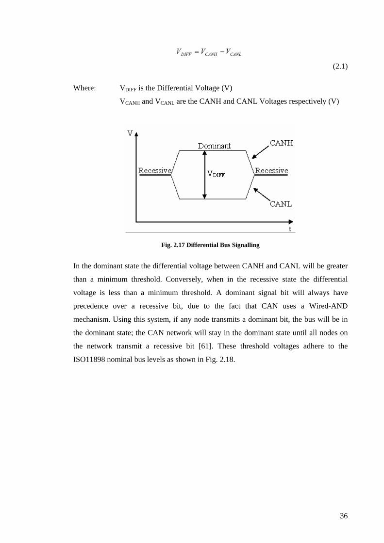
36
CANLCANHDIFF VVV −=
(2.1)
Where: VDIFF is the Differential Voltage (V)
VCANH and VCANL are the CANH and CANL Voltages respectively (V)
Fig. 2.17 Differential Bus Signalling
In the dominant state the differential voltage between CANH and CANL will be greater
than a minimum threshold. Conversely, when in the recessive state the differential
voltage is less than a minimum threshold. A dominant signal bit will always have
precedence over a recessive bit, due to the fact that CAN uses a Wired-AND
mechanism. Using this system, if any node transmits a dominant bit, the bus will be in
the dominant state; the CAN network will stay in the dominant state until all nodes on
the network transmit a recessive bit [61]. These threshold voltages adhere to the
ISO11898 nominal bus levels as shown in Fig. 2.18.
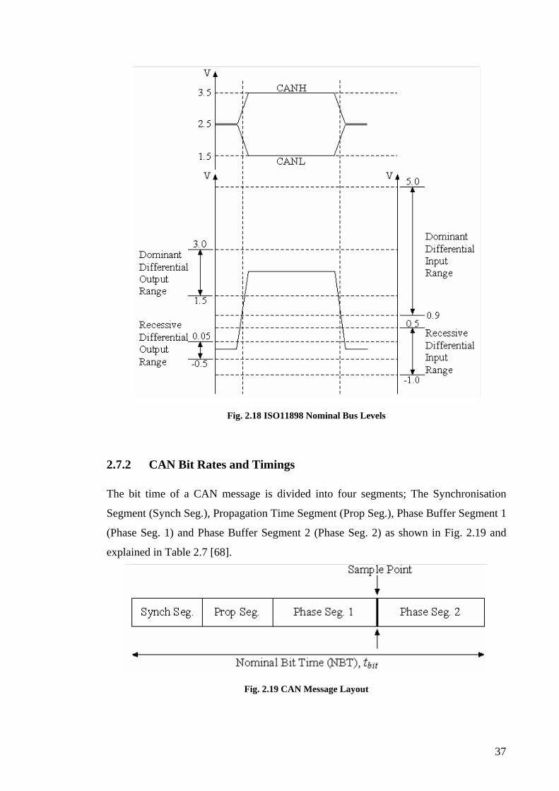
37
Fig. 2.18 ISO11898 Nominal Bus Levels
2.7.2 CAN Bit Rates and Timings The bit time of a CAN message is divided into four segments; The Synchronisation
Segment (Synch Seg.), Propagation Time Segment (Prop Seg.), Phase Buffer Segment 1
(Phase Seg. 1) and Phase Buffer Segment 2 (Phase Seg. 2) as shown in Fig. 2.19 and
explained in Table 2.7 [68].
Fig. 2.19 CAN Message Layout

38
Name Use Time Period (TQ)
Sync. Seg To synchronize the nodes on the bus. Bit edges are expected to occur within the Sync Seg.
1
Prop. Seg. To compensate for physical delays between nodes. Programmable : 1 - 8
Phase Seg.1 and
2
To compensate for edge phase errors on the bus. PS1 can be lengthened or PS2 can be shortened by resynchronisation
PS1- Programmable : 1 - 8 PS2- Programmable : 2 - 8
Table 2.7 Segments of a CAN Message
As illustrated in Fig. 2.19, the Nominal Bit Time (NBT), or tbit, is made up of the four
non-overlapping segments; therefore the NBT is the summation of the four segments
[69].
21 PSPSPropSegSynchSegbit ttttt +++=
(2.2)
Where: tbit is the bit period (seconds),
tSynchSeg is the synchronisation segment period (seconds),
tPropSeg is the propagation segment period (seconds),
tPS1 and tPS2 are the periods (seconds) for phase segment 1 and 2
respectively.
Each of the four segments are made up of integer units called Time Quanta (TQ). The
length of each Time Quantum is based on the oscillator period, with the base TQ
equalling twice the oscillator period. The TQ length equals one TQ clock period
(tBRPCLK), which is programmable using the Prescaler named the Baud Rate Prescaler
(BRP) [69], [68], as shown in the following equation (2.3).
OSCOSC F
BRP2TBRP2TQ *** ==
(2.3)

39
Where: TQ is the time quantum (seconds),
BRP is a user-configurable prescaler integer unit,
TOSC is the period of the oscillator used within a node (seconds),
FOSC is the frequency of the oscillator used within a node (Hertz).
The Nominal Bit Rate (NBR), which is the number of bits per second transmitted by an
ideal transmitter with no resynchronisation, can now be calculated using the following
equation (2.4).
bitbit t
1fNBR ==
(2.4)
Where: NBR is the nominal bit rate (seconds),
fbit is the frequency of a bit (hertz),
tbit is the bit period (seconds).
Developing Fig. 2.19 using the preceding equations, it can be seen that NBT can be
broken down further into a number of TQ. The Synch Seg. is always equal to 1 TQ
(Table 2.7) and the other three segments being the programmer’s choice depending on
the application and desired NBR, as shown in Fig. 2.20 [69].
Fig. 2.20 CAN Message in TQ
2.7.3 Propagation Delay As the CAN protocol is implemented to use a non destructive bit-wise arbitration
scheme, it is affected by propagation delays. If two nodes transmit their messages at the
same time, they must arbitrate for control of the bus, with the arbitration only being
effective if both nodes can sample the bit at the same time. Extreme propagation delays
will result in invalid arbitration. The propagation delay of a CAN system can be

40
calculated as being a signal’s round trip time on the physical bus, and is represented
mathematically as shown in the following equation (2.5) and illustrated in Fig. 2.21.
)(* drvcmpbusprop ttt2t ++=
(2.5)
Where tprop is the network propagation delay (seconds),
tbus is the time duration of a signal’s round-trip (seconds),
tcmp is the input comparator delay (seconds),
tdrv is the delay of the output driver (seconds).
Fig. 2.21 Propagation Delay between Nodes
2.7.4 Synchronisation In the CAN protocol, synchronisation occurs on the recessive to dominant edges and
their purpose is to control the distance between edges and sample points. The Phase
Buffer Segments (PS1 and PS2), along with the Synchronisation Jump Width (SJW) are
used to compensate for the oscillator tolerances. Both PS1 and PS2 may be lengthened
or shortened by synchronisation. There are two methods used for achieving and
maintaining synchronisation; Hard Synchronisation and Resynchronisation [68].
2.7.4.1 Hard Synchronisation
Hard Synchronisation only occurs on the first logic 1 to logic 0 (recessive to dominant)
edge during a bus idle condition. This represents a Start-of-Frame (SOF) condition.
Hard Synchronisation forces the edge to lie within the Synchronisation Segment by

41
causing the bit timing counter to reset to the Synchronisation Segment; hence,
synchronising all receivers to the transmitter. Hard Synchronisation only occurs once
during a message, and resynchronisation can not occur during the same bit time [68],
[70].
2.7.4.2 Resynchronisation Resynchronisation is implemented to maintain the synchronisation achieved by Hard
Synchronisation. Due to oscillator drift between nodes, the receiving nodes can lose
synchronisation if resynchronisation was not employed after Hard Synchronisation.
Resynchronisation is achieved by implementing a Digital Phase Lock Loop (DPLL)
function which compares the position of the expected edge (within the Sync Seg.) to the
actual position of a recessive-to-dominant edge on the bus. The DPLL will then adjust
the bit time as necessary. The SJW is used to compensate for any phase error by the
defined amount in resynchronisation. It is a value programmed by the user, in a range of
1 to 4 TQ, by which the bit period can be lengthened or shortened [68], [70], as shown
in Fig. 2.22.
Fig. 2.22 SJW used in Resynchronisation
2.7.5 CAN Message Framing
The CAN protocol defines 4 different types of data frames:
(i) Data Frame
(ii) Remote Frame
(iii) Overload Frame
(iv) Error Frame

42
2.7.5.1 Data Frame
As the data frame is the most commonly employed frame type, it will be discussed in
greater detail than the other three message frames. A Standard CAN data frame is
shown in Fig. 2.23.
Fig. 2.23 Standard CAN Data Frame
As illustrated in Fig. 2.23, the Standard CAN data frame consists of many different
fields; this is also true for the other three frame types. Each field is comprised of a
number of bits. The composition of the data frame is as describe below [59], [62], [64],
[66].
• Start of Frame Field – The SOF marks the beginning of the Data Frames and
the Remote Frames. It consists of a single ‘dominant’ bit.
• Arbitration Field – The Arbitration Field consists of the Identifier Field and the
Remote Transmission Request (RTR) Bit. The Identifier Field is 11bits in
length, and transmitted in order of ID10 to ID0. The seven most significant bits
(MSBs) (ID10 – ID4) must all not be ‘recessive’. For data frames, the RTR Bit
must be ‘dominant’, and for a Remote Frame the RTR Bit has to be ‘recessive’.

43
• Control Field – The Control Field consists of 6 bits. 4 bits are used for the Data
Length Code (DLC), which indicates the number of bytes in the Data Field, one
bit is for the IDE, while the last bit is reserved for future expansion.
• Data Field – The Data Field contains the data to be transmitted within the data
frame. It can contain 0 to 8 bytes, which are transferred MSB first.
• CRC Field – The CRC Field contains a cyclic redundancy check sequence,
along with the CRC Delimiter which is set to be a single ‘recessive’ bit.
• ACK Field – The ACK (Acknowledge) Field consists of two bits, one for the
ACK Slot and another for the ACK Delimiter. A transmitting node will send two
‘recessive’ bits, if a receiver receives the message correctly it will acknowledge
this by sending a ‘dominant’ bit in the ACK Slot back to the transmitter.
• End of Frame Field – The End of Frame Field consists of a sequence of seven
‘recessive’ bits.
The data frame described above is the Standard CAN Data Frame as outlined in the
CAN2.0A specifications. There has been a subsequent protocol release (CAN2.0B)
which describes the Extended Data Frame. The main difference between both frames is
that the Extended Data Frame has the capacity to support a twenty nine bit Identifier
Field as opposed to the Standard eleven bits. Thus the extended frame format offers a
greater ID range [62], [66].
2.7.5.2 Remote Frame Remote Frames are used to request information between nodes. A node which desires
information will transmit a Remote Frame on the CAN bus, on receiving the Remote
Frame the node which contains the desired data will then transmitted it on the CAN bus.
The Remote Frame’s composition is nearly identical to that of the Data Frame with the
only exceptions being that its RTR bit is ‘recessive’ along with its DLC being set to 0,
to indicate no data is being transmitted [62], [67].
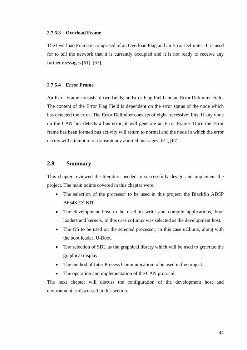
44
2.7.5.3 Overload Frame The Overload Frame is comprised of an Overload Flag and an Error Delimiter. It is used
for to tell the network that it is currently occupied and it is not ready to receive any
further messages [61], [67].
2.7.5.4 Error Frame An Error Frame consists of two fields; an Error Flag Field and an Error Delimiter Field.
The content of the Error Flag Field is dependent on the error status of the node which
has detected the error. The Error Delimiter consists of eight ‘recessive’ bits. If any node
on the CAN bus detects a bus error, it will generate an Error Frame. Once the Error
frame has been formed bus activity will return to normal and the node in which the error
occurs will attempt to re-transmit any aborted messages [61], [67].
2.8 Summary This chapter reviewed the literature needed to successfully design and implement the
project. The main points covered in this chapter were:
• The selection of the processor to be used in this project, the Blackfin ADSP
BF548 EZ-KIT
• The development host to be used to write and compile applications, boot
loaders and kernels. In this case coLinux was selected as the development host.
• The OS to be used on the selected processor, in this case uClinux, along with
the boot loader, U-Boot.
• The selection of SDL as the graphical library which will be used to generate the
graphical display.
• The method of Inter Process Communication to be used in the project.
• The operation and implementation of the CAN protocol.
The next chapter will discuss the configuration of the development host and
environment as discussed in this section.

45
3 System Configuration and Design

46
3.1 Introduction This chapter details the configuration and design of the complete system. All choices
made and methods used were based on the findings from the literature review. To
explain the system’s configuration and design process undertaken for this study the
chapter is divided into the following sections:
• Section 3.2 illustrates the configured system. It introduces all of the individual
components needed. These components will be explained in further detail in the
following sections.
• Section 3.3 outlines the configuration of the development host, coLinux. This
section describes the steps needed to install and configure coLinux, such that it
can be used to develop and compile U-boot, the uClinux kernel and any
application code for the BF548.
• Section 3.4 describes the compilation and porting of the boot loader, U-Boot and
also details the saving of U-Boot to flash memory.
• Section 3.5 covers the compiling and porting of the evaluation boards OS,
uClinux. The configuration of the uClinux kernel is also covered and describes
the inclusion and exclusion of functionality in the kernel.
• Section 3.6 outlines the configuration and modification of the CAN drivers, as
well as testing of sample code. It describes the problems encountered and
solutions faced while designing the CAN software on the BF548.
• Section 3.7 details the design principles for the graphical display used in the
project. It covers the design principles and development of basic SDL code,
along with the testing of this code.
• Section 3.8 outlines the method used for Inter Process Communications in the
project. It details the initial development and testing of the Named Pipes.
• Section 3.9 provides a summary of information presented in this chapter.

47
3.2 System Configuration Overview This chapter describes the configuration of the development host (PC) and evaluation
board (BF548). A complete overview of the system is shown in Fig. 3.1. Each section of
the diagram will be explained in more detail in the following sections.
Fig. 3.1 System Configuration Overview
3.3 coLinux When developing software for a uClinux based project, a Linux development host is
required. This development host is used to compile the boot loader (U-Boot), the
board’s OS (uClinux) and any applications that are run on the BF548. coLinux was
chosen as the development host for the project, as it can operate on top of a Windows

48
OS, and hence a full Linux box was not needed. The installation and configuring of
coLinux will be explained in the next section.
3.3.1 Installing coLinux The Debian version of coLinux was used in the project. The Debian installer file was
downloaded from the Blackfin website [71]. When the installer file was run on the
Windows machine, it set up a one gigabyte (1GB) partition that was then used for all
coLinux files. When the installation was complete, the partition contained all of the
standard directories associated with any Linux machine. Finally a batch file was written
to create a Windows shortcut for coLinux.
3.3.2 Configuring coLinux coLinux had to be configured such that the Windows partition and the coLinux partition
could communicate with each other. This was achieved by configuring a network
connection such that coLinux could use the Windows Ethernet network connection for
downloading new packages, and also for transferring files between both operating
systems.
3.3.2.1 Configuring the Network During the installation of coLinux, a TAP interface was automatically created in the
network connections folder of Windows. It is this interface that is used to connect both
the coLinux and the Windows OSs to the Ethernet. To allow connections, the Windows
Ethernet connection had to be shared as shown in Fig. 3.2 [72].

49
Fig. 3.2 Sharing Ethernet Connection
This TAP interface was configured to have an IP address of 192.168.0.1 and a subnet
mask of 255.255.255.0 as shown in Fig. 3.3.
Fig. 3.3 Configuring the coLinux TAP Interface
The Windows side of the network configuration was now complete. To configure the
network on coLinux the resolv.conf and interfaces files had to be edited to include the
IP address, subnet mask, gateway IP and the name server [73]. The interfaces file was
edited to contain the information shown in Table 3.1 and edited interfaces file is shown
in Fig. 3.4.
.

50
Name Address IP Address 192.168.0.100 Gateway IP 192.168.0.1 Subnet Mask 255.255.255.0
Table 3.1 coLinux Network Configurations
Fig. 3.4 Edited coLinux Interfaces File
When editing the resolv.conf file, the IP address set for the TAP interface is set as the
name server as shown in Fig. 3.5.
Fig. 3.5 Edited coLinux Resolv.conf File
coLinux was now configured to connect to the Ethernet. To test these connections ping
was used as shown in Fig. 3.6 and Fig. 3.7.

51
Fig. 3.6 Pinging coLinux from Windows
Fig. 3.7 Pinging Windows from coLinux
Finally communications between coLinux and the World Wide Web were verified by
using the “apt-get update” command. This command connects to the Web and updates
any coLinux packages that are not the latest revision. The web addresses which are used
for the updates were configured during the installation of coLinux. When the command
was run, each package currently installed in coLinux was checked and updated if a
newer version was available; hence proving that coLinux connected to the web. With
coLinux and Windows communicating, a method was needed to transfer files between
both OSs. This was accomplished using an FTP (File Transfer Protocol) server.
3.3.2.2 Configuring the FTP server The FTP server used in the project was Serv-U. This server was downloaded and
configured such that a folder called FTP Documents was created on the Windows OS.
This folder was the used to send and receive files from coLinux. As the folder was

52
situated on the Windows OS, the Domain IP of the server had to be set to the IP address
of the Windows OS, 10.9.100.134. The configured server is shown in Fig. 3.8.
Fig. 3.8 Configured FTP Server
To send and receive files from coLinux, the command “ftp 10.9.100.134” is used to log
on to the server. The user is asked to enter a username and password, once these are
entered properly, the user can receive files from the folder in the Windows environment
using the “get filename” command. To send files from coLinux to Windows the “put
filename” command is used. With the FTP server functioning correctly, full
communications were established between coLinux and Windows. Next the Blackfin
toolchains had to be installed in coLinux.
3.3.2.3 Installing the Blackfin Toolchains The Blackfin toolchains contain all the necessary library files and cross compilers
needed to compile code that is to be run on a Blackfin BF548 board, including U-Boot,
uClinux and any application programmes. There are two toolchains which need to be
installed, blackfin-uclinux and blackfin-linux-uclibc. Both of these toolchains were
downloaded from the Blackfin website [74]. The rpm (RPM Package Manager) versions

53
of the toolchains were downloaded to coLinux and were installed using the “alien –i
filename” command [18].
With the toolchains installed in coLinux, the path had to be edited such that it includes
the Blackfin toolchains. The path is used while compiling any code, to point to the
appropriate cross compiler, i.e. if compiling a uClinux kernel, without editing the path
to include the appropriate cross compilers, an error will be received. To edit the path the
following command is used;
“export PATH=$PATH:/opt/uClinux/bfin-uclinux/bin:/opt/uClinux/bfin-linux-
uclibc/bin”
With the path edited to include the Blackfin toolchains, coLinux can now be used to
compile programmes to run on the BF548. As a boot loader is needed to boot the
uClinux kernel on the board, U-Boot had to be compiled first.
3.4 U-Boot
U-Boot is the boot loader used when running uClinux on a Blackfin platform. Its job is
to point the CPU to the starting address of the OS, in this case a uClinux Kernel. To
accomplish this, the latest version of U-Boot was compiled and then saved into flash
memory such that it will run every time the BF548 board is powered up. When
compiling and porting U-Boot to the BF548, the steps given by Blackfin were closely
followed [18].
3.4.1 Compiling U-Boot To compile U-Boot the Blackfin toolchains must be installed in the development host,
coLinux, as stated earlier. The latest version of U-Boot was downloaded and
uncompressed using the command, “tar jxf U-Boot-1.1.6-2008R1.tar.bz2”. This
command will unpack U-Boot and put it into a directory with the same name, i.e. the
directory U-Boot-1.1.6-2008R1 will be created in coLinux. With the source code
installed in coLinux, U-Boot was then compiled.

54
3.4.1.1 Compiling U-Boot for Loading over the UART As the compiled version of U-Boot was to be loaded to the BF548 using the UART, this
had to be set in the header file for the device. To accomplish this, the Blackfin boot
mode must be set to Blackfin boot UART in the BF548-ezkit header file, as shown
below [18]. This edited header file is shown in Fig. 3.9.
#define BFIN_BOOT_MODE BFIN_BOOT_UART
Fig. 3.9 Setting Boot Mode to UART
After setting the boot mode to UART in the header file, the edited configuration file had
to be compiled for the changes to take affect. The command “make bf548-ezkit_config”
was used to compile the configuration file, as shown in Fig. 3.10.
Fig. 3.10 Configuring and Compiling U-Boot

55
Once U-Boot has compiled successfully the following files are created in the U-Boot
directory, as shown in Table 3.2.
File Description u-boot Compiled ELF image u-boot.bin u-boot converted to a raw binary u-boot.hex u-boot.bin converted to Intel Hex format u-boot.srec u-boot.bin converted to Motorola S-records format u-boot.ldr u-boot converted to Blackfin Loader format u-boot.ldr.hex u-boot.ldr converted to Intel Hex format u-boot.ldr.srec u-boot.ldr converted to Motorola S-records format
Table 3.2 Created Files from U-Boot Compilation
U-Boot was loaded on the BF548 using a UART loader (LdrViewer), and the file
required was “u-boot-ldr”.
3.4.2 Loading U-Boot onto the BF548 LdrViewer was used to load U-Boot, through the UART to the BF548 evaluation board.
This was achieved by connecting an RS232 cable from COM1 on the development
machine to the BF548 board and setting switch 1 on the BF548 to 7 (UART boot). The
U-Boot file (u-boot-ldr) was then opened and both the baud rate and com port were set
in LdrViewer. The port was then tested using the “test port” button as shown in Fig.
3.11.
Fig. 3.11 Configuring LdrViewer

56
When testing the port, if the message highlighted in Fig. 3.11 is received then the
LdrViewer can successfully talk to the port. The “Autobaud” button was then used to
test the connections between LdrViewer and the BF548 as shown in Fig. 3.12.
Fig. 3.12 Testing Communications between LdrViewer and BF548
If the message highlighted in Fig. 3.12 is received after running the “Autobaud”, the
BF548 is ready to receive the U-Boot file over the UART. This was achieved by
pressing the “Send DXE” button. When the U-Boot file had been successfully sent, the
feedback from the target was displayed in LdrViewer as shown in Fig. 3.13.
Fig. 3.13 U-Boot Transferred Successfully

57
3.4.3 Saving U-Boot to Flash When storing U-Boot into the flash memory, it was written into the serial flash on the
BF548. However when booting from flash, the boot mode will be set SPI boot. This
meant that U-Boot had to be recompiled, this time setting the boot mode to be SPI. To
accomplish this, the BF548 U-Boot header had to be edited as shown below. With the
following line replacing the previous boot mode, U-Boot was recompiled and ported to
the BF548 as explained above.
#define BFIN_BOOT_MODE BFIN_BOOT_SPI_MASTER
This new version of U-Boot was then written into the serial flash, giving the BF548 the
capabilities to boot from flash. When writing to the flash the following command was
entered into the virtual console (HyperTerminal) when connected to the board [18].
eeprom write 0x1000000 0 $(filesize)
The command above writes U-Boot into the serial flash of the board at address
0x1000000. When using the command the variable filesize will be replaced by the
actual size of the U-Boot file. The boot mode switch (switch 1) was then set to 3 (SPI
boot mode) and the board was reset. Now and every time the board is reset, U-Boot will
run automatically from the serial flash.
3.4.4 Configuring the Network Settings in U-Boot U-Boot is used to boot the uClinux kernel, which for this project was stored on the
development host. U-Boot will have to be able to connect to Ethernet so that it can port
the uClinux kernel from the development host. To configure the network settings on the
BF548, the network settings of the development host had to be established. These
settings were established using the command “ipconfig” in DOS, Fig. 3.14.

58
Fig. 3.14 Network Configuration of Development Host
From Fig. 3.14 it can be seen that the development host’s IP address is 10.9.100.134. As
the development host is used as a server for the board to port the uClinux kernel from,
this address was used for the server IP. The default gateway, 10.9.251.251, was used by
the board to connect to the network; hence this will be used for the gateway IP. Lastly
the board itself must be given an IP address, as the address 10.9.100.89 was not being
used on the network; this was assigned to the board. These settings were applied to the
board by entering the following commands in U-Boot.
set serverip 10.9.100.134
set ipaddr 10.9.100.89
set gatewayip 10.9.251.251
These settings were then saved by writing their values into the U-Boot that is stored in
flash using the command “save;” as can be seen in Fig. 3.15.
Fig. 3.15 Configuring the Network in U-Boot

59
Now every time the BF548 is booted, these network configurations will be used, so that
U-Boot will be able to connect to the network.
3.4.5 Testing U-Boot To test U-Boot a pre-compiled version of a uClinux kernel (uImage) was downloaded
from the Blackfin website [76]. This uImage was then stored on the development host
so that U-Boot would be able to access it through the network. To port the uImage to
the board, the “tftp 0x1000000 uImage” command was used in U-Boot, where tftp is
the command used to transfer the file using ftp, 0x1000000 is the starting address in
RAM where the file is to be placed and uImage is the actual kernel. When the command
was entered, the following was displayed on the virtual console (Fig. 3.16).
Fig. 3.16 Downloading the uImage
When the uImage is downloaded, it can be then booted using the command “bootm”.
Fig. 3.17 shows that the uClinux kernel has booted successfully and therefore proves U-
Boot is functioning correctly using the pre-compiled kernel. However, this pre-
compiled kernel does not have the desired functionality required for the project; hence a
new kernel has to be configured compiled using coLinux.

60
Fig. 3.17 Booted Kernel
3.5 The uClinux Kernel As the uClinux kernel contains a lot of different functionality, some of which was
required and some which was not, an optimum kernel had to be configured and
complied for use in this project.
3.5.1 Configuring and Compiling the uClinux Kernel The latest version of uClinux for the BF548 was downloaded from the Blackfin website
[76]. This source code was unpacked in coLinux using the “tar” command as explained
earlier. To configure the uClinux kernel to be compiled, the “make menuconfig”
command was used in coLinux whilst inside the uClinux directory. This command runs
a menu script; this menu script is then used to configure the uClinux kernel, as shown in
Fig. 3.18.
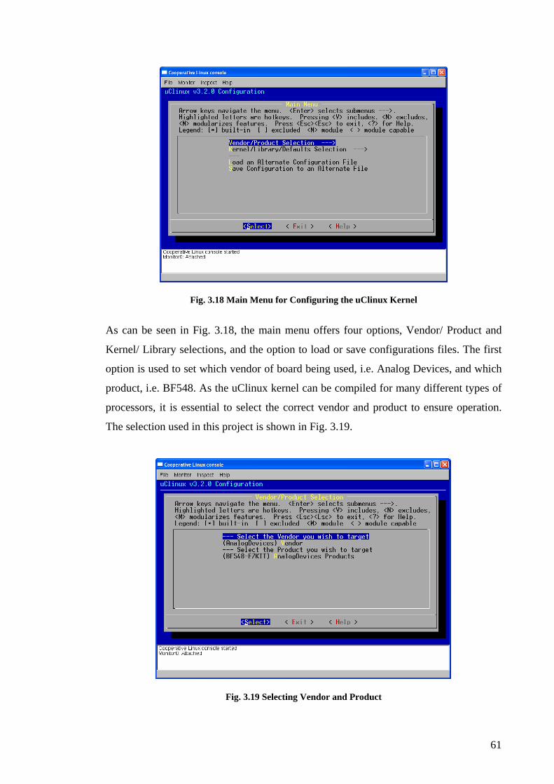
61
Fig. 3.18 Main Menu for Configuring the uClinux Kernel
As can be seen in Fig. 3.18, the main menu offers four options, Vendor/ Product and
Kernel/ Library selections, and the option to load or save configurations files. The first
option is used to set which vendor of board being used, i.e. Analog Devices, and which
product, i.e. BF548. As the uClinux kernel can be compiled for many different types of
processors, it is essential to select the correct vendor and product to ensure operation.
The selection used in this project is shown in Fig. 3.19.
Fig. 3.19 Selecting Vendor and Product
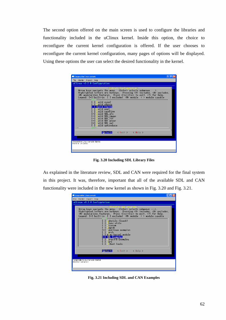
62
The second option offered on the main screen is used to configure the libraries and
functionality included in the uClinux kernel. Inside this option, the choice to
reconfigure the current kernel configuration is offered. If the user chooses to
reconfigure the current kernel configuration, many pages of options will be displayed.
Using these options the user can select the desired functionality in the kernel.
Fig. 3.20 Including SDL Library Files
As explained in the literature review, SDL and CAN were required for the final system
in this project. It was, therefore, important that all of the available SDL and CAN
functionality were included in the new kernel as shown in Fig. 3.20 and Fig. 3.21.
Fig. 3.21 Including SDL and CAN Examples

63
After including all desired functionality, the new configuration was then saved and the
“make” command is used to compile the new uClinux kernel as shown in Fig. 3.22.
Fig. 3.22 Compiling New Kernel
Once the kernel has compiled successfully, a new directory is created inside the uClinux
directory. The new directory was named “images” and contained the newly compiled
uClinux kernel (uImage). This uImage was then ported to the board and booted using U-
Boot as before. With the new uClinux kernel running on the BF548 board a simple
“hello world” program was used to test the new kernel’s functionality.
3.5.2 Testing the new uClinux Kernel The code for the “hello world” program was written in ‘C’. This program was compiled
and ported to the BF548. After porting the program to the board, its permissions had to
be changed, such that the OS has permission to execute the file. To achieve this, the
command “chmod 777 hello_world_test” is used. The chmod (change mode) command
is used to change the access permissions of the file, 777 is a numerical way of settings
all users’ access rights to read, write and execute. The hello_world_test is the name of
the compiled file.
After changing the access rights of the file, it was then run using the
“./hello_world_test” command. When the program was run, its displayed “Hello

64
World!!” on the virtual console and hence proved that the new kernel was functioning
properly, as seen in Fig. 3.23. After successfully testing the new uClinux kernel on the
board, other programmes were then developed to run on the BF548 to check full
functionality.
Fig. 3.23 Running Hello World Test Program
3.6 CAN Functionality The design and operation of the CAN program for this project, included editing the
drivers in the kernel for the successful operation on the board. This is explained in the
next sections.
3.6.1 Initial CAN Setup The BF548 contains two CAN ports (CAN0 and CAN1); which are used to connect the
board to an external CAN network. To access these ports, their drivers were included in
the compiled uClinux kernel. As stated earlier, the BF548 board was the latest
generation of Blackfin boards and therefore all of its functionality had not been fully
tested. This became apparent when the CAN drivers failed to initialise the CAN ports.
This lead to the CAN driver files being edited. It transpired that the kconfig file did not
include the BF548 which lead to there been no CAN drivers included in this processor’s

65
kernel. Investigating the kconfig file, it was noticed that the file contained three
different Blackfin model numbers, none of which were the BF548 as shown below.
depends on CAN4LINUX && EMBEDDED && (BF534 || BF536 ||
BF537)
This observation was then passed back to Blackfin and it was discovered that the BF548
CAN driver was not actually included in the new kernel. Blackfin suggested making the
following edits to the kconfig file of the CAN driver [58].
depends on CAN4LINUX && EMBEDDED && (BF534 || BF536 ||
BF537 || BF548)
After this change was made the driver was now available in the BF548 configuration
file as shown below.
Character devices ---> CAN, the car bus and industrial fieldbus ---> [*] can4linux support, the car bus and industrial fieldbus <M> Analog Devices BlackFin CAN Controller Note: The <M> means the driver will be a module in the kernel
With the “Analog Devices BlackFin CAN Controller” driver selected, the kernel was
recompiled. During this compilation different errors were encountered. These errors
were associated with one of the Blackfin CAN C programs (core.c). After investigating
the program file it was noticed that the section for the BF548 looked incomplete and the
missing values were consistent with the errors received. These results were passed to a
moderator of the Blackfin website, who implemented the required changes such that the
driver would work for the BF548.
3.6.1.1 Activating the CAN Driver As the CAN driver is a module driver, it has to be loaded into the kernel. To do this the
kernel must first be fully booted, and then the command “modprobe can” is used.
Where “modprobe” is a program used to add and remove modules from the uClinux

66
Kernel [18]. After entering the command the CAN driver was activated and the
confirmation of this was shown on the virtual console, Fig. 3.24. With this the CAN on
the BF548 was ready for initial testing.
Fig. 3.24 Activating the CAN driver
3.6.2 Initial Testing CAN sample code, with a baud rate of 125kbps, was provided in the uClinux kernel and
was used to test the CAN communications between the BF548 and a mikroElektronica
EasyPIC 4 board. On initial testing it was found that no communication was achieved
between both devices. CANalyzer, the automotive industries standard tool for CAN
network development and analysis, was used to monitor the traffic on the CAN bus. It
was first connected to the EasyPIC 4 board at the specified baud rate (125kbps) and
communications without errors was achieved. When CANalyzer was connected to the
BF548 at the specified baud rate, error messages were detected on the CAN bus, Fig.
3.25.

67
Fig. 3.25 Error Frames at 125kbaud
It was believed that these errors were due to the baud rate setting on the BF548 being
incorrect.
3.6.2.1 Baud Rate Error The bus between the BF548 and CANalyzer was probed using an oscilloscope to look at
the signal voltage and frequency, as seen in Fig. 3.26.
Fig. 3.26 CAN signal from BF548
With the value of the time period of the CAN signal determined to be approximately
7.5µs, the value of frequency was then calculated.

68
133.33Kbps7.5*10
1T1f 6 === −
(3.1)
Setting the baud rate on CANalyzer to the calculated frequency, 133kbps, allowed
communications without errors between the two devices, Fig. 3.27.
Fig. 3.27 CAN RX at 133kbps
3.6.2.2 CAN Header Files With the baud rate established to around 133kbps and not the desired 125kbps, the CAN
header files for the BF548 were checked to ensure that the CAN variables were set to
the correct values. The section of code which configured the CAN for 125kbps was
found at line 480 of the header file.
#if CAN_SYSCLK == 125 {----- lines cut -----}
#define CAN_BRP_125K 49 #define CAN_TSEG_125K 0x002f
From the code above it can be seen that the BRP (Baud Rate Prescaler) is set to 49, also
it can be seen that the value for TSEG is set to 0x002f. This hex number breaks down as
follows,
TSEG2 TSEG1
TSEG = 0x 0 0 2 F

69
The hex number above, shows that the value of TSEG2 is 0x2 (210) and the value of
TSEG1 is 0xF (1510). With these two values and the value of the propagation segment,
which was set in the header file, the value of the NTQ (Number of Time Quanta) was
established.
NTQ = prop_seg + TSEG1 + TSEG2
(3.2) = 3 + 15 + 2
= 20
Using the information ascertained from above and a system clock (SCLK) of 125MHz,
as stated in product documentation, the baud rate was found as follows.
)*)(( NTQ1BRPSCLKRateBaud+
=
(3.3)
Baud Rate = 20)*(5010*125 6
Baud Rate = 125kbps
From above, the settings in the CAN configuration file should warrant the desired baud
rate. Also from the header file, the values of the BRP and NTQ are known to be correct.
From this information, it can be seen that the only variable not confirmed, and would
cause the baud rate to be incorrect, is the system clock. Therefore the system clock must
not be operating at 125MHz.
3.6.2.3 Editing the System Clock Once it was discovered that SCLK was not running at the desired speed and after
researching the Blackfin site yielded no answers, a post was placed on the Blackfin
website [58]. From the replies received, it was discovered that the clock might have not
been set correctly in the kernel. The easiest fix for this was to edit the system clock on
boot up such that each time the kernel boots it sets all its clocks to 125Mhz, this in turn
will set the correct baud rate. To do this, changes had to be made to the kernel

70
configuration file. The system clock is determined using the following equation (3.4),
[18].
DIVSCLK
MULTVCO2
CLKIN(( SCLK
CLKIN_HALF
_
)_*)=
(3.4)
4
)20*)10*250
6
2((
SCLK =
4500*10 SCLK
6
= =125*106
SCLK=125MHz
Where: CLKIN - The clock input frequency
CLKIN_HALF - Cut input frequency in half
VCO_MULT - Clock input multiplier
CCLK_DIV - Core clock divider
SCLK_DIV - System clock divider
Note: CLKIN_HALF can only be 1 or 0.
Once the changes were made in the kernel configuration file, it was recompiled and
downloaded to the BF548. When the new kernel was booted, it froze. The kernel was
recompiled, downloaded and booted once more yielding the same result but eliminating
compilation errors. On researching this new issue it was discovered that the kernel
version (2008R1) used contained a bug which caused the kernel to freeze while re-
programming the clocks on boot-up.
This left two possible options;
(i) Upgrade to the latest kernel release
(ii) Edit the system clock in the current kernel

71
Careful deliberation resulted in the use of the second option, with a major factor being
all previous development in the project to this time had worked with the current version
of the kernel, and the newer kernel might involve newer problems.
There were two possible options in which to achieve the desired CAN baud rate;
(i) Change the clock in U-Boot and recompile it, so that it sets the system clock to
125MHz.
(ii) Edit the kernel’s CAN header files so that it could take the current system
clock and manipulate it to get the desired 125kbps baud rate.
It was decided that the second option would be the best, as all previous development
had been working fine in the current kernel, and changing the system clock in U-Boot
might lead to other problems. This option offered the benefits of a deeper understanding
of CAN in uClinux.
To edit the CAN header files, the actual system clock frequency was required. This was
established by checking the parameters in U-Boot. These parameters were stored in the
BF548 U-Boot header file and were used in the following equation (3.5) to calculate the
actual system clock.
DIVSCLK
MULTVCO2
CLKIN(( SCLK
CLKIN_HALF
_
)_*)=
(3.5)
4
)21*)10*250
6
2((
SCLK =
4*105 SCLK
625= =131.25*106
SCLK=131.25MHz

72
With the correct value of the system clock, equation 3.3 can now be used to find the
value of the CAN baud rate.
*NTQ)1((BRPSCLKBaudrate
)+=
(3.6)
2))151)*(3((49131.25*106
+++=
50*20131.25*106
=
= 131.25kbps
From above it can be seen that CAN was actually running at 131.25kbps instead the
desired 125kbps. With the value of the system clock at 131.25MHz and the desired
CAN baud rate of 125kbps. Using these values, and using the initial value of BRP (49),
as set in the CAN header file, then the value for NTQ can be established.
1)*NTQ)((49131.25*10 125*10
63
+=
(3.7)
(50*NTQ)131.25*10 125*10
63 =⇒
1050NTQ*50 =⇒
21NTQ =⇒
The desired NTQ was accomplished by setting TSEG1 = 15 and TSEG2 = 3 such that.
NTQ = 3 + 15 + 3
(3.8) 21 = 3 + 15 + 3
21 = 21
The value of TSEG_125K in the CAN header file was then set to 0x003F, instead of
0x002F as shown below.

73
#if CAN_SYSCLK == 125 {----- lines cut -----}
#define CAN_BRP_125K 49 #define CAN_TSEG_125K 0x003f The kernel was recompiled with the new edited header files and downloaded to the
evaluation board resulting in the CAN network running at the desired 125kbps. Fig.
3.28 shows the output from the BF548 CAN port when connected to CANalyzer
Fig. 3.28 CAN RX from BF548 at 125kbps
3.6.3 Testing CAN on the BF548
To test CAN on the BF548, the sample code inside the uClinux kernel was used. This
sample code contained two programmes;
(i) can_send – This program is used to send CAN messages from the BF548 and
has many different options for sending CAN messages.
(ii) receive – A program which is used to listen for CAN messages on the
network. If a CAN message is received, it is displayed in the
virtual console.
Each of the above programmes were tested individually and their results are explained
below.
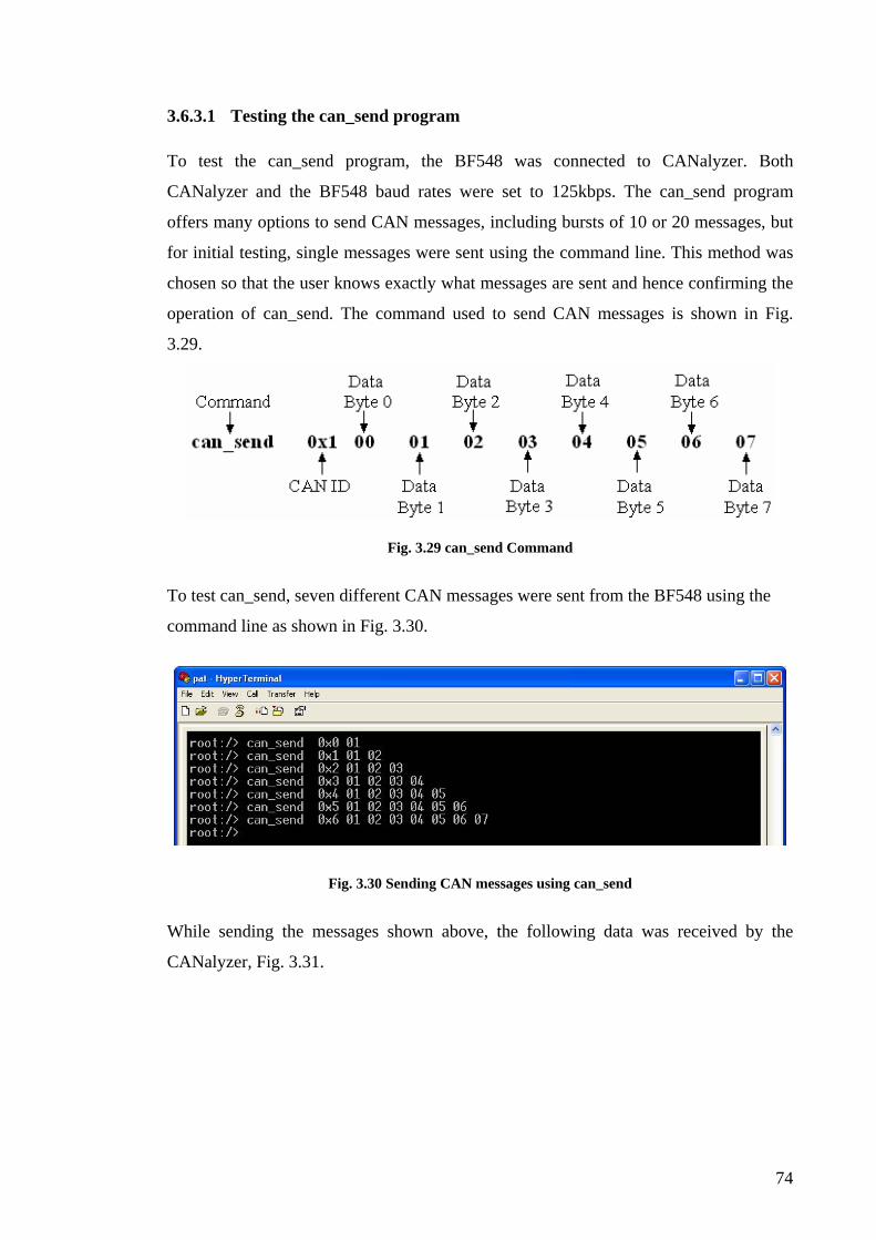
74
3.6.3.1 Testing the can_send program To test the can_send program, the BF548 was connected to CANalyzer. Both
CANalyzer and the BF548 baud rates were set to 125kbps. The can_send program
offers many options to send CAN messages, including bursts of 10 or 20 messages, but
for initial testing, single messages were sent using the command line. This method was
chosen so that the user knows exactly what messages are sent and hence confirming the
operation of can_send. The command used to send CAN messages is shown in Fig.
3.29.
Fig. 3.29 can_send Command
To test can_send, seven different CAN messages were sent from the BF548 using the
command line as shown in Fig. 3.30.
Fig. 3.30 Sending CAN messages using can_send
While sending the messages shown above, the following data was received by the
CANalyzer, Fig. 3.31.

75
Fig. 3.31 Messages received on CANalyzer
Fig. 3.31 shows that all CAN messages that were sent from the BF548 were transmitted
on the bus and received by CANalyzer correctly. The testing of the can_send program
was complete, and was proved that the CAN communication was working successfully.
3.6.3.2 Testing the receive program To test the receive program, both the BF548 and CANalyzer were connected and set to
125kbps. The receive program was then run on the BF548, whilst messages were
transmitted on the CAN network using CANalyzer. The receive program monitored the
CAN network and if any CAN messages were received, these were displayed on the
virtual console. An example of a typical display is shown in Fig. 3.32.
Fig. 3.32 Example of Received Message

76
The received messages comprises of six different parts;
(i) Received with ret – Used to signal if a message has been received. If a message is received with no errors this will equal 1, if there is errors it will equal -1
(ii) Receive time – Displays the board’s time stamp when the message
was received
(iii) CAN ID – Displays the CAN ID. The CAN ID for this program was displayed in decimal
(iv) Data Length – Displays the data length of the CAN message
(v) Data Bytes – Display the data contained in the CAN message, this
was displayed in hex
(vi) Flags – Displays flags associated with the CAN message
Fig. 3.33 Messages used to Test the Receive Program
To test the receive program, messages were sent using CANalyzer, as shown in Fig.
3.33, these were received by the BF548 and displayed on the virtual console, Fig. 3.34.
Fig. 3.34 Messages Received using receive program

77
All the messages sent using CANalyzer were received, with no errors, on the BF548.
With testing complete, an edited version of the receive program was used later in this
project. This edited program uses the data received in the CAN messages to change the
information displayed on the BF548’s LCD Panel (Implementation and Testing
chapter).
3.7 Simple Directmedia Layer Initial testing of the Simple Directmedia Layer (SDL) was performed using the SDL
software provided in the uClinux kernel.
3.7.1 Graphical Representations
The objective of this project was to create a flexible digital display, therefore it was
decided that two different forms of graphical representations would be used to display
information.
(i) A digital representation of a standard instrument display configuration. This
configuration contained two dials, a speedometer (speed) and a tachometer
(rpm).
(ii) A digital bar chart. This would display the speed in the form of a bar chart
along with any error messages that were ascertained from the CAN network.
During early development and testing of both SDL programs, a random number
generator was used to change both the speed and rpm. Both programmes were written
and tested individually. Later in the project, both programmes were combined with the
data from the CAN network being used to dictate the variables currently dictated by the
random number generator (see Implementation and Testing section).

78
3.7.2 Digital Representation of a Standard Dash Configuration The Digital Dash configuration was based on the analog dials used in the majority of
cars presently. This configuration contained both a speed dial and an rpm dial.
3.7.2.1 Graphics Creation The two dials were created using a graphics editor. However some considerations had to
be assessed before creating the graphics for the dash configuration. After researching
the available options, key decisions were made with the design layout such that:
(i) An image file would be created for each increment in speed or rpm for each
dial. This decision was made due to the heavy computational needs of SDL
to rotate an image. To overcome the amount of memory required to store all
the images, each image was stored as a PNG (Portable Network Graphics)
file, which offers very good compression ratios when compared to other
standard image file types.
(ii) The speed dial would also be in a separate file to that of the rpm dial such
that one of each would be called by SDL, thus reducing the memory used to
store the files. If both dials were in the same image, then multiple versions of
the fixed speed with different rpm would be required and vice versa.
Once these decisions were made, the dials were then created. Each incremental image of
a dial was achieved by rotating the needle by one degree in the image editing software.
The following diagram is the image used to represent the speed at 0 mph, Fig. 3.35.
Fig. 3.35 Speed dial at 0 mph

79
The rpm dials were created such that they would be slightly smaller in size and also
using a different background colour. This was merely for variation on the screen. The
following diagram is the image used to represent rpm at 0 rpm, Fig. 3.36.
Fig. 3.36 rpm dial at 0 rpm
The SDL code called one image of each dial. Fig. 3.37 shows the display for a speed of
0 mph and rpm of 0 rpm.
Fig. 3.37 End users display
3.7.2.2 Initial SDL Code (Analog Dials) Initial SDL code was very basic and only included one dial, the speed dial at first. This
program used a for loop to go from 0mph to 5mph. The speed was set using a variable
in the for loop i.e. if the variable “i” is equal to zero then the speed displayed on the
screen was 0 mph. A flow chart for the program is shown in Fig. 3.38.

80
Fig. 3.38 Flow Chart of Basic SDL Dial program
To implement the flow chart above, the following code was used.
for (i=0;i<=5;i++)
{
sprintf(mph, "%d.png", i);
message1 = IMG_Load( mph );
apply_surface( 0, 0, message1, screen );
if( SDL_Flip( screen ) == -1 )
{
return 1;
}
SDL_delay(del);
SDL_FreeSurface( message1 );
}

81
The variable message1 is initialised as an SDL surface, the desired image is then loaded
into a variable. The 2nd line of the code places the string x.png into the variable mph,
where x is equal to the value of i, e.g. if i = 3, then 3.png is stored in the variable. It is
the variable mph which is then used to load the desired image. This image is then
applied to the screen surface, where the variable screen is an SDL surface which is set
to the dimensions of the actual screen on the BF548 evaluation board. The two zeros in
the “apply_surface” function, represent where the image is applied, pixel 0 horizontally
and pixel 0 vertically i.e. the top left hand corner of the screen. The “SDL_Flip”
function displays the image in memory onto the evaluation board’s screen. If this
returns “-1” then the code will exit. A delay was introduced when displaying each
image, such that the images do not change so abruptly that the human eye can not
distinguish each step of the needle. Lastly the surface is freed to facilitate the loading of
the next image into the variable message1.
3.7.2.3 Using a Random Number Generator to Vary the Speed As the speed will not vary linearly in reality, it was necessary to test the code using a
random number generator. The two major differences needed in the code when using a
random number generator are:
(i) As a random number generator will not vary linearly in a given direction, the
code requires the capability to both increase and decrease the speed displayed
relative to the previous number generated.
(ii) The code will have to increment/decrement the speed on the screen so that the
dial doesn’t just jump, for example, from 25mph to 12mph, hence the code
will have to include some form of stepping mechanism.
To overcome the issues explained above an “if else” statement was used to distinguish
the direction of the speed and is shown below.
mph_value = rand() % 140;
if(mph_value < last_mph)
{

82
last_mph = last_mph - 1;
}
else if (mph_value > last_mph)
{
last_mph = last_mph + 1;
}
sprintf(mph, "%d.png", last_mph);
The value of mph_value is set by the random number generator, where %140 sets 140
as its maximum value. The value of last_mph is initially set to zero. On the first
iteration of the loop, mph_value will always be greater than last_mph, so the speed will
increase, in steps of 1mph, until the value of last_mph equals that of mph_value. When
this occurs a new value will be generated for mph_value and depending on whether it is
greater or smaller than last_mph, the speed will either increase or decrease.
After fully testing the code used to display the speed dial, the same code was
implemented for the rpm dial. With both programmes running as desired independently,
the next step was to integrate both programmes into one.
3.7.2.4 Integrated Dial Code As SDL is a sequential language, the code needs to run such that each dial will rotate
concurrently rather than the speed dial running to completion, then the rpm dial running.
As seen in Fig. 3.39 the code still runs sequentially, however each needle will only
rotate one increment and then the next needle will rotate one increment, and so on.
When one needle has run to completion and the dial displays the desired information,
the other needle will then run constantly until it has completed. When both dials display
the information received from the random number generator, new values for the speed
and the rpm are then generated. Due to the delay between each needle rotation being so
diminutive, the human eye can not distinguish when one needle is rotating and the other
isn’t. This visually leads to concurrency in both the dials. To achieve this, a “do –
while” loop was used.

83
Fig. 3.39 Flow Chart for Integrated Dial Code

84
do{ if(rpm_finished != 1) { // Display rpm if(last_rpm == rpm_value) { rpm_finished = 1; } } if(mph_finished != 1) { // Display mph if(last_mph == mph_value) { mph_finished = 1; } } } while((rpm_finished != 1) || (mph_finished != 1));
The code uses two variables; mph_finished and rpm_finished, both of which are
initialised to zero. These variables were used to flag when the corresponding needle had
run to completion, i.e. when the mph dial displays the desired speed, mph_finished is
then set to 1. To accomplish this an “if” statement was used such that, if the variable
last_mph was equal to the variable mph_value, set by the random number generator,
then mph_finished is set. When this occurs the rpm needle will now rotate to completion
and hence set rpm_finished to 1. The ending expression for the “do-while” states that
when rpm_finished is set, OR (||) mph_finished is set then exit the loop. A truth table for
a logical OR is shown below, where A and B are inputs and X is the output.
A B X
0 0 0
0 1 1
1 0 1
1 1 1
Table 3.3 Logical OR Truth Table

85
The truth table above shows that only when both A and B are false, will X also be false.
This is the same principle in the code, only when rpm_finished is false and
mph_finished is false, will the ending expression be false and hence the code will exit
the “do-while” loop. In the code the ending expression states “rpm_finished != 1”, this
statement is always true (1) until the rpm needle has reached the desired rpm. When the
needle has run to completion it will then set rpm_finished to 1 and hence make the rpm
side of the ending expression false (0). When the mph needle has run to completion it
will do the same and set the ending expression to be false thus exit the “do-while” loop.
The dials code was now successfully running as desired using the random number
generator. This code was later used with CAN messages, so that the CAN message
varied the speed and rpm on the dials rather than the random number generator. This
will be discussed later in this document (Implementation and Testing chapter).
3.7.3 Digital Bar Chart Representation The digital bar chart contained both a bar chart that represented the speed and also an
error message area, which would display any faults transmitted on the CAN network.
The idea being, if there were no faults requiring the user’s attention then the dials
display would be used. However, if a fault was introduced then the screen would drop
its dials configuration (speed and rpm), and display just the speed using the bar chart
configuration with its error message area clearly displaying the fault. In this section all
testing was preformed using the bar chart and later in this document, testing will be
performed on the dials and bar chart combined (Implementation and Testing chapter).
3.7.3.1 Graphics Creation The approach used to create the bar chart in SDL was slightly different than that used
for the dials. The bar chart configuration required a background bar chart with tiny
coloured bars placed on top to represent the speed. An advantage of this approach is it
required a very small amount of memory to save the images as the coloured bars are
minute. By displaying the bar chart in this fashion it proved that there are many

86
different ways to program the display. The bar chart design used for the project can be
seen in Fig. 3.40.
Fig. 3.40 Bar Chart
It was decided that as the speed increased the bars on the display would change colour
such that;
(i) Any speed less than 70 mph was displayed in green (Fig. 3.41)
Fig. 3.41 Speed below 70mph
(ii) Any speed less than 100 mph but greater than 70 mph was displayed in yellow
(Fig. 3.42)
Fig. 3.42 Speed greater than 70mph and below 100mph
(iii) Any speed over 100 mph was displayed in red (Fig. 3.43)
Fig. 3.43 Speed greater than 100mph

87
To fill the bar chart the same coloured bar is placed multiple times over the background,
therefore instead of creating an image for each speed as in the dials code, only one red,
one green and one yellow bar was required. When displaying error messages it was
decided to place the error message in the same image as the background bar chart such
that, if an error was to be displayed it would be part of the background. Three different
errors were created for testing purposes and an example of one is shown in Fig. 3.44.
Fig. 3.44 Bar Chart with Error Message
3.7.3.2 Initial SDL Code (Bar Chart) Initial code written for the bar chart design, was used to prove that using one image as a
background and imposing another image on top to represent the speed was possible.
The implemented code was as follows.
message = IMG_Load( "green.PNG" );
background = IMG_Load( "basic_dial_black.PNG" );
//Apply the background to the screen
apply_surface( 0, 0, background, screen );
//Apply the message to the screen
apply_surface( 50, 122, message, screen );
apply_surface( 54, 122, message, screen );
apply_surface( 58, 122, message, screen );
apply_surface( 62, 122, message, screen );

88
The program code above loads two images, the bar chart (“background”) and the green
coloured bar (“message”). The background is placed at location 0, 0 of the screen (top
left hand corner) and then the green bar is placed in 4 different locations, each of which
are 4 pixel apart horizontally. This 4 pixels shift represents the distance between each
bar in the bar chart, as shown in Fig. 3.45.
Fig. 3.45 Output from Initial Code
The code implementation and testing above proved that it was possible to layer images
on top of other images in SDL.
3.7.3.3 Basic Bar Chart Code Initial development and testing of the bar chart used a “for” loop to vary the speed. The
“for” loop was used to vary the required number of bars to be displayed rather than each
mph increment i.e. due to the scale on the bar graph, each bar represents 1.6mph.
During initial testing the bar chart background with no error messages was used, these
will be introduced later in this section. The objective of the basic code was to increment
the speed from 0 bars to 5 bars, i.e. 8mph. A flow chart for the program is shown in Fig.
3.46.
When writing the program code it was decided that each time the speed was updated
and displayed on the bar chart, the background would also be reloaded. This was to
accommodate later error message development i.e. when errors are introduced, the code
will check for errors between increments/decrements of the speed. If an error occurs, the
background representing that particular error message would then be displayed. No
delay was introduced when reloading the background; therefore the human eye could
not observe this. Similarly when the speed is incrementing/decrementing each bar is
refreshed on the screen but again due to the refresh rate the human eye can not identify
this. A flowchart of the program code is shown in Fig. 3.46.

89
Fig. 3.46 Basic Bar Chart Flow Chart
The code used to implement the flow chart in Fig. 3.46 is shown below.
for (s=0;s<=5;s++)
{
background = IMG_Load( “bground.PNG” );
message1 = IMG_Load( "green.PNG" );
apply_surface( 0, 0, background, screen );
for (k=0;k<=s;k++)
{
90
apply_surface( j, 212, message1, screen );
j=j+4;
}
if( SDL_Flip( screen ) == -1 )
{
return 1;
}
SDL_Delay( del );
SDL_FreeSurface( message1 );
SDL_FreeSurface( background );
j = 56;
}
The code above contains two “for” loops. The first “for” loop was used to generate the
speed, and the second “for” loop was used to display the desired speed. The code uses
the variable k to count from 0 to the value of the variable s, which holds the value of the
desired speed. The value stored in k is the number of bars required to represent the
speed. Inside the loop the variable j is used to distinguish where each bar is to be placed
on the screen. j is initialised to 56, which is the starting point of the bar chart, and each
time a new bar is placed onto the screen, 4 is added to j such that the next bar will be
placed 4 pixels to the right of the last. This loop will then run until the value in k is
equal to that in s. When this occurs the code displays the desired speed and then delays
so that the eye can see the change in speed.
3.7.3.4 Changing the Bar Colour with Speed As mentioned earlier the bar chart design required different ranges of speeds to be
displayed with different coloured bars. To accomplish this, the change over values in
speed and bars was required. This information is represented in Table 3.4.
Bar Colour Green Yellow Red Speed (mph) 0 - 70 70 - 100 100 – 145 No. of Bars 0 - 41 42 - 59 59 – 88
Table 3.4 Change Over Values of Coloured Bars

91
With the information above, “if” statements were used in the code so that the colour of
the bars used to display the speed, changed for different ranges of speed. These
statements are shown below:
if ((s>=0) && (s<42))
{
//use green bars
}
else if ((s>=42) && (s<60))
{
//use yellow bars
}
else if ((s>=60) && (s<88))
{
//use red bars
}
The only additional change now needed to the basic code was to load the appropriate
coloured bar, i.e. change the image to be loaded (e.g. yellow.PNG or red.PNG) in the
following line of code:
message1 = IMG_Load( "green.PNG" );
3.7.3.5 Decrementing the Speed With the speed bars incrementing and changing bar colour as desired, the code would be
required to decrement the speed also. This was achieved by editing the basic code
previously discussed in this document to add the decrementing functionality. The
changes made to the code are shown below.
for (s=5;s>=0;s--)
{
background = IMG_Load( bground );
message1 = IMG_Load( "green.PNG" );

92
apply_surface( 0, 0, background, screen );
for (m=1;m<s;m++)
{
apply_surface( j, 212, message1, screen );
j=j+4;
}
The code above sets the initial speed to 5 and decrements to zero; it is the first “for”
loop, based on the variable s, which sets the speed. The second “for” loop, based on the
variable m, sets how many coloured bars are used to display the speed. Comparing this
loop to that used for incrementing the speed there is a slight change. The variable m
“for” loop sets the number of bars to be displayed; therefore if the loop used for
incrementing was the same as that for decrementing, then the actual speed displayed
would be two bars off the actual speed. To eliminate this problem, m was set equal to 1
rather than zero, and the loop was set to terminate when m is equal to s.
3.7.3.6 Using a Random Number Generator to Vary the Speed As speed does not vary linearly in a vehicle, it was necessary to test the code using a
random number generator. When using a random number generator the code must be
capable of increasing and decreasing the speed accordingly. This was accomplished as
shown in the flow chart in Fig. 3.47.

93
Fig. 3.47 Flow Chart for Bar Chart Representation of Speed

94
The flow chart illustrates that several conditions must be met before choosing which
function to run in the code. To accomplish this “if” statements were used and are shown
below:
if ((i>=0) && (i<42) && (t>i))
{
green_up;
}
else if ((i>=0) && (i<42) && (t<i))
{
green_down;
}
else if ((i>=42) && (i<60) && (t>i))
{
yellow_up;
}
else if ((i>=42) && (i<60) && (t<i))
{
yellow_down;
}
else if ((i>=60) && (i<88) && (t>i))
{
red_up;
}
else if ((i>=60) && (i<88) && (t<i))
{
red_down;
}
In the code the variable i represents the value last_speed and the variable t represents
the value new_speed.
else if ((i>=42) && (i<60) && (t>i))

95
The line of code above states, that if the last speed is greater than or equal to 42
(minimum value for the bar colour to be yellow) and less than 60 (maximum value for
the bar colour to be yellow), and if the new speed is greater than the last speed, then use
the function ‘yellow_up’. It can be seen in the last condition, if the new speed is greater
than the last speed displayed, then the number of bars must be incremented to display
the new speed. Also with the values falling inside the yellow range, the function
executed will be the ‘yellow_up’ function.
The “for” loop now had an added stipulation requiring it to perform the loop until the
correct speed is reached. The “for” loop below is taken from the ‘yellow_up’ function,
but each function has their own appropriate “for” loop.
for (s=i;((s<60)&&(s<t));s++)
The “for” loops inside the functions, use the variables set by the random number
generator. When the program enters a function, in this case ‘yellow_up’, it first sets the
variable s to the value of the last speed, this value of s can be anything from 42 to 60 as
the program is inside this particular function. Next the “for” loop checks that the last
speed is less than 60 (max. yellow value) and less than the new speed. To accomplish
this, a logical AND was used, for which a truth table is shown in Table 3.5, where A
and B are inputs and X is the output.
A B X
0 0 0
0 1 0
1 0 0
1 1 1
Table 3.5 Logical AND Truth Table
Using this in the “for” loop inside the condition, when the value of the variable s
increases above the maximum value of the yellow bars (60) then the first stipulation
(s<60) becomes false and hence the program exits this conditional statement. Also if the
value of the variable s is not less than the value of variable t, i.e. last speed is equal to

96
the new speed, then the code will also exit the function. Looking at the flow chart in
Fig. 3.47 it can be seen that if the value of last speed (variable s) is greater than the
maximum value for the yellow bars then the code will enter the ‘red_up’ function. Once
the value of last speed (variable s) is equal to that of the new speed (variable t), then the
random number generator will generate a new speed.
3.7.3.7 Displaying Error Messages with the Bar Chart With the bar chart displaying the speed as desired from the random number generator,
the last functional requirement to be met for the bar chart was to display error messages
on the screen. Using the random number generator to generate the speed, it was decided
to prompt the user to select the error message at the start of the program. This decision
was made due to only a small number of error message screens being created for testing
purposes. The code to select the error messages is shown below.
printf("Please select error (1-3)\n");
scanf("%d", &err);
sprintf(bground, "err%d.PNG", err);
printf("%s will be displayed as background\n",
bground);
The program code above prompts the user to select an error message between 1 and 3.
The value entered by the user is then initialised to an integer. This integer sets the
number of the error file, i.e. if the user enters the number 2, then the string err2.PNG
will be saved in the variable bground. A table of the error messages is shown in Table
3.6.
Filename Description
err1.PNG Basic Bar Chart with no errors
err2.PNG Back left tyre pressure low
err3.PNG ABS Failure
Table 3.6 Bar Chart Error Screens

97
When executing the code, the following was displayed on the virtual console.
Fig. 3.48 Users Prompt for Selecting Errors
From Fig. 3.48, the error selected was error 2; this in turn was displayed on the BF548’s
screen, as shown in Fig. 3.49.
Fig. 3.49 Background set as Error 2
The bar chart code was now producing the desired functionality using the random
number generator. This program code was then used with CAN messages, such that the
CAN message would vary the speed on the bar chart rather than the random number
generator and the CAN ID would set the error message to be displayed. This is
discussed later in this document (Implementation and Testing chapter).
3.8 Inter Process Communications The Inter Process Communications (IPC) used in this project is called Named Pipes,
which allows for communications between running processes in the uClinux kernel,
namely, the CAN and the SDL processes. When using pipes, one has to be able to write

98
to a pipe and read from the same pipe. This involves writing two different pieces of
code as explained below.
3.8.1 Writing to a Pipe As Named Pipes was used in the project the first thing that had to be accomplished was
to name and create the actual pipe used.
3.8.1.1 Naming and Creating a Pipe The name of the pipe is created by using a “#define” in C code. The name of the pipe
being used for the initial test was “RECFIFO”; receive FIFO (First In First Out). To
name the pipe, the following line of code was used:
#define RFIFO_FILE "RECFIFO"
The line above sets the name of RFIFO_FILE to be “RECFIFO”; this was then used to
create the Named Pipe, to name the actual pipe. To create the pipe the following line of
code was used:
mknod(RFIFO_FILE, S_IFIFO | 0666, 0);
To create a Named Pipe the mknod() function must be used. When using the mknod(),
three arguments have to be passed to the function; the first argument is the desired name
of the Named Pipe. As RFIFO_FILE is defined as the desired name for this pipe, it is
passed as the first argument. The second argument is the creation mode, in the example
above the second argument is “S_IFIFO | 0666”, this line tells the mknod() function to
create a Named Pipe (S_IFIFO) and sets the access permissions. In this case the access
permission is 0666 which sets all users permissions to read and write. The last argument
passed is a device number, as this is not used in Named Pipes it is set to zero [52].
99
3.8.1.2 Writing to the Created Pipe When writing to a pipe, data is required to be put into the pipe. Later in the project this
data was taken from the CAN network, but in the interim a simple string was used. To
create the string the following line of code was used.
char mes[] = "Hello World\n";
The line of code above sets up a string called mes containing “Hello World”. To write
the string to the pipe it first has to be opened.
fp = open(RFIFO_FILE, O_WRONLY);
The line above opens the pipe, RFIFO_FILE, and sets it to write only (O_WRONLY).
A third argument can be added to the code above, known as the non-blocking option
(O_NONBLOCK). This option allows the pipe to be opened for another write even if
the current data has not been read. This option was not desired in this case and was not
enabled in the code [52]. With the pipe open, it can be written to by using the following:
write(fp, mes, 12);
The write function above takes three arguments; firstly the file that the write function is
to write to, in this case this is fp, which is the opened pipe. The second argument is the
buffer the function has to write from; in this case the buffer will be the string mes. The
last argument is the number of bytes of data to be written from the buffer, in this case
12. Lastly the pipe must be closed; this accomplished using the following:
close(fp);
Since the non blocking option was not enabled, this pipe can not be opened again until
the data has been read from the pipe. This was desired for the project as it prevents any
data being lost.
Once the program was ported to the BF548, its access rights were changed to make the
program executable. The contents of the directory were then listed to show the write

100
program was on the evaluation board (wrpipes_test). The program was then run as
shown in Fig. 3.50.
Fig. 3.50 Running Write to Pipes code on BF548
When the program was executed, it created a pipe and wrote the string into it. The
program waited until the pipe was read from, and then exited. As of yet no code had
been written to read form the pipe. Instead the “cat” command was used to display the
contents of a file; in this case the Named Pipe (RECFIFO). To display the contents of
the Named Pipe the command “cat < RECFIFO” was used. The command was run on
PuTTY to display the contents of the pipe, as the write pipes program was still running
on the virtual console. The following was shown on the PuTTY screen, Fig. 3.51.
Fig. 3.51 Displaying the Contents of the Named Pipe
From Fig. 3.51, it can be seen that the pipe contained the string “Hello World”, which
was written to the pipe by the write to pipes program (wrpipes_test). This test proved
that the write to pipes program was working correctly. Next code had to be written to
read from a Named Pipe.
3.8.2 Reading from a Pipe Reading from a Named Pipe is less difficult than writing to a Named Pipe, but both
follow the same methodologies with the exception of a few minor steps. When reading
from a Named Pipe the pipes name has to be defined in the code as explained earlier.

101
No Named Pipe has to be created when reading, however, the Named Pipe must be
reopened. To open a Named Pipe for reading the following code is used.
fp1 = open(RFIFO_FILE, O_RDONLY);
This Named Pipe was now set to be read only (O_RDONLY) when opening and again it
can be seen that the non blocking option was not set, therefore the Named Pipe will be
in blocking mode. With the Named Pipe open, the program can now read the file. This
is accomplished using the following:
read(fp1, readbuf1, 12);
The line of code above read 12 bytes of data from the open pipe, fp1, and then placed
the data in the buffer readbuf1, which was initialised as an array of 12 characters. After
reading from the pipe, the pipe was again closed using the close function. Lastly, the
contents of readbuf1 were displayed to the user using:
printf("%s",readbuf1);
The code was compiled and ported, along with the write program (wrpipes_test) to the
BF548 and the access permission of both programmes were changed. The contents of
the directory were listed to show that both programmes were in the directory. The write
program (wrpipes_test) was then executed using the virtual console as shown in Fig.
3.52.
Fig. 3.52 Running Write program in conjunction with Read program
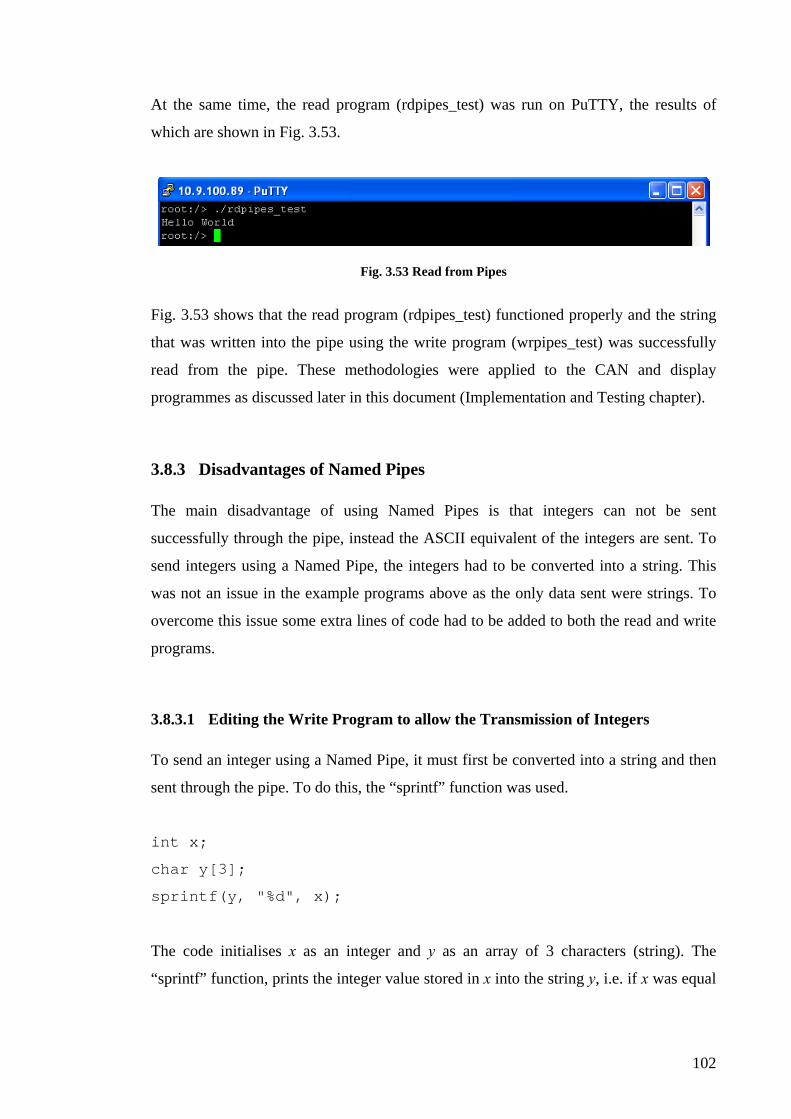
102
At the same time, the read program (rdpipes_test) was run on PuTTY, the results of
which are shown in Fig. 3.53.
Fig. 3.53 Read from Pipes
Fig. 3.53 shows that the read program (rdpipes_test) functioned properly and the string
that was written into the pipe using the write program (wrpipes_test) was successfully
read from the pipe. These methodologies were applied to the CAN and display
programmes as discussed later in this document (Implementation and Testing chapter).
3.8.3 Disadvantages of Named Pipes The main disadvantage of using Named Pipes is that integers can not be sent
successfully through the pipe, instead the ASCII equivalent of the integers are sent. To
send integers using a Named Pipe, the integers had to be converted into a string. This
was not an issue in the example programs above as the only data sent were strings. To
overcome this issue some extra lines of code had to be added to both the read and write
programs.
3.8.3.1 Editing the Write Program to allow the Transmission of Integers To send an integer using a Named Pipe, it must first be converted into a string and then
sent through the pipe. To do this, the “sprintf” function was used.
int x;
char y[3];
sprintf(y, "%d", x);
The code initialises x as an integer and y as an array of 3 characters (string). The
“sprintf” function, prints the integer value stored in x into the string y, i.e. if x was equal
103
to 10, then 10 would be stored in the form of a string in y. Therefore y will contain 10 in
string format. This format can now be sent using a Named Pipe.
3.8.4 Editing the Read Program to allow the Manipulation of Integers The read program does not need to be edited to receive the integers in the string format.
However the read program will only be able to display the integer in its string format.
The string format of an integer was not the desired format; therefore the read program
had to change the string version of the integer to an actual integer. This is accomplished
using following line of code.
t = atoi(y);
The variable t is initialised to be an integer. The line of code above uses the “atoi”
function to convert the string contained in y into an integer and then places into the
variable t.
3.8.5 Testing the Transmission and Reception of Integers To test the transmission and reception of integers using Named Pipes, the example code
used in sections 3.8.1 and 3.8.2 were edited.
3.8.5.1 Editing the Write Program The write program (wrpipes_test) was edited such that the user was prompted to enter
an integer between 0 and 100. This integer was then converted into a string and written
into the Named Pipe, RECFIFO, as shown below.
printf("Please enter a number between 0 and 100.\n");
scanf("%d", &i);
sprintf(mes, "%d", i);
fp = open(RFIFO_FILE, O_WRONLY);
write(fp, mes, 3);

104
close(fp);
The integer inputted by the user was stored in the variable i, which is then converted
into a string and written into the Named Pipe.
3.8.5.2 Editing the Read Program The read program (rdpipes_test) was also edited; such that the number the user entered
in the write program would be displayed on the virtual console. This was achieved using
the following:
fp1 = open(RFIFO_FILE, O_RDONLY);
read(fp1, readbuf1, 3);
close(fp1);
j = atoi(readbuf1);
printf("String: %s\n",readbuf1);
printf("Integer: %d\n",j);
This code reads the string from the Named Pipe, RECFIFO, and then stores it in the
variable readbuf1. The contents of readbuf1 is then converted into an integer and stored
in the variable j. The string, readbuf1, and the integer, j, were both displayed on the
virtual console to show the user that they were the same.
3.8.5.3 Running the Test Programmes After editing the write and read programmes both were run on the BF548 evaluation
board. The write program (wrpipes_int) was executed on the virtual console as shown
below, Fig. 3.54.

105
Fig. 3.54 User Prompt to enter Integer
As the write program was running on the virtual console, the read program (rdpipes_int)
was running on PuTTY as shown, Fig. 3.55.
Fig. 3.55 Output from Read Program
From Fig. 3.55, the number the user had entered in the write program i.e. 64, has been
successfully sent through the pipe and converted back into an integer.
3.9 Summary In this chapter the system design was taken from the problem definition and
requirements, to a final system design. This chapter reviewed the methods used and
choices made when configuring and designing the proposed system. The main points
covered in this chapter were:
• The configuration of the development host, coLinux, which was used to compile
all code that ran on the BF548.
• The compilation and porting of both U-Boot and uClinux to the evaluation
board.

106
• The changes made to the CAN driver for proper execution on the BF548, along
with the testing of the CAN sample code.
• The design of the display programmes in SDL, including the testing of the both
the Analog Display and the Bar Chart configurations.
• The design methods used for Named Pipes as the IPC for the system, which
included testing of basic Named Pipes programs.
The next chapter will discuss the implementation and testing of the final system using
the design processes discussed in this chapter.

107
4 System Implementation and Testing

108
4.1 Introduction This chapter outlines and explains all methods used during the system implementation
and testing stage of this study. The chapter is divided into the following sections:
• Section 4.2 outlines the methods used when implementing the CAN process for
the final system. This will include the manipulation of received data from the
CAN network and the addition of Named Pipes to the CAN code.
• Section 4.3 describes the methodologies applied when implementing the SDL
process in the final system. This included the integration of both SDL programs
explained earlier. Also IPC were added to the SDL code to allow
communications between the display and CAN processes
• Section 4.4 details the results found while testing the final system, and
comments on these results.
• Section 4.5 shows the results found from stress testing the final system, and
comments on these results.
• Section 4.6 provides a summary of information presented in this chapter.
4.2 CAN Implementation The sample code supplied with the uClinux kernel was used to receive data from a CAN
network. This code was edited such that the desired parts of the message would be
parsed from the CAN message and, using Named Pipes, be sent to the SDL code. This
sent data would then be manipulated and displayed on the BF548’s LCD screen.
4.2.1 CAN Message Breakdown The first step was to design the CAN message strategy to be used in conjunction with
the SDL code. After some research it was discovered that there were no set standards or
practices concerning CAN message data and the displaying of information. From this
research it was discovered that automotive manufacturers use different bytes of the
CAN message data to represent the speed, i.e. one manufacturer might use byte 4 and 5,
while another might use byte 1 and 2. With no standard to adhere too, the selection of

109
which bytes to use was completely the programmer’s choice. The data bytes chosen for
this project are shown in Fig. 4.1.
Fig. 4.1 Breakdown of CAN message
The CAN ID was used to configure the screen layout e.g. to display either the digital
dash or the bar chart configuration. The CAN ID would also set the error screen to be
displayed if the bar chart configuration was chosen. Both bytes 0 and 1 were used to
represent the speed and byte 2 was used to represent the rpm.
4.2.2 CAN Sample Code The CAN sample code (receive) provided in the uClinux kernel was used for CAN
communications between the BF548 and the CAN network. This code was already fully
tested as explained earlier (CAN design section). A flow diagram for the receive
program is shown in Fig. 4.2.
The receive program extracts both the CAN ID and the data length from the CAN
message. Using the data length, the program executes a “for” loop to obtain each data
byte from the received CAN message. When the variable i is equal to the data length, all
the data bytes have been extracted from the message and the code will then await the
next message.
Due to the layout of the code, it allows for easy extraction of the desired data for this
project. As the CAN ID is stored in its own variable, this variable can be used to write
the CAN ID into a Named Pipe. Likewise due to each data byte being stored in
individual variables, e.g. data byte 0 from the first received CAN Message will be
stored in the variable rx[0].data[0], this allows for the insertion of individual data bytes
into a Named Pipes with relative ease.

110
Using the information gained above, the CAN receive sample code was then edited to
add Named Pipes, so as to allow for Inter Process Communications (IPCs) between the
CAN program and the SDL program.
Fig. 4.2 Receive Flow Chart
4.2.3 Editing the Sample Code The CAN receive sample code had to be edited such that the values of the CAN ID, of
both byte 0 and 1 (speed) and byte 2 (rpm) be put into three different pipes IDFIFO,
SPEEDFIFO and RPMFIFO respectively. To accomplish this, the same methodology

111
used when developing the write to pipes program (wrpipes_test) was applied. A flow
chart for the edited receive program is shown in Fig. 4.3.
Fig. 4.3 Receive with Named Pipes Flow Chart

112
4.2.3.1 Creating the Named Pipes To add Named Pipes to the receive code; firstly the three pipes must be defined.
#define SPEEDFIFO_FILE "SPEEDFIFO"
#define IDFIFO_FILE "IDFIFO"
#define RPMFIFO_FILE "RPMFIFO"
The Named Pipes are then created using the mknod() function as explained earlier (see
IPC section).
mknod(SPEEDFIFO_FILE, S_IFIFO|0666, 0);
mknod(IDFIFO_FILE, S_IFIFO|0666, 0);
mknod(RPMFIFO_FILE, S_IFIFO|0666, 0);
With the Named Pipes created, the variables used to populate these must be developed.
4.2.3.2 Populating the Variables used when Writing to the Named Pipes The receive code required two “for” loops to obtain the CAN messages. The first “for”
loop is used to monitor the number of CAN messages received from the network, while,
the second monitored the data sent in each message. Both “for” loops are also used to
populate a 2D array. The first “for” loop uses the variable i as one coordinate of the
array. The variable i stores the number of messages received. The second “for” loop
uses j to count the data bytes from 0 to the data length for each message, for each
increment the value of the equivalent data byte is stored in the array location
rx[i].data[j]. An example of a 2D array is shown in Table 4.1. Looking at the table, it
can be seen that the value of data byte stored in rx[2].data[1] is 3, where 2 is the value
of i and 1 is the value of j.

113
Table 4.1 2D Array used in Receive Program
4.2.3.3 Populating the Variable used for the CAN ID The CAN ID array location was then used to populate the variable for the CAN ID; this
was accomplished using the code below.
sprintf(id, "%d", rx[i].id);
The line of code above, copies the value from the array location, rx[i].id, into the string
id. The i variable in the array rx[i].id distinguishes which CAN message the ID is taken
from, e.g. if the CAN message was the first received message then its ID would be
stored in rx[0].id. The CAN ID variable is now populated and ready to write to the
Named Pipe. Next the speed and the rpm variables must also be populated.
4.2.3.4 Populating the Speed Variable As mentioned earlier, the speed may be varied using two data bytes, data byte 0 and
data byte 1, as shown in Fig. 4.1. Therefore, a decision had to be made whether to send
each data byte through its own pipe, or to send both data bytes through one pipe. As the
SDL program will have to manipulate both data bytes mutually to display the speed, it
was decided that both would be sent using one pipe. Prior to writing the speed value to
the pipe, both bytes were combined to represent a single decimal value.
Due to the fact that both data bytes are in hex format, the decimal equivalent of each
data byte was obtained, and then added to give an overall decimal value. When
obtaining the decimal equivalent, the value of data byte 1 was seen as the least

114
significant bit (LSB) while the value of data byte 0 was seen as the most significant bit
(MSB). The following lines of code were used to accomplish this.
byte0 = ("%d", rx[i].data[0]);
byte1 = ("%d", rx[i].data[1]);
The code above, sets the value of byte 0 and byte 1 to be the decimal equivalent of the
hex numbers stored in the 2D array, rx[i].data[0] and rx[i].data[1] respectively. With the
decimal equivalent of each byte, the following line of code was used to establish their
combined value.
speed = byte0*pow(16,2) + byte1;
With the equivalent value calculated it is then stored in the variable, mes, which is
initialised as a string. This is accomplished using the line of code shown below.
sprintf(mes, "%d", speed);
With the CAN ID and speed variables populated, the rpm variable is the last to be
populated.
4.2.3.5 Populating the rpm Variable
As the rpm value is only one data byte of the CAN message, less manipulation is
required in comparison to the speed value. Firstly, the decimal value of data byte 2 had
to be obtained. This was achieved using the following line of code.
byte2 = ("%d", rx[i].data[2]);
With the value of data byte 2 obtained, the rpm variable was populated by using the
following line of code.
sprintf(rpm, "%d", byte2);

115
4.2.3.6 Writing the Populated Variables to their Named Pipes Once all three variables had been populated, they were copied to their equivalent
Named Pipes. This was accomplished using the same methodologies as explained
earlier (IPC section). The code used to write the CAN ID to the pipes is shown below.
fp1 = open(IDFIFO_FILE, O_WRONLY);
write(fp2, id, 10);
close(fp2);
printf("id = %s\n", id);
The code above is similar to that utilised in the IPC section. The only difference being
that after each variable is written to it’s pipe it is then displayed to the user, using a
“printf”; this was used for testing purposes, as will be described later in the testing
section.
4.2.4 Testing the CAN with Named Pipes Code To test the CAN code (receive_pipes), the read pipes program (rdpipes_test) was edited
such that it would open the three Named Pipes, IDFIFO, SPEEDFIFO and RPMFIFO
and display the information contained in them to the user.
CANalyzer was used to transmit CAN messages to the BF548, while the receive
program (receive_pipes) ran in the virtual console, and the read pipes program
(rdpipes_can) ran in PuTTY. The messages transmitted using CANalyzer are shown in
Fig. 4.4.
Fig. 4.4 Test Messages sent using CANalyzer

116
These messages were then received by the receive program (receive_pipes). Fig. 4.5
displays the values of the variables copied to the Named Pipes. These values were then
checked against the values received in the read pipes program (rdpipes_can) to prove
that the communications were successful.
Fig. 4.5 Messages received and Wrote into Named Pipes
Fig. 4.6 Read Pipes Program Displays Sent Data
Comparing the values copied to the Named Pipes (Fig. 4.5) to those read from the
Named Pipes (Fig. 4.6) it can be seen that the IPC was successful. Therefore, all of the
values sent using CANalyzer had been received by the receive program (receive_pipes),
and then been successfully transmitted using Named Pipes to another process
(rdpipes_test). This confirms that the CAN code with Named Pipes executed as desired.
Next, the SDL program required editing such that it could read values from the Named
Pipes and display the desired information.

117
4.3 SDL Implementation To implement SDL, both the digital dash and bar chart code were merged. The CAN ID
was then used to select the display configuration, with the speed and rpm data affecting
the displayed speed and rpm on the LCD screen.
4.3.1 Merging the Digital Dash and Bar Chart Code As stated earlier, it was decided that the CAN ID would be used to change the
configuration of display. If the CAN ID was equal to zero, then the digital dash
configuration would be displayed. If the CAN ID was not equal to zero, then the bar
chart configuration would be displayed, with the error messages being dependent on the
actual value of the CAN ID. A flow chart of the selection process is shown in Fig. 4.7.
Fig. 4.7 CAN ID used to select Display Configuration
To implement the flow chart shown above in the SDL code an “if” statement was used
as shown below.
if(id == 0)
{
// Use Dials
}
else if(id != 0)
{
// Use bar chart
}

118
The code shown simply states that if the value of the CAN ID is equal to 0, then use the
dial configuration, otherwise if the value of the CAN ID is not equal to 0, use the bar
chart configuration. To test the merged code, the SDL had to be able to communicate
with the CAN network, through the Named Pipes IDFIFO, SPEEDFIFO and
RPMFIFO.
4.3.2 Opening and Reading Named Pipes in SDL To open and read from the three Named Pipes in SDL, the same methodology as used in
the original read program (rdpipes_test) was implemented. Firstly the Named Pipes
were defined in the SDL code, these definitions had to be exactly the same as those
defined in the CAN code. After defining the Named Pipes, the code will then open each
pipe in turn and read their contents. The CAN ID code is shown below.
fp1 = open(IDFIFO_FILE, O_RDONLY);
read(fp1, readbuf1, 10);
close(fp1);
The section of code opens a Named Pipe and sets its permissions to be read only before
reading its contents. The read values are stored it in the variable readbuf. The Named
Pipe is then closed.
The SDL code now had the ability to read from the Named Pipes, containing the desired
data from the CAN network. This data must then be manipulated by the SDL code prior
to displaying it on the LCD screen.
4.3.3 Manipulating the Received Data The data from each pipe had to be manipulated in some way before it was represented
on the display. The CAN ID was used to select the configuration, and/or the error
message displayed. Bytes 0 and 1 of the CAN message data were used to vary the speed
displayed and byte 2 was used to vary the rpm displayed. A broad outline of the system
is shown in Fig. 4.8.

119
Fig. 4.8 Communications between both Processes
The data in each pipe was in string format, which must be converted into an integer
prior to manipulation. Also, depending on the data’s application, further manipulation
may be needed. The error, speed and rpm manipulation will be explained in the
following sections.
4.3.3.1 Manipulating the CAN ID The CAN ID was used to select the display configuration, and the error message
displayed, if one is received. The configuration displayed, e.g. dash or bar chart, was
selected from the value of the CAN ID as stated earlier. To select which configuration
was displayed, the value of the CAN ID must be converted to an integer. This is
accomplished using the following line of code.
id = atoi(readbuf1);
As the CAN ID was also used to select the error message displayed for the bar chart
configuration, its manipulation was not complete. Each error message was saved as a
different background in the form errX.PNG, where the value of X is a decimal number.
The value of the CAN ID is then used to set the decimal number X. For example, if the
CAN ID was 4 then the displayed background would be the file err4.PNG. To
accomplish this, the following line of code is used.

120
sprintf(bground, "err%d.PNG", id);
The code prints the string errX.PNG, where the value of X is set by the CAN ID, into
the variable bground. The variable bground was then used to display the background
inside the bar chart function. This was achieved using the following lines of code.
background = IMG_Load( bground );
apply_surface( 0, 0, background, screen );
This method will not affect the digital dash configuration if the CAN ID is equal to
zero, as the digital dash does not use a background; it prints a new dial for each
increment of a dial. Hence the variable bground is only ever used in the bar chart
configuration. Lastly the value of the CAN ID is printed to the screen for testing
purposes, as will be explained later.
4.3.3.2 Manipulating the Speed Data The speed was displayed in two different forms; a dial form and a bar chart form, each
of which has their own scale. Therefore each display required a different method to set
the appropriate scale.
4.3.3.2.1 Setting the Scale for each Configuration As the speed displayed on either configuration must be the same at all times, the scale
used in one configuration had to be consistent with the other. This was achieved by
choosing a denominator to divide the data received into each speed increment for one
configuration; this denominator was then used in every other calculation. This led to full
consistency in speed when changing from one configuration to the next.
The denominator chosen for the bar chart configuration was such that for every 30
increments/decrements of the speed value read from the Named Pipe, one bar would be
added to/subtracted from the current speed. For example, if the data sent through the
SPEEDFIFO pipe was 0, the bar chart would display 0 mph, when the data in

121
SPEEDFIFO increased to 30 (0x1E) then 1 bar (1.67 mph) would be displayed on the
bar chart.
With the denominator chosen for the bar chart, the value for the dial had to be
calculated using the chosen denominator. As 6 bars represent 10mph on the bar chart,
each bar represents 1.67mph. Each step of the dial represents 1mph, therefore the dial
will vary more than the bar chart and hence the dials denominator will be different to
that of the bars. To calculate the dial denominator the following equation (4.1) was
used.
Speed Dial Denominator = 1.6730 = 18
(4.1)
These denominator values were then tested to prove their viability. It was decided that
the maximum speed to be displayed would be 145mph. Using this as an example, it can
be shown that both denominators equate to a consistent speed for each configuration.
The values of byte 0 and 1 of the CAN message were calculated for the maximum
speed, 145mph, which is the equivalent of 87 bars, using the following equation.
Bar Chart Denominator * Max. Num. of Bars = Max. Speed CAN message
(4.2)
30 * 87 = 2610
Therefore, to display the maximum speed byte 0 and 1 would have to be equal or
greater than 2610 (0x0A32). Using this value with the speed dial denominator, the
speed to be displayed on the dials was calculated as shown.
Speed Displayed = DivisorDialSpeed
MessageCANSpeedMax.
(4.3)
Speed Displayed = 18
2610
Speed Displayed = 145

122
As can be seen from above, the displayed speed is consistent for both the bar chart and
dial configuration. These values were then used in the code to the display the speed.
4.3.3.2.2 Manipulating the Speed Data for use with the Bar Chart When manipulating the speed data received for use on the bar chart, the value of
denominator was set to 30 and was implemented by the use of the following lines of
code.
z = atoi(readbuf2);
t = ceil(z/30);
The variable z contains the integer value read from the Named Pipe. The variable t
contains the value, in bars, of the received speed. The function ceil outputs smallest
integral value not less than the input, e.g. the ceil of 2.8 is equal to 3, basically it rounds
the input to the nearest whole number. The value of the variable t is then used to vary
the speed on the bar chart.
Due to the CAN messages being simulated for the testing of the project, a fail safe was
also introduced to the code. The reason for this fail safe was due to the fact that when
testing the system, the tester can simulate a speed message up to 65535 (0xFFFF).
Therefore, the maximum speed would far extend the maximum displayable value on the
screen and hence cause system errors. To eradicate this problem the following code was
used. The code sets t equal to 87 (maximum speed in bars) if the received data exceeds
the maximum value.
if (t > 87)
{
t = 87;
}

123
4.3.3.2.3 Manipulating the Speed data for use with the Speed Dial When manipulating the speed data received, the value of denominator was set to 18 as
explained earlier. To accomplish this, the following line of code was used.
mph_value = ceil(z/18);
In the code above, the variable mph_value is the value, in mph, of the received speed.
This value is calculated using the ceil function, as explained earlier. The value of
mph_value is then used to vary the speed. A fail safe was also used for the speed dial,
this fail safe is accomplished using the similar code as above. Lastly the value of the
value of the speed is printed to the virtual console for testing purposes. To implement
this, the line of code below was used.
printf("mph_value = %d\n",mph_value);
4.3.3.2.4 Variable Consistency when changing between Configurations If the speed dial has operated from the start and is now displaying a speed of 80mph,
then the variable last_mph, which is used in varying the speed for the dial, will be equal
to 80. However, the variable i, which is used in varying the speed for the bar chart, will
be equal to zero, as it has never operated. Thus if an error was introduced, causing the
bar chart to be displayed, the bar chart would show an initial speed of 0mph rather than
the current speed which is 80mph. To overcome this problem the following line of code
was added, such that it will run every time the speed dial has updated, i.e. last_mph
equals mph_value.
i = ((last_mph*18)/30);
This sets the variable i equal to the value of the variable last_mph multiplied by 18, all
of which is then divided by 30. This will set i to the corresponding value, in bars, of the
current speed in mph. Using 80mph as an example it can be seen that the value of i is
now correct.
124
i = 30
80*18 = 48
(4.4)
The resultant value of i is 48 bars and as each bar is equal to 1.67mph, the value of i in
mph can be found as follows.
i (mph) = 48 * 1.67 = 80mph
(4.5)
Also when the bar chart was running, the following line of code was added, such that it
will run every time the bar chart has updated speed, i.e. i equals t. With the addition of
the code below, the two speed variables were now consistent no matter which display
was used.
last_mph = ((i*30)/18);
4.3.3.3 Manipulating the rpm data As the rpm data is only one byte of the CAN message its manipulation was not as
complex as that used for the speed data. Also the rpm data was only ever used while
using the dial configuration; therefore only one scale is required. When manipulating
the rpm data, it first had to be converted to an integer using the same line of code as
before.
rpm_value = atoi(readbuf3);
This sets the variable rpm_value to the integer value of the string contained in readbuf3.
As rpm dial changes in increments of 20rpm, the received data had to be manipulated to
match these increments. This was accomplished using the line of code below.
rpm_value = rpm_value * 20;

125
This code sets the value contained in rpm_value to be twenty times its original. This
value is then used to display the desired revs on the rpm dial. Lastly the value of the
rpm is printed to the virtual console for testing purposes using following line of code
below.
printf("rpm_value = %d\n\n",rpm_value);
4.3.3.3.5 Variable Consistency when changing between Configurations When the bar chart configuration is running on the screen, the rpm data is not used as it
is not displayed. This leads to the variable last_rpm, which stores the value of the last
rpm displayed and is used in displaying the next rpm, not being set to the latest value of
the rpm data. If the dash configuration was then displayed it would lead to the initial
value of the rpm displayed being inconsistent with the actual value. To overcome this
problem the following line of code was added, which is executed when the bar chart
code has run to completion for each new message.
last_rpm = rpm_value;
The sole purpose of the line above is to keep the variable last_rpm up to date with the
actual value of rpm data received when the dial configuration is not in use. If the dial
configuration is being used, then this line will neither run, nor be required, due to the
fact that rpm data will be used, and hence the variable will be up to date.
4.4 Testing the Final System In adding the Named Pipes to both the CAN and SDL programs, these two processes
could now communicate with each other. Also, with the data received in the SDL code
being manipulated as desired, the system was now complete and is shown in Fig. 4.9.
When testing the final system, CANalyzer was used to simulate the CAN messages
transmitted from the CAN nodes on the network.

126
Fig. 4.9 Final System
4.4.1 Initial Testing During the initial testing, the dials displayed the correct data for each CAN message.
When an error was introduced, the display changed to the bar chart and it too displayed
the correct data for each CAN message. However, when the CAN ID was set to zero,
hence the display changed back to the dials from the bar chart configuration, a visual
error occurred on the LCD screen, as shown in Fig. 4.10.
Fig. 4.10 Error displayed during Initial Testing
This error was due to the bar chart using the full LCD screen while running i.e. the
background is the same size as the actual LCD screen. When the dials were running,

127
each dial only uses a section of the screen. Due to the fact that the screen was initialised
to be black, this error was never observed before. To explain this error in more detail,
coloured blocks are used as shown below, where black represents the initial screen,
white represents the dials and red represents the bar chart.
(i) The screen is initialised to be fully black.
Fig. 4.11 Initialised Screen
(ii) The dials are applied to the top left and right corners of the screen. As the
background of each dial is black, this lead to no visuals errors on the screen
Fig. 4.12 Applying the Dials to the Screen
(iii) The bar chart uses the full screen, so hence the screen is now fully covered by
the bar chart’s background.
Fig. 4.13 Applying the Bar Chart to the Screen
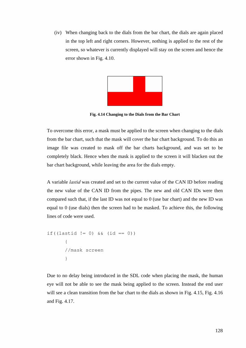
128
(iv) When changing back to the dials from the bar chart, the dials are again placed
in the top left and right corners. However, nothing is applied to the rest of the
screen, so whatever is currently displayed will stay on the screen and hence the
error shown in Fig. 4.10.
Fig. 4.14 Changing to the Dials from the Bar Chart
To overcome this error, a mask must be applied to the screen when changing to the dials
from the bar chart, such that the mask will cover the bar chart background. To do this an
image file was created to mask off the bar charts background, and was set to be
completely black. Hence when the mask is applied to the screen it will blacken out the
bar chart background, while leaving the area for the dials empty.
A variable lastid was created and set to the current value of the CAN ID before reading
the new value of the CAN ID from the pipes. The new and old CAN IDs were then
compared such that, if the last ID was not equal to 0 (use bar chart) and the new ID was
equal to 0 (use dials) then the screen had to be masked. To achieve this, the following
lines of code were used.
if((lastid != 0) && (id == 0))
{
//mask screen
}
Due to no delay being introduced in the SDL code when placing the mask, the human
eye will not be able to see the mask being applied to the screen. Instead the end user
will see a clean transition from the bar chart to the dials as shown in Fig. 4.15, Fig. 4.16
and Fig. 4.17.
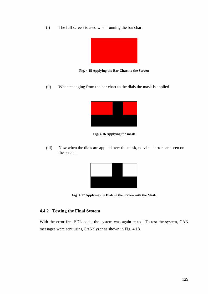
129
(i) The full screen is used when running the bar chart
Fig. 4.15 Applying the Bar Chart to the Screen
(ii) When changing from the bar chart to the dials the mask is applied
Fig. 4.16 Applying the mask
(iii) Now when the dials are applied over the mask, no visual errors are seen on the screen.
Fig. 4.17 Applying the Dials to the Screen with the Mask
4.4.2 Testing the Final System With the error free SDL code, the system was again tested. To test the system, CAN
messages were sent using CANalyzer as shown in Fig. 4.18.

130
Fig. 4.18 Messages sent using CANalyzer
These messages were then received and the desired information was placed into the
Named Pipes using the CAN program (receive_pipes). The received messages can be
seen in Fig. 4.19.
Fig. 4.19 Messages Received by the CAN program
The CAN program prints the values written into each pipe. These values are then used
to test if the data was successfully read from the pipes in the SDL program (dials_bar)
as shown in Fig. 4.20.
Fig. 4.20 SDL program Reading Data from Pipes

131
As can be seen from above, the SDL program has successfully read the data from the
pipes. The manipulated data was then displayed on the LCD screen; this data was then
used to confirm that the right values are displayed on the screen. Fig. 4.21 shows the
display for the first message as shown in Fig. 4.20.
Fig. 4.21 Output on the LCD Screen for Message 1
From Fig. 4.20, the CAN ID is equal to zero, hence the dial configuration was used, also
it can be seen that displayed speed and rpm should be 56mph and 2000rpm respectively.
Fig. 4.21 shows that all these conditions have being displayed successfully on the
screen.
The following was displayed on the screen for the second message. As shown in Fig.
4.20, it can be seen that the CAN ID is equal to 1; hence an error has occurred and the
bar chart configuration should be used. Also the speed should be 99mph and the
background used should be the tyre pressure warning (error 1). Fig. 4.22 shows that all
these conditions have been displayed successfully on the LCD screen.
Fig. 4.22 Output on the LCD Screen for Message 2

132
The following was displayed on the screen for the third message. As shown in the third
message in Fig. 4.20, it can be seen that the CAN ID is equal to 15; hence another error
has occurred so the bar chart configuration will be again used. The speed should be
145mph and the background used should be the ABS warning (error 15). Fig. 4.23
shows that all these conditions have been displayed successfully.
Fig. 4.23 Output on the LCD Screen for Message 3
After transmitting many different CAN messages from CANalyzer it was confirmed
that the final system was functioning as desired. A flow chart of the finished system is
shown in Fig. 4.24.
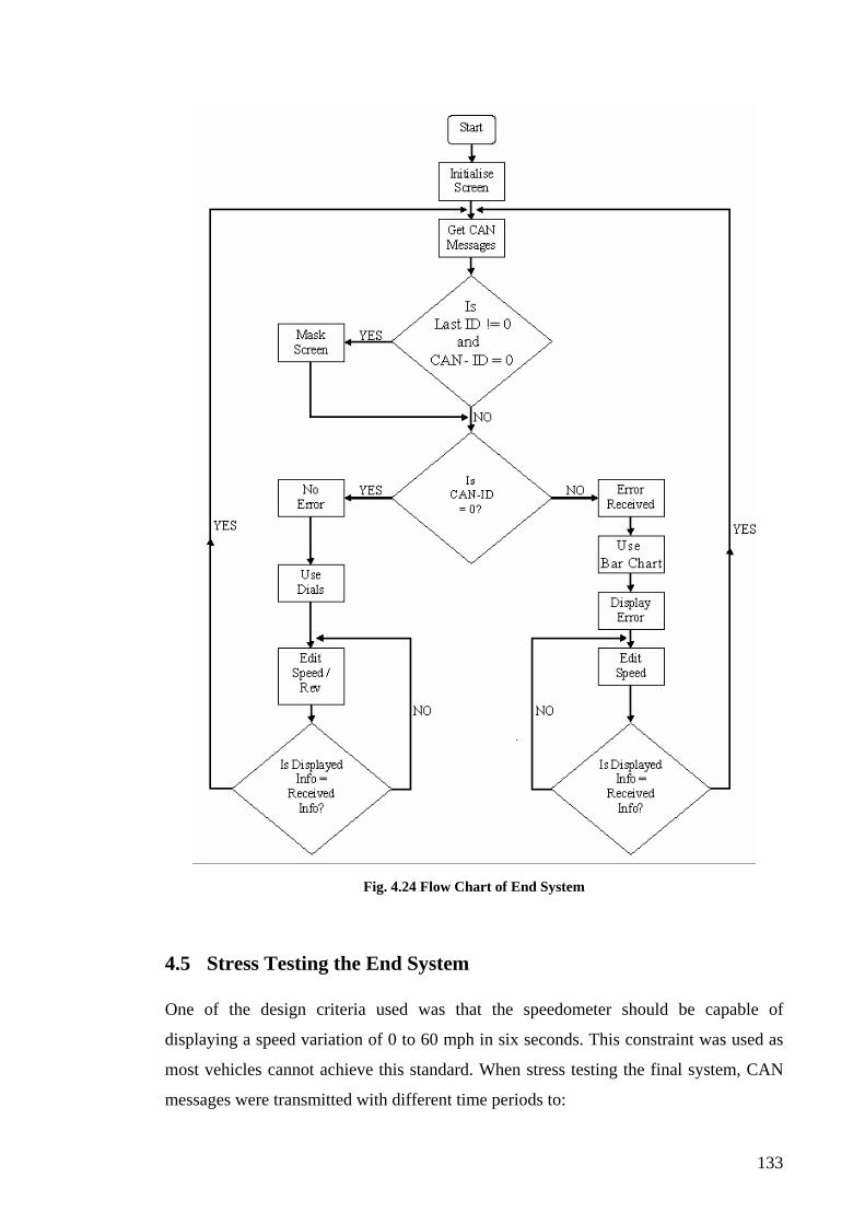
133
Fig. 4.24 Flow Chart of End System
4.5 Stress Testing the End System One of the design criteria used was that the speedometer should be capable of
displaying a speed variation of 0 to 60 mph in six seconds. This constraint was used as
most vehicles cannot achieve this standard. When stress testing the final system, CAN
messages were transmitted with different time periods to:

134
(i) Test if the system could achieve the initial goals.
(ii) Test the system for any limitations.
4.5.1 Testing System for Initial Goals As mentioned previously, the system was designed such that it could achieve the
display of 0 to 60mph in six seconds. It was decided that each CAN message would
increment the speed by 1mph, therefore to go from 0 to 60mph, 60 CAN messages
would be needed. To calculate the desired period for each CAN message to achieve 0 to
60mph in six seconds, in the following equation (4.6) was used.
100ms0.1s606
speedtimeperiod ====
(4.6)
Using the calculated period for each message, the system was then tested for successful
operation. The period of each message was set to 100ms in CANalyzer, as shown in
Fig. 4.25.
Fig. 4.25 Setting the Period of each CAN Message to 100ms in CANalyzer
With the period of each CAN message set to 100ms, with a variation of 1 mph per
message, the speed was varied from 0 to 20mph and back down again repetitively using
the CAN messages. If the system was capable of displaying these variations in speed,

135
this would hence prove that the system was capable of a 0 to 60mph change in 6
seconds. The sent messages are shown in Fig. 4.26, with a time period of 100ms.
Fig. 4.26 Messages when Stress Testing the End System
Each CAN message also increments/decrements the rpm (data byte 2) as well as the
speed (data byte 0 and 1). As the speed and rpm dials are edited using the same “do-
while” loop, hence if both were changing, the loop’s iteration time would be longer than
if only one was changing.
During this testing no errors were received on the virtual console or no glitches were
observed on the actual LCD display. Hence this proved that the final system can operate
correctly with a period of 100ms for each CAN message and therefore can display a
variation in speed of 0 to 60mph in 6 seconds.

136
4.5.2 Testing the System for Limitations As nearly all road vehicles can not achieve 0 to 60mph in 3 seconds, with the exception
of a very small number of high end sports cars, the system was then tested for correct
functionality at this data rate. The equation (4.7) was used to calculate the period of
each message for a variation of 0 to 60mph in 3 seconds.
50ms0.05s603
speedtimeperiod ====
(4.7)
The period of each message was then set to 50 ms in CANalyzer.
Fig. 4.27 Setting the Period of each CAN Message to 50ms in CANalyzer
The same message sets that had been sent previously were used again, this time with
each messages period being 50ms, as seen in Fig. 4.26. While testing the final system
using a period of 50ms and the messages shown in Fig. 4.26, with both the dials and bar
chart configurations, errors were received on the virtual console and glitches were
observed on the actual display. The error received on the virtual console is shown in
Fig. 4.28.
Fig. 4.28 Received Error using a Message Period of 50ms

137
Despite the message shown in Fig. 4.28 identifying that the error was caused by the
receiving CAN0 port’s FIFO (Named Pipe) being overrun, it was believed that this error
was due to the screen not updating at a fast enough rate. This theory was established due
to the fact that the Named Pipes used in this project were set to be blocking, i.e. a
process can not write new data into the Named Pipe until the previous data had been
read from the Named Pipe by a different process. It was believed that the display code
(dials_bar) was not capable of updating the screen and reading the new data from the
Named Pipe at a fast enough rate such that the CAN code (receive_pipes) is not waiting
to write new information into the Named Pipe. If this was the case then the CAN code
would get an overrun error as it trying to write information into the Named Pipe but it is
still blocked. To test this theory, the Named Pipes in this project were changed to be
non-blocking by editing the CAN code (receive_pipes), the CAN ID section is shown
below.
fp1 = open(SPEEDFIFO_FILE, O_WRONLY | O_NONBLOCK);
write(fp1, mes, 100);
close(fp1);
With the Named Pipes set to be non-blocking, the CAN code could overwrite the data
contained in the Named Pipe if it was not read by the display code. When the system
was re-tested using the non-block Named Pipes, the error was not received in the virtual
console, however glitches were still seen on the display. These glitches were caused by
the screen not being able to keep up with the volume of CAN messages being received.
This showed the display code was responsible for the error message received earlier.
From the stress testing it can be seen that the system is not functioning correctly when
the CAN messages were sent with a period of 50ms, hence the final system does contain
some limitations. However it is believed that these limitations could be
reduced/eradicated by tweaking the current SDL code or by enabling a different
sampling system for the CAN messages.

138
4.6 Summary This chapter reviewed the methods used and choices made when implementing the
proposed system. In this chapter the system implementation was outlined from the
design to the final system. The main points covered in this chapter were:
• The implementation of the CAN code, including the capabilities of writing to
Named Pipes which were used to pass the received data to the graphical display
process.
• The implementation of the graphical display process in SDL, this included the
capabilities of reading from Named Pipes in order to receive the data from the
CAN network.
• The testing of the final system and the eradication of any errors that may have
being present.
• The stress testing of the final system and any comments made on the outcomes
of this testing.

139
5 Conclusion

140
5.1 Introduction This chapter summarises the research and methodologies carried out for this thesis. It
outlines the results and conclusions that have been drawn from the project and offers
suggestions on how to possibly further the research.
• Chapter 2 outlined the researched literature used in the design of this project.
This chapter described the selection of a processing system, along with the OS
to run on top of the selected processor. The display technologies and IPC used in
the project were also outlined. Finally the CAN protocol was investigated.
• Chapter 3 described the configuration and design of the final system. The first
part of the chapter described the configuring of the development host, coLinux,
and the configuration and compilation of the OS and bootloader, uClinux and U-
Boot respectively. The second part of the chapter outlined the system synthesis.
This included the design of the CAN process, video processes and IPCs.
• Chapter 4 documented the implementation and testing of the final system. This
included the development of communications between the CAN network and
video processes using Named Pipes as the IPC. The testing and elimination of
any errors encountered was also outlined. Finally the system was stress tested to
observe any limitations.
5.2 Conclusions With the advances in electronics digital dashboards are now becoming available for use
in the automotive industry. The main difference between analog dashboard and digital
dashboard configurations is that the latter may easily be reconfigured. In the digital type
of configuration information can be displayed either numerically or via a digital
representation of an analog dial.
The criterion was to create a flexible digital display for use in an automotive setting
using open source hardware and software. The hardware used was an off the shelf
development board, in this case the Analog Devices Blackfin BF548. This was
combined with open source software, which included an OS, uClinux, and graphical
libraries, SDL. The system received its data from a CAN network, which was simulated
using the automotive industry standard tool “CANalyzer”.

141
To develop and compile the OS and application software, a Linux derivative, coLinux,
was used. CoLinux was selected for use in the project as it is the first Linux release to
run natively on a Windows machine. This offered many benefits, principally among
them being that only one PC was needed for all software development in Linux, while
still operating on the Windows OS. The configuration of coLinux included configuring
the network for communications between both OS and the Ethernet. The appropriate
toolchains for the compilation of uClinux, U-Boot and application code were also
installed. Lastly the “PATH” was set in coLinux to point to the proper library and linker
files when compiling any program code.
Both uClinux and U-Boot were compiled under coLinux. In the project, U-Boot was
first compiled to boot using the UART. After successfully porting this version of U-
Boot to the BF548, a second version was compiled. This version was compiled to boot
from flash memory. Using the UART U-Boot which was ported to the development
board, the flash U-Boot was saved in the BF548 flash memory. This version of U-Boot
now runs on power up. Lastly, an Ethernet connection was established in U-Boot such
that it can download the kernel on boot up. The fully configured Development Host and
Environment are shown in Fig. 5.1. For uClinux, this involved configuring a kernel to
be executable for the BF548, as well as to include all desired functionality.

142
Fig. 5.1 System Configuration Overview
Due to BF548 being the latest generation of Blackfin development boards, some of the
functionality had not been fully tested in the uClinux kernel. For example, the CAN
drivers had to be edited such that the uClinux kernel would support the CAN network.
These problems were eliminated through the combination of the review of pertinent
literature, consultation with the relevant bodies and software debugging. After
correcting the errors contained in the drivers, initial testing of the CAN network
revealed that the CAN timings were also incorrect. To correct this, new CAN variable
values were calculated, with the CAN header file been edited to include these new
calculated values. After all problems in relation to the CAN network were rectified,
application code was developed in ANSI C for the CAN process. The implemented

143
code was used to receive data from the CAN network, parse the desired information
from the received CAN data and transmit it to the SDL process.
The graphical representation of the CAN data was implemented using SDL program
code. When implementing the video process, two programmes were initially developed.
The first implemented a digital representation of a standard analog display, which
included a speedometer and a tachometer. The second implemented a digital bar chart
configuration which also displayed any error messages. After testing the two initial
programs, these were then integrated to make one video process. With the output
display configuration depending on the information received from the CAN network.
To allow communications between the CAN process and the video process, Inter
Process Communications were used, with the IPC chosen for this project being Named
Pipes. The design of the Named Pipes was achieved by writing programme code to read
and write between two processes. After fully testing this code, the same methodologies
were use to transmit information between the SDL and video processes. A basic block
diagram of the final system is shown in Fig. 5.2.
Fig. 5.2 Final System
In conclusion, it is believed that the devised system, should; (i) facilitate a significant
reduction in the design cycle time and manufacturing costs of such systems, (ii)
significantly add to the body of research and development reported to date in this field.

144
An actual implementation of this system could lead to a standardised LCD display
installed in every vehicle. Style variations between models can be easily maintained by
simply changing the images used in the video process (SDL code). Due to the open
source nature of the project, it is also believed, that its implementation would lead to
reduction in manufacturing costs and time.
5.3 Recommendations for further Research and Development While stress testing the final system, glitches were observed on the LCD screen when
transmitting CAN data with a small time period. After some investigation into the errors
it was discovered that these glitches were due to the video process not being able to
respond fast enough to the incoming data. A recommendation to improve the response
time of the video process could be to use a graphic accelerator.
A graphic accelerator can be achieved in two ways on the BF548. The first option
would be to use the open GL libraries in conjunction with the current SDL code. The
second option would be to implement DirectFB on the BF548. The video code could
then be re-written to run on DirectFB or the current SDL code can run on top of
DirectFB. Either option should improve the response time of the current SDL code.

145
References [1] V. A. W. Hillier, “Fundamentals of Automotive Electronics”, 2nd revision,
Stanley Thornes Publishing, ISBN 0748726950, 1996, pp. 323-332.
[2] William B. Ribbens, “Understanding Automotive Electronics”, 6th edition,
Elsvier Science, ISBN 0-7680-1221-X, 2003, pp. 342-347.
[3] Eric Adams, “Cars That See in the Dark”, Popular Science, Vol. 268 No. 6,
2006, pp. 24-25.
[4] The Microsoft Corporation, “Windows Automotive Data Sheet”, 2007, pp. 1-2.
[5] Jim Turley, “Embedded Systems Survey: Operating System up for Grabs”,
www.embedded.com, 2005.
[6] Cogent Computer Systems Inc., “Cogent CSB337 Hardware Reference
Manual”, 2005, pp. 4-10.
[7] Analog Devices Inc, “ADSP-BF548 Data Sheet”, 2007, pp. 1, 6-7, 13-14, 111.
[8] Analog Devices Inc, ADSP-BF548 EZ-KIT Lite Evaluation System Manual”,
2007, pp. 13-14, 49-50, 95-98.
[9] Atmel Inc, “AT91SAM9263 Data Sheet”, 2007, pp. 1, 21-27, 41-46, 48.
[10] Atmel Inc, “AT91SAM9263 Application notes”, 2007, pp. 8 -10.
[11] Atmel Inc, “AT91SAM9263 Users Guide”, 2007, pp. 5-6, 12-15.
[12] Cirrus Logic Inc, “EDB915 Data Sheet”, 2005, pp. 1, 6-8, 12.
[13] Cirrus Logic Inc, “EDB915 Product Bulletin”, 2005, pp. 1.

146
[14] H. Minorikawa, et al, “Current Status and Future Trends of Electronic
Packaging in Automotive Applications”, Society of Automotive Engineers
Technical Paper, Series 901134, 1990.
[15] C. Szydlowski, “Tradeoffs between Stand-Alone and Integrated CAN
Peripherals”, Society of Automotive Engineers Technical Paper Series 941655,
1994.
[16] Epson Inc, “Epson S1D13706 Data Sheet”, 2001, pp. 1-2.
[17] Infineon Inc, “Infineon SAK82C900 Data Sheet”, 2001, pp. 5-10.
[18] The Blackfin uClinux Project Documentation, http://docs.blackfin.uclinux.org,
2008
[19] The coLinux Project, www.colinux.org, 2007
[20] Dan Aloni, “Cooperative Linux”, Proceedings of the Linux Symposium, 2004
[21] The uClinux Project, www.uclinux.org, 2008.
[22] David McCullough, “uClinux for Linux Programmers”, The Linux Journal,
Volume 2004, Issue 123, 2004, www.linuxjournal.com.
[23] Wang Minting et al, “Research and Implementation of a uClinux-based
Embedded Browser”, IEEE Asia-Pacific Services Computing Conference, 2007.
[24] Zongqing Lu et al, “An Embedded System with uClinux based on FPGA”, IEEE
Pacific-Asia Workshop on Computational Intelligence and Industrial
Application, 2008.
[25] Gregory E. Nutt, “uClinux, File Mapping and Shared Libraries”,
www.cadenux.com, 2007.
147
[26] Curt Brune, “Introduction to Das U-Boot, the universal open source
bootloader”, Linux Devices Article, www.linuxdevices.com/articles, 2004.
[27] The “Das U-Boot” Project, “DENX U−Boot and Linux Guide”, www.denx.de,
2008
[28] Andreas Hundt, “DirectFB Overview (v0.2)”, 2004, pp. 1.
[29] Andreas Hundt, “DirectFB Overview (v0.2)”, 2004, pp. 4-5.
[30] Andreas Hundt, “DirectFB Overview (v0.2)”, 2004, pp. 5-9.
[31] Takanari Hayama et al, “DirectFB Internals – Things You Need to Know to
Write Your DirectFBgfxdriver”, Technology Consulting Company IGEL
Co.,LTD., 2008.
[32] Pablo Cesar, “What is Multimedia? Multimedia APIs”, Multimedia
Programming Lecturing Notes, Helsinki University of Technology.
[33] Denis Oliver Kropp, “Graphics Subsystem in an Embedded World – Integrating
DirectFB into a UHAPI platform”, Phillips Semiconductors Inc., 2006, pp.5.
[34] John R. Hall, “Programming Linux Games”, Loki Software Inc, 2001, pp. 69.
[35] Koray Balci, “Xface: MPEG-4 Based Open Source Toolkit for 3D Facial
Animation”, Proceedings of the Working Conference on Advanced Visual
Interfaces, 2004
[36] Pablo Cesar et al, “Open Graphical Framework for Interactive TV”, IEEE Fifth
International Symposium on Multimedia Software Engineering (ISMSE), 2003.
[37] The SDL Project, www.libsdl.com, 2008.
148
[38] Ernest Pazera et al, “Focus on SDL”, Prima Tech. Publishing, 2002, ISBN 978-
1592000302, pp.165-193.
[39] Ernest Pazera et al, “Focus on SDL”, Prima Tech. Publishing, 2002, ISBN 978-
1592000302, pp.87, 137-165.
[40] Bob Pendleton, “Why Use SDL?”, Game Programmer Article,
www.gameprogrammers.com, 2002.
[41] Pablo Cesar et al, “A Graphics Architecture for High-End Interactive Television
Terminals”, ACM Transactions on Multimedia Computing, Communications
and Applications, Vol. 2, No. 4, 2006, pp. 343 – 357.
[42] Chris Crowley, “Operating Systems: A Design-Orientated Approach”, Irwin
Books, 1997, ISBN 0-256-15151-2, pp. 231-232.
[43] Chris Crowley, “Operating Systems: A Design-Orientated Approach”, Irwin
Books, 1997, ISBN 0-256-15151-2, pp. 526-527.
[44] Chris Crowley, “Operating Systems: A Design-Orientated Approach”, Irwin
Books, 1997, ISBN 0-256-15151-2, pp. 298-305.
[45] Chris Crowley, “Operating Systems: A Design-Orientated Approach”, Irwin
Books, 1997, ISBN 0-256-15151-2, pp. 59-63.
[46] Chris Crowley, “Operating Systems: A Design-Orientated Approach”, Irwin
Books, 1997, ISBN 0-256-15151-2, pp. 308-311.
[47] Chris Crowley, “Operating Systems: A Design-Orientated Approach”, Irwin
Books, 1997, ISBN 0-256-15151-2, pp. 291-298.
[48] Daniel Pierre Bovet et al, “Understanding the Linux Kernel”, Edition: 3,
O'Reilly, 2005, ISBN 0596005652, pp. 476-498.

149
[49] Sven Goldt et al, “The Linux Programmer’s Guide”, Version 0.4, 1995, pp. 46-
47.
[50] Sven Goldt et al, “The Linux Programmer’s Guide”, Version 0.4, 1995, pp. 62.
[51] Sven Goldt et al, “The Linux Programmer’s Guide”, Version 0.4, 1995, pp. 32-
33.
[52] Sven Goldt et al, “The Linux Programmer’s Guide”, Version 0.4, 1995, pp. 27-
29.
[53] T. K. Tan et al, “Energy Macromodeling of Embedded Operating Systems”,
ACM Transactions on Embedded Computing Systems, Volume 4 , Issue 1,
2005, pp. 235.
[54] William Stallings, “Operating Systems Internal and Design Principles”, 6th
Edition, Pearson Education, 2009, ISBN: 978-0-13-603337-0, pp. 219-224.
[55] William Stallings, “Operating Systems Internal and Design Principles”, 6th
Edition, Pearson Education, 2009, ISBN: 978-0-13-603337-0, pp. 286.
[56] William Stallings, “Operating Systems Internal and Design Principles”, 6th
Edition, Pearson Education, 2009, ISBN: 978-0-13-603337-0, pp. 263-295.
[57] J.A. Williams et al, “FIFO Communication Models In Operating Systems For
Reconfigurable Computing”, Field-Programmable Custom Computing
Machines (FCCM), 2005.
[58] The Blackfin uClinux forum, http://blackfin.uclinux.org/gf/project/uclinux-
dist/forum/, 2008.
[59] Farsi, M. et al, “An overview of Controller Area Network”, Computing &
Control Engineering Journal, 1999, pp. 113-120.

150
[60] Navet, N., “Controller area network [automotive applications]”, Potentials,
IEEE, 1998, pp. 12-14.
[61] Konrad Etschberger et al, “Controller Area Network: Basics, Protocols, Chips
and Applications”, IXXAT Press, 2001, ISBN 9783000073762, pp. 43-47.
[62] Konrad Etschberger et al, “Controller Area Network: Basics, Protocols, Chips
and Applications”, IXXAT Press, 2001, ISBN 9783000073762, pp. 47-62.
[63] Siemens Microcontrollers Inc., “Controller Area Network”, 1998.
[64] Olaf Pfeiffer et al, “Embedded Networking with CAN and CANopen”, RTC
Books, 2003, ISBN 9780929392783, pp. 205-230.
[65] Bosch, “CAN Specifications Version 2”, Robert Bosch GmbH, 1991, pp. 8.
[66] Bosch, “CAN Specifications Version 2”, Robert Bosch GmbH, 1991, pp. 11-14.
[67] Bosch, “CAN Specifications Version 2”, Robert Bosch GmbH, 1991, pp. 16-18
[68] Florian Hartwich et al, “The Configuration of the CAN Bit Timing”, 6th
International CAN Conference, 1999
[69] P. Richards Microchip Inc., “Understanding Microchip’s CAN Module Bit
Timing”, 2001, pp. 1-2.
[70] P. Richards Microchip Inc., “Understanding Microchip’s CAN Module Bit
Timing”, 2001, pp. 4-8.
[71] The Source Forge Project, http://sourceforge.net/project/showfiles.php?
group_id =98788&package_id=108058, 2007
[72] M. Tim Jones, "Virtualization with coLinux”, IBM Corporation,
www.IBM.com, 2007

151
[73] Rachel Willmer, “Installing coLinux on Windows XP”,
http://www.willmer.com, 2007
[74] The Blackfin uClinux Project Toolchain Download, http://blackfin.uclinux.org
/gf/ project/toolchain/frs, 2008
[75] The Blackfin uClinux Project U-Boot Download, http://blackfin.uclinux.org/
gf/project/u-boot/frs, 2008
[76] The Blackfin uClinux Project uClinux Download, http://blackfin.uclinux.org/
gf/project/uclinux-dist/frs, 2008

152
Appendix A – Write to Pipes Program
wrpipes_test.c
// The headers 1
#include <stdio.h> 2
#include <stdlib.h> 3
#include <sys/types.h> 4
#include <sys/stat.h> 5
#include <sys/time.h> 6
#include <sys/ioctl.h> 7
#include <fcntl.h> 8
#include <unistd.h> 9
#include <string.h> 10
11
//define pipe 12
#define RFIFO_FILE "RECFIFO" 13
14
int main () 15
{ 16
int fp, i; 17
//char mes[21]; 18
19
// create pipe 20
mknod(RFIFO_FILE, S_IFIFO|0666, 0); 21
22
23
// open and write to pipe 24
char mes[] = "Hello World\n"; 25
fp = open(RFIFO_FILE, O_WRONLY); 26
write(fp, mes, 16); 27
close(fp); 28

153
29
printf("%c", mes[40]); 30
31
32
return 0; 33
34
} 35

154
Appendix B – Read from Pipes Program
rdpipes_test.c
// The headers 1
#include <stdio.h> 2
#include <stdlib.h> 3
#include <sys/types.h> 4
#include <sys/stat.h> 5
#include <sys/time.h> 6
#include <sys/ioctl.h> 7
#include <fcntl.h> 8
#include <unistd.h> 9
#include <string.h> 10
11
// define pipe 12
#define RFIFO_FILE "RECFIFO" 13
14
int main () 15
{ 16
int fp1; 17
char readbuf1[16]; 18
19
// open and read pipe 20
fp1 = open(RFIFO_FILE, O_RDONLY); 21
read(fp1, readbuf1, 16); 22
close(fp1); 23
printf("%s",readbuf1); 24
25
return 0; 26
}27

155
Appendix C – CAN Program
receive_pipes.c
//The headers 1
#include <stdio.h> 2
#include <stdlib.h> 3
#include <sys/types.h> 4
#include <sys/stat.h> 5
#include <sys/time.h> 6
#include <sys/ioctl.h> 7
#include <fcntl.h> 8
#include <unistd.h> 9
#include <string.h> 10
#include <math.h> 11
12
#include </uClinux-dist-2008R1-RC8/linux-2.6.x/drivers/char/can4linux/can4linux.h> 13
14
#define STDDEV "can0" 15
#define COMMANDNAME "receive" 16
#define VERSION "1.2" 17
18
#define RXBUFFERSIZE 100 19
20
#define SPEEDFIFO_FILE "SPEEDFIFO" 21
#define IDFIFO_FILE "IDFIFO" 22
#define REVFIFO_FILE "REVFIFO" 23
24
#ifndef TRUE 25
# define TRUE 1 26
# define FALSE 0 27
#endif 28

156
29
int sleeptime = 1000; /* standard sleep time */ 30
int debug = FALSE; 31
int baud = -1; /* dont change baud rate */ 32
int blocking = TRUE; /* open() mode */ 33
34
/* ----------------------------------------------------------------------- */ 35
36
void usage(char *s) 37
{ 38
static char *usage_text = "\ 39
Open CAN device and display read messages\n\ 40
Default device is /dev/can0. \n\ 41
Options:\n\ 42
-d - debug On\n\ 43
swich on additional debugging\n\ 44
-b baudrate (Standard uses value of /proc/sys/Can/baud)\n\ 45
-n - non-blocking mode (default blocking)\n\ 46
-s sleep sleep in ms between read() calls in non-blocking mode\n\ 47
-V version\n\ 48
\n\ 49
"; 50
fprintf(stderr, "usage: %s [options] [device]\n", s); 51
fprintf(stderr, usage_text); 52
} 53
54
55
56
/**********************************************************************57
* 58
* 59
* set_bitrate - sets the CAN bit rate 60
* 61
* 62

157
* Changing these registers only possible in Reset mode. 63
* 64
* RETURN: 65
* 66
*/ 67
68
int set_bitrate( 69
int fd, /* device descriptor */ 70
int baud /* bit rate */ 71
) 72
{ 73
Config_par_t cfg; 74
volatile Command_par_t cmd; 75
76
77
cmd.cmd = CMD_STOP; 78
ioctl(fd, CAN_IOCTL_COMMAND, &cmd); 79
80
cfg.target = CONF_TIMING; 81
cfg.val1 = baud; 82
ioctl(fd, CAN_IOCTL_CONFIG, &cfg); 83
84
cmd.cmd = CMD_START; 85
ioctl(fd, CAN_IOCTL_COMMAND, &cmd); 86
return 0; 87
} 88
89
90
/**********************************************************************91
* 92
* 93
* main - 94
* 95
* 96

158
*/ 97
98
int main(int argc,char **argv) 99
{ 100
int fd; 101
int got; 102
int c; 103
char *pname; 104
extern char *optarg; 105
extern int optind; 106
107
canmsg_t rx[RXBUFFERSIZE]; 108
char device[50]; 109
int messages_to_read = 1; 110
111
pname = *argv; 112
113
/* parse command line */ 114
while ((c = getopt(argc, argv, "b:dhs:nV")) != EOF) { 115
switch (c) { 116
case 'b': 117
baud = atoi(optarg); 118
break; 119
case 's': 120
sleeptime = atoi(optarg); 121
break; 122
case 'd': 123
debug = TRUE; 124
break; 125
case 'n': 126
blocking = FALSE; 127
messages_to_read = RXBUFFERSIZE; 128
break; 129
case 'V': 130

159
printf("%s %s\n", argv[0], " V " VERSION ", " __DATE__ ); 131
exit(0); 132
break; 133
134
/* not used, devicename is parameter */ 135
case 'D': 136
if ( 137
/* path ist starting with '.' or '/', use it as it is */ 138
optarg[0] == '.' 139
|| 140
optarg[0] == '/' 141
) { 142
sprintf(device, "%s", optarg); 143
144
} else { 145
sprintf(device, "/dev/%s", optarg); 146
} 147
break; 148
case 'h': 149
default: usage(pname); exit(0); 150
} 151
} 152
153
/* look for additional arguments given on the command line */ 154
if ( argc - optind > 0 ) { 155
/* at least one additional argument, the device name is given */ 156
char *darg = argv[optind]; 157
158
if ( 159
/* path ist starting with '.' or '/', use it as it is */ 160
darg[0] == '.' 161
|| 162
darg[0] == '/' 163
) { 164

160
sprintf(device, "%s", darg); 165
} else { 166
sprintf(device, "/dev/%s", darg); 167
} 168
} else { 169
sprintf(device, "/dev/%s", STDDEV); 170
} 171
172
if ( debug == TRUE ) { 173
printf("%s %s\n", argv[0], " V " VERSION ", " __DATE__ ); 174
printf("(c) 1996-2006 port GmbH\n"); 175
printf(" using canmsg_t with %d bytes\n", sizeof(canmsg_t)); 176
printf(" CAN device %s opened in %sblocking mode\n", 177
device, blocking ? "" : "non-"); 178
179
} 180
181
sleeptime *= 1000; 182
183
if(blocking == TRUE) { 184
/* fd = open(device, O_RDWR); */ 185
fd = open(device, O_RDONLY); 186
} else { 187
fd = open(device, O_RDONLY | O_NONBLOCK); 188
} 189
if( fd < 0 ) { 190
fprintf(stderr,"Error opening CAN device %s\n", device); 191
perror("open"); 192
exit(1); 193
} 194
if (baud > 0) { 195
if ( debug == TRUE ) { 196
printf("change Bit-Rate to %d Kbit/s\n", baud); 197
} 198

161
set_bitrate(fd, baud); 199
} 200
201
/* printf("waiting for msg at %s\n", device); */ 202
203
////////////// Start Of Edit ///////////////// 204
while(1) { 205
got=read(fd, &rx, messages_to_read); 206
int fp1, fp2, fp3; 207
umask(0); 208
mknod(SPEEDFIFO_FILE, S_IFIFO|0666, 0); 209
mknod(IDFIFO_FILE, S_IFIFO|0666, 0); 210
mknod(REVFIFO_FILE, S_IFIFO|0666, 0); 211
char x[10]; 212
char w[10]; 213
char id[10]; 214
char mes[10]; 215
char y[10]; 216
char rev[10]; 217
int byte1, byte2, speed, byte3; 218
219
if( got > 0) { 220
int i; 221
int j; 222
223
for(i = 0; i < got; i++) { 224
printf("Received with ret=%d: %12lu.%06lu id=%ld\n", 225
got, 226
rx[i].timestamp.tv_sec, 227
rx[i].timestamp.tv_usec, 228
rx[i].id); 229
230
sprintf(w, "%d", rx[i].id); 231
strcpy(id, w); 232

162
233
234
printf("\tlen=%d msg=", rx[i].length); 235
for(j = 0; j < rx[i].length; j++) { 236
printf(" %02x", rx[i].data[j]); 237
} 238
239
byte1 = ("%d", rx[i].data[0]); 240
byte2 = ("%d", rx[i].data[1]); 241
byte3 = ("%d", rx[i].data[2]); 242
243
speed = byte1*pow(16,2) + byte2; 244
245
sprintf(x, "%d", speed); 246
strcpy(mes, x); 247
248
sprintf(y, "%d", byte3); 249
strcpy(rev, y); 250
251
printf(" flags=0x%02x\n", rx[i].flags ); 252
fflush(stdout); 253
} 254
} else { 255
printf("Received with ret=%d\n", got); 256
fflush(stdout); 257
} 258
if(blocking == FALSE) { 259
/* wait some time before doing the next read() */ 260
usleep(sleeptime); 261
} 262
263
fp1 = open(SPEEDFIFO_FILE, O_WRONLY); 264
write(fp1, mes, 100); 265
close(fp1); 266

163
printf("mes = %s\n", mes); 267
268
fp2 = open(IDFIFO_FILE, O_WRONLY); 269
write(fp2, id, 100); 270
close(fp2); 271
printf("id = %s\n", id); 272
273
fp3 = open(REVFIFO_FILE, O_WRONLY); 274
write(fp3, rev, 100); 275
close(fp3); 276
printf("rev = %s\n", rev); 277
278
} 279
////////// End Of Edit //////////////// 280
281
close(fd); 282
return 0; 283
}284

164
Appendix D – Video Program
dials_bar.c
//The headers 1
#include "SDL.h" 2
#include "SDL_image.h" 3
#include "stdlib.h" 4
#include "stdbool.h" 5
#include <stdio.h> 6
#include <stdlib.h> 7
#include <sys/types.h> 8
#include <sys/stat.h> 9
#include <sys/time.h> 10
#include <sys/ioctl.h> 11
#include <fcntl.h> 12
#include <unistd.h> 13
#include <string.h> 14
#include <math.h> 15
16
#define SPEEDFIFO_FILE "SPEEDFIFO" 17
#define IDFIFO_FILE "IDFIFO" 18
#define REVFIFO_FILE "REVFIFO" 19
20
char readbuf1[10]; 21
char readbuf2[10]; 22
char readbuf3[10]; 23
24
//The attributes of the screen 25
const int SCREEN_WIDTH = 480; 26
const int SCREEN_HEIGHT = 272; 27
const int SCREEN_BPP = 16; 28

165
29
//The surfaces that will be used 30
SDL_Surface *message1 = NULL; 31
SDL_Surface *message2 = NULL; 32
SDL_Surface *message3 = NULL; 33
SDL_Surface *background = NULL; 34
SDL_Surface *mask = NULL; 35
SDL_Surface *screen = NULL; 36
37
bool quit = false; 38
int fp1,fp2,id,fp3,z,t,m,j,i,k,s,lastid; 39
int del = 5; 40
int rpm_value; 41
int last_rpm = 0; 42
int mph_value; 43
int last_mph = 0; 44
int rpm_finished = 0; 45
int mph_finished = 0; 46
char rpm[25]; 47
char mph[25]; 48
char c[25]; 49
char d[25]; 50
char bground[50]; 51
char mk[25]= "images/mph/mask.PNG"; 52
53
54
55
//The event structure 56
SDL_Event event; 57
58
void apply_surface( int x, int y, SDL_Surface* source, SDL_Surface* destination ) 59
{ 60
//Make a temporary rectangle to hold the offsets 61
SDL_Rect offset; 62

166
63
//Give the offsets to the rectangle 64
offset.x = x; 65
offset.y = y; 66
67
//Blit the surface 68
SDL_BlitSurface( source, NULL, destination, &offset ); 69
} 70
71
bool init() 72
{ 73
//Initialize all SDL subsystems 74
if( SDL_Init( SDL_INIT_EVERYTHING ) == -1 ) 75
{ 76
return false; 77
} 78
79
//Set up the screen 80
screen = SDL_SetVideoMode( SCREEN_WIDTH, SCREEN_HEIGHT, 81
SCREEN_BPP, SDL_SWSURFACE ); 82
83
//If there was an error in setting up the screen 84
if( screen == NULL ) 85
{ 86
return false; 87
} 88
89
//If everything initialized fine 90
return true; 91
} 92
93
void quit_prog() 94
{ 95
// SDL_FreeSurface( message1 ); 96

167
//Quit SDL 97
SDL_Quit(); 98
exit(0); 99
} 100
101
void mask_screen() 102
{ 103
mask = IMG_Load( mk ); 104
apply_surface( 0, 0, mask, screen ); 105
SDL_FreeSurface( mask ); 106
} 107
108
int get_can(t, mph_value, id, lastid, rpm_value) 109
int *t, *mph_value, *id, *rpm_value, *lastid; 110
{ 111
//////////// Speed Pipe ///////////// 112
fp1 = open(SPEEDFIFO_FILE, O_RDONLY); 113
read(fp1, readbuf1, 10); 114
close(fp1); 115
116
z = atoi(readbuf1); 117
*mph_value = ceil(z/18); 118
printf("mph_value = %d\n",*mph_value); 119
if (*mph_value > 145) 120
{ 121
*mph_value = 145; 122
} 123
124
*t = ceil(z/30); 125
if (*t > 87) 126
{ 127
*t = 87; 128
} 129
130

168
////////// ID Pipe ///////////////// 131
fp2 = open(IDFIFO_FILE, O_RDONLY); 132
read(fp2, readbuf2, 10); 133
close(fp2); 134
*lastid = *id; 135
*id = atoi(readbuf2); 136
printf("id = %d\n",*id); 137
sprintf(bground, "images/bar/err%d.PNG", *id); 138
139
140
141
///////////// RPM Pipe /////////////////// 142
fp3 = open(REVFIFO_FILE, O_RDONLY); 143
read(fp3, readbuf3, 10); 144
close(fp3); 145
*rpm_value = atoi(readbuf3); 146
147
if (*rpm_value > 300) 148
{ 149
*rpm_value = 300; 150
} 151
*rpm_value = *rpm_value * 20; 152
printf("rpm_value = %d\n\n",*rpm_value); 153
} 154
155
156
int dials(rpm_value, last_rpm , mph_value, last_mph, rpm_finished, mph_finished) 157
int *rpm_value, *last_rpm, *mph_value, *last_mph, *rpm_finished, *mph_finished; 158
{ 159
do{ 160
if(*rpm_finished != 1) 161
{ 162
if(*rpm_value > *last_rpm) 163
{ 164

169
*last_rpm = *last_rpm + 20; 165
} 166
else if(*rpm_value < *last_rpm) 167
{ 168
*last_rpm = *last_rpm - 20; 169
} 170
sprintf(rpm, "images/rpm/%d.png", *last_rpm); 171
172
message2 = IMG_Load( rpm ); 173
apply_surface( 280, 0, message2, screen ); 174
if( SDL_Flip( screen ) == -1 ) 175
{ 176
return 1; 177
} 178
SDL_FreeSurface( message2 ); 179
180
if(*last_rpm == *rpm_value) 181
{ 182
*rpm_finished = 1; 183
} 184
} 185
if(*mph_finished != 1) 186
{ 187
if(*mph_value < *last_mph) 188
{ 189
*last_mph = *last_mph - 1; 190
} 191
else if (*mph_value > *last_mph) 192
{ 193
*last_mph = *last_mph + 1; 194
} 195
sprintf(mph, "images/mph/%d.png", *last_mph); 196
197
message1 = IMG_Load( mph ); 198

170
apply_surface( 0, 0, message1, screen ); 199
if( SDL_Flip( screen ) == -1 ) 200
{ 201
return 1; 202
} 203
SDL_FreeSurface( message1 ); 204
205
if(*last_mph == *mph_value) 206
{ 207
*mph_finished = 1; 208
} 209
} 210
} 211
while((*rpm_finished != 1) || (*mph_finished != 1)); 212
} 213
214
int green_up(i,t) 215
int *i,*t; 216
{ 217
s = *i; 218
if (s <= *t) 219
{ 220
for (s=*i;((s<42)&&(s<*t));s++) 221
{ 222
background = IMG_Load( bground ); 223
message1 = IMG_Load( "images/bar/green.PNG" ); 224
apply_surface( 0, 0, background, screen ); 225
for (k=0;k<=s;k++) 226
{ 227
apply_surface( j, 212, message1, screen ); 228
j=j+4; 229
} 230
if( SDL_Flip( screen ) == -1 ) 231
{ 232

171
return 1; 233
} 234
SDL_Delay( del ); 235
SDL_FreeSurface( message1 ); 236
SDL_FreeSurface( background ); 237
j = 56; 238
} 239
*i=s; 240
} 241
} 242
243
int yellow_up(i,t) 244
int *i,*t; 245
{ 246
s = *i; 247
if (s <= *t) 248
{ 249
for (s=*i;((s<60)&&(s<*t));s++) 250
{ 251
background = IMG_Load( bground ); 252
message2 = IMG_Load( "images/bar/yellow.PNG" ); 253
apply_surface( 0, 0, background, screen ); 254
for (k=0;k<=s;k++) 255
{ 256
apply_surface( j, 212, message2, screen ); 257
j=j+4; 258
259
} 260
if( SDL_Flip( screen ) == -1 ) 261
{ 262
return 1; 263
} 264
SDL_Delay( del ); 265
SDL_FreeSurface( message2 ); 266

172
SDL_FreeSurface( background ); 267
j = 56; 268
} 269
*i=s; 270
} 271
} 272
273
274
int red_up(i,t) 275
int *i,*t; 276
{ 277
s = *i; 278
if (s <= *t) 279
{ 280
for (s=*i;((s<88)&&(s<*t));s++) 281
{ 282
background = IMG_Load( bground ); 283
message3 = IMG_Load( "images/bar/red.PNG" ); 284
apply_surface( 0, 0, background, screen ); 285
for (k=0;k<=s;k++) 286
{ 287
apply_surface( j, 212, message3, screen ); 288
j=j+4; 289
290
} 291
if( SDL_Flip( screen ) == -1 ) 292
{ 293
return 1; 294
} 295
SDL_Delay( del ); 296
SDL_FreeSurface( message3 ); 297
SDL_FreeSurface( background ); 298
j = 56; 299
} 300

173
*i=s; 301
} 302
} 303
304
int red_down(i,t) 305
int *i, *t; 306
{ 307
s = *i; 308
if (s >= *t) 309
{ 310
for (s=*i;((s>=60)&&(s>*t));s--) 311
{ 312
background = IMG_Load( bground ); 313
message3 = IMG_Load( "images/bar/red.PNG" ); 314
apply_surface( 0, 0, background, screen ); 315
for (m=1;m<s;m++) 316
{ 317
apply_surface( j, 212, message3, screen ); 318
j=j+4; 319
320
} 321
if( SDL_Flip( screen ) == -1 ) 322
{ 323
return 1; 324
} 325
SDL_Delay( del ); 326
SDL_FreeSurface( message3 ); 327
SDL_FreeSurface( background ); 328
j = 56; 329
} 330
*i=s; 331
} 332
333
} 334
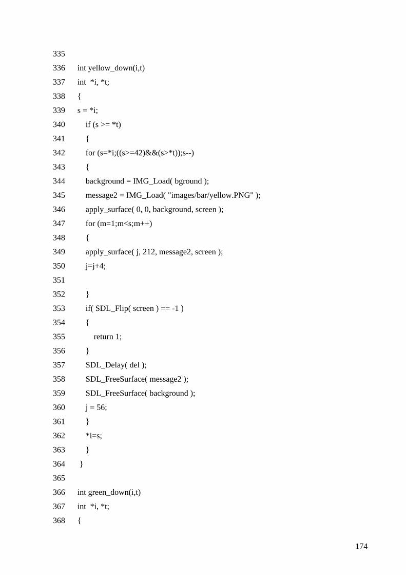
174
335
int yellow_down(i,t) 336
int *i, *t; 337
{ 338
s = *i; 339
if (s >= *t) 340
{ 341
for (s=*i;((s>=42)&&(s>*t));s--) 342
{ 343
background = IMG_Load( bground ); 344
message2 = IMG_Load( "images/bar/yellow.PNG" ); 345
apply_surface( 0, 0, background, screen ); 346
for (m=1;m<s;m++) 347
{ 348
apply_surface( j, 212, message2, screen ); 349
j=j+4; 350
351
} 352
if( SDL_Flip( screen ) == -1 ) 353
{ 354
return 1; 355
} 356
SDL_Delay( del ); 357
SDL_FreeSurface( message2 ); 358
SDL_FreeSurface( background ); 359
j = 56; 360
} 361
*i=s; 362
} 363
} 364
365
int green_down(i,t) 366
int *i, *t; 367
{ 368
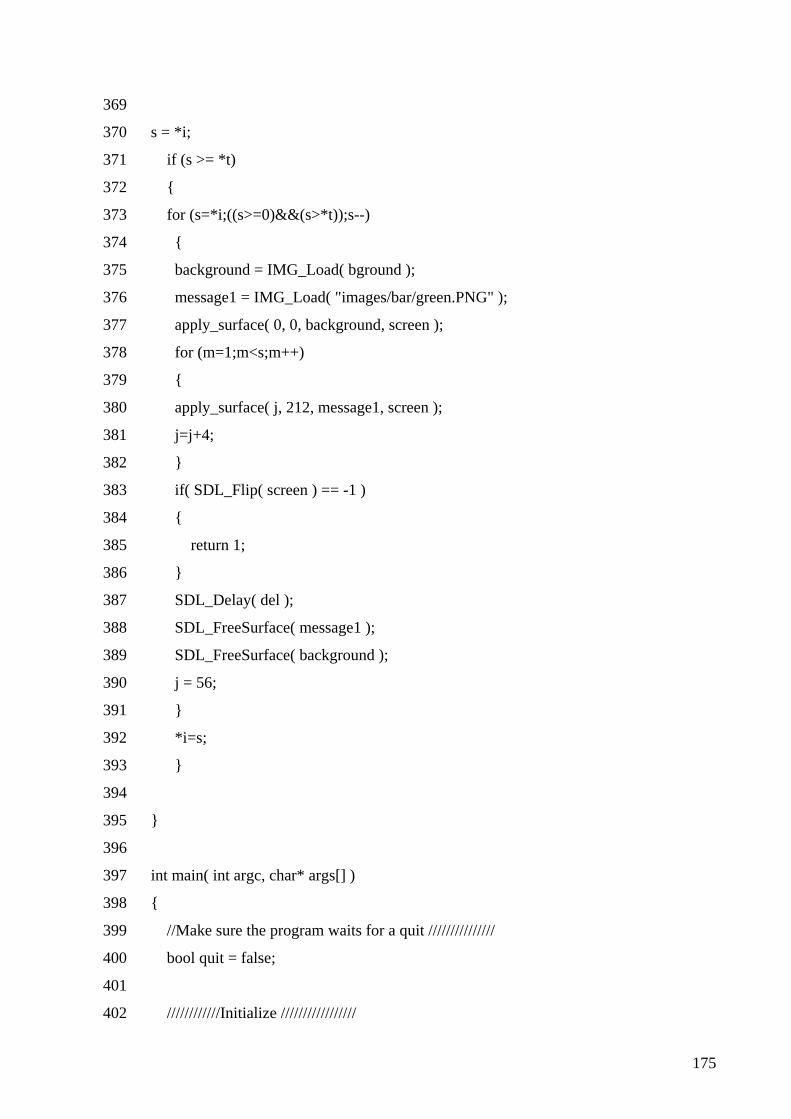
175
369
s = *i; 370
if (s >= *t) 371
{ 372
for (s=*i;((s>=0)&&(s>*t));s--) 373
{ 374
background = IMG_Load( bground ); 375
message1 = IMG_Load( "images/bar/green.PNG" ); 376
apply_surface( 0, 0, background, screen ); 377
for (m=1;m<s;m++) 378
{ 379
apply_surface( j, 212, message1, screen ); 380
j=j+4; 381
} 382
if( SDL_Flip( screen ) == -1 ) 383
{ 384
return 1; 385
} 386
SDL_Delay( del ); 387
SDL_FreeSurface( message1 ); 388
SDL_FreeSurface( background ); 389
j = 56; 390
} 391
*i=s; 392
} 393
394
} 395
396
int main( int argc, char* args[] ) 397
{ 398
//Make sure the program waits for a quit /////////////// 399
bool quit = false; 400
401
////////////Initialize ///////////////// 402

176
if( init() == false ) 403
{ 404
return 1; 405
} 406
407
while( quit == false ) 408
{ 409
410
/////mask screen when going from bar graph to dials////////// 411
if((lastid != 0) && (id == 0)) 412
{ 413
mask_screen(); 414
} 415
416
///// id = 0; no errors; use dials /////////////////////// 417
if(id == 0) 418
{ 419
dials(&rpm_value, &last_rpm ,&mph_value, &last_mph, &rpm_finished, 420
&mph_finished); 421
422
rpm_finished = 0; 423
mph_finished = 0; 424
i = ((last_mph*18)/30); 425
} 426
427
///// id != 0; errors; use bar graph and dispaly error /////////////////////// 428
else if (id != 0) 429
{ 430
do{ 431
j=56; 432
if ((i>=0) && (i<42) && (t>i)) 433
{ 434
green_up(&i, &t); 435
} 436

177
else if ((i>=0) && (i<42) && (t<i)) 437
{ 438
green_down(&i, &t); 439
} 440
else if ((i>=42) && (i<60) && (t>i)) 441
{ 442
yellow_up(&i, &t); 443
} 444
else if ((i>=42) && (i<60) && (t<i)) 445
{ 446
yellow_down(&i, &t); 447
} 448
else if ((i>=60) && (i<88) && (t>i)) 449
{ 450
red_up(&i, &t); 451
} 452
else if ((i>=60) && (i<88) && (t<i)) 453
{ 454
red_down(&i, &t); 455
} 456
} 457
while (t != i); 458
last_mph = ((i*30)/18); 459
last_rpm = rpm_value; 460
} 461
462
/////////// Get Info from CAN ////////////////// 463
get_can(&t,&mph_value, &id, &lastid, &rpm_value); 464
465
while( SDL_PollEvent( &event ) ) 466
{ 467
//If the user has Xed out the window 468
if( event.type == SDL_QUIT ) 469
{ 470

178
//Quit the program 471
quit_prog(); 472
} 473
} 474
} 475
476
477
return 0; 478