Fitting Models to Data

1

BMVC 2015 Tutorial

Andrew Fitzgibbon, Microsoft

PEOPLE

Finding Nemo: Deformable Object Class Modelling using Curve Matching CVPR ’10Mukta Prasad, Andrew Fitzgibbon, Andrew Zisserman, Luc Van Gool

KinÊtre: Animating the World with the Human Body UIST ’12Jiawen Chen, Shahram Izadi, Andrew Fitzgibbon

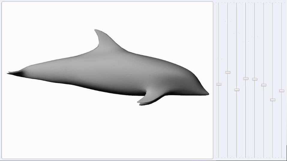
What shape are dolphins? Building 3D morphable models from 2D images PAMI ’13Tom Cashman, Andrew Fitzgibbon

User-Specific Hand Modeling from Monocular Depth Sequences CVPR ’14Jonathan Taylor, Richard Stebbing, Varun Ramakrishna, Cem Keskin, Jamie Shotton, Shahram Izadi, Andrew Fitzgibbon, Aaron Hertzmann

Real-Time Non-Rigid Reconstruction Using an RGB-D Camera SIGGRAPH ’14Michael Zollhöfer, Matthias Nießner, Shahram Izadi, Christoph Rhemann, Christopher Zach, Matthew Fisher, Chenglei Wu, Andrew Fitzgibbon, Charles Loop, Christian Theobalt, Marc Stamminger

Learning an Efficient Model of Hand Shape Variation from Depth Images CVPR ’15Sameh Khamis, Jonathan Taylor, Jamie Shotton, Cem Keskin, Shahram Izadi, Andrew Fitzgibbon

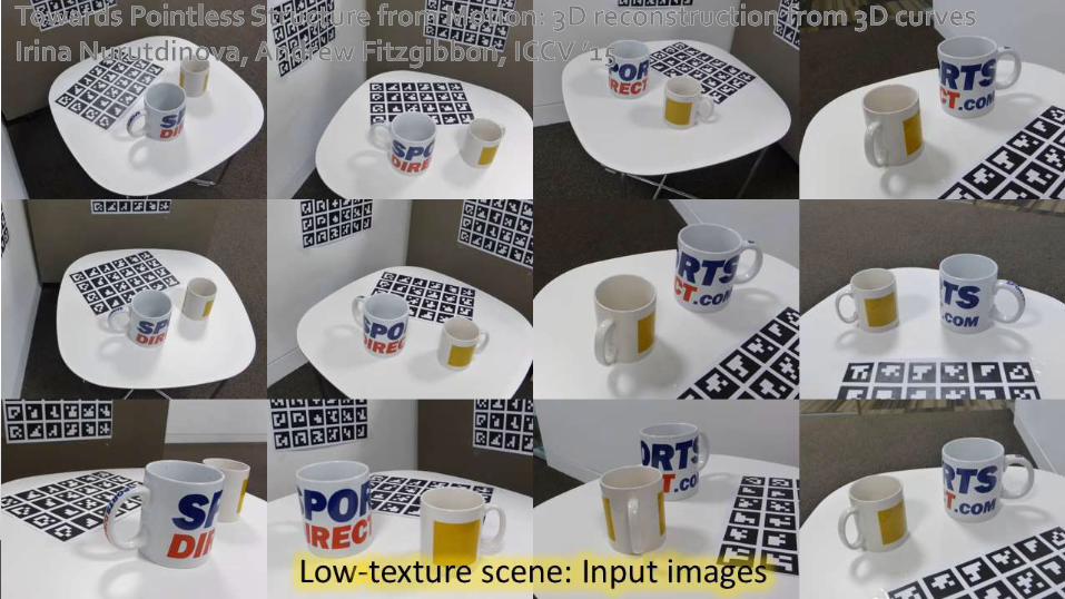
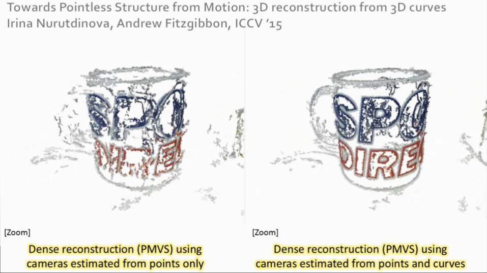
Towards Pointless Structure from Motion: 3D reconstruction from 3D curves ICCV ’15Irina Nurutdinova, Andrew Fitzgibbon

Secrets of Matrix Factorization: Approximations, Numerics and Manifold Optimization ICCV ’15Je Hyeong Hong, Andrew Fitzgibbon

LEARN HOW TO SOLVE HARD VISION PROBLEMS, USING TOOLS THAT MAY APPEAR INELEGANT, BUT ARE MUCH SMARTER THAN THEY LOOK.

Goal

3

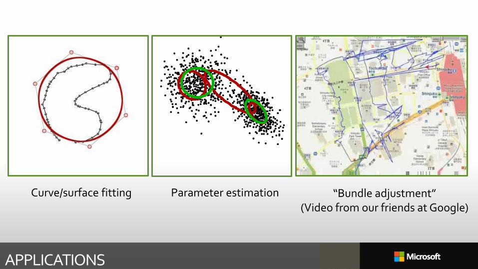
APPLICATIONS

Curve/surface fitting Parameter estimation “Bundle adjustment”(Video from our friends at Google)

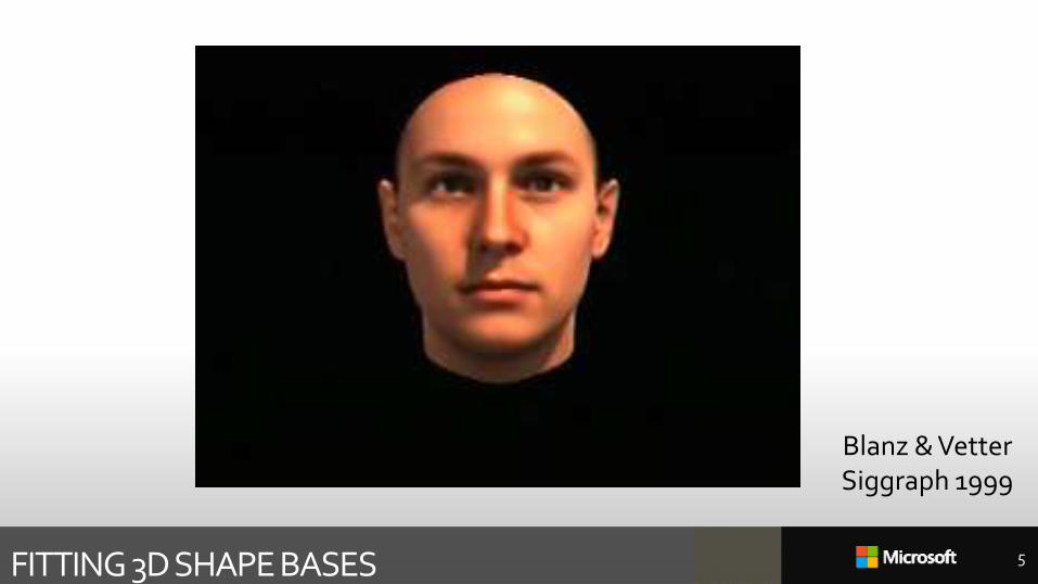
FITTING 3D SHAPE BASES 5

Blanz & VetterSiggraph 1999

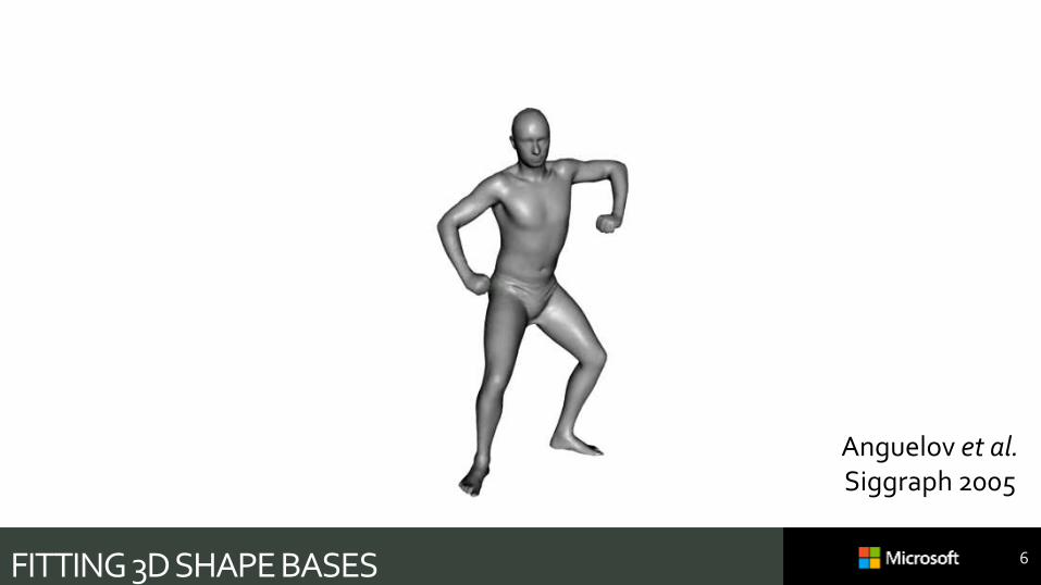
FITTING 3D SHAPE BASES 6

Anguelov et al.Siggraph 2005

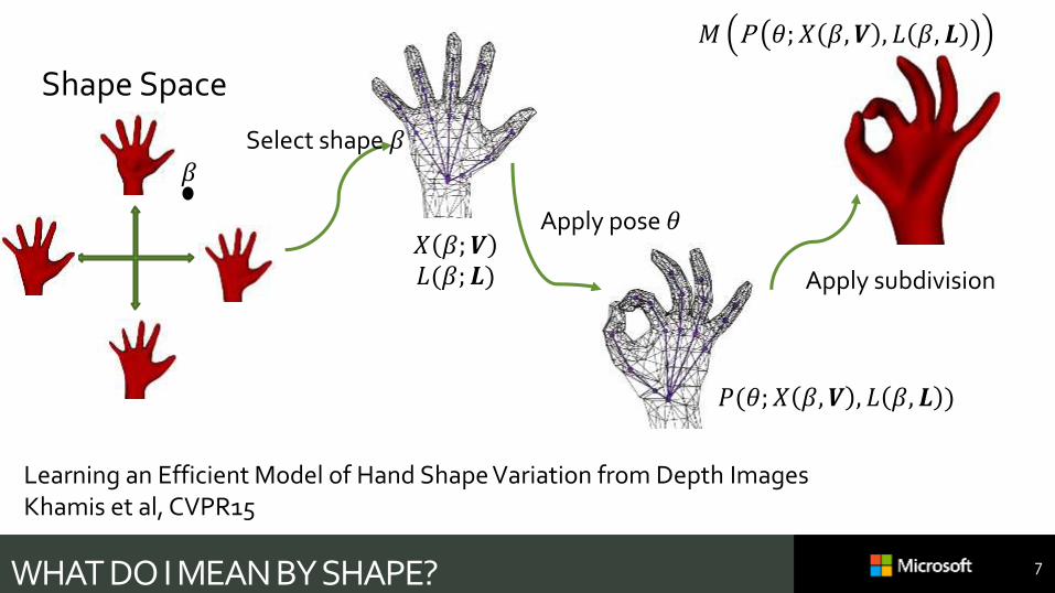
WHAT DO I MEAN BY SHAPE? 7

Learning an Efficient Model of Hand Shape Variation from Depth ImagesKhamis et al, CVPR15

𝑋 𝛽; 𝑽𝐿(𝛽; 𝑳)

Shape Space

𝑃(𝜃; 𝑋 𝛽, 𝑽 , 𝐿 𝛽, 𝑳 )

𝑀 P 𝜃; 𝑋 𝛽, 𝑽 , 𝐿 𝛽, 𝑳

𝛽Select shape 𝛽

Apply pose 𝜃

Apply subdivision

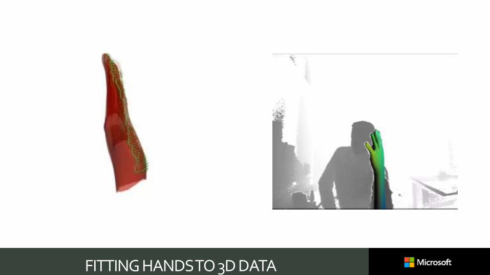
FITTING HANDS TO 3D DATA

9

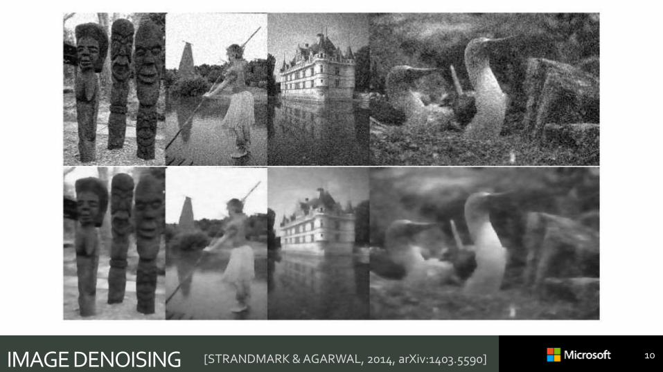
IMAGE DENOISING 10[STRANDMARK & AGARWAL, 2014, arXiv:1403.5590]

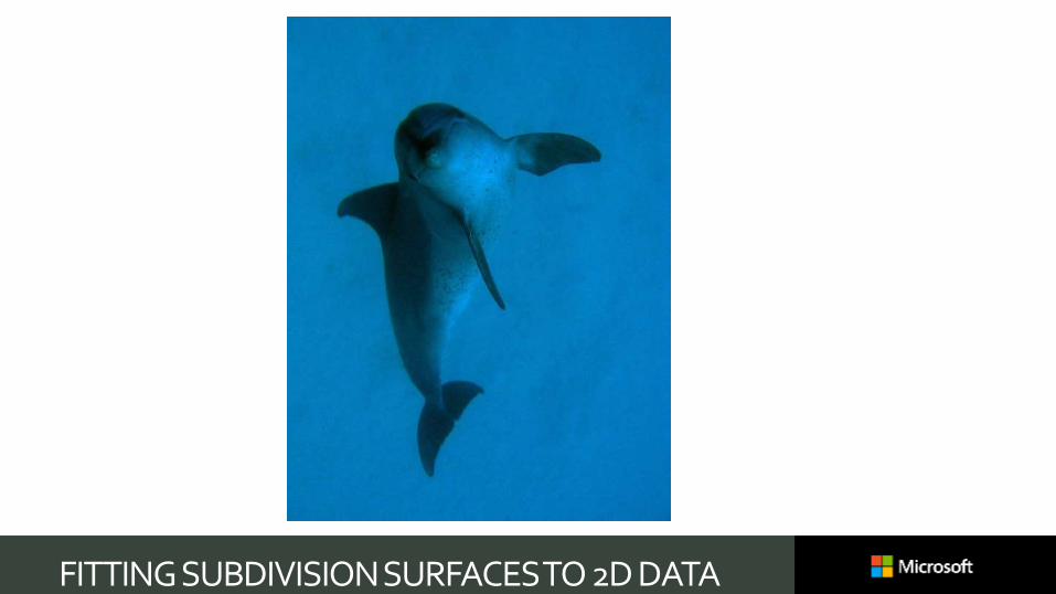
FITTING SUBDIVISION SURFACES TO 2D DATA

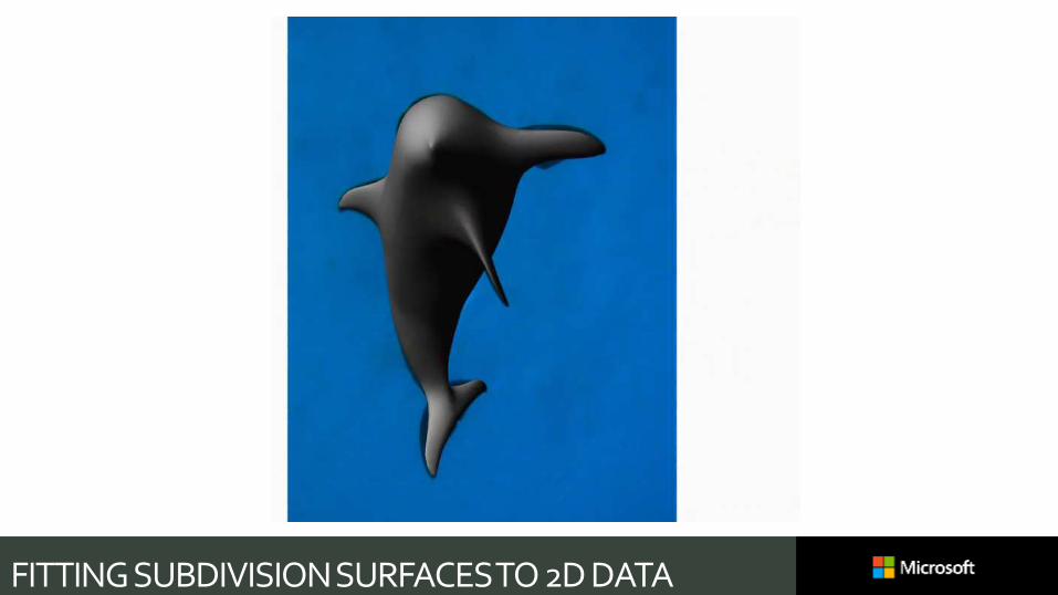
FITTING SUBDIVISION SURFACES TO 2D DATA

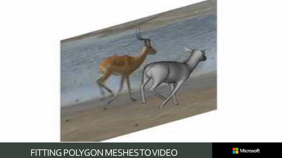
FITTING POLYGON MESHES TO VIDEO

14

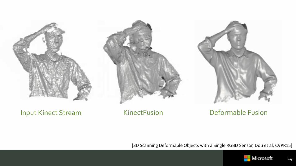
[3D Scanning Deformable Objects with a Single RGBD Sensor, Dou et al, CVPR15]

Input Kinect Stream KinectFusion Deformable Fusion

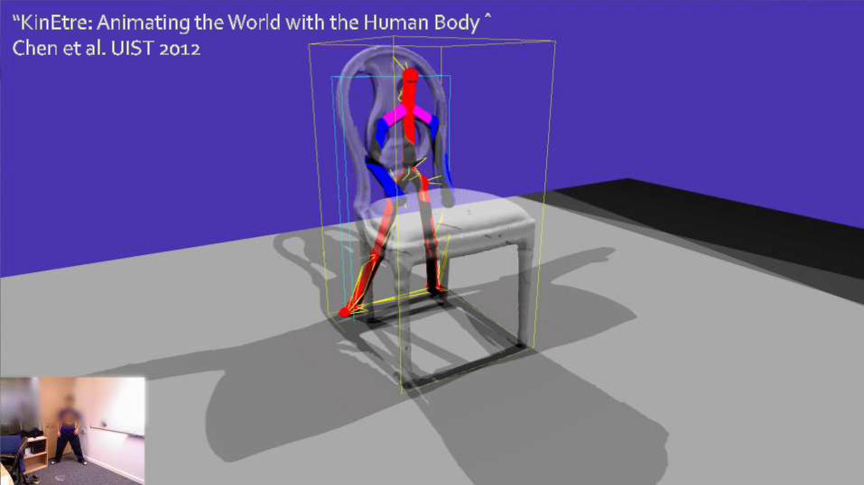
KINÊTRE 15

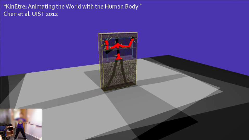
KINÊTRE 16

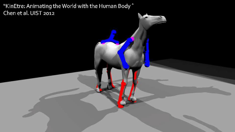
KINÊTRE 17

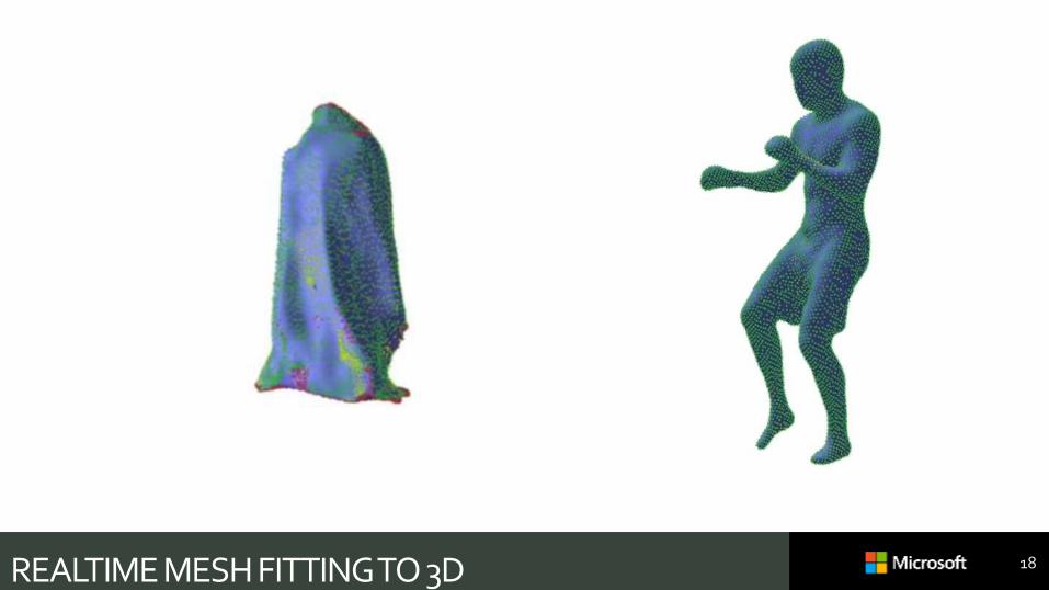
REALTIME MESH FITTING TO 3D 18

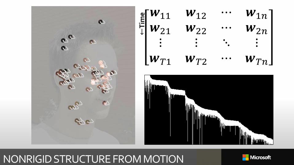
NONRIGID STRUCTURE FROM MOTION

𝒘11 𝒘12 ⋯ 𝒘1𝑛

𝒘21 𝒘22 ⋯ 𝒘2𝑛

⋮ ⋮ ⋱ ⋮𝒘𝑇1 𝒘𝑇2 ⋯ 𝒘𝑇𝑛

←T

ime

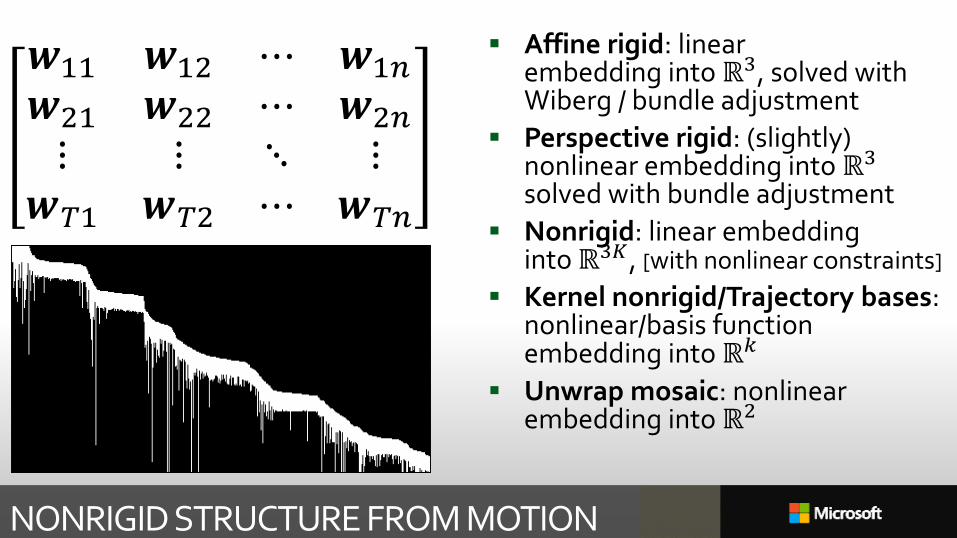
NONRIGID STRUCTURE FROM MOTION

Affine rigid: linear embedding into ℝ3, solved with Wiberg / bundle adjustment

Perspective rigid: (slightly) nonlinear embedding into ℝ3

solved with bundle adjustment

Nonrigid: linear embedding into ℝ3𝐾, [with nonlinear constraints]

Kernel nonrigid/Trajectory bases: nonlinear/basis function embedding into ℝ𝑘

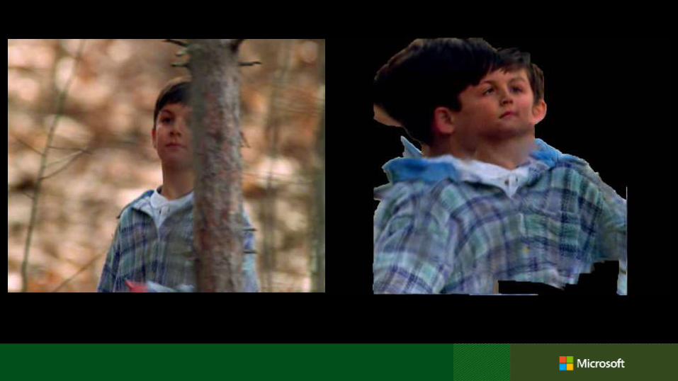
Unwrap mosaic: nonlinear embedding into ℝ2

𝒘11 𝒘12 ⋯ 𝒘1𝑛

𝒘21 𝒘22 ⋯ 𝒘2𝑛

⋮ ⋮ ⋱ ⋮𝒘𝑇1 𝒘𝑇2 ⋯ 𝒘𝑇𝑛

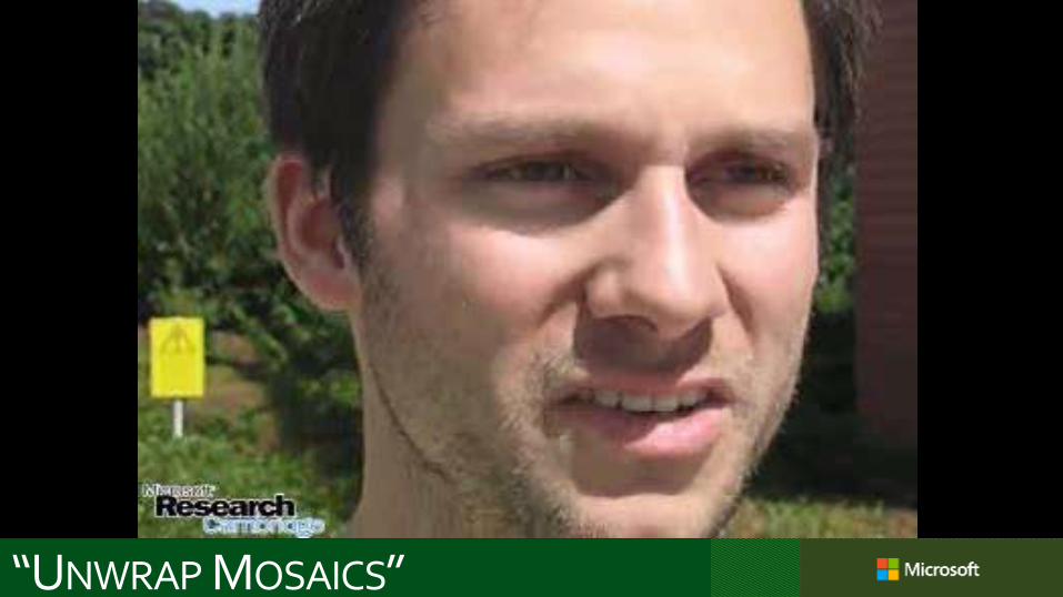
“UNWRAP MOSAICS”

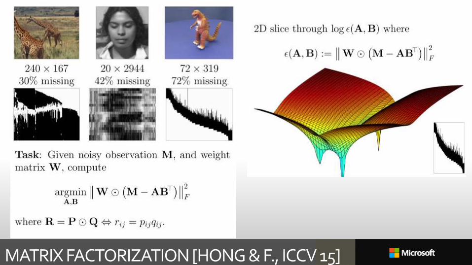
MATRIX FACTORIZATION [HONG & F., ICCV 15]

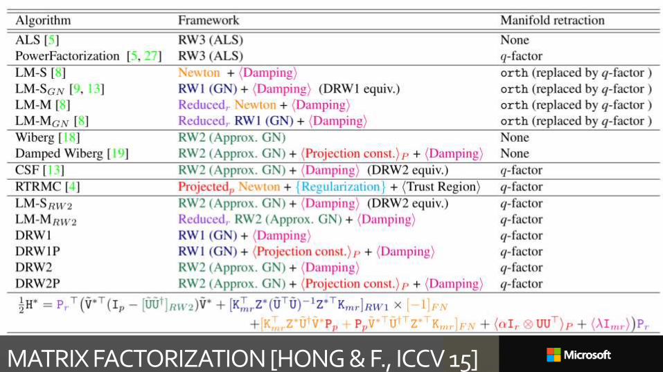
MATRIX FACTORIZATION [HONG & F., ICCV 15]

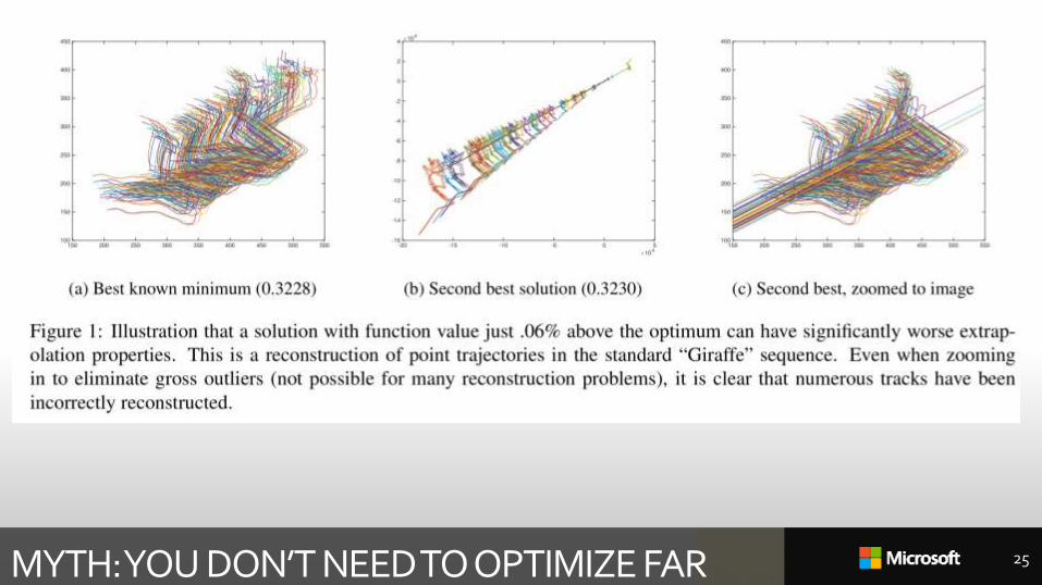
MYTH: YOU DON’T NEED TO OPTIMIZE FAR 25

BUT POINTS ARE TOO EASY…

clownfish

OBJECT CATEGORY MODELS

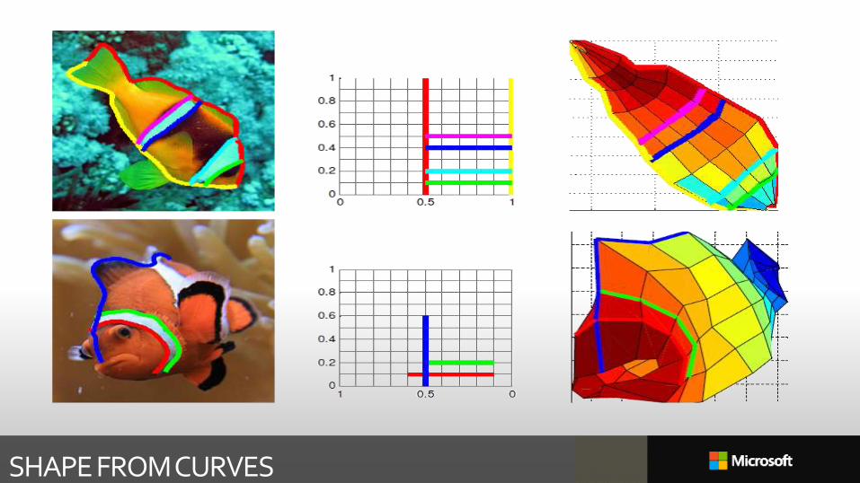
SHAPE FROM CURVES

34

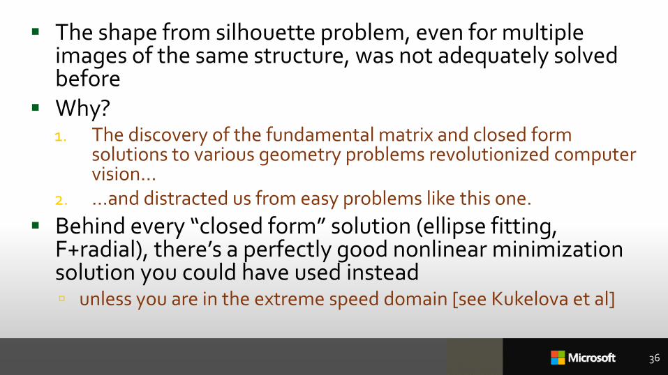
The shape from silhouette problem, even for multiple images of the same structure, was not adequately solved before

Why?1. The discovery of the fundamental matrix and closed form

solutions to various geometry problems revolutionized computer vision…

2. …and distracted us from easy problems like this one.

Behind every “closed form” solution (ellipse fitting, F+radial), there’s a perfectly good nonlinear minimization solution you could have used instead unless you are in the extreme speed domain [see Kukelova et al]

36

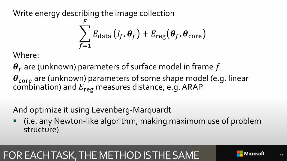
Write energy describing the image collection

𝑓=1

𝐹

𝐸data 𝐼𝑓 , 𝜽𝑓 + 𝐸reg 𝜽𝑓 , 𝜽core

Where:

𝜽𝑓 are (unknown) parameters of surface model in frame 𝑓

𝜽core are (unknown) parameters of some shape model (e.g. linear combination) and 𝐸reg measures distance, e.g. ARAP

And optimize it using Levenberg-Marquardt

(i.e. any Newton-like algorithm, making maximum use of problem structure)

FOR EACH TASK, THE METHOD IS THE SAME 37

So, you can do lots of things by “fitting models to data”.

How do you do it right?

Let’s look at some examples.

38

EXAMPLE: SHAPE FITTING

39

SHAPE QUIZ 40

t = 0:.01:2;

plot(cos(t)*2, sin(t));

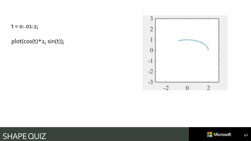
SHAPE QUIZ 41

t = 0:.01:2;

plot(cos(t)*2, sin(t));

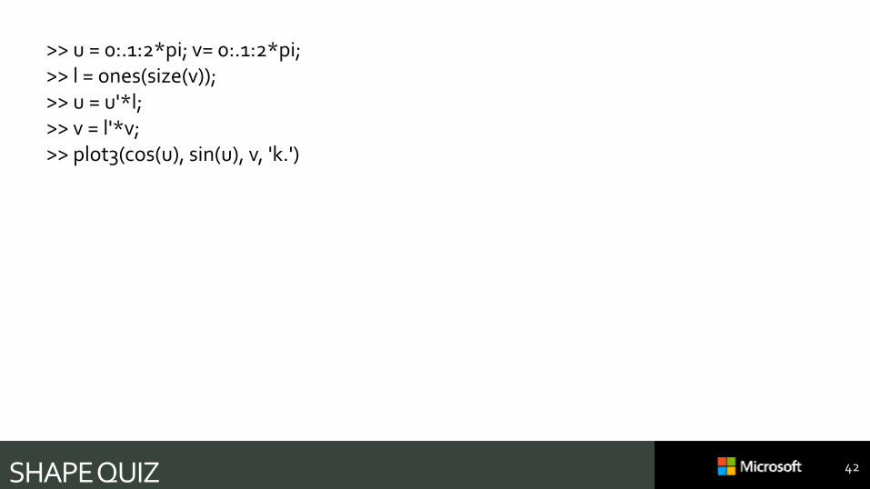
SHAPE QUIZ 42

>> u = 0:.1:2*pi; v= 0:.1:2*pi;>> l = ones(size(v));>> u = u'*l;>> v = l'*v;>> plot3(cos(u), sin(u), v, 'k.')

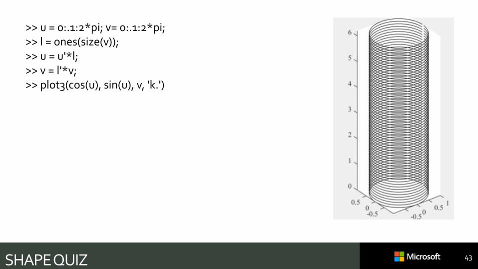
SHAPE QUIZ 43

>> u = 0:.1:2*pi; v= 0:.1:2*pi;>> l = ones(size(v));>> u = u'*l;>> v = l'*v;>> plot3(cos(u), sin(u), v, 'k.')

What is a shape?• Functions

• Curves

• Surfaces

44

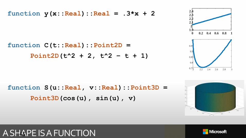
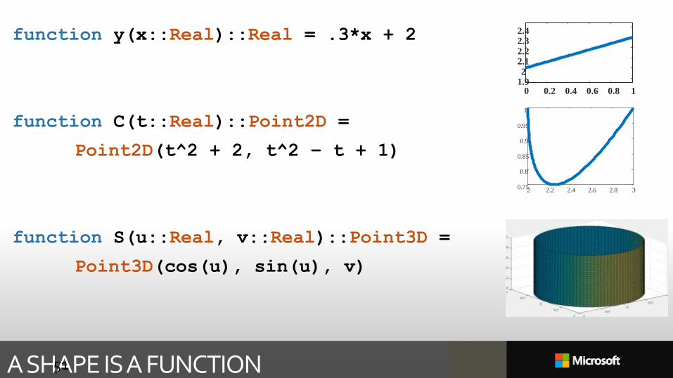
A SHAPE IS A FUNCTION

function y(x::Real)::Real = .3*x + 2

function C(t::Real)::Point2D =

Point2D(t^2 + 2, t^2 – t + 1)

function S(u::Real, v::Real)::Point3D =

Point3D(cos(u), sin(u), v)

45

2 2.2 2.4 2.6 2.8 30.75

0.8

0.85

0.9

0.95

1

0 0.2 0.4 0.6 0.8 11.92

2.12.22.32.4

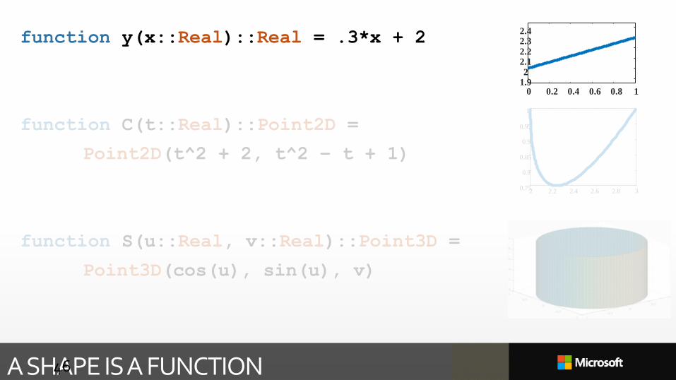
A SHAPE IS A FUNCTION

function y(x::Real)::Real = .3*x + 2

function C(t::Real)::Point2D =

Point2D(t^2 + 2, t^2 – t + 1)

function S(u::Real, v::Real)::Point3D =

Point3D(cos(u), sin(u), v)

46

2 2.2 2.4 2.6 2.8 30.75

0.8

0.85

0.9

0.95

1

0 0.2 0.4 0.6 0.8 11.92

2.12.22.32.4

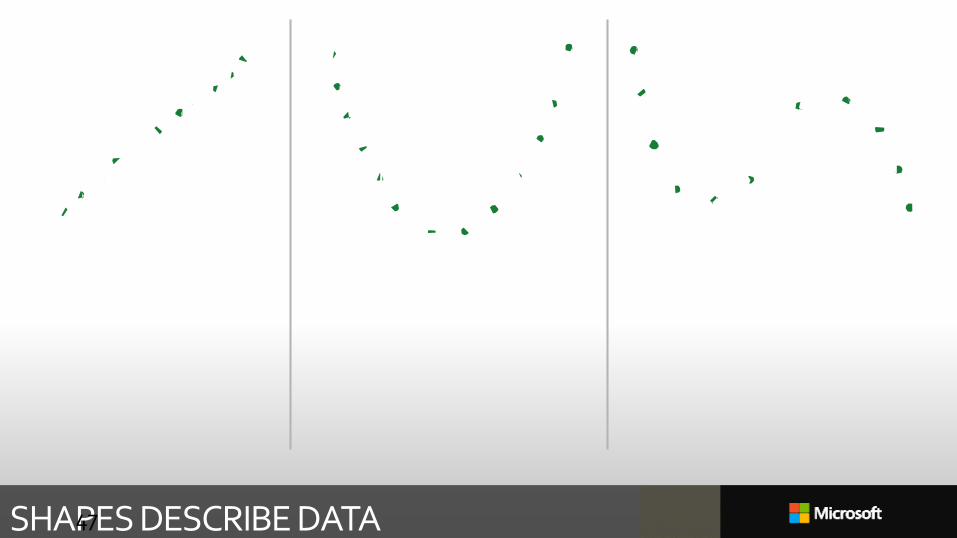
SHAPES DESCRIBE DATA47

SHAPES DESCRIBE DATA48

𝑦 = 𝑎𝑥 + 𝑏 𝑦 = 𝑎𝑥2 + 𝑏𝑥 + 𝑐 𝑦 = 𝑎𝑥3 + 𝑏𝑥2 + 𝑐𝑥 + 𝑑

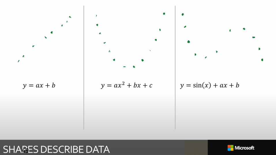
SHAPES DESCRIBE DATA49

𝑦 = 𝑎𝑥 + 𝑏 𝑦 = 𝑎𝑥2 + 𝑏𝑥 + 𝑐 𝑦 = sin 𝑥 + 𝑎𝑥 + 𝑏

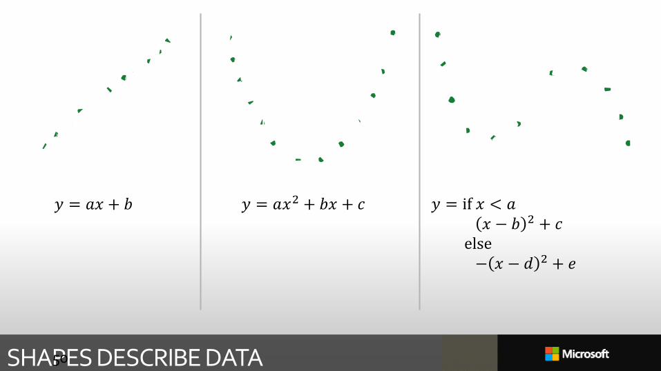
SHAPES DESCRIBE DATA50

𝑦 = 𝑎𝑥 + 𝑏 𝑦 = 𝑎𝑥2 + 𝑏𝑥 + 𝑐 𝑦 = if 𝑥 < 𝑎𝑥 − 𝑏 2 + 𝑐

else− 𝑥 − 𝑑 2 + 𝑒

A SHAPE IS A FUNCTION51

2 2.2 2.4 2.6 2.8 30.75

0.8

0.85

0.9

0.95

1

function y(x::Real)::Real = .3*x + 2

function C(t::Real)::Point2D =

Point2D(t^2 + 2, t^2 – t + 1)

function S(u::Real, v::Real)::Point3D =

Point3D(cos(u), sin(u), v)

0 0.2 0.4 0.6 0.8 11.92

2.12.22.32.4

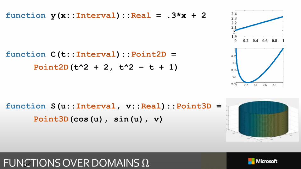
FUNCTIONS OVER DOMAINS Ω

function y(x::Interval)::Real = .3*x + 2

function C(t::Interval)::Point2D =

Point2D(t^2 + 2, t^2 – t + 1)

function S(u::Interval, v::Real)::Point3D =

Point3D(cos(u), sin(u), v)

52

2 2.2 2.4 2.6 2.8 30.75

0.8

0.85

0.9

0.95

1

0 0.2 0.4 0.6 0.8 11.92

2.12.22.32.4

0 0.2 0.4 0.6 0.8 11.92

2.12.22.32.4

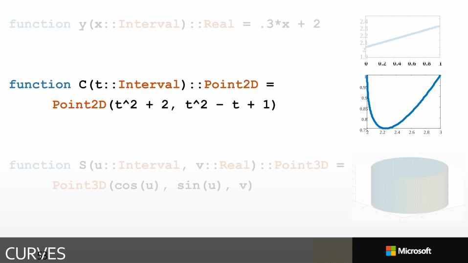
CURVES

function y(x::Interval)::Real = .3*x + 2

function C(t::Interval)::Point2D =

Point2D(t^2 + 2, t^2 – t + 1)

function S(u::Interval, v::Real)::Point3D =

Point3D(cos(u), sin(u), v)

53

2 2.2 2.4 2.6 2.8 30.75

0.8

0.85

0.9

0.95

1

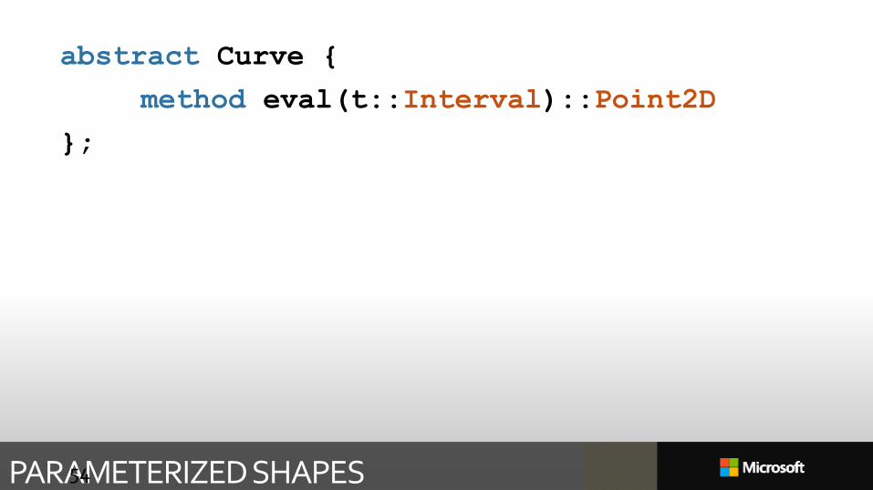
PARAMETERIZED SHAPES

abstract Curve {

method eval(t::Interval)::Point2D

};

54

PARAMETERIZED SHAPES55

2 2.2 2.4 2.6 2.8 30.75

0.8

0.85

0.9

0.95

1

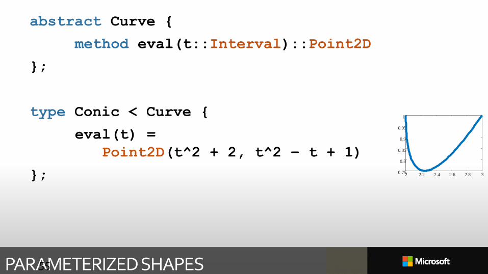
abstract Curve {

method eval(t::Interval)::Point2D

};

type Conic < Curve {

eval(t) =

Point2D(t^2 + 2, t^2 – t + 1)

};

PARAMETERIZED SHAPES

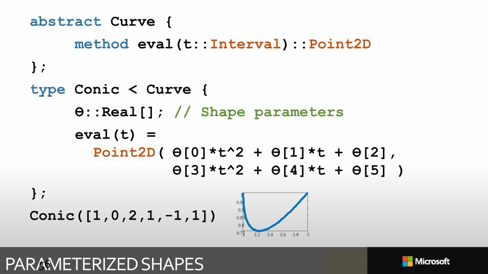
abstract Curve {

method eval(t::Interval)::Point2D

};

type Conic < Curve {

ϴ::Real[]; // Shape parameters

eval(t) =

Point2D( ϴ[0]*t^2 + ϴ[1]*t + ϴ[2],

ϴ[3]*t^2 + ϴ[4]*t + ϴ[5] )

};

Conic([1,0,2,1,-1,1])

56

2 2.2 2.4 2.6 2.8 30.75

0.8

0.85

0.9

0.95

1

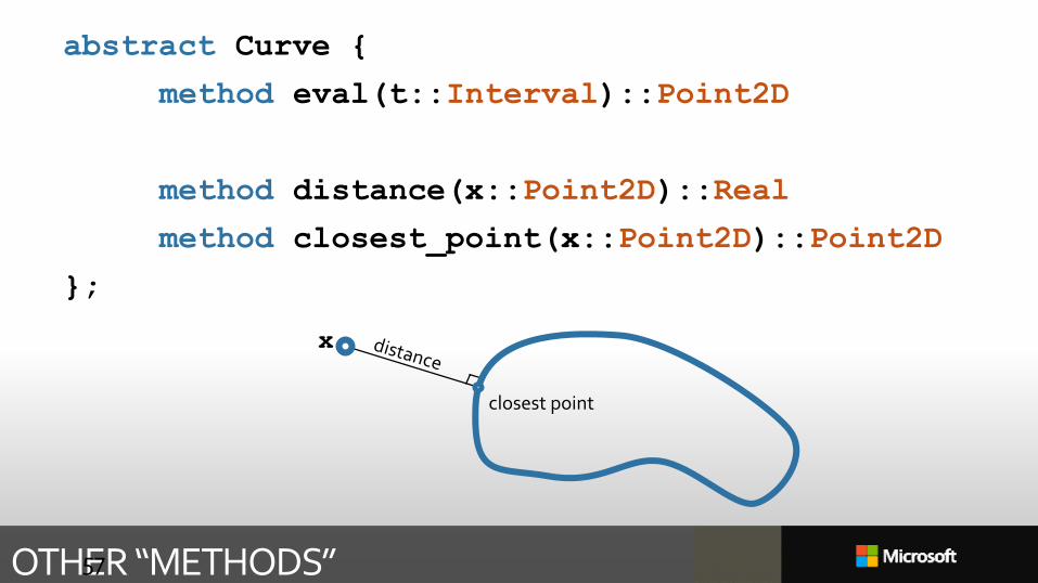
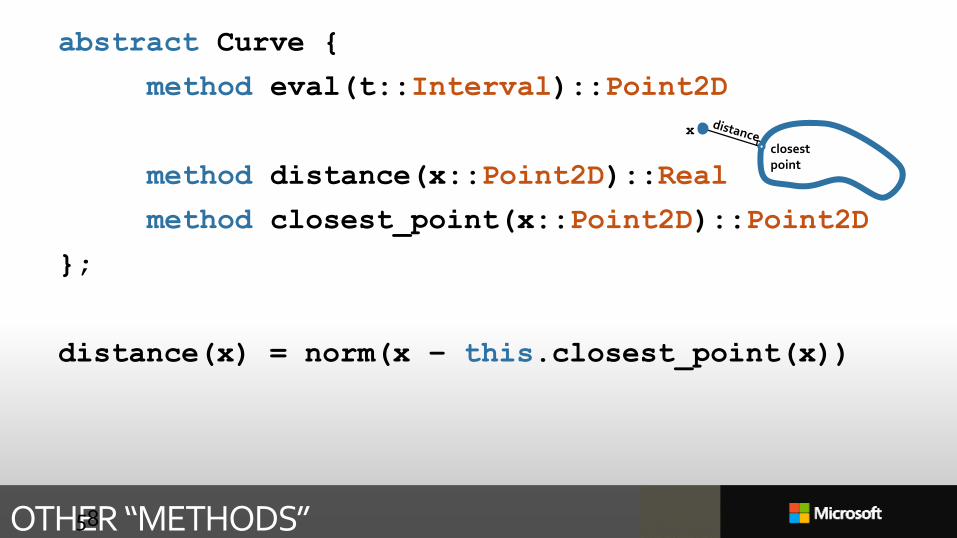
OTHER “METHODS”

abstract Curve {

method eval(t::Interval)::Point2D

method distance(x::Point2D)::Real

method closest_point(x::Point2D)::Point2D

};

57

closest point

x

OTHER “METHODS”

abstract Curve {

method eval(t::Interval)::Point2D

method distance(x::Point2D)::Real

method closest_point(x::Point2D)::Point2D

};

distance(x) = norm(x – this.closest_point(x))

58

closest point

x

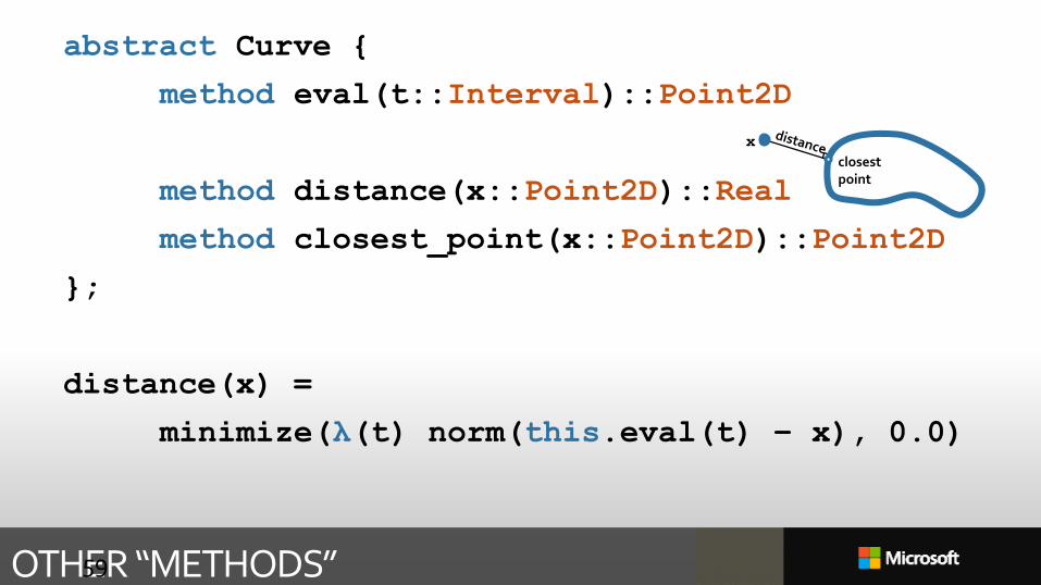
OTHER “METHODS”

abstract Curve {

method eval(t::Interval)::Point2D

method distance(x::Point2D)::Real

method closest_point(x::Point2D)::Point2D

};

distance(x) =

minimize(λ(t) norm(this.eval(t) – x), 0.0)

59

closest point

x

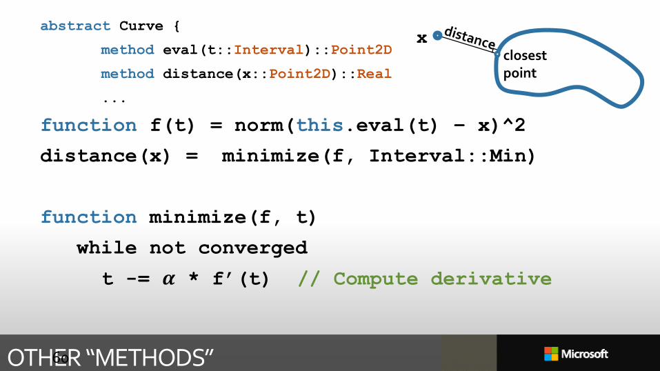
OTHER “METHODS”

abstract Curve {

method eval(t::Interval)::Point2D

method distance(x::Point2D)::Real

...

function f(t) = norm(this.eval(t) – x)^2

distance(x) = minimize(f, Interval::Min)

function minimize(f, t)

while not converged

t -= 𝜶 * f’(t) // Compute derivative

60

closest point

x

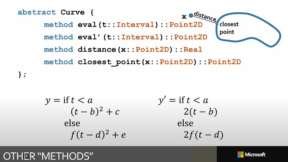
OTHER “METHODS”

abstract Curve {

method eval(t::Interval)::Point2D

method eval’(t::Interval)::Point2D

method distance(x::Point2D)::Real

method closest_point(x::Point2D)::Point2D

};

61

closest point

x

𝑦 = if 𝑡 < 𝑎𝑡 − 𝑏 2 + 𝑐

else𝑓 𝑡 − 𝑑 2 + 𝑒

𝑦′ = if 𝑡 < 𝑎2(𝑡 − 𝑏)

else2𝑓(𝑡 − 𝑑)

Shape, meet thy data

62

min𝜃

𝑛=1

𝑁

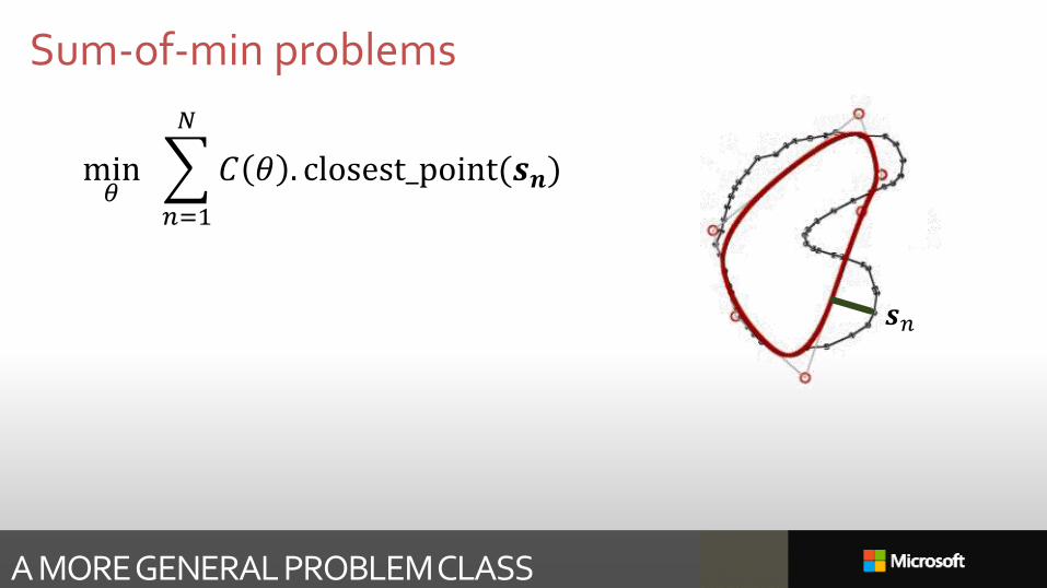
𝐶 𝜃 . closest_point(𝒔𝒏)

Sum-of-min problems

𝒔𝑛

A MORE GENERAL PROBLEM CLASS

AN EXEMPLARY PROBLEM

64

“Based on a true story”, not necessarily historically accurate

Note well: this problem is a good proxy for much more realistic problems:

1. Stereo camera calibration

2. Multiple-camera bundle adjustment

3. Surface fitting, e.g. subdivision surfaces to range data, realtime hand tracking

4. Matrix completion

5. Image denoising.

[Inspired by Neil Lawrence’s professorial inaugural]

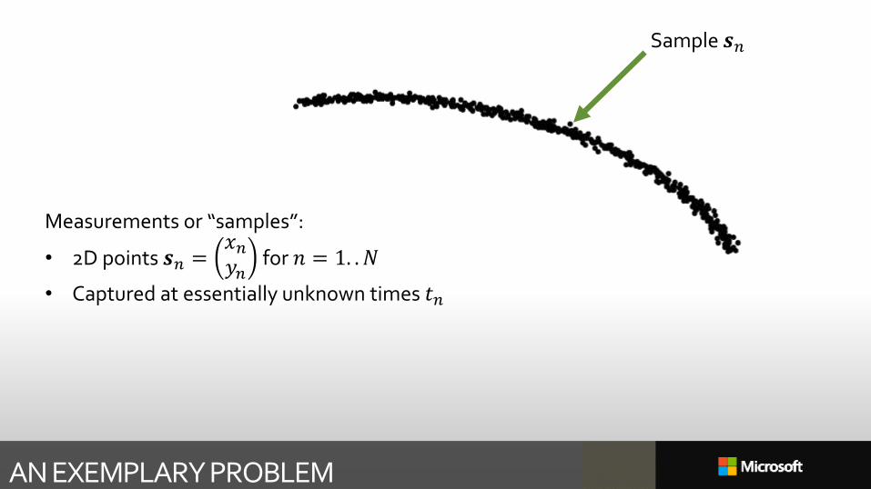
AN EXEMPLARY PROBLEM

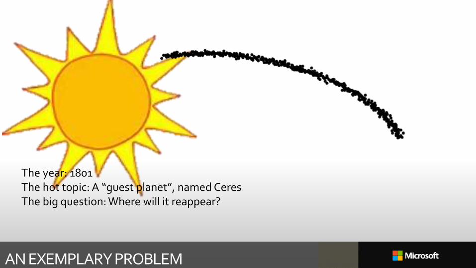
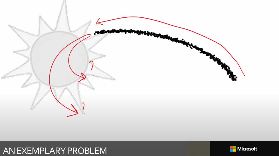
The year: 1801The hot topic: A “guest planet”, named CeresThe big question: Where will it reappear?

AN EXEMPLARY PROBLEM

AN EXEMPLARY PROBLEM

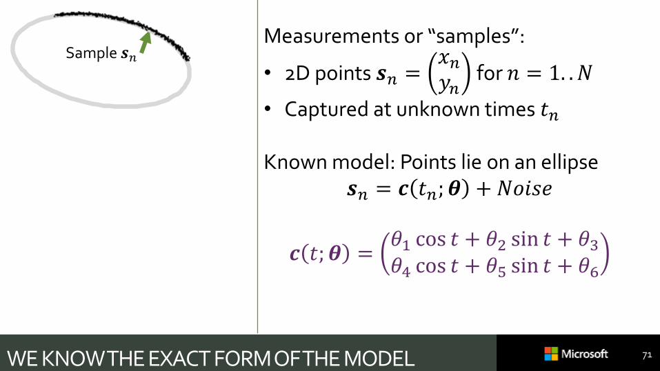
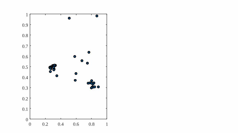
Measurements or “samples”:

• 2D points 𝒔𝑛 =𝑥𝑛𝑦𝑛

for 𝑛 = 1. . 𝑁

• Captured at essentially unknown times 𝑡𝑛

Sample 𝒔𝑛

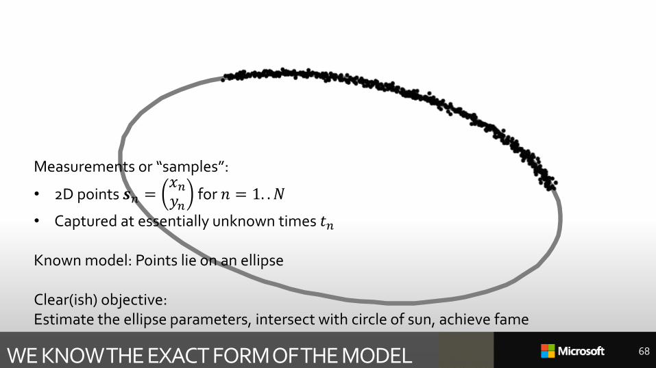
WE KNOW THE EXACT FORM OF THE MODEL 68

Measurements or “samples”:

• 2D points 𝒔𝑛 =𝑥𝑛𝑦𝑛

for 𝑛 = 1. . 𝑁

• Captured at essentially unknown times 𝑡𝑛

Known model: Points lie on an ellipse

Clear(ish) objective: Estimate the ellipse parameters, intersect with circle of sun, achieve fame

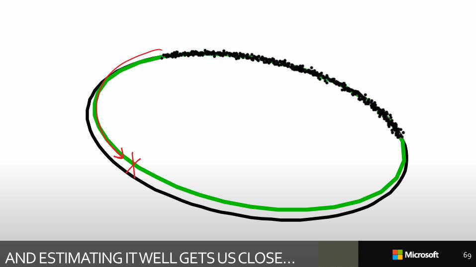
AND ESTIMATING IT WELL GETS US CLOSE… 69

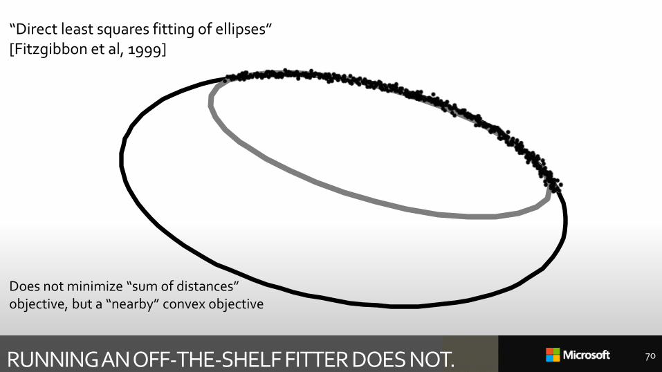
RUNNING AN OFF-THE-SHELF FITTER DOES NOT. 70

“Direct least squares fitting of ellipses”[Fitzgibbon et al, 1999]

Does not minimize “sum of distances” objective, but a “nearby” convex objective

WE KNOW THE EXACT FORM OF THE MODEL 71

Measurements or “samples”:

• 2D points 𝒔𝑛 =𝑥𝑛𝑦𝑛

for 𝑛 = 1. . 𝑁

• Captured at unknown times 𝑡𝑛

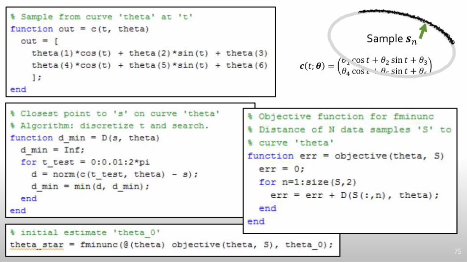
Known model: Points lie on an ellipse𝒔𝑛 = 𝒄 𝑡𝑛; 𝜽 + 𝑁𝑜𝑖𝑠𝑒

𝒄 𝑡; 𝜽 =𝜃1 cos 𝑡 + 𝜃2 sin 𝑡 + 𝜃3𝜃4 cos 𝑡 + 𝜃5 sin 𝑡 + 𝜃6

Sample 𝒔𝑛

A PARAMETRIC FUNCTION AND A CURVE 72

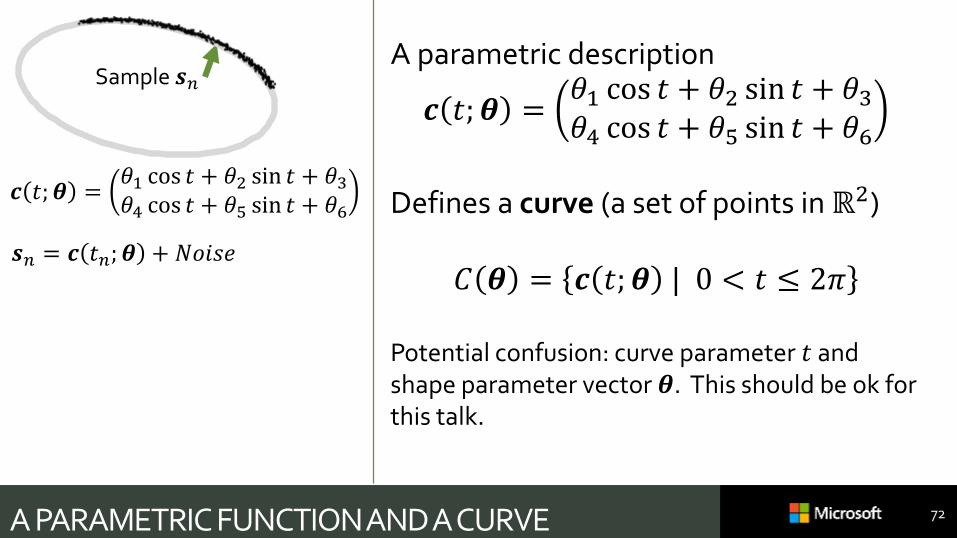
A parametric description

𝒄 𝑡; 𝜽 =𝜃1 cos 𝑡 + 𝜃2 sin 𝑡 + 𝜃3𝜃4 cos 𝑡 + 𝜃5 sin 𝑡 + 𝜃6

Defines a curve (a set of points in ℝ2)

𝐶 𝜽 = 𝒄 𝑡; 𝜽 | 0 < 𝑡 ≤ 2𝜋

Potential confusion: curve parameter 𝑡 and shape parameter vector 𝜽. This should be ok for this talk.

Sample 𝒔𝑛

𝒔𝑛 = 𝒄 𝑡𝑛; 𝜽 + 𝑁𝑜𝑖𝑠𝑒

𝒄 𝑡; 𝜽 =𝜃1 cos 𝑡 + 𝜃2 sin 𝑡 + 𝜃3𝜃4 cos 𝑡 + 𝜃5 sin 𝑡 + 𝜃6

DISTANCES AND CLOSEST POINTS 73

Sample 𝒔𝑛

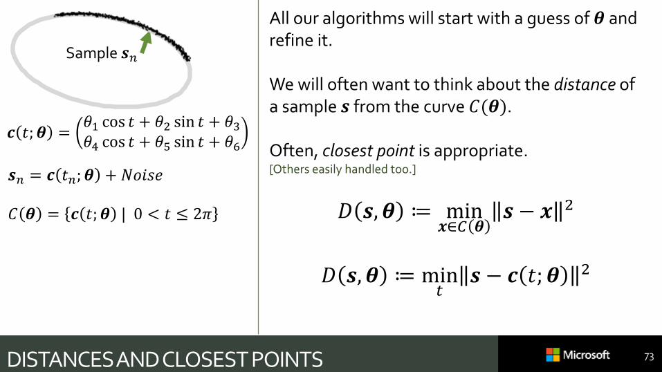
All our algorithms will start with a guess of 𝜽 and refine it.

We will often want to think about the distance of a sample 𝒔 from the curve 𝐶(𝜽).

Often, closest point is appropriate. [Others easily handled too.]

𝐷 𝒔, 𝜽 ≔ min𝒙∈𝐶 𝜽

𝒔 − 𝒙 2

𝐷 𝒔, 𝜽 ≔ min𝑡

𝒔 − 𝒄 𝑡; 𝜽 2

𝒔𝑛 = 𝒄 𝑡𝑛; 𝜽 + 𝑁𝑜𝑖𝑠𝑒

𝒄 𝑡; 𝜽 =𝜃1 cos 𝑡 + 𝜃2 sin 𝑡 + 𝜃3𝜃4 cos 𝑡 + 𝜃5 sin 𝑡 + 𝜃6

𝐶 𝜽 = 𝒄 𝑡; 𝜽 | 0 < 𝑡 ≤ 2𝜋

A BETTER ESTIMATE 74

Sample 𝒔𝑛

𝒔𝑛 = 𝒄 𝑡𝑛; 𝜽 + 𝑁𝑜𝑖𝑠𝑒

𝒄 𝑡; 𝜽 =𝜃1 cos 𝑡 + 𝜃2 sin 𝑡 + 𝜃3𝜃4 cos 𝑡 + 𝜃5 sin 𝑡 + 𝜃6

𝐶 𝜽 = 𝒄 𝑡; 𝜽 | 0 < 𝑡 ≤ 2𝜋

𝐷 𝒔, 𝜽 ≔ min𝑡

𝒔 − 𝒄 𝑡; 𝜽 2

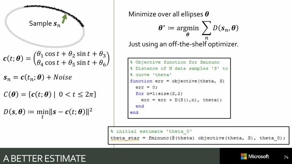
Minimize over all ellipses 𝜽

𝜽∗ ≔ argmin𝜽

𝑛

𝐷 𝒔𝑛, 𝜽

Just using an off-the-shelf optimizer.

75

𝒄 𝑡; 𝜽 =𝜃1 cos 𝑡 + 𝜃2 sin 𝑡 + 𝜃3𝜃4 cos 𝑡 + 𝜃5 sin 𝑡 + 𝜃6

Sample 𝒔𝑛

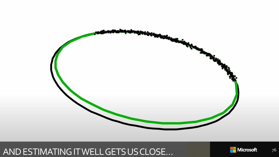
AND ESTIMATING IT WELL GETS US CLOSE… 76

SO ARE WE DONE YET?

We have an accurate solution Certainly better than the “closed form” algorithm, which minimized a “nearby” convex

objective.

All we need to worry about now is speed… If you take 3 weeks to make a prediction, someone else will get the fame.

Speed is everything. If speed didn’t matter, you would just use random search.

Strategies to speed it up Attack the inner loop

Remove discrete minimization in 𝐷(𝒔, 𝜽)

Analyse the problem again

Understand our tools: ‘fminunc’, or whatever we’re using

Compute analytic derivatives

77

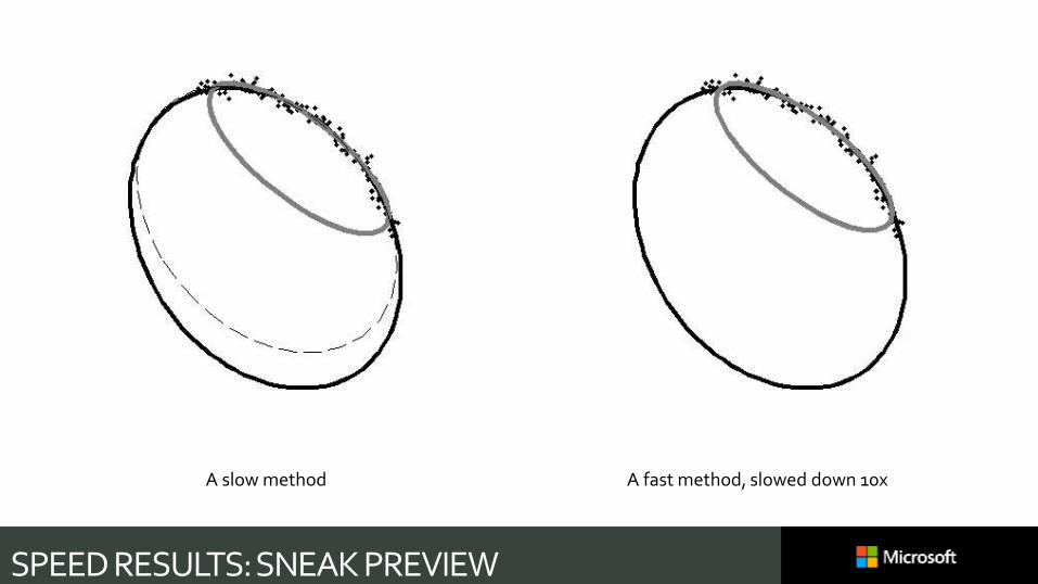
SPEED RESULTS: SNEAK PREVIEW

A slow method A fast method, slowed down 10x

SPEEDUP 1: ATTACK THE INNER LOOP

79

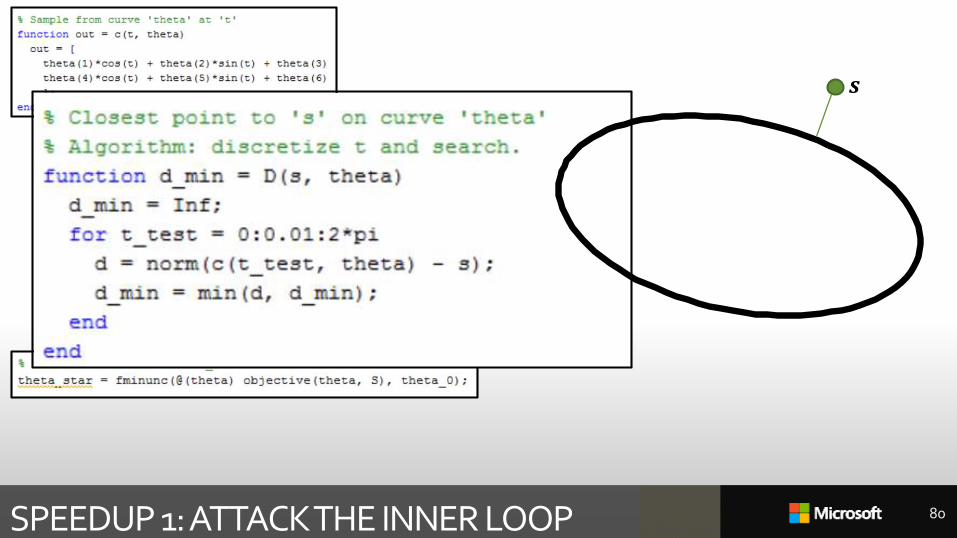
SPEEDUP 1: ATTACK THE INNER LOOP 80

𝒔

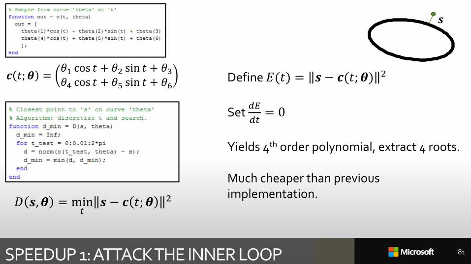
SPEEDUP 1: ATTACK THE INNER LOOP 81

𝒔

𝐷 𝒔, 𝜽 = min𝑡

𝒔 − 𝒄 𝑡; 𝜽 2

Define 𝐸(𝑡) = 𝒔 − 𝒄(𝑡; 𝜽) 2

Set 𝑑𝐸

𝑑𝑡= 0

Yields 4th order polynomial, extract 4 roots.

Much cheaper than previous implementation.

𝒄 𝑡; 𝜽 =𝜃1 cos 𝑡 + 𝜃2 sin 𝑡 + 𝜃3𝜃4 cos 𝑡 + 𝜃5 sin 𝑡 + 𝜃6

SPEEDUP 2: ANALYSE THE PROBLEM

82

LOOK AT THE PROBLEM AGAIN 83

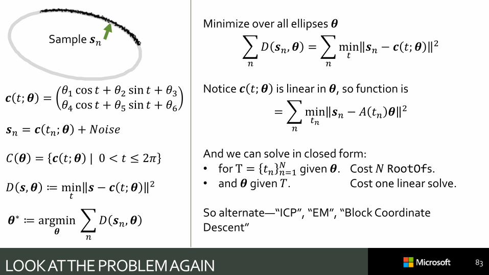
Sample 𝒔𝑛

𝒔𝑛 = 𝒄 𝑡𝑛; 𝜽 + 𝑁𝑜𝑖𝑠𝑒

𝒄 𝑡; 𝜽 =𝜃1 cos 𝑡 + 𝜃2 sin 𝑡 + 𝜃3𝜃4 cos 𝑡 + 𝜃5 sin 𝑡 + 𝜃6

𝐶 𝜽 = 𝒄 𝑡; 𝜽 | 0 < 𝑡 ≤ 2𝜋

𝐷 𝒔, 𝜽 ≔ min𝑡

𝒔 − 𝒄 𝑡; 𝜽 2

Minimize over all ellipses 𝜽

𝑛

𝐷 𝒔𝑛, 𝜽 =

𝑛

min𝑡

𝒔𝑛 − 𝒄 𝑡; 𝜽 2

Notice 𝒄 𝑡; 𝜽 is linear in 𝜽, so function is

=

𝑛

min𝑡𝑛

𝒔𝑛 − 𝐴 𝑡𝑛 𝜽 2

And we can solve in closed form:• for T = 𝑡𝑛 𝑛=1

𝑁 given 𝜽. Cost 𝑁 RootOfs.• and 𝜽 given 𝑇. Cost one linear solve.

So alternate—“ICP”, “EM”, “Block Coordinate Descent”

𝜽∗ ≔ argmin𝜽

𝑛

𝐷 𝒔𝑛, 𝜽

bad decision…

84

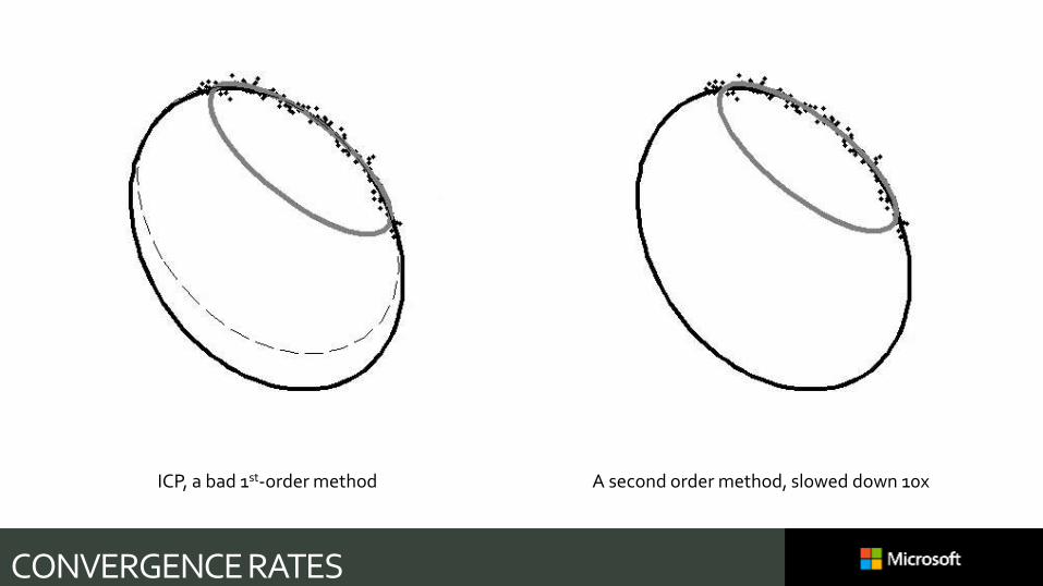
CONVERGENCE RATES

ICP, a bad 1st-order method A second order method, slowed down 10x

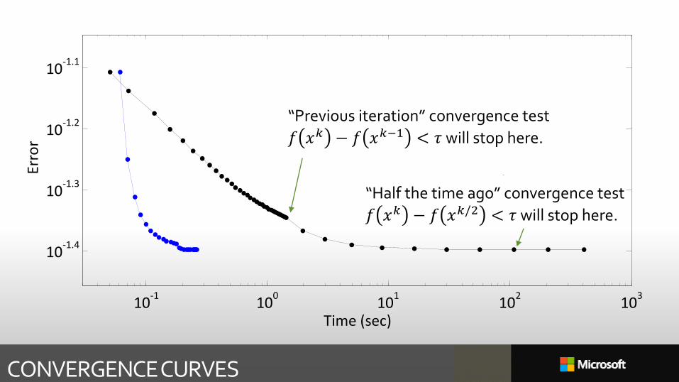
CONVERGENCE CURVES

10-1

100

101

102

103

10-1.4

10-1.3

10-1.2

10-1.1

Time (sec)

Erro

r

“Previous iteration” convergence test

𝑓 𝑥𝑘 − 𝑓 𝑥𝑘−1 < 𝜏 will stop here.

“Half the time ago” convergence test

𝑓 𝑥𝑘 − 𝑓 𝑥𝑘/2 < 𝜏 will stop here.

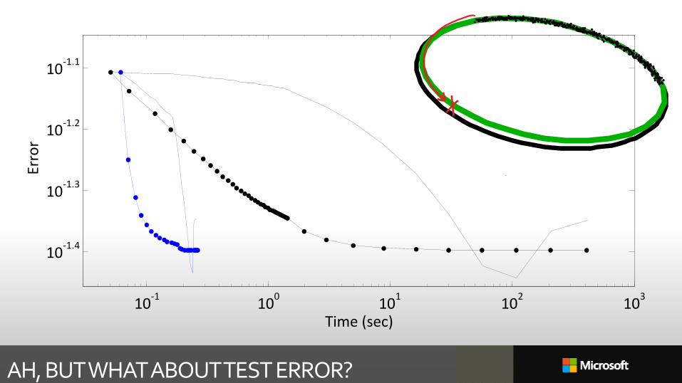
AH, BUT WHAT ABOUT TEST ERROR?

10-1

100

101

102

103

10-1.4

10-1.3

10-1.2

10-1.1

Time (sec)

Erro

r

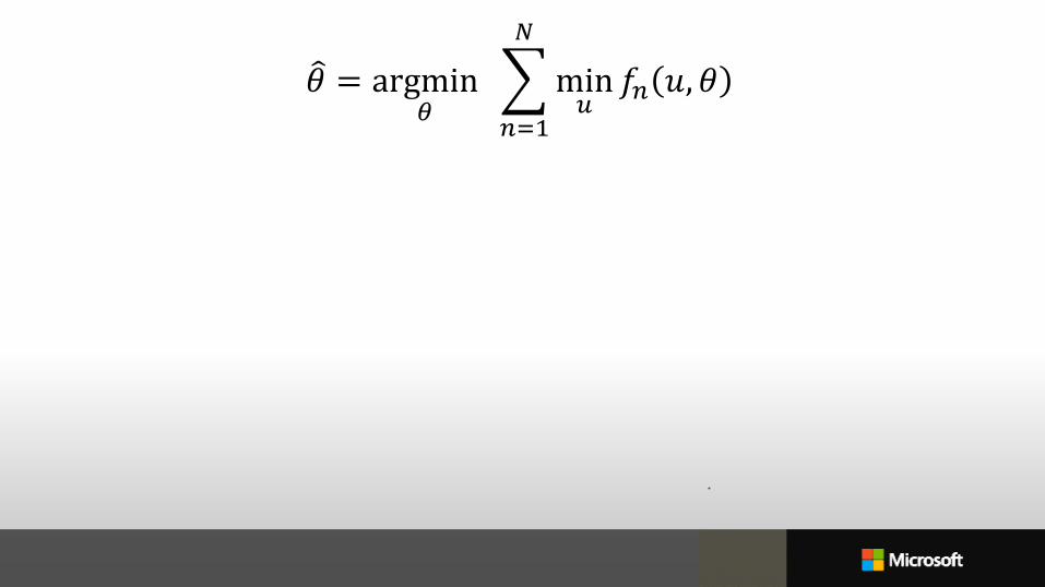
𝜃 = argmin𝜃

𝑛=1

𝑁

min𝑢

𝑓𝑛 𝑢, 𝜃

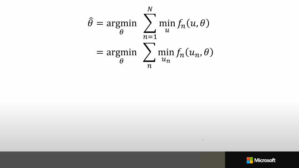
𝜃 = argmin𝜃

𝑛=1

𝑁

min𝑢

𝑓𝑛 𝑢, 𝜃

= argmin𝜃

𝑛

min𝑢𝑛

𝑓𝑛 𝑢𝑛, 𝜃

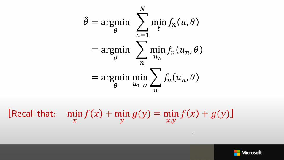
𝜃 = argmin𝜃

𝑛=1

𝑁

min𝑡𝑓𝑛 𝑢, 𝜃

= argmin𝜃

𝑛

min𝑢𝑛

𝑓𝑛 𝑢𝑛, 𝜃

= argmin𝜃

min𝑢1..𝑁

𝑛

𝑓𝑛 𝑢𝑛, 𝜃

[Recall that: min𝑥

𝑓 𝑥 +min𝑦

𝑔(𝑦) = min𝑥,𝑦

𝑓 𝑥 + 𝑔(𝑦)]

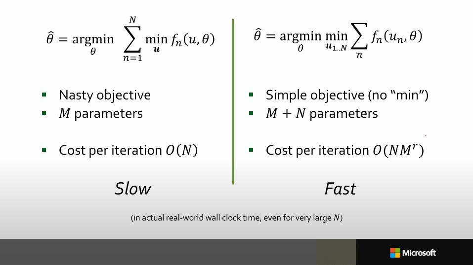
SUMMARY: TWO METHODS, SAME OBJECTIVE𝜃 = argmin𝜃

𝑛=1

𝑁

min𝒖

𝑓𝑛 𝑢, 𝜃

Nasty objective

𝑀 parameters

Cost per iteration 𝑂 𝑁

Slow

𝜃 = argmin𝜃

min𝒖1..𝑁

𝑛

𝑓𝑛 𝑢𝑛, 𝜃

Simple objective (no “min”)

𝑀 +𝑁 parameters

Cost per iteration 𝑂(𝑁𝑀𝑟)

Fast

(in actual real-world wall clock time, even for very large 𝑁)

CONVERGENCE RATES

ICP, a bad 1st-order method A second order method, slowed down 10x

SPEEDUP 3: UNDERSTAND OUR TOOLS

93

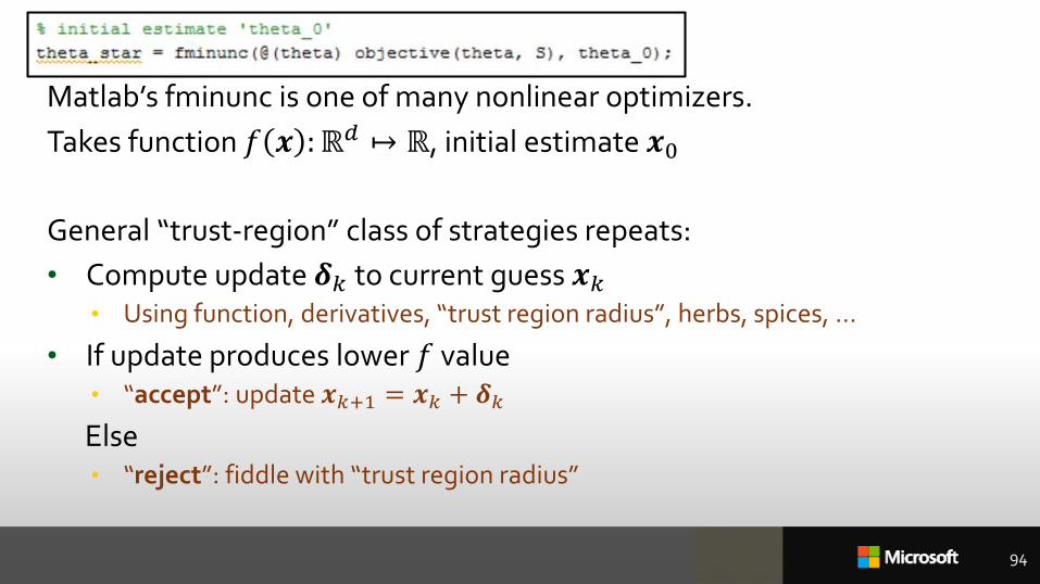
Matlab’s fminunc is one of many nonlinear optimizers.

Takes function 𝑓 𝒙 :ℝ𝑑 ↦ ℝ, initial estimate 𝒙0

General “trust-region” class of strategies repeats:

• Compute update 𝜹𝑘 to current guess 𝒙𝑘• Using function, derivatives, “trust region radius”, herbs, spices, …

• If update produces lower 𝑓 value• “accept”: update 𝒙𝑘+1 = 𝒙𝑘 + 𝜹𝑘

Else • “reject”: fiddle with “trust region radius”

94

ASIDE…

CONTINUOUS OPTIMIZATION

Andrew FitzgibbonMicrosoft Research Cambridge

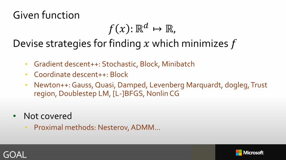
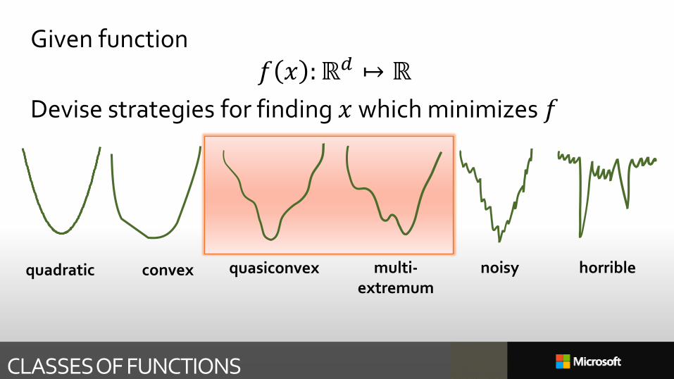
GOAL

Given function𝑓 𝑥 :ℝ𝑑 ↦ ℝ,

Devise strategies for finding 𝑥 which minimizes 𝑓

• Gradient descent++: Stochastic, Block, Minibatch

• Coordinate descent++: Block

• Newton++: Gauss, Quasi, Damped, Levenberg Marquardt, dogleg, Trust region, Doublestep LM, [L-]BFGS, Nonlin CG

• Not covered• Proximal methods: Nesterov, ADMM…

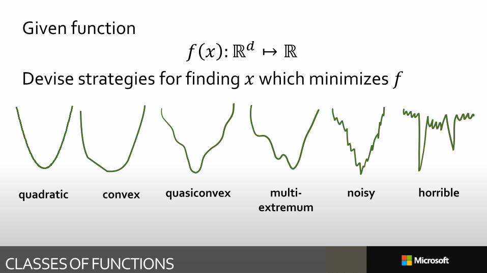
CLASSES OF FUNCTIONS

quadratic convex quasiconvex multi-extremum

noisy horrible

Given function𝑓 𝑥 :ℝ𝑑 ↦ ℝ

Devise strategies for finding 𝑥 which minimizes 𝑓

CLASSES OF FUNCTIONS

quadratic convex quasiconvex multi-extremum

noisy horrible

Given function𝑓 𝑥 :ℝ𝑑 ↦ ℝ

Devise strategies for finding 𝑥 which minimizes 𝑓

99

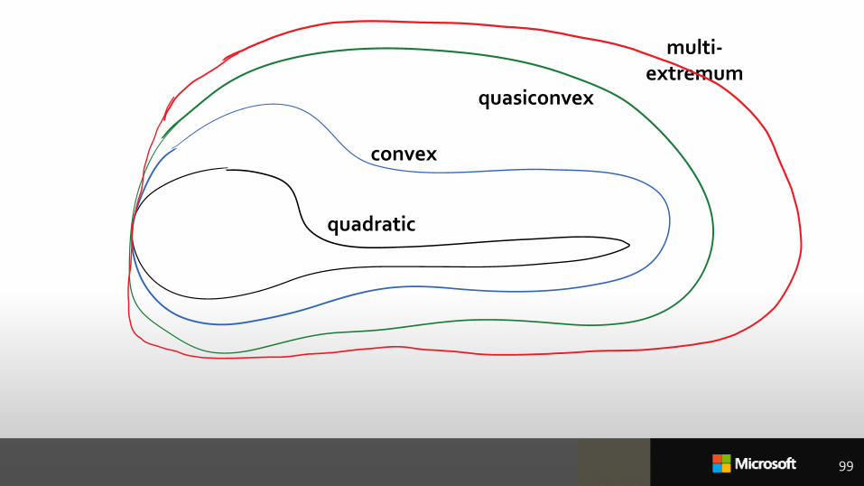
quadratic

convex

quasiconvex

multi-extremum

100

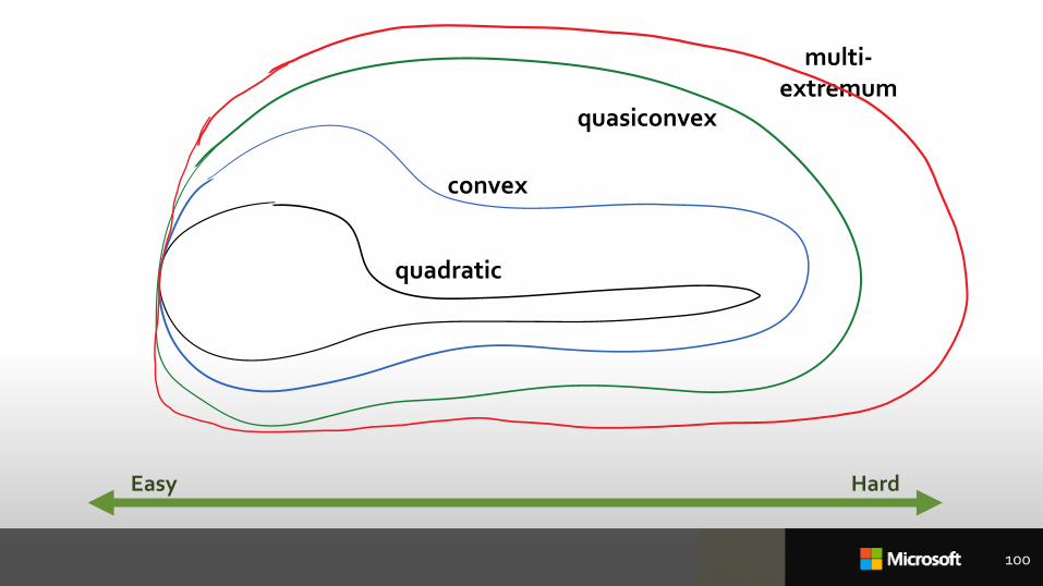
quadratic

convex

quasiconvex

multi-extremum

Easy Hard

DERIVATIVES

Fast minimization depends on derivatives

101

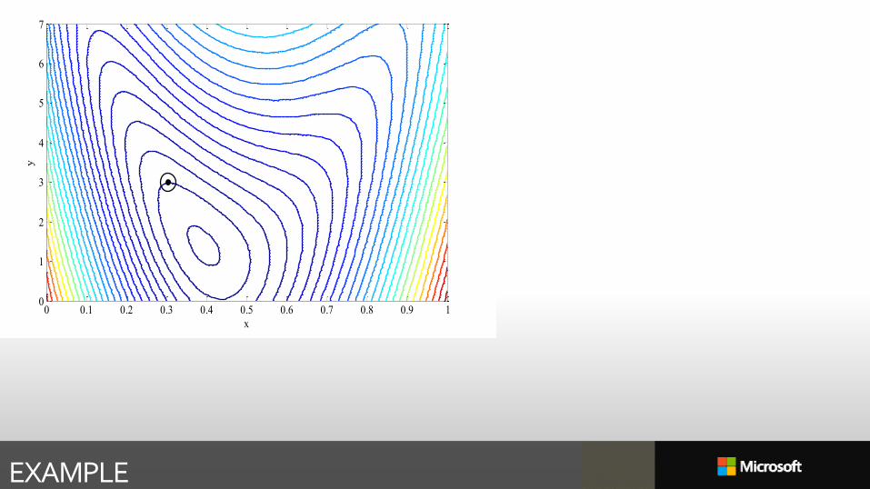
EXAMPLE

x

y

0 0.1 0.2 0.3 0.4 0.5 0.6 0.7 0.8 0.9 10

1

2

3

4

5

6

7

EXAMPLE

x

y

0 0.1 0.2 0.3 0.4 0.5 0.6 0.7 0.8 0.9 10

1

2

3

4

5

6

7

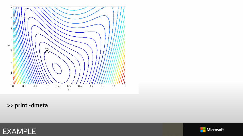
>> print -dmeta

EXAMPLE

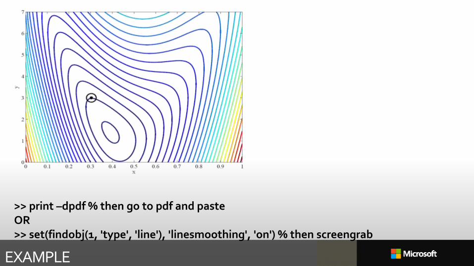
>> print –dpdf % then go to pdf and pasteOR>> set(findobj(1, 'type', 'line'), 'linesmoothing', 'on') % then screengrab

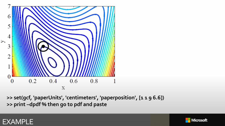
EXAMPLE

>> set(gcf, 'paperUnits', 'centimeters', 'paperposition', [1 1 9 6.6])>> print –dpdf % then go to pdf and paste

SWITCH TO MATLAB…

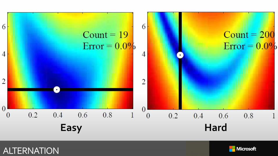
ALTERNATION

Easy Hard

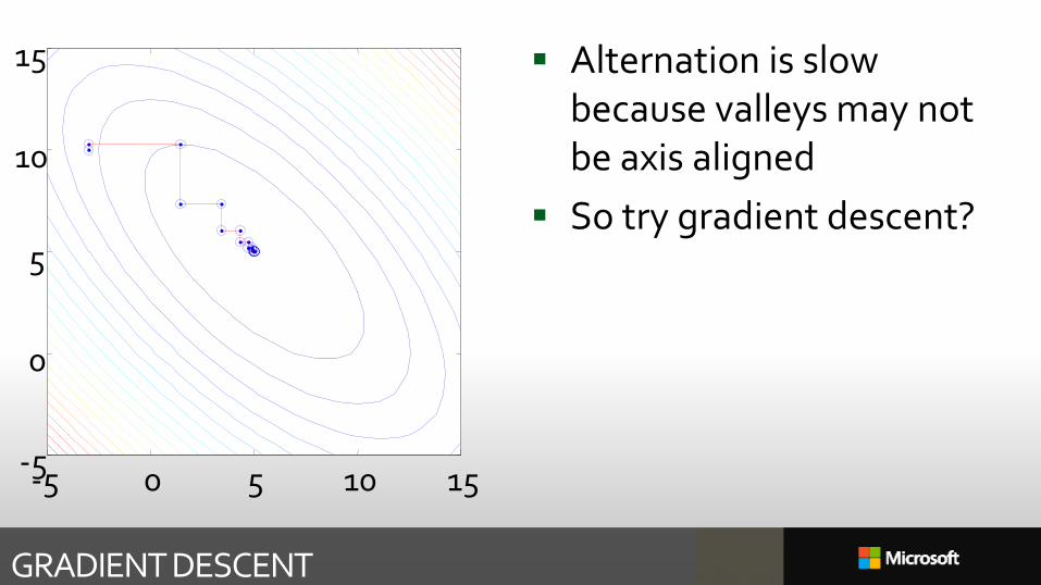
GRADIENT DESCENT

Alternation is slow because valleys may not be axis aligned

So try gradient descent?

-5 0 5 10 15-5

0

5

10

15

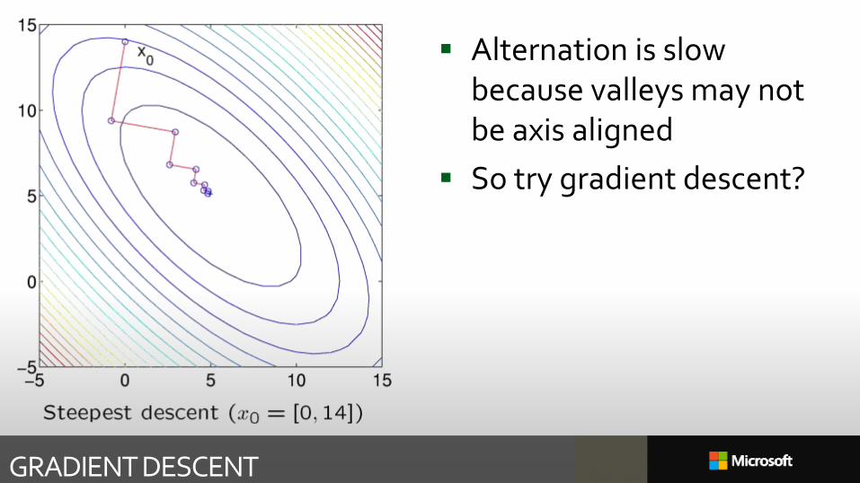
GRADIENT DESCENT

Alternation is slow because valleys may not be axis aligned

So try gradient descent?

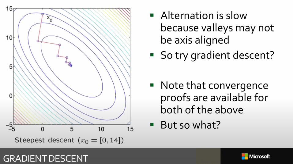
GRADIENT DESCENT

Alternation is slow because valleys may not be axis aligned

So try gradient descent?

Note that convergence proofs are available for both of the above

But so what?

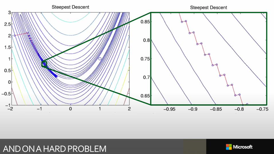
AND ON A HARD PROBLEM

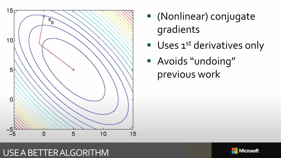
USE A BETTER ALGORITHM

(Nonlinear) conjugate gradients

Uses 1st derivatives only

Avoids “undoing” previous work

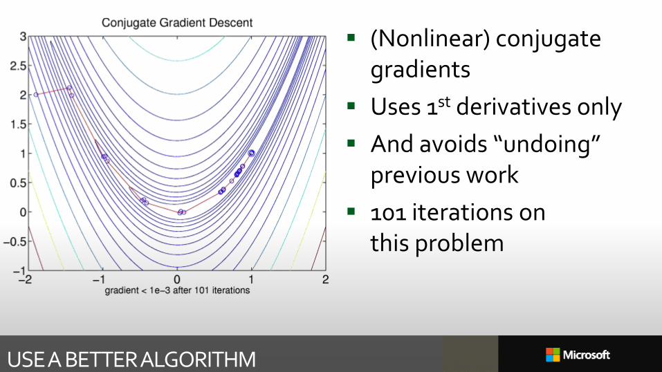
USE A BETTER ALGORITHM

(Nonlinear) conjugate gradients

Uses 1st derivatives only

And avoids “undoing” previous work

101 iterations on this problem

BUT WE CAN DO BETTER…

USE SECOND DERIVATIVES…

Starting with 𝒙 how can I choose 𝜹so that 𝑓 𝒙 + 𝜹 is better than 𝑓(𝒙)?

So computemin𝜹∈ℝ𝑑

𝑓 𝒙 + 𝜹

But hang on, that’s the same problem we were trying to solve?

USE SECOND DERIVATIVES…

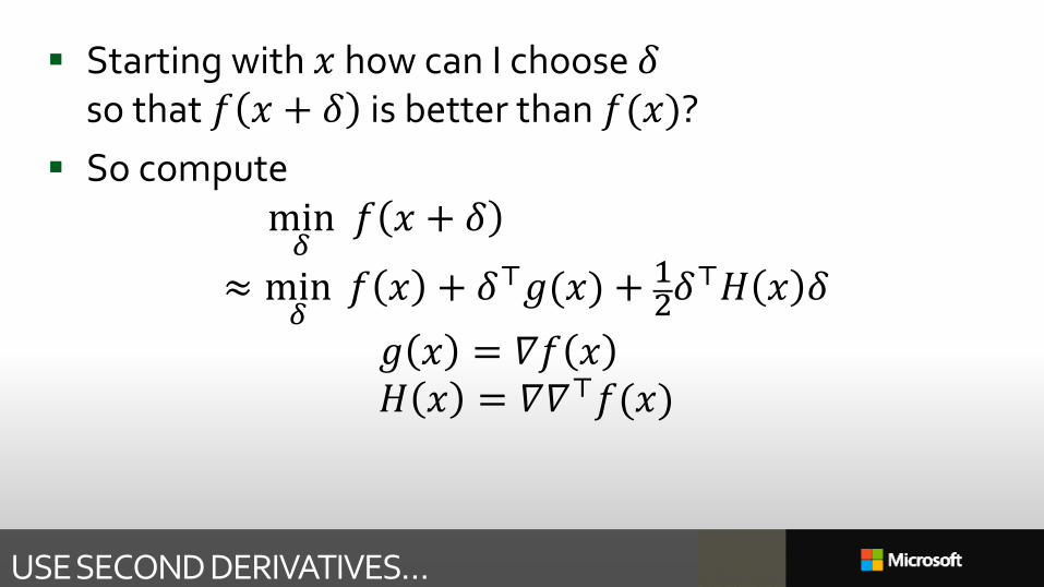
Starting with 𝑥 how can I choose 𝛿so that 𝑓 𝑥 + 𝛿 is better than 𝑓(𝑥)?

So computemin𝛿

𝑓 𝑥 + 𝛿

≈ min𝛿

𝑓 𝑥 + 𝛿⊤𝑔(𝑥) + 12𝛿

⊤𝐻 𝑥 𝛿

𝑔 𝑥 = 𝛻𝑓 𝑥𝐻 𝑥 = 𝛻𝛻⊤𝑓(𝑥)

USE SECOND DERIVATIVES…

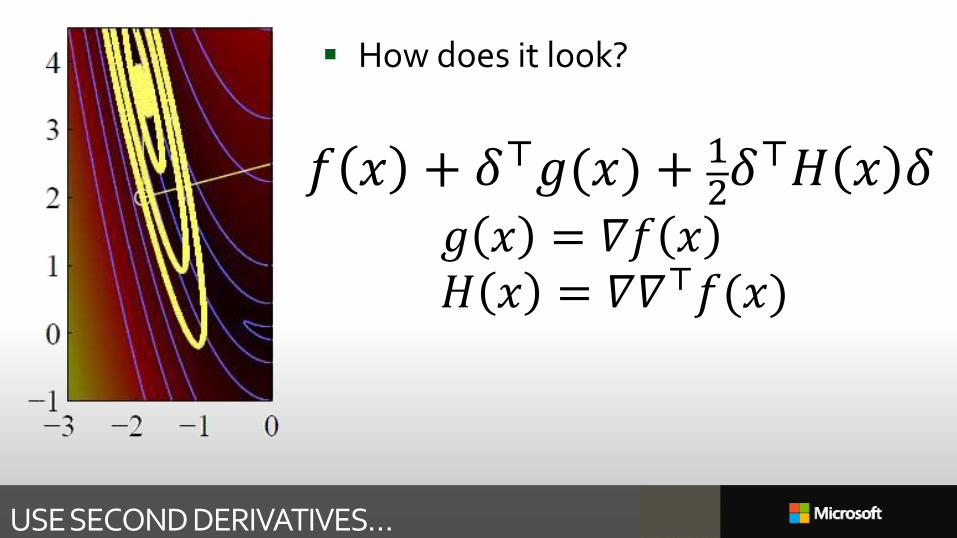
How does it look?

𝑓 𝑥 + 𝛿⊤𝑔(𝑥) + 12𝛿⊤𝐻 𝑥 𝛿

𝑔 𝑥 = 𝛻𝑓 𝑥𝐻 𝑥 = 𝛻𝛻⊤𝑓(𝑥)

USE SECOND DERIVATIVES…

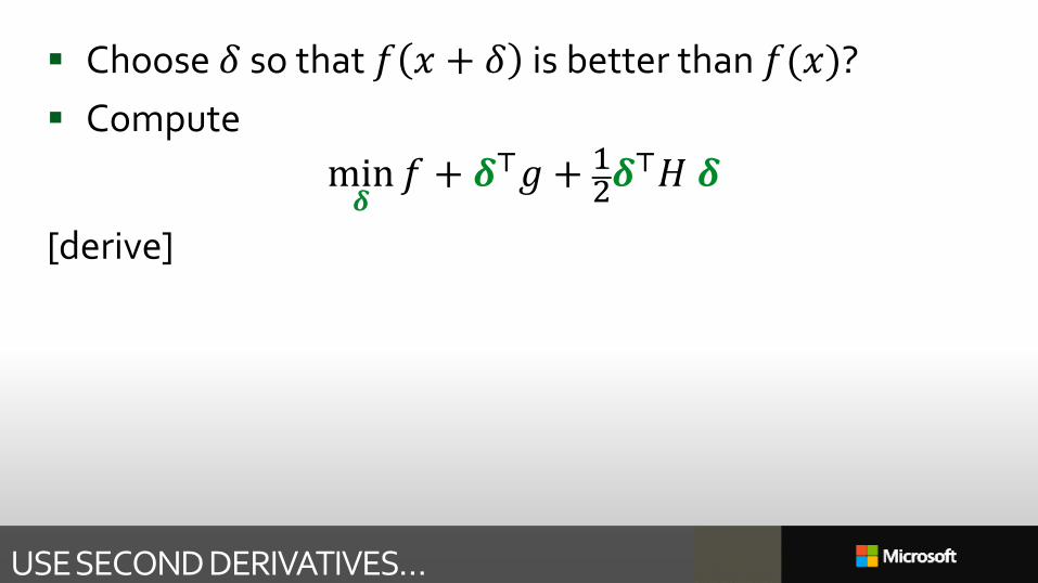
Choose 𝛿 so that 𝑓 𝑥 + 𝛿 is better than 𝑓(𝑥)?

Compute

min𝜹

𝑓 + 𝜹⊤𝑔 + 12𝜹

⊤𝐻 𝜹

[derive]

USE SECOND DERIVATIVES…

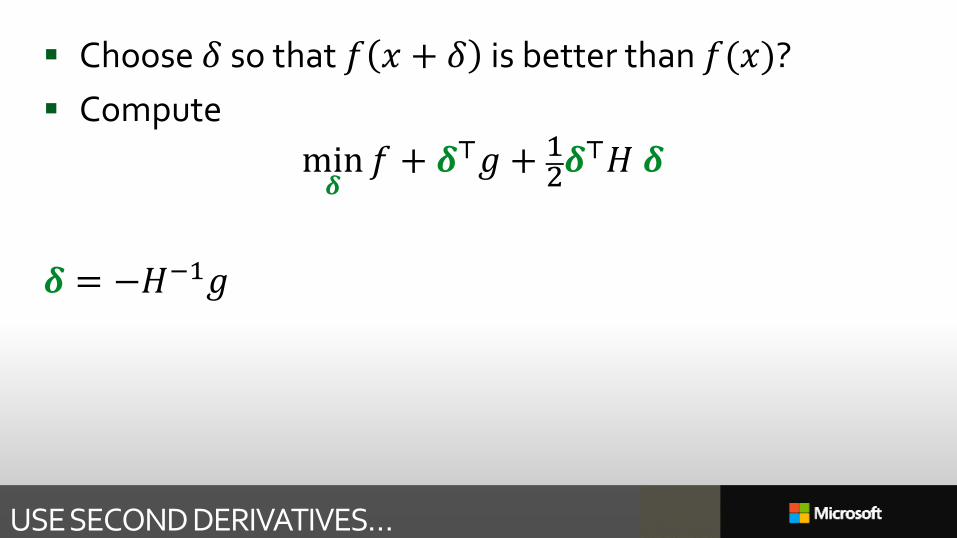
Choose 𝛿 so that 𝑓 𝑥 + 𝛿 is better than 𝑓(𝑥)?

Compute

min𝜹

𝑓 + 𝜹⊤𝑔 + 12𝜹

⊤𝐻 𝜹

𝜹 = −𝐻−1𝑔

IS THAT A GOOD IDEA?

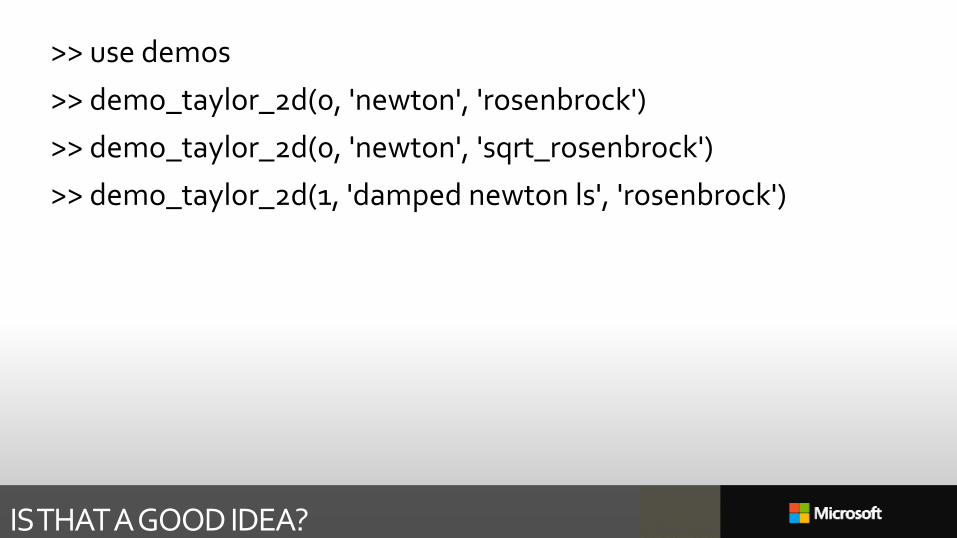
>> use demos

>> demo_taylor_2d(0, 'newton', 'rosenbrock')

>> demo_taylor_2d(0, 'newton', 'sqrt_rosenbrock')

>> demo_taylor_2d(1, 'damped newton ls', 'rosenbrock')

USE SECOND DERIVATIVES…

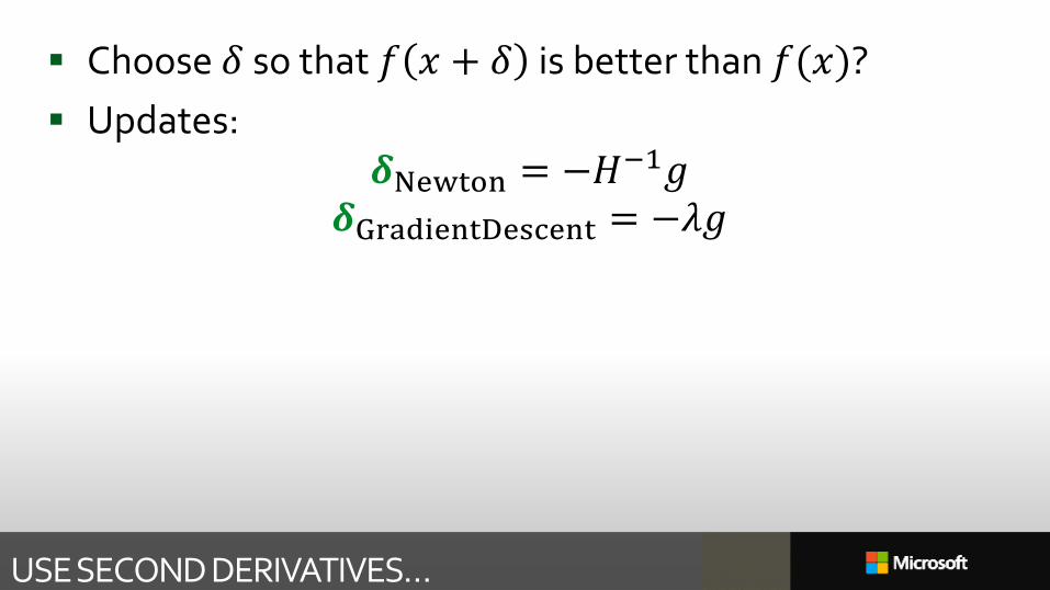
Choose 𝛿 so that 𝑓 𝑥 + 𝛿 is better than 𝑓(𝑥)?

Updates:𝜹Newton = −𝐻−1𝑔

𝜹GradientDescent = −𝜆𝑔

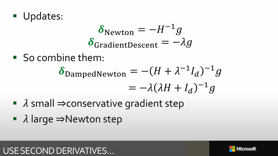
USE SECOND DERIVATIVES…

Updates:𝜹Newton = −𝐻−1𝑔

𝜹GradientDescent = −𝜆𝑔

So combine them:𝜹DampedNewton = − 𝐻 + 𝜆−1𝐼𝑑

−1𝑔

= −𝜆 𝜆𝐻 + 𝐼𝑑−1𝑔

𝜆 small ⇒conservative gradient step

𝜆 large ⇒Newton step

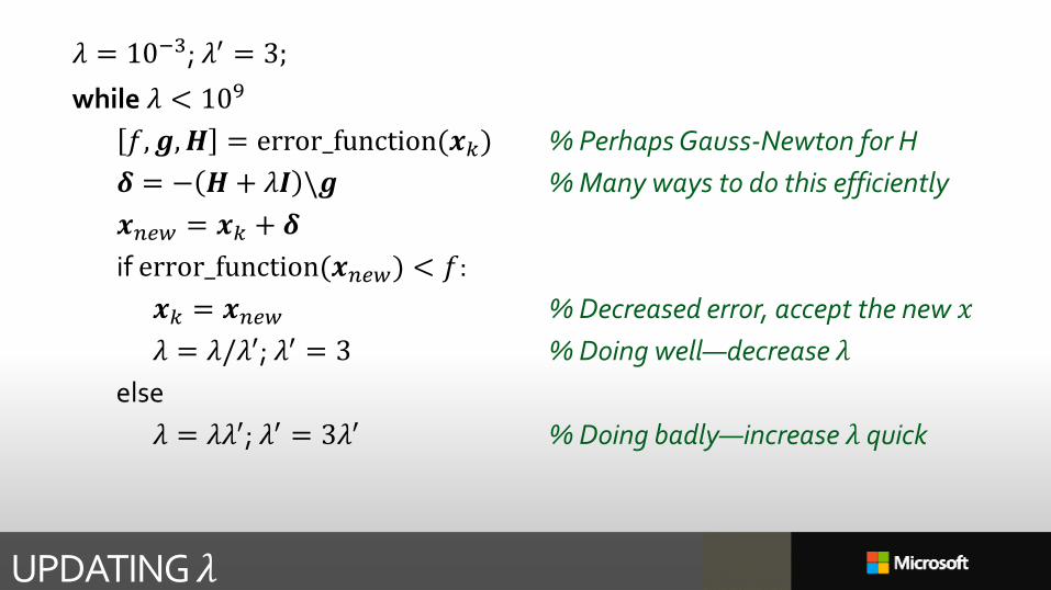
UPDATING 𝜆

𝜆 = 10−3; 𝜆′ = 3;

while 𝜆 < 109

𝑓, 𝒈,𝑯 = error_function(𝒙𝑘) % Perhaps Gauss-Newton for H

𝜹 = − 𝑯+ 𝜆𝑰 \𝒈 % Many ways to do this efficiently

𝒙𝑛𝑒𝑤 = 𝒙𝑘 + 𝜹

if error_function(𝒙𝑛𝑒𝑤) < 𝑓:

𝒙𝑘 = 𝒙𝑛𝑒𝑤 % Decreased error, accept the new 𝑥

𝜆 = 𝜆/𝜆′; 𝜆′ = 3 % Doing well—decrease 𝜆

else

𝜆 = 𝜆𝜆′; 𝜆′ = 3𝜆′ % Doing badly—increase 𝜆 quick

1ST DERIVATIVES AGAIN

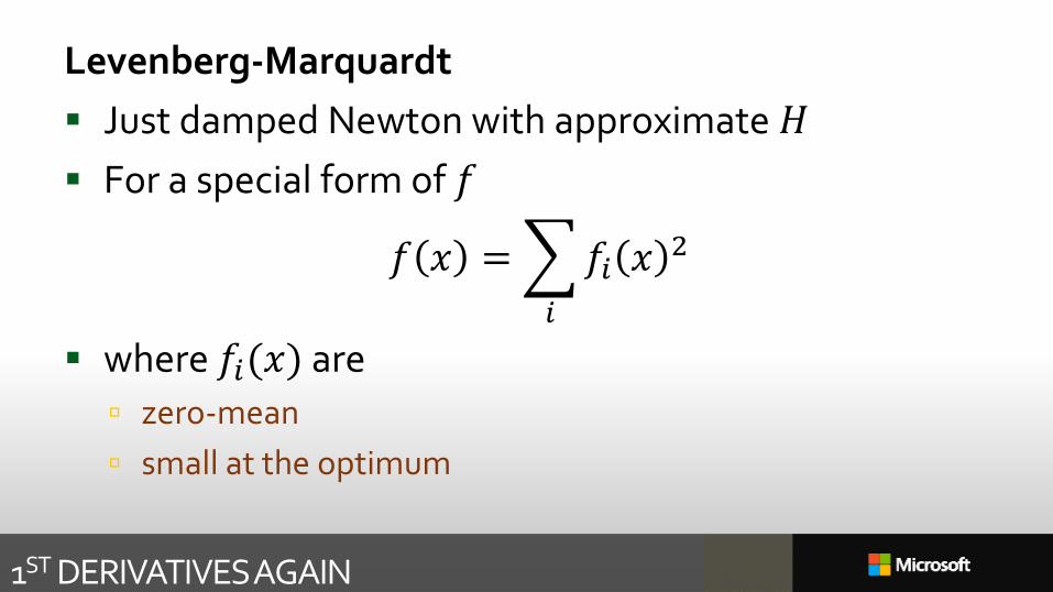
Levenberg-Marquardt

Just damped Newton with approximate 𝐻

For a special form of 𝑓

𝑓 𝑥 =

𝑖

𝑓𝑖 𝑥2

where 𝑓𝑖(𝑥) are

zero-mean

small at the optimum

BACK TO FIRST DERIVATIVES

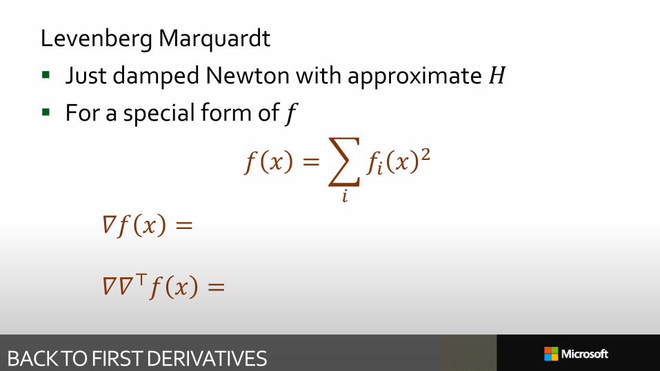
Levenberg Marquardt

Just damped Newton with approximate 𝐻

For a special form of 𝑓

𝑓 𝑥 =

𝑖

𝑓𝑖 𝑥2

𝛻𝑓 𝑥 =

𝛻𝛻⊤𝑓 𝑥 =

BACK TO FIRST DERIVATIVES

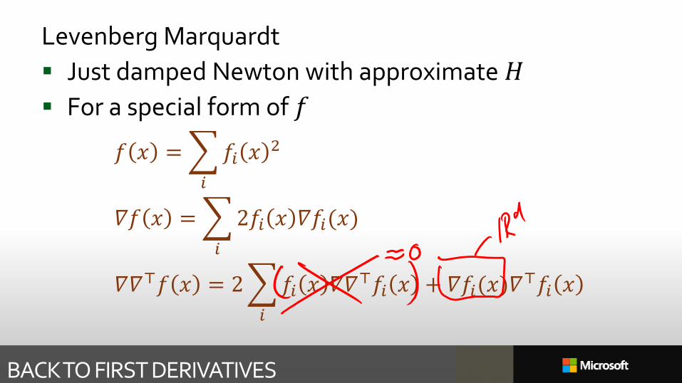
Levenberg Marquardt

Just damped Newton with approximate 𝐻

For a special form of 𝑓

𝑓 𝑥 =

𝑖

𝑓𝑖 𝑥2

𝛻𝑓 𝑥 =

𝑖

2𝑓𝑖 𝑥 𝛻𝑓𝑖(𝑥)

𝛻𝛻⊤𝑓 𝑥 = 2

𝑖

𝑓𝑖 𝑥 𝛻𝛻⊤𝑓𝑖 𝑥 + 𝛻𝑓𝑖(𝑥)𝛻⊤𝑓𝑖 𝑥

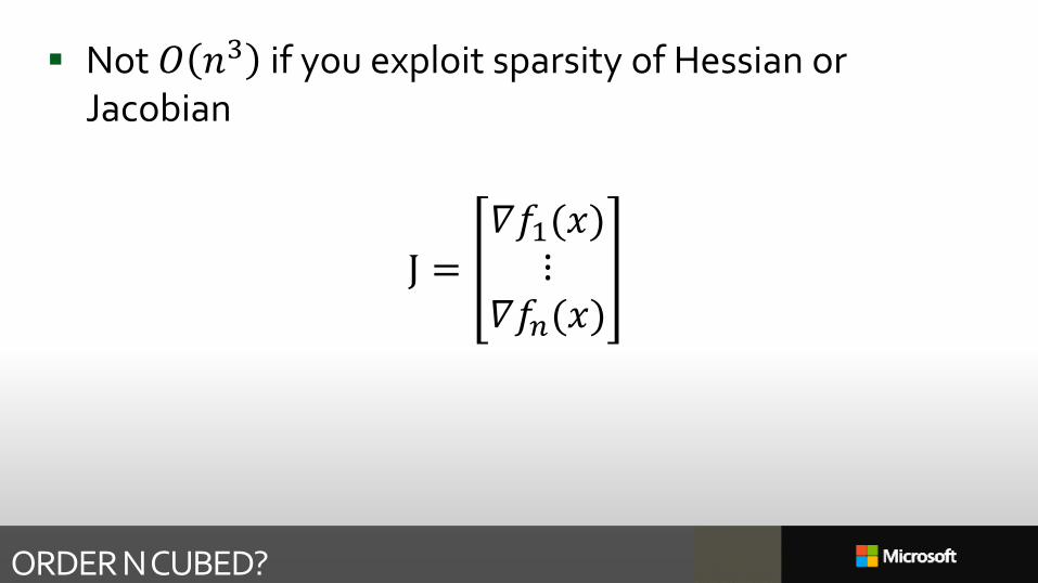
ORDER N CUBED?

Not 𝑂 𝑛3 if you exploit sparsity of Hessian or Jacobian

J =𝛻𝑓1(𝑥)

⋮𝛻𝑓𝑛(𝑥)

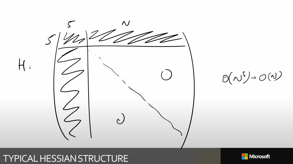
TYPICAL HESSIAN STRUCTURE

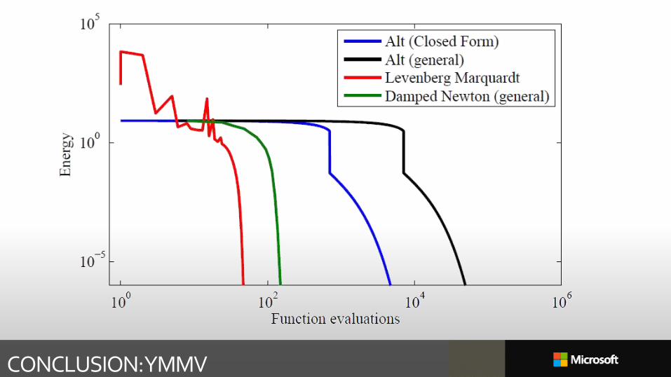
CONCLUSION: YMMV

CONCLUSION: YMMV

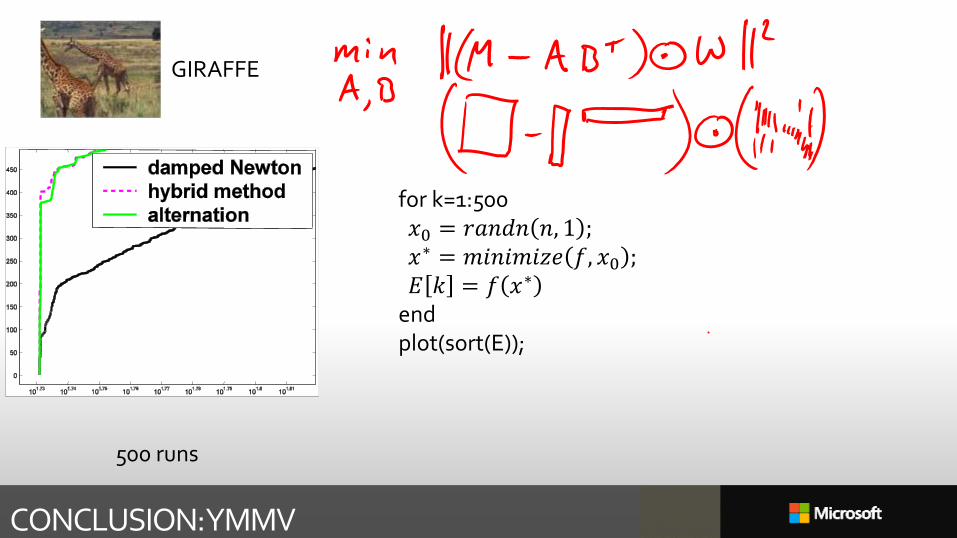
GIRAFFE

500 runs

for k=1:500𝑥0 = 𝑟𝑎𝑛𝑑𝑛 𝑛, 1 ;𝑥∗ = 𝑚𝑖𝑛𝑖𝑚𝑖𝑧𝑒 𝑓, 𝑥0 ;𝐸 𝑘 = 𝑓 𝑥∗

endplot(sort(E));

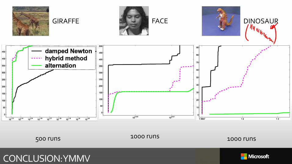
CONCLUSION: YMMV

FACE

1000 runs

DINOSAUR

1000 runs

GIRAFFE

500 runs

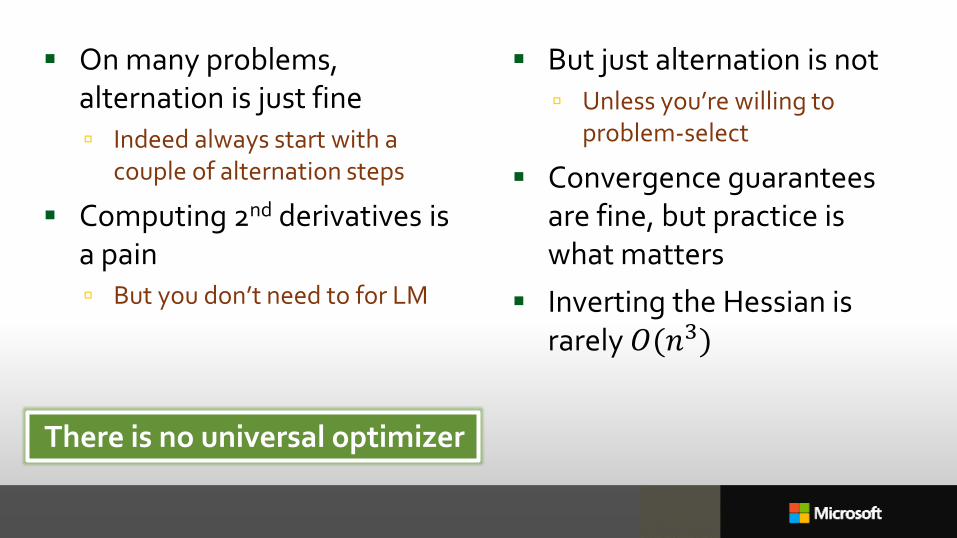
On many problems, alternation is just fine Indeed always start with a

couple of alternation steps

Computing 2nd derivatives is a pain But you don’t need to for LM

But just alternation is not Unless you’re willing to

problem-select

Convergence guarantees are fine, but practice is what matters

Inverting the Hessian is rarely 𝑂(𝑛3)

There is no universal optimizer

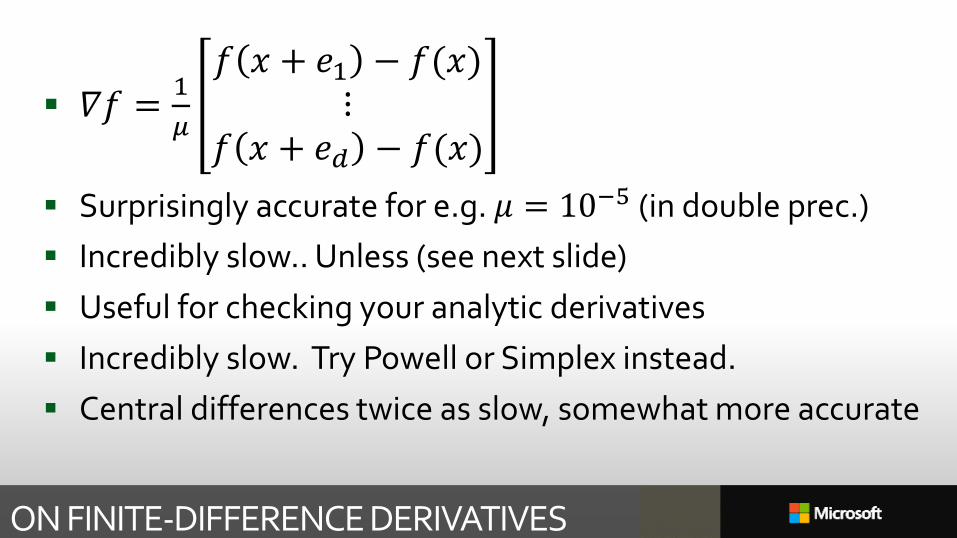
ON FINITE-DIFFERENCE DERIVATIVES

𝛻𝑓 =1

𝜇

𝑓 𝑥 + 𝑒1 − 𝑓(𝑥)⋮

𝑓 𝑥 + 𝑒𝑑 − 𝑓(𝑥)

Surprisingly accurate for e.g. 𝜇 = 10−5 (in double prec.)

Incredibly slow.. Unless (see next slide)

Useful for checking your analytic derivatives

Incredibly slow. Try Powell or Simplex instead.

Central differences twice as slow, somewhat more accurate

GRAPH COLOURING FOR FINITE DIFFS

Normally try 𝑒1 to 𝑒𝑑 sequentially

But if we know the nonzero structure of the Jacobian, can go rather faster.

134

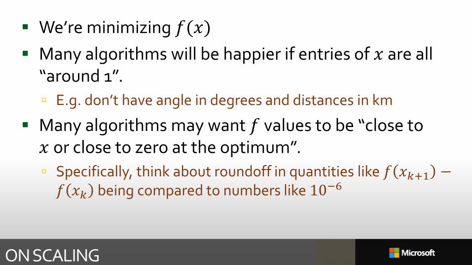
ON SCALING

We’re minimizing 𝑓(𝑥)

Many algorithms will be happier if entries of 𝑥 are all “around 1”.

E.g. don’t have angle in degrees and distances in km

Many algorithms may want 𝑓 values to be “close to 𝑥 or close to zero at the optimum”.

Specifically, think about roundoff in quantities like 𝑓 𝑥𝑘+1 −𝑓 𝑥𝑘 being compared to numbers like 10−6

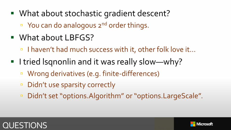
QUESTIONS

What about stochastic gradient descent?

You can do analogous 2nd order things.

What about LBFGS?

I haven’t had much success with it, other folk love it…

I tried lsqnonlin and it was really slow—why?

Wrong derivatives (e.g. finite-differences)

Didn’t use sparsity correctly

Didn’t set “options.Algorithm” or “options.LargeScale”.

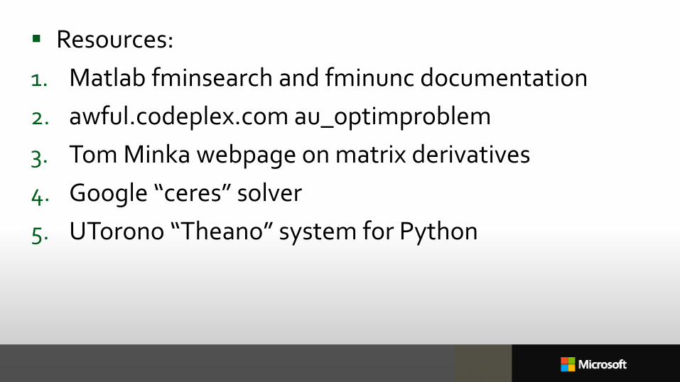
Resources:

1. Matlab fminsearch and fminunc documentation

2. awful.codeplex.com au_optimproblem

3. Tom Minka webpage on matrix derivatives

4. Google “ceres” solver

5. UTorono “Theano” system for Python

Gotchas with lsqnonlin opts.LargeScale = 'on';

opts.Jacobian = 'on';

Need non-rank-def J?

Need to implement JacobMult?

WHAT IS A SURFACE?

143

0 0.2 0.4 0.6 0.8 11.92

2.12.22.32.4

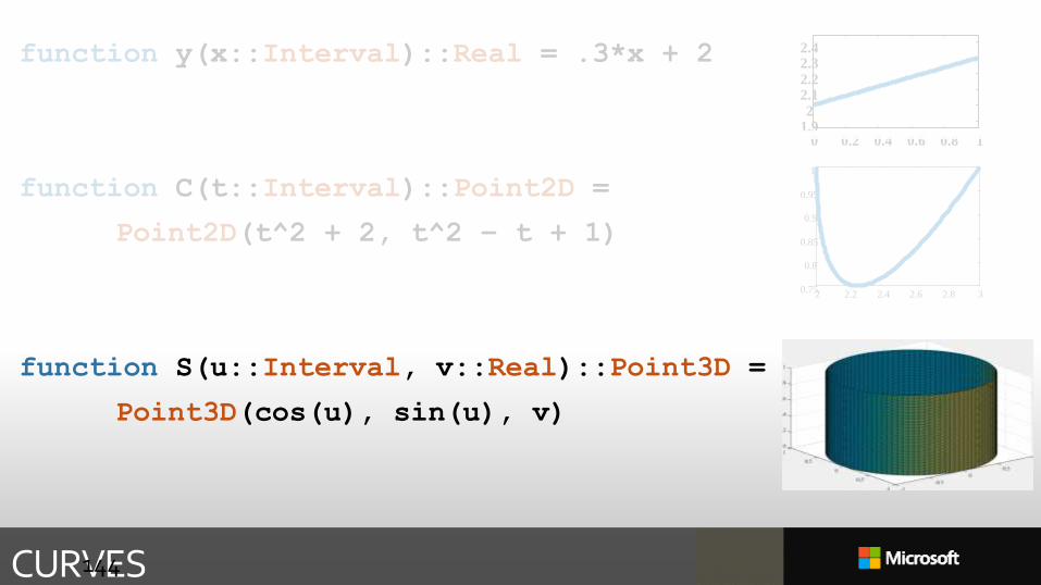
CURVES

function y(x::Interval)::Real = .3*x + 2

function C(t::Interval)::Point2D =

Point2D(t^2 + 2, t^2 – t + 1)

function S(u::Interval, v::Real)::Point3D =

Point3D(cos(u), sin(u), v)

144

2 2.2 2.4 2.6 2.8 30.75

0.8

0.85

0.9

0.95

1

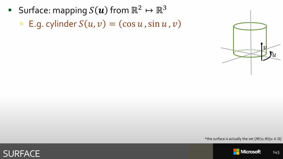
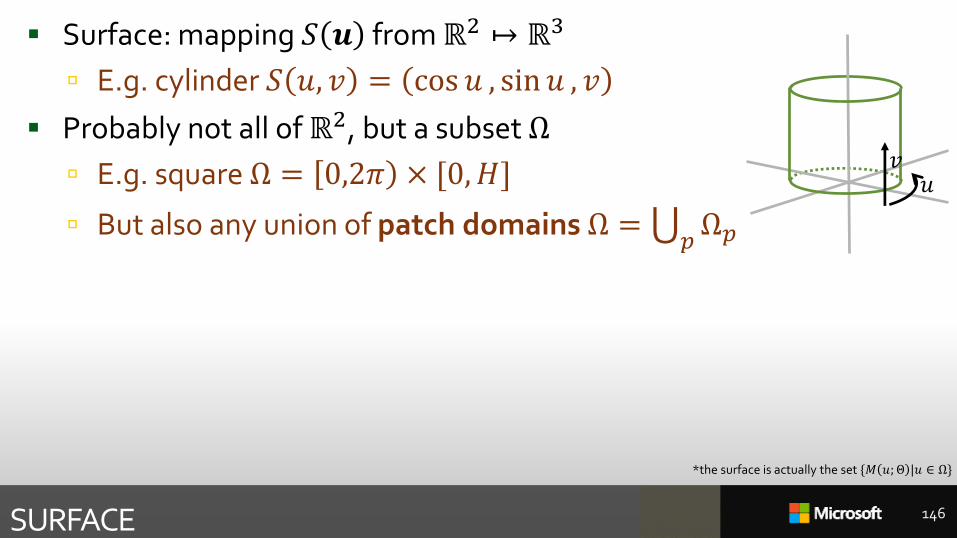
Surface: mapping 𝑆 𝒖 from ℝ2 ↦ ℝ3

E.g. cylinder 𝑆 𝑢, 𝑣 = cos 𝑢 , sin 𝑢 , 𝑣

SURFACE 145

*the surface is actually the set {𝑀 𝑢; Θ |𝑢 ∈ Ω}

𝑢𝑣

Surface: mapping 𝑆 𝒖 from ℝ2 ↦ ℝ3

E.g. cylinder 𝑆 𝑢, 𝑣 = cos 𝑢 , sin 𝑢 , 𝑣

Probably not all of ℝ2, but a subset Ω

E.g. square Ω = 0,2𝜋 × [0,𝐻]

But also any union of patch domains Ω = ሪ𝑝Ω𝑝

SURFACE 146

*the surface is actually the set {𝑀 𝑢; Θ |𝑢 ∈ Ω}

𝑢𝑣

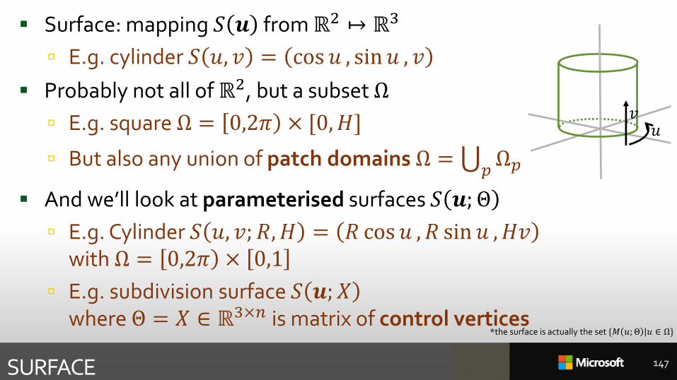
Surface: mapping 𝑆 𝒖 from ℝ2 ↦ ℝ3

E.g. cylinder 𝑆 𝑢, 𝑣 = cos 𝑢 , sin 𝑢 , 𝑣

Probably not all of ℝ2, but a subset Ω

E.g. square Ω = 0,2𝜋 × [0,𝐻]

But also any union of patch domains Ω = ሪ𝑝Ω𝑝

And we’ll look at parameterised surfaces 𝑆 𝒖; Θ

E.g. Cylinder 𝑆 𝑢, 𝑣; 𝑅, 𝐻 = 𝑅 cos 𝑢 , 𝑅 sin 𝑢 , 𝐻𝑣with Ω = 0,2𝜋 × 0,1

E.g. subdivision surface 𝑆 𝒖; 𝑋where Θ = 𝑋 ∈ ℝ3×𝑛 is matrix of control vertices

SURFACE 147

*the surface is actually the set {𝑀 𝑢; Θ |𝑢 ∈ Ω}

𝑢𝑣

TOOL: SUBDIVISION SURFACES

148

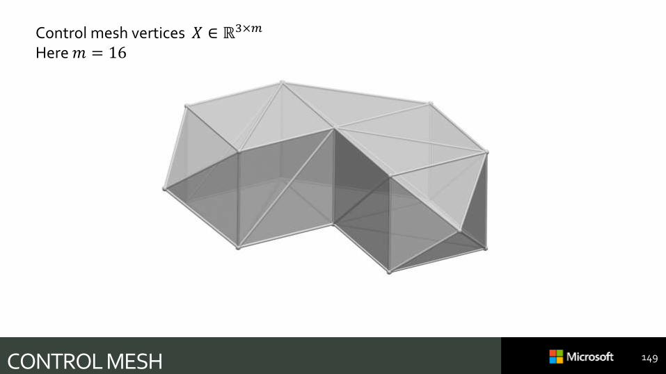
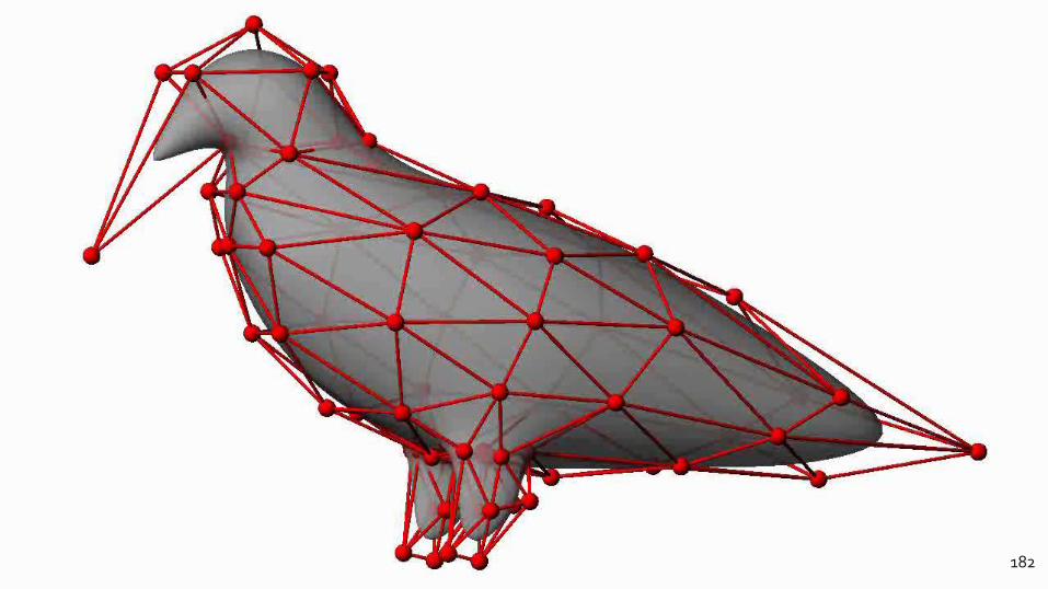
CONTROL MESH 149

Control mesh vertices 𝑋 ∈ ℝ3×𝑚

Here 𝑚 = 16

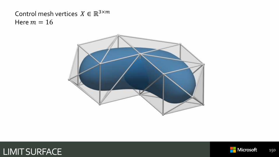
LIMIT SURFACE 150

Control mesh vertices 𝑋 ∈ ℝ3×𝑚

Here 𝑚 = 16

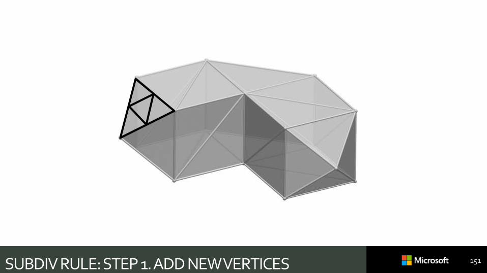
SUBDIV RULE: STEP 1. ADD NEW VERTICES 151

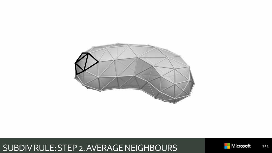
SUBDIV RULE: STEP 2. AVERAGE NEIGHBOURS 152

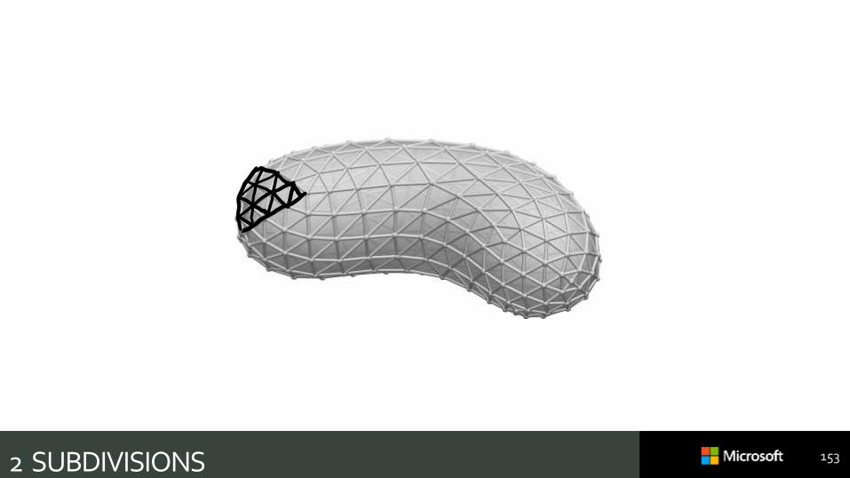
2 SUBDIVISIONS 153

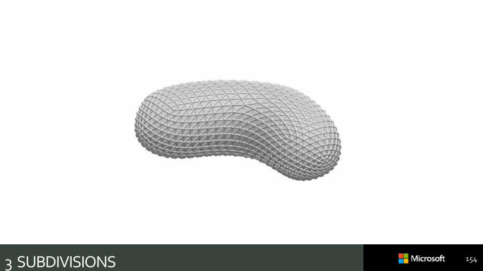
3 SUBDIVISIONS 154

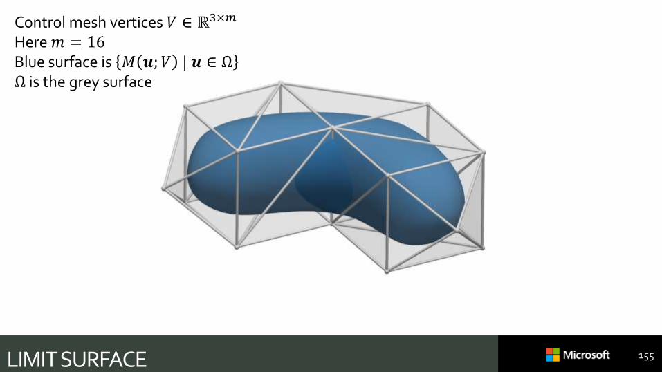
LIMIT SURFACE 155

Control mesh vertices 𝑉 ∈ ℝ3×𝑚

Here 𝑚 = 16Blue surface is 𝑀 𝒖;𝑉 | 𝒖 ∈ ΩΩ is the grey surface

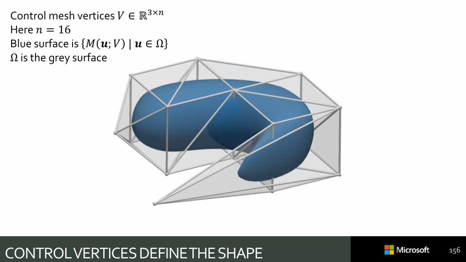
CONTROL VERTICES DEFINE THE SHAPE 156

Control mesh vertices 𝑉 ∈ ℝ3×𝑛

Here 𝑛 = 16Blue surface is 𝑀 𝒖;𝑉 | 𝒖 ∈ ΩΩ is the grey surface

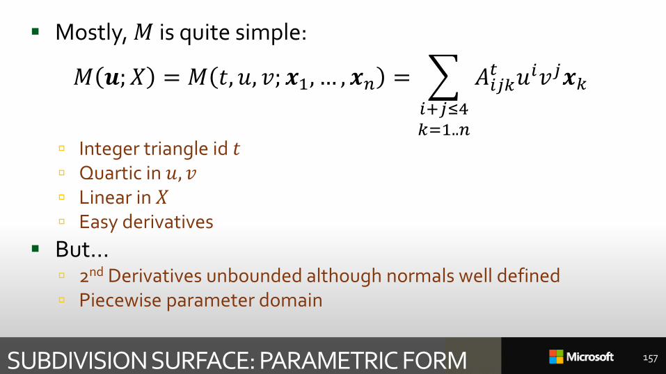
Mostly, 𝑀 is quite simple:

𝑀 𝒖;𝑋 = 𝑀 𝑡, 𝑢, 𝑣; 𝒙1, … , 𝒙𝑛 = 𝑖+𝑗≤4𝑘=1..𝑛

𝐴𝑖𝑗𝑘𝑡 𝑢𝑖𝑣𝑗𝒙𝑘

Integer triangle id 𝑡 Quartic in 𝑢, 𝑣 Linear in 𝑋 Easy derivatives

But… 2nd Derivatives unbounded although normals well defined Piecewise parameter domain

SUBDIVISION SURFACE: PARAMETRIC FORM 157

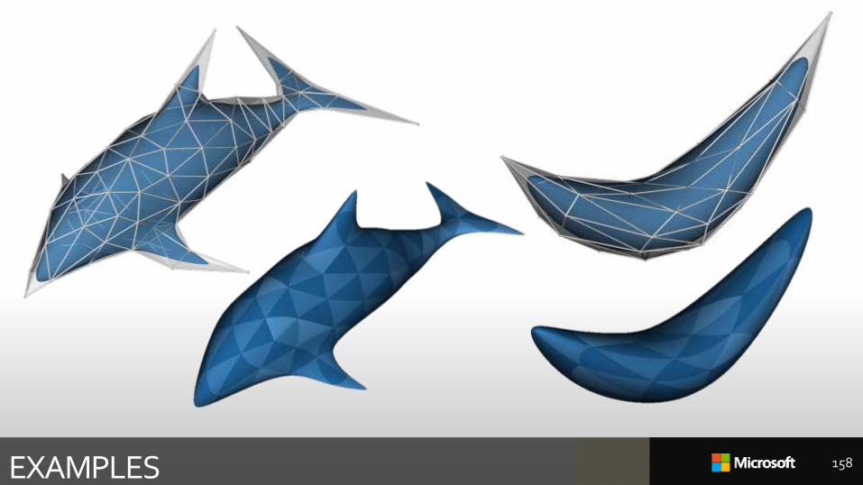
EXAMPLES 158

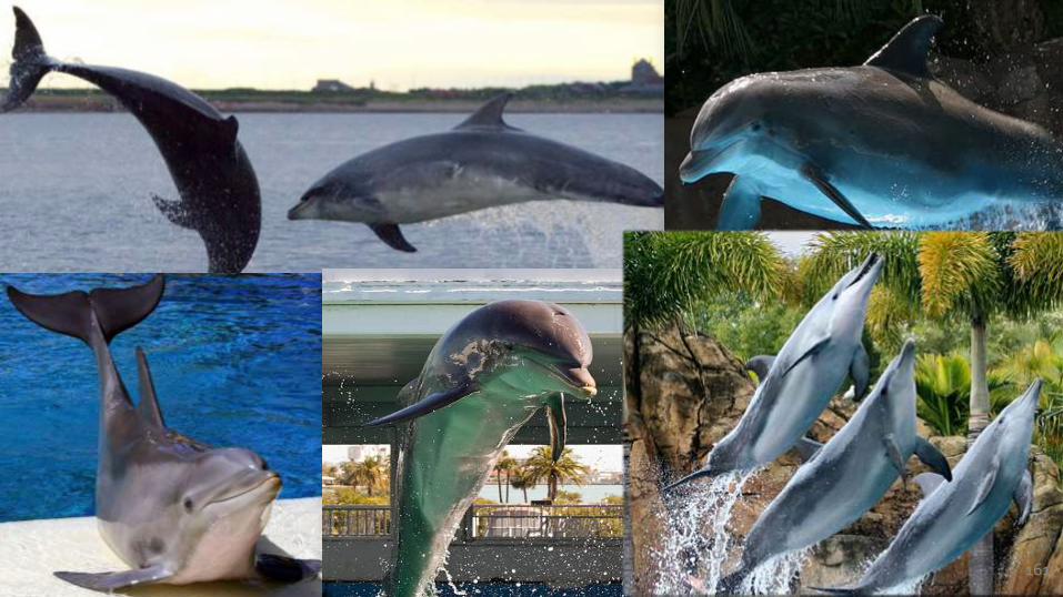
BACK TO DOLPHINS

159

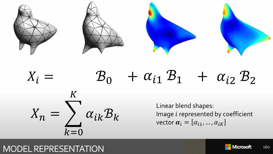
MODEL REPRESENTATION

𝑋𝑛 =

𝑘=0

𝐾

𝛼𝑖𝑘ℬ𝑘

𝛼𝑖1 ℬ1 𝛼𝑖2 ℬ2+ +𝑋𝑖 =

Linear blend shapes: Image 𝑖 represented by coefficient vector 𝜶𝑖 = 𝛼𝑖1, … , 𝛼𝑖𝐾

ℬ0

160

161

162

164

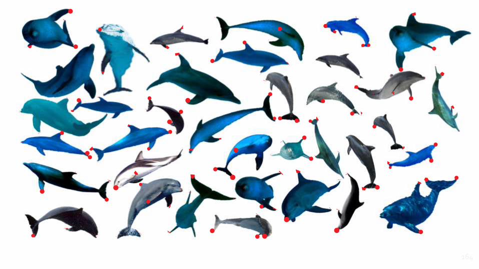
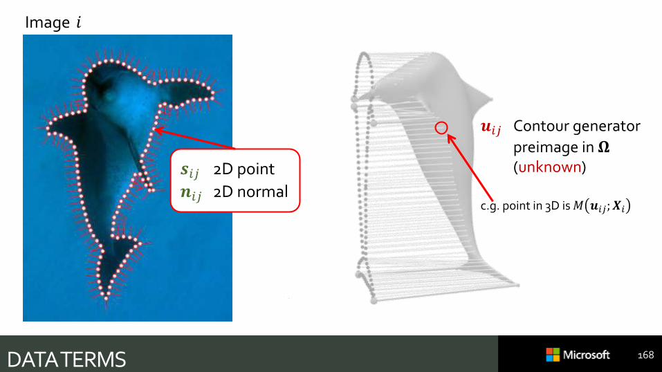
𝒔𝑖𝑗 2D point

𝒏𝑖𝑗 2D normal

DATA TERMS

Image 𝑖

𝒖𝑖𝑗 Contour generator

preimage in 𝛀(unknown)

c.g. point in 3D is 𝑀 𝒖𝑖𝑗; 𝑿𝑖

167

𝒔𝑖𝑗 2D point

𝒏𝑖𝑗 2D normal

DATA TERMS

Image 𝑖

𝒖𝑖𝑗 Contour generator

preimage in 𝛀(unknown)

c.g. point in 3D is 𝑀 𝒖𝑖𝑗; 𝑿𝑖

168

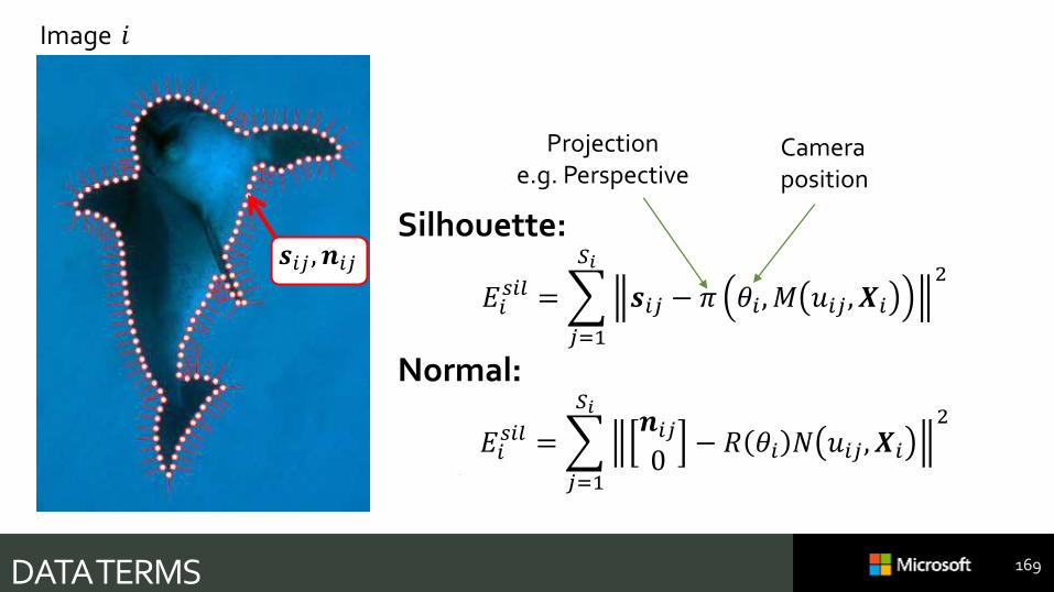
DATA TERMS

Image 𝑖

𝒔𝑖𝑗 , 𝒏𝑖𝑗

169

Camera position

Silhouette:

𝐸𝑖𝑠𝑖𝑙 =

𝑗=1

𝑆𝑖

𝒔𝑖𝑗 − 𝜋 𝜃𝑖 , 𝑀 𝑢𝑖𝑗 , 𝑿𝑖

2

Normal:

𝐸𝑖𝑠𝑖𝑙 =

𝑗=1

𝑆𝑖𝒏𝑖𝑗0

− 𝑅 𝜃𝑖 𝑁 𝑢𝑖𝑗 , 𝑿𝑖

2

Projectione.g. Perspective

DATA TERMS

Image 𝑖

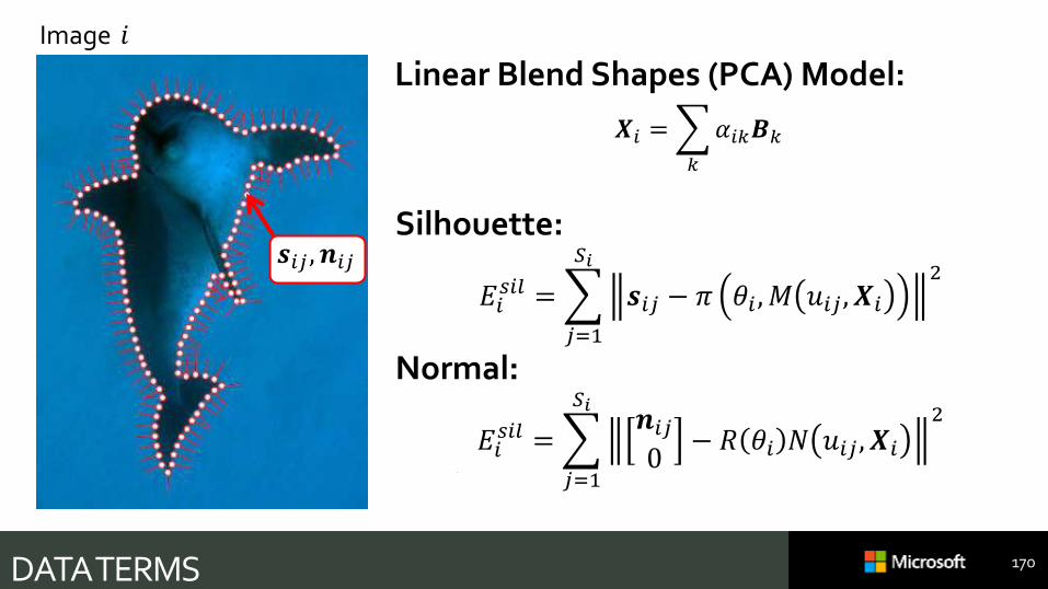
𝒔𝑖𝑗 , 𝒏𝑖𝑗

Linear Blend Shapes (PCA) Model:

𝑿𝑖 =

𝑘

𝛼𝑖𝑘𝑩𝑘

170

Silhouette:

𝐸𝑖𝑠𝑖𝑙 =

𝑗=1

𝑆𝑖

𝒔𝑖𝑗 − 𝜋 𝜃𝑖 , 𝑀 𝑢𝑖𝑗 , 𝑿𝑖

2

Normal:

𝐸𝑖𝑠𝑖𝑙 =

𝑗=1

𝑆𝑖𝒏𝑖𝑗0

− 𝑅 𝜃𝑖 𝑁 𝑢𝑖𝑗 , 𝑿𝑖

2

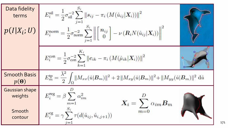
Data fidelity terms

𝑝 𝐼 𝑋𝑖; 𝑈

Gaussian shape weights

Smooth contour

Smooth Basis𝑝 𝚯

171

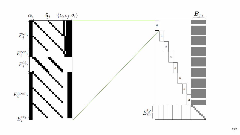
172

CONTINOUSOPTIMIZATION

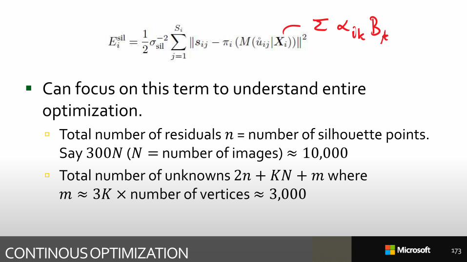
Can focus on this term to understand entire optimization.

Total number of residuals 𝑛 = number of silhouette points. Say 300𝑁 (𝑁 = number of images) ≈ 10,000

Total number of unknowns 2𝑛 + 𝐾𝑁 +𝑚 where 𝑚 ≈ 3𝐾 × number of vertices ≈ 3,000

173

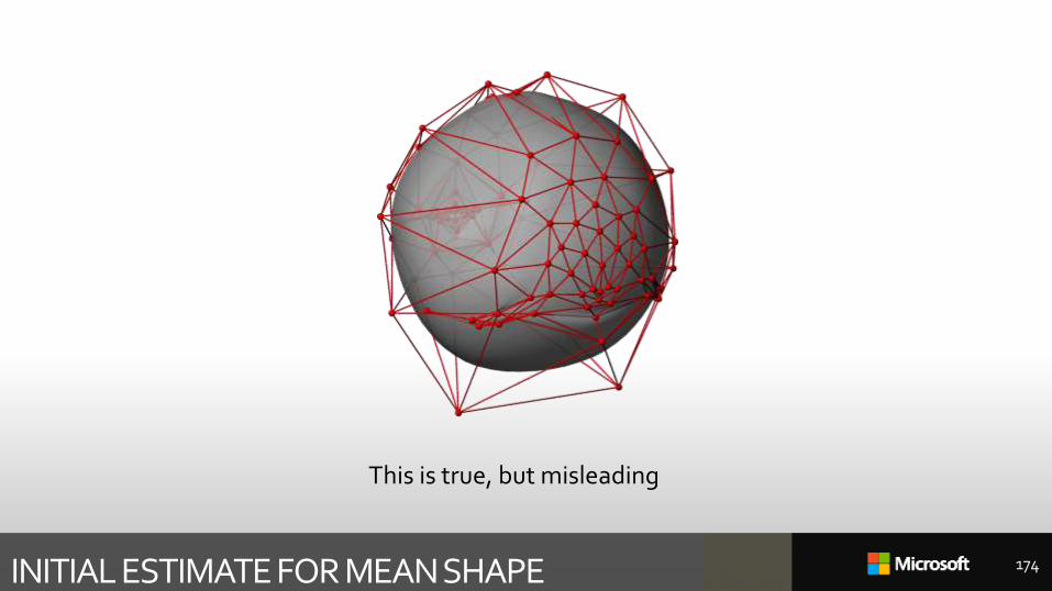
INITIAL ESTIMATE FOR MEAN SHAPE

This is true, but misleading

174

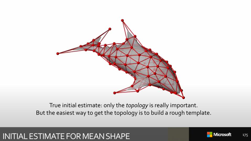
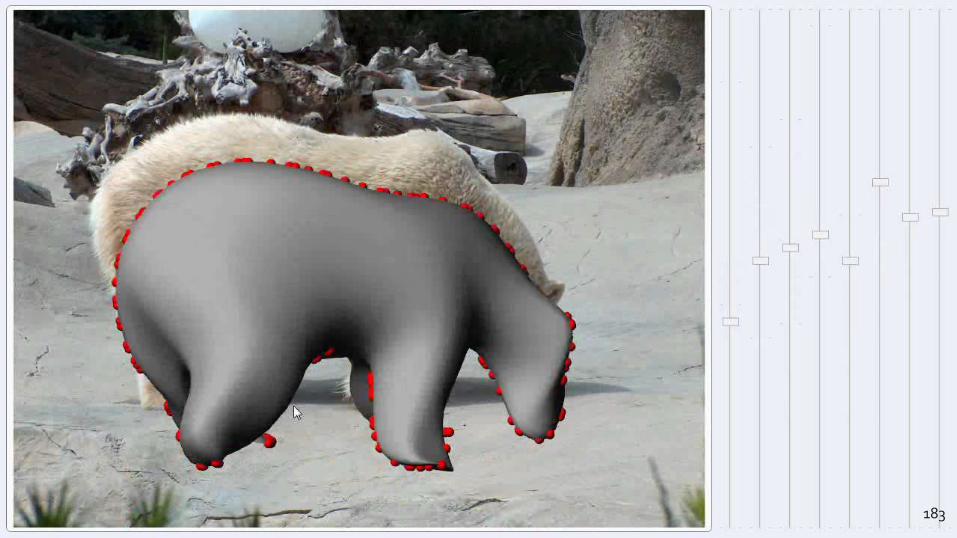
INITIAL ESTIMATE FOR MEAN SHAPE

True initial estimate: only the topology is really important.But the easiest way to get the topology is to build a rough template.

175

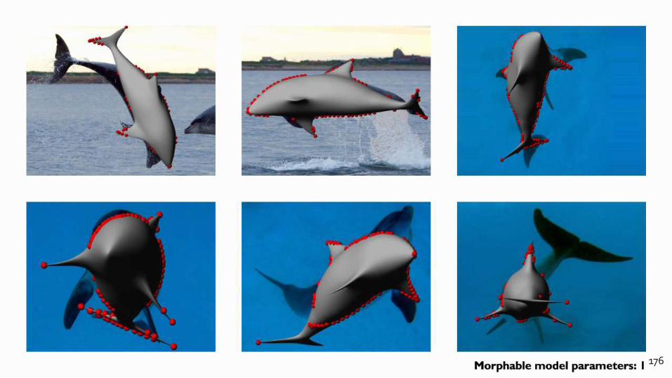
176

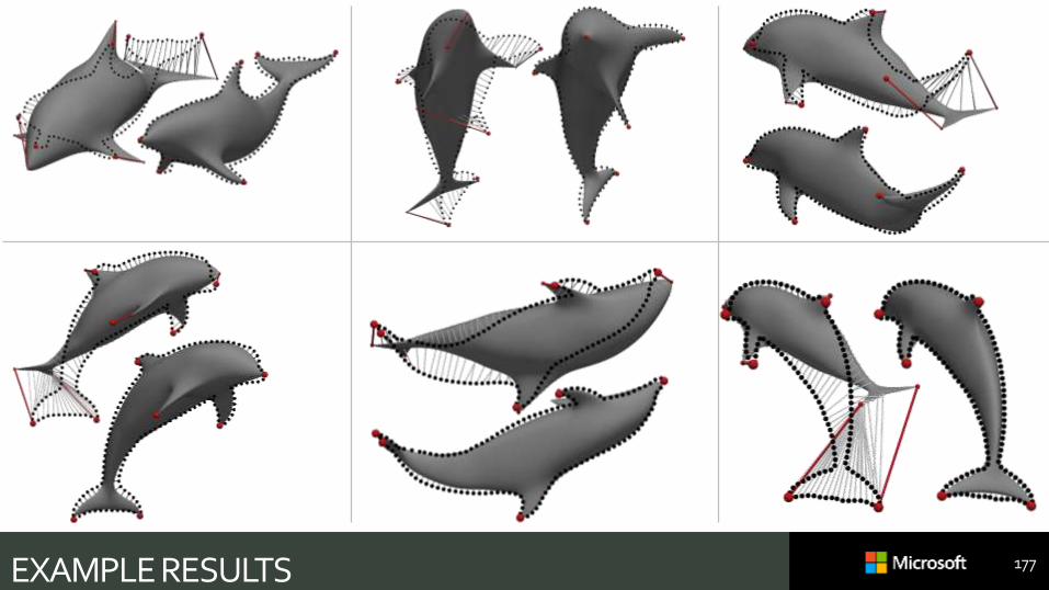
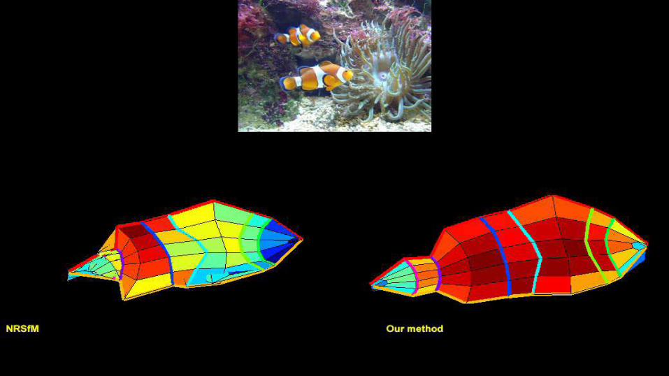
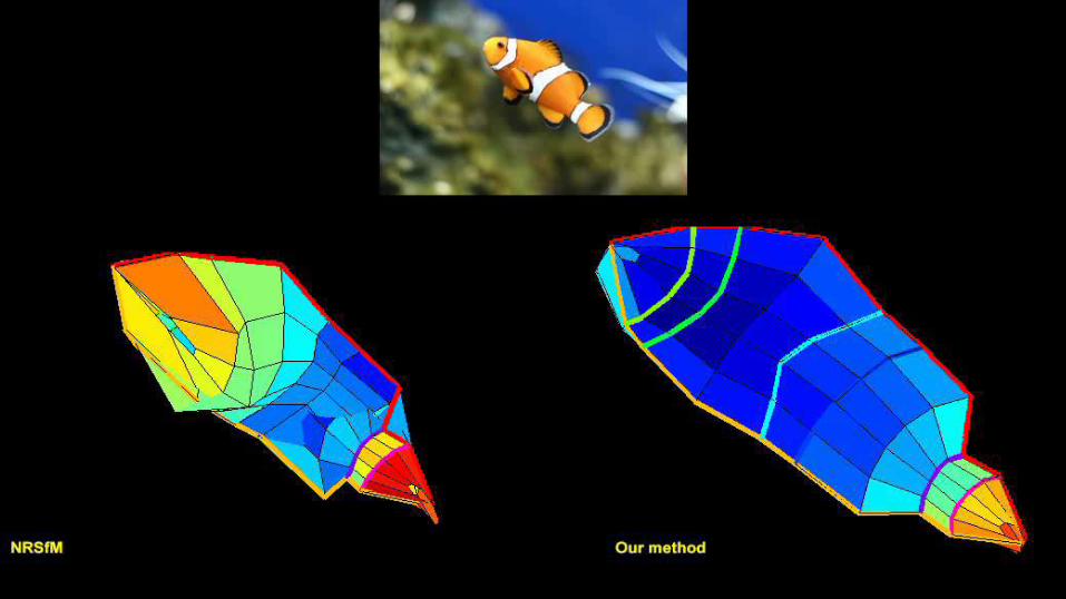
EXAMPLE RESULTS 177

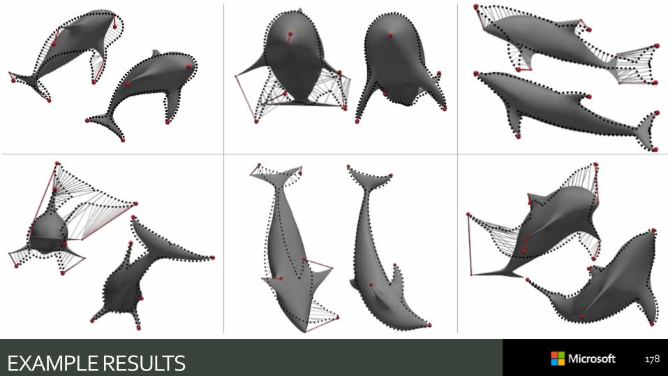
EXAMPLE RESULTS 178

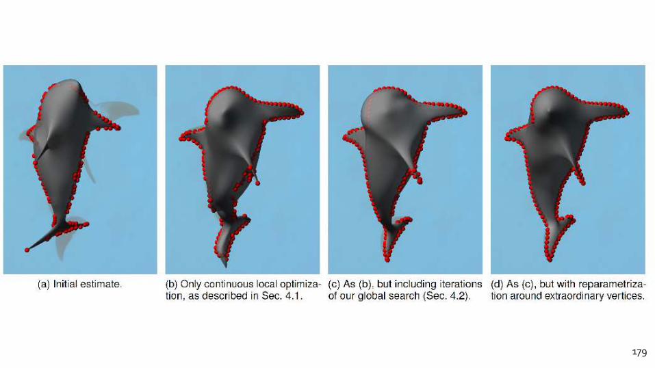
OPTIMIZATION 179

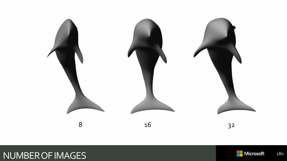
NUMBER OF IMAGES 180

8 16 32

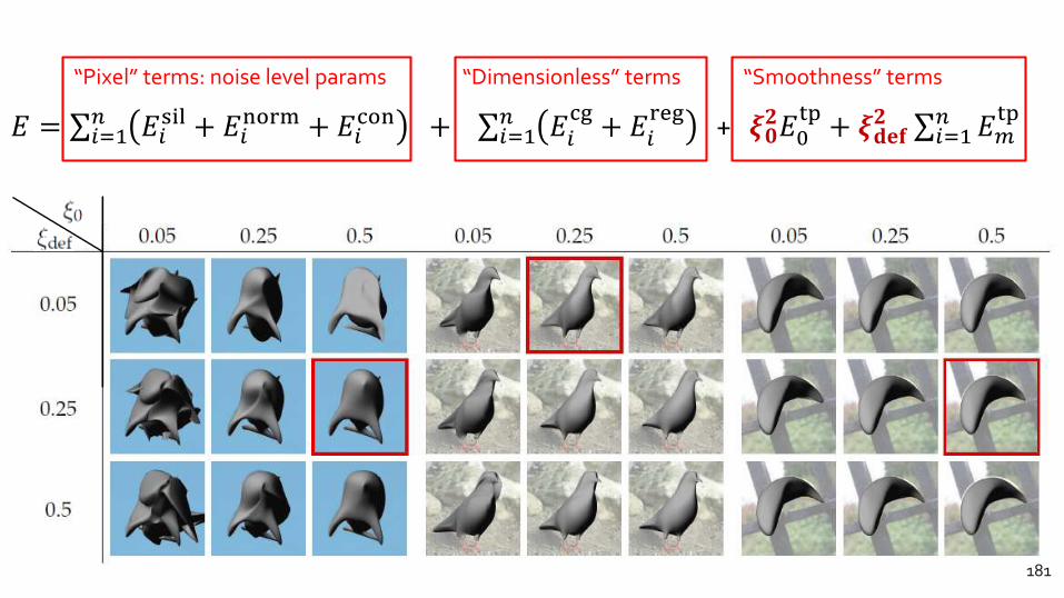
PARAMETER SENSITIVITY“Pixel” terms: noise level params “Dimensionless” terms “Smoothness” terms

𝐸 = σ𝑖=1𝑛 𝐸𝑖

sil + 𝐸𝑖norm + 𝐸𝑖

con + σ𝑖=1𝑛 𝐸𝑖

cg+ 𝐸𝑖

reg+ 𝝃𝟎

𝟐𝐸0tp+ 𝝃𝐝𝐞𝐟

𝟐 σ𝑖=1𝑛 𝐸𝑚

tp

181

182

183

184

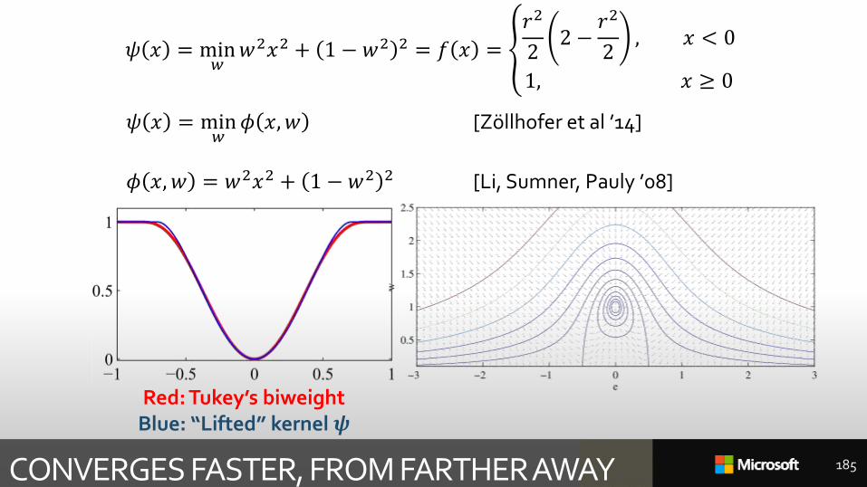
CONVERGES FASTER, FROM FARTHER AWAY 185

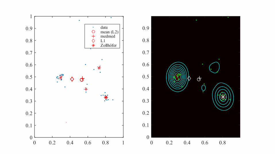
𝜓 𝑥 = min𝑤

𝜙 𝑥,𝑤 [Zöllhofer et al ’14]

𝜙 𝑥, 𝑤 = 𝑤2𝑥2 + 1 − 𝑤2 2 [Li, Sumner, Pauly ’08]

Red: Tukey’s biweightBlue: “Lifted” kernel 𝝍

𝜓 𝑥 = min𝑤

𝑤2𝑥2 + 1 − 𝑤2 2 = 𝑓 𝑥 = ൞

𝑟2

22 −

𝑟2

2, 𝑥 < 0

1, 𝑥 ≥ 0

[BLACK AND RANGARANJAN, CVPR 91] – NEARLY[LI, PAULY, SUMNER, SIGGRAPH 08] – NEARLY[ZOLLHÖFER, SIGGRAPH 14] — BASICALLY [ZACH, ECCV 14] — DEFINITELY

Robust estimation

0 0.2 0.4 0.6 0.8 10

0.1

0.2

0.3

0.4

0.5

0.6

0.7

0.8

0.9

1

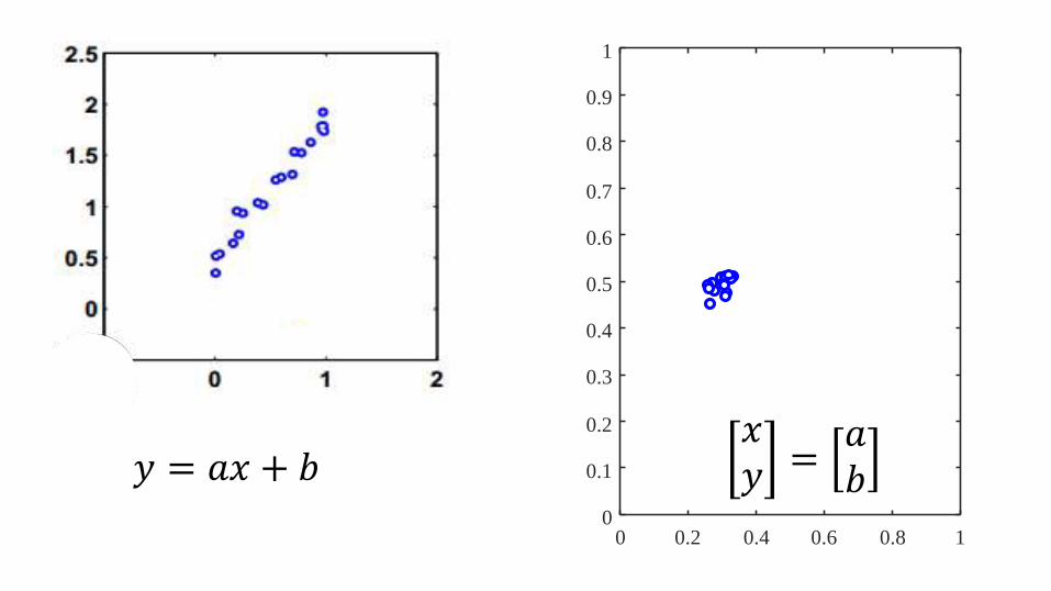
𝑦 = 𝑎𝑥 + 𝑏𝑥𝑦 =

𝑎𝑏

0 0.2 0.4 0.6 0.8 10

0.1

0.2

0.3

0.4

0.5

0.6

0.7

0.8

0.9

1

𝑦 = 𝑎𝑥 + 𝑏𝑥𝑦 =

𝑎𝑏

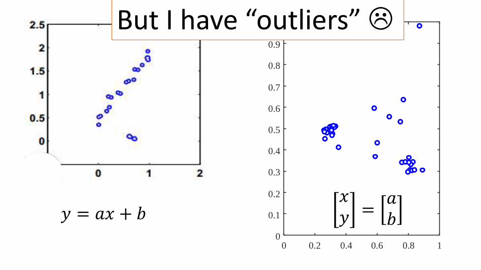
But I have “outliers”

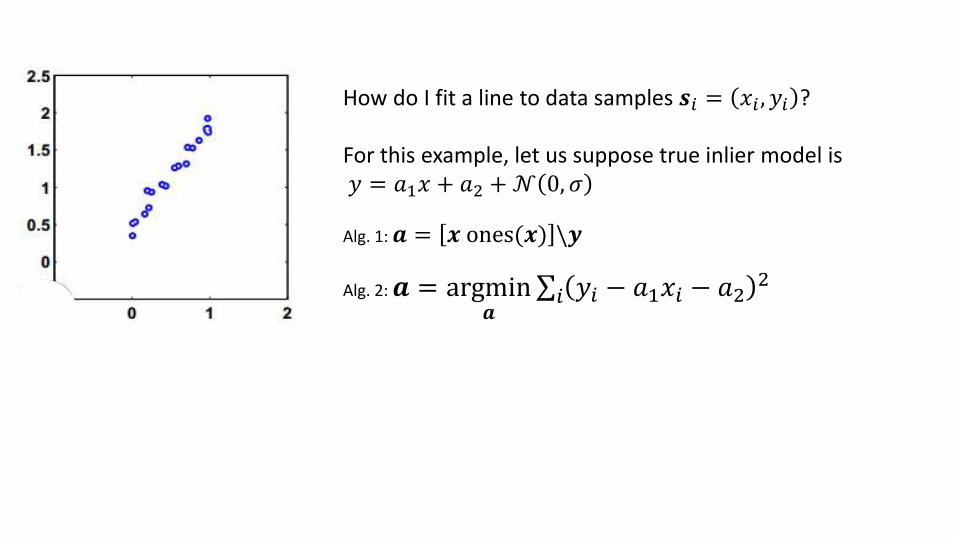
How do I fit a line to data samples 𝒔𝑖 = 𝑥𝑖 , 𝑦𝑖 ?

For this example, let us suppose true inlier model is𝑦 = 𝑎1𝑥 + 𝑎2 +𝒩 0, 𝜎

Alg. 1: 𝒂 = 𝒙 ones(𝒙) \𝒚

Alg. 2: 𝒂 = argmin𝒂

σ𝑖 𝑦𝑖 − 𝑎1𝑥𝑖 − 𝑎22

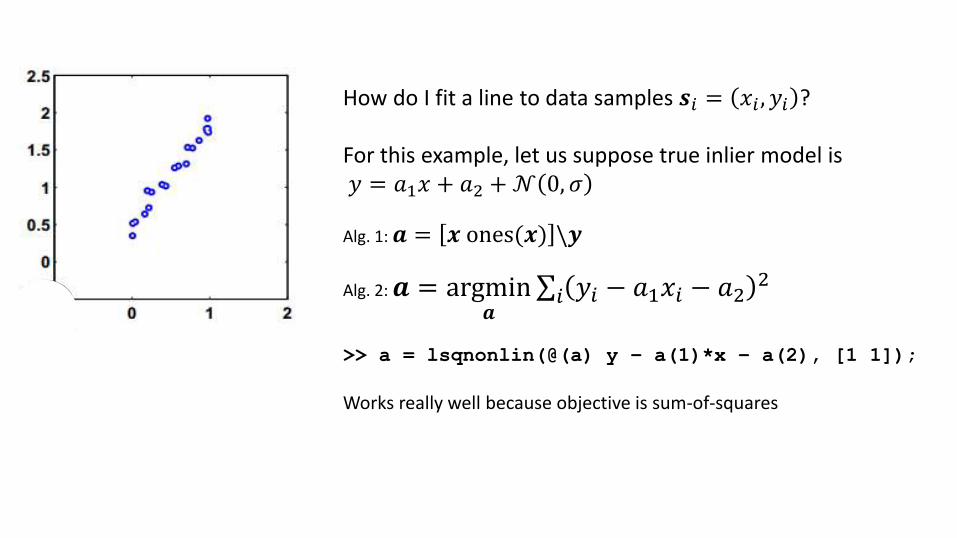
How do I fit a line to data samples 𝒔𝑖 = 𝑥𝑖 , 𝑦𝑖 ?

For this example, let us suppose true inlier model is𝑦 = 𝑎1𝑥 + 𝑎2 +𝒩 0, 𝜎

Alg. 1: 𝒂 = 𝒙 ones(𝒙) \𝒚

Alg. 2: 𝒂 = argmin𝒂

σ𝑖 𝑦𝑖 − 𝑎1𝑥𝑖 − 𝑎22

>> a = lsqnonlin(@(a) y – a(1)*x – a(2), [1 1]);

Works really well because objective is sum-of-squares

How do I fit a line to data samples 𝒔𝑖 = 𝑥𝑖 , 𝑦𝑖 ?

For this example, let us suppose true inlier model is𝑦 = 𝑎𝑥 + 𝑏 +𝒩 0, 𝜎

Alg. 1: 𝒂 = 𝒙 ones(𝒙) \𝒚

Alg. 2: 𝒂 =?

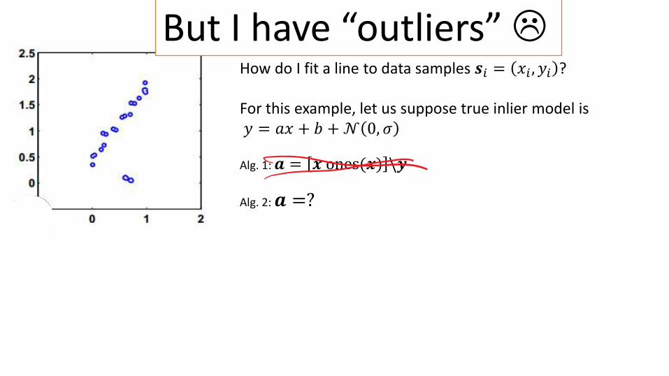
But I have “outliers”

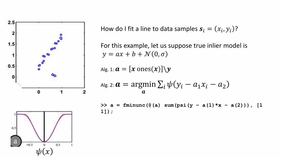
How do I fit a line to data samples 𝒔𝑖 = 𝑥𝑖 , 𝑦𝑖 ?

For this example, let us suppose true inlier model is𝑦 = 𝑎𝑥 + 𝑏 +𝒩 0, 𝜎

Alg. 1: 𝒂 = 𝒙 ones(𝒙) \𝒚

Alg. 2: 𝒂 = argmin𝒂

σ𝑖𝜓 𝑦𝑖 − 𝑎1𝑥𝑖 − 𝑎2

>> a = fminunc(@(a) sum(psi(y – a(1)*x – a(2))), [1

1]);

𝜓 𝑥

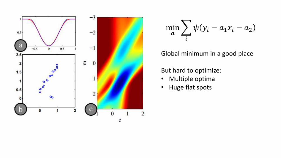
min𝒂

𝑖

𝜓 𝑦𝑖 − 𝑎1𝑥𝑖 − 𝑎2

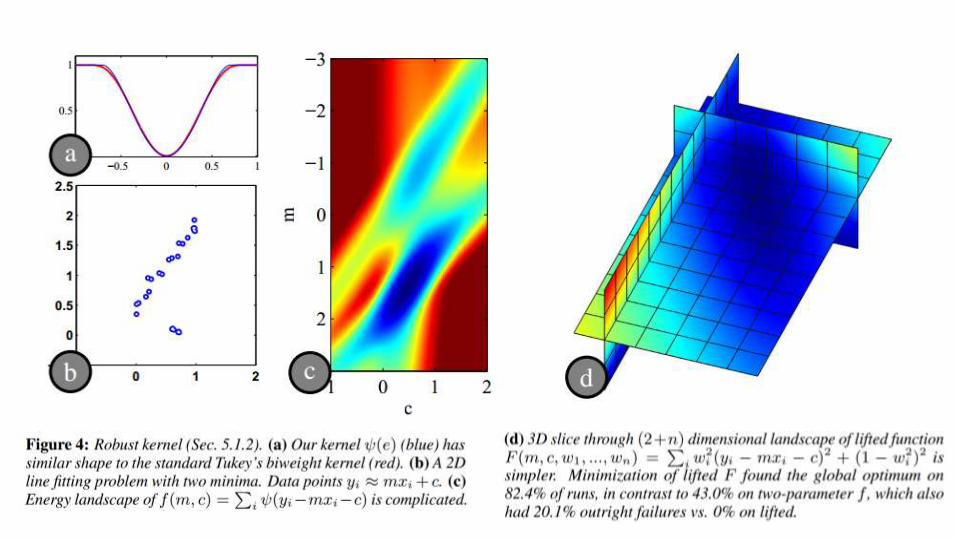
Global minimum in a good place

But hard to optimize:• Multiple optima• Huge flat spots

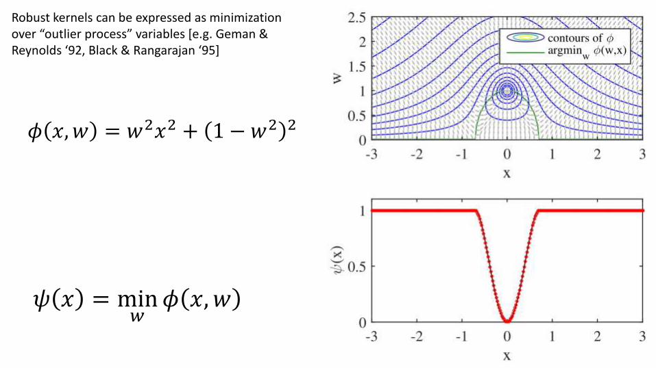
Robust kernels can be expressed as minimization over “outlier process” variables [e.g. Geman & Reynolds ‘92, Black & Rangarajan ‘95]

𝜙 𝑥,𝑤 = 𝑤2𝑥2 + 1 − 𝑤2 2

𝜓 𝑥 = min𝑤

𝜙 𝑥,𝑤

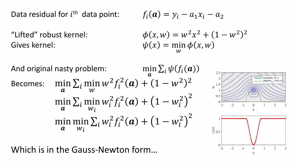
Data residual for 𝑖th data point: 𝑓𝑖 𝒂 = 𝑦𝑖 − 𝑎1𝑥𝑖 − 𝑎2

“Lifted” robust kernel: 𝜙 𝑥,𝑤 = 𝑤2𝑥2 + 1 − 𝑤2 2

Gives kernel: 𝜓 𝑥 = min𝑤

𝜙 𝑥,𝑤

And original nasty problem: min𝒂

σ𝑖𝜓 𝑓𝑖(𝒂)

Becomes: min𝒂

σ𝑖min𝑤𝑤2𝑓𝑖

2 𝒂 + 1 − 𝑤2 2

min𝒂

σ𝑖min𝑤𝑖

𝑤𝑖2𝑓𝑖

2 𝒂 + 1 − 𝑤𝑖2 2

min𝒂

min𝑤𝑖

σ𝑖𝑤𝑖2𝑓𝑖

2 𝒂 + 1 − 𝑤𝑖2 2

Which is in the Gauss-Newton form…

196

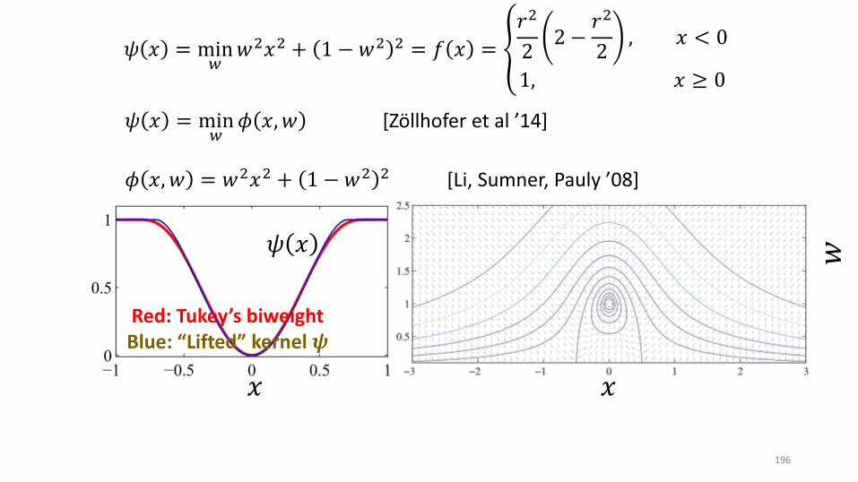
𝜓 𝑥 = min𝑤

𝜙 𝑥,𝑤 [Zöllhofer et al ’14]

𝜙 𝑥, 𝑤 = 𝑤2𝑥2 + 1 − 𝑤2 2 [Li, Sumner, Pauly ’08]

Red: Tukey’s biweightBlue: “Lifted” kernel 𝝍

𝜓 𝑥 = min𝑤

𝑤2𝑥2 + 1 − 𝑤2 2 = 𝑓 𝑥 = ൞

𝑟2

22 −

𝑟2

2, 𝑥 < 0

1, 𝑥 ≥ 0

𝜓 𝑥

𝑥 𝑥

𝑤

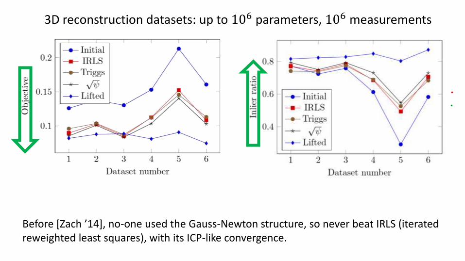
Before [Zach ’14], no-one used the Gauss-Newton structure, so never beat IRLS (iterated reweighted least squares), with its ICP-like convergence.

3D reconstruction datasets: up to 106 parameters, 106 measurements

BUNDLE ADJUSTMENT WITH ROBUST KERNELS 198

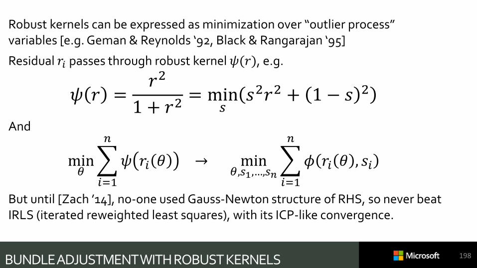
Robust kernels can be expressed as minimization over “outlier process” variables [e.g. Geman & Reynolds ‘92, Black & Rangarajan ‘95]

Residual 𝑟𝑖 passes through robust kernel 𝜓(𝑟), e.g.

𝜓 𝑟 =𝑟2

1 + 𝑟2= min

𝑠𝑠2𝑟2 + 1 − 𝑠 2

And

min𝜃

𝑖=1

𝑛

𝜓 𝑟𝑖 𝜃 → min𝜃,𝑠1,…,𝑠𝑛

𝑖=1

𝑛

𝜙 𝑟𝑖 𝜃 , 𝑠𝑖

But until [Zach ’14], no-one used Gauss-Newton structure of RHS, so never beat IRLS (iterated reweighted least squares), with its ICP-like convergence.

BUNDLE ADJUSTMENT WITH ROBUST KERNELS 199

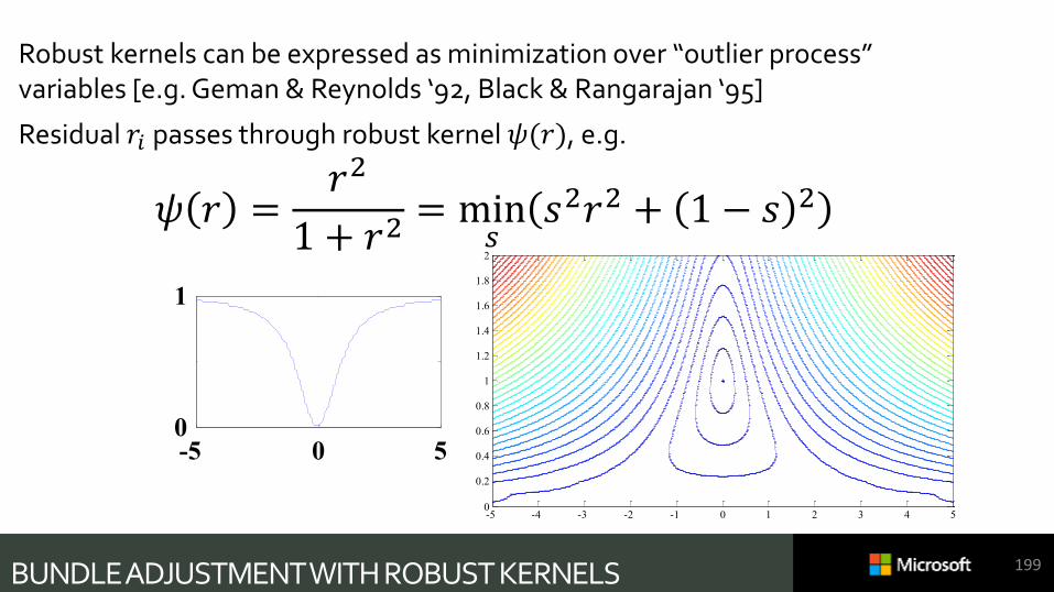
Robust kernels can be expressed as minimization over “outlier process” variables [e.g. Geman & Reynolds ‘92, Black & Rangarajan ‘95]

Residual 𝑟𝑖 passes through robust kernel 𝜓(𝑟), e.g.

𝜓 𝑟 =𝑟2

1 + 𝑟2= min

𝑠𝑠2𝑟2 + 1 − 𝑠 2

-5 0 50

1

-5 -4 -3 -2 -1 0 1 2 3 4 50

0.2

0.4

0.6

0.8

1

1.2

1.4

1.6

1.8

2

0 0.2 0.4 0.6 0.8 10

0.1

0.2

0.3

0.4

0.5

0.6

0.7

0.8

0.9

1

SUBDIV PECULIARITIES 1: PIECEWISE DOMAIN

203

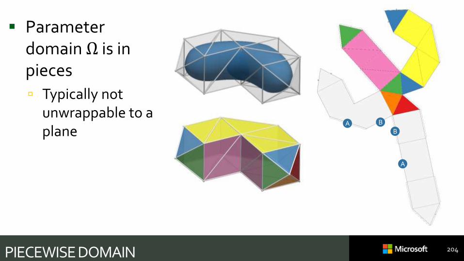
PIECEWISE DOMAIN 204

Parameter domain Ω is in pieces

Typically not unwrappable to a plane

A

A

B

B

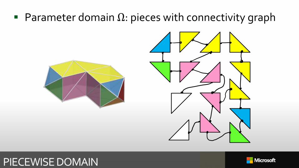
Parameter domain Ω: pieces with connectivity graph

PIECEWISE DOMAIN

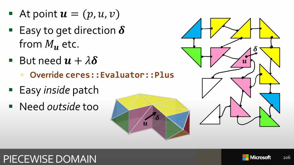
PIECEWISE DOMAIN 206

At point 𝒖 = (𝑝, 𝑢, 𝑣)

Easy to get direction 𝜹from 𝑀𝒖 etc.

But need 𝒖 + 𝜆𝜹 Override ceres::Evaluator::Plus

Easy inside patch

Need outside too

𝒖𝜹

𝒖

𝜹

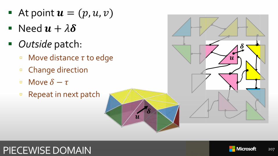
At point 𝒖 = (𝑝, 𝑢, 𝑣)

Need 𝒖 + 𝜆𝜹

Outside patch: Move distance 𝜏 to edge

Change direction

Move 𝛿 − 𝜏

Repeat in next patch

PIECEWISE DOMAIN 207

𝒖𝜹

𝒖

𝜹

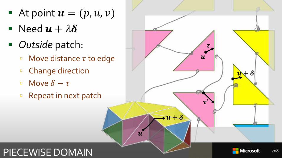
At point 𝒖 = (𝑝, 𝑢, 𝑣)

Need 𝒖 + 𝜆𝜹

Outside patch: Move distance 𝜏 to edge

Change direction

Move 𝛿 − 𝜏

Repeat in next patch

PIECEWISE DOMAIN 208

𝒖

𝒖 + 𝜹

𝝉

𝝉′

𝒖 + 𝜹

𝒖

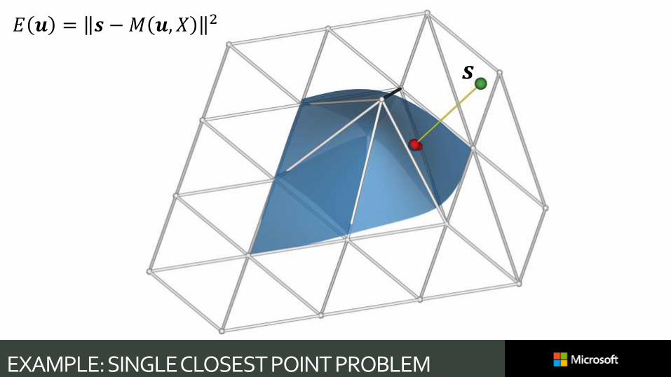
𝐸 𝒖 = 𝒔 −𝑀 𝒖, 𝑋 2

EXAMPLE: SINGLE CLOSEST POINT PROBLEM

𝒔

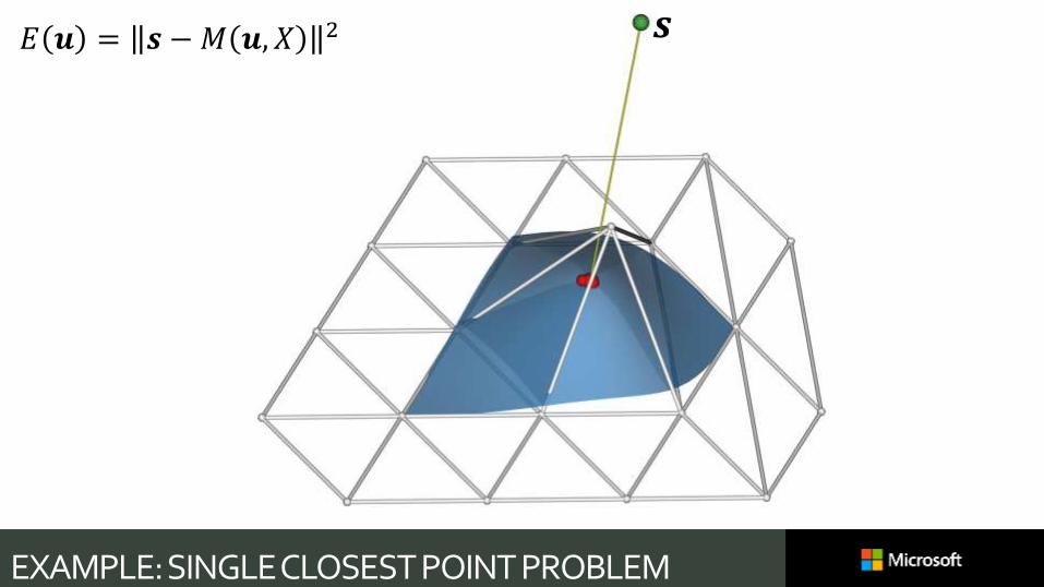
EXAMPLE: SINGLE CLOSEST POINT PROBLEM

𝒔𝐸 𝒖 = 𝒔 −𝑀 𝒖, 𝑋 2

SUBDIV PECULIARITIES 2: EXTRAORDINARY VERTICES

211

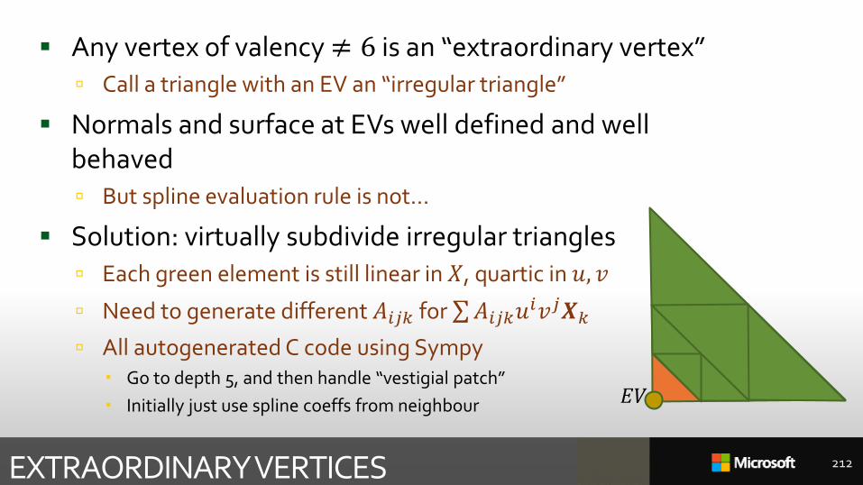
Any vertex of valency ≠ 6 is an “extraordinary vertex” Call a triangle with an EV an “irregular triangle”

Normals and surface at EVs well defined and well behaved But spline evaluation rule is not…

Solution: virtually subdivide irregular triangles Each green element is still linear in 𝑋, quartic in 𝑢, 𝑣

Need to generate different 𝐴𝑖𝑗𝑘 for σ𝐴𝑖𝑗𝑘𝑢𝑖𝑣𝑗𝑿𝑘

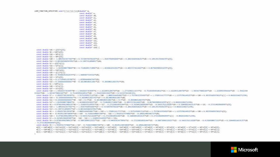
All autogenerated C code using Sympy Go to depth 5, and then handle “vestigial patch”

Initially just use spline coeffs from neighbour

EXTRAORDINARY VERTICES 212

𝐸𝑉

SUBDIV PECULIARITIES 2: VANISHING DERIVATIVES

214

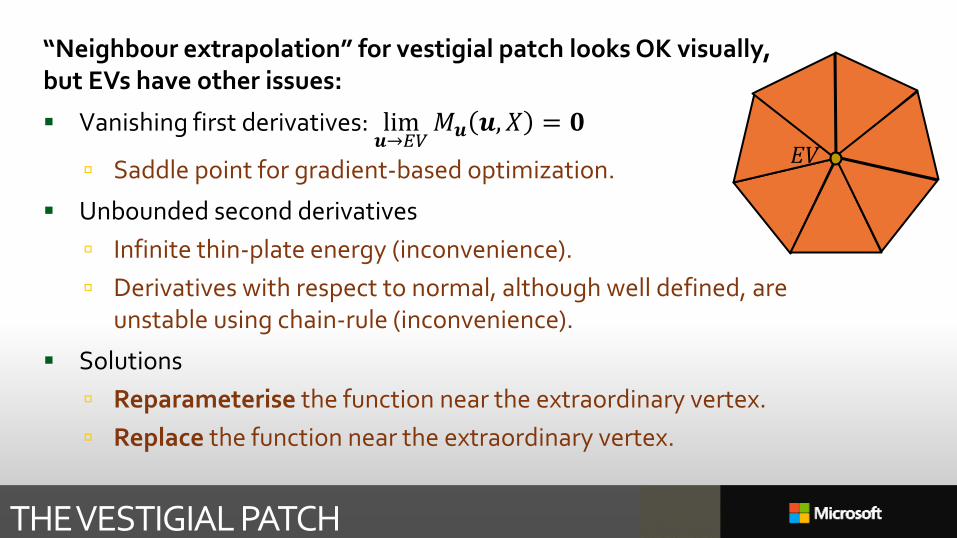
“Neighbour extrapolation” for vestigial patch looks OK visually, but EVs have other issues:

Vanishing first derivatives: lim𝒖→𝐸𝑉

𝑀𝒖 𝒖,𝑋 = 𝟎

Saddle point for gradient-based optimization.

Unbounded second derivatives

Infinite thin-plate energy (inconvenience).

Derivatives with respect to normal, although well defined, are unstable using chain-rule (inconvenience).

Solutions

Reparameterise the function near the extraordinary vertex.

Replace the function near the extraordinary vertex.

THE VESTIGIAL PATCH

𝐸𝑉

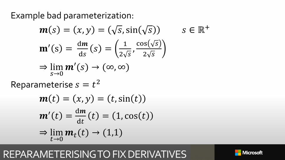
REPARAMETERISING TO FIX DERIVATIVES

Example bad parameterization:

𝒎 𝑠 = 𝑥, 𝑦 = 𝑠, sin 𝑠 𝑠 ∈ ℝ+

𝐦′ s =d𝒎

d𝑠𝑠 =

1

2 𝑠,cos 𝑠

2 𝑠

⇒ lim𝑠→0

𝒎′(𝑠) → (∞,∞)

Reparameterise 𝑠 = 𝑡2

𝒎 𝑡 = 𝑥, 𝑦 = 𝑡, sin 𝑡

𝒎′ 𝑡 =d𝒎

d𝑡𝑡 = 1, cos 𝑡

⇒ lim𝑡→0

𝒎𝑡(𝑡) → (1,1)

Using subdivs is easy The messy stuff is encapsulated in Eval_M*(), and Plus()

Google’s “Ceres” solver does all the Levenberg-Marquardt

Continuous optimization often doesn’t need a very good initial estimate

Using subdivs allows correspondences 𝒖𝑖 to update during the optimization If ICP takes a long time, this may not…

But you must exploit sparsity

Future work: Dogs, hinted ARAP, skeleton, even more speed, …

CONCLUSIONS ETC 217

Seen a few students nastily bitten by collapsing meshes

So what’s changed? How do I get bitten by the bug, not the hornet?1. Sum over data, not model

2. Use modern (2006) regularizers

3. Vary everything

4. Define clean interpolants

FITTING MESHES 218

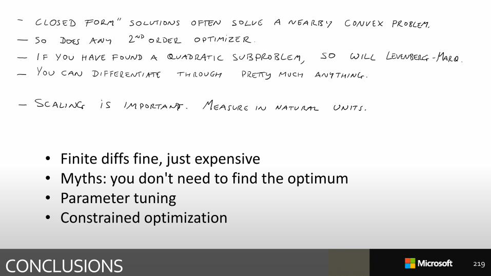
CONCLUSIONS 219

• Finite diffs fine, just expensive• Myths: you don't need to find the optimum• Parameter tuning• Constrained optimization