Direct Least Squares Fitting of Ellipses

Andrew W. Fitzgibbon Maurizio Pilu

Robert B. Fisher

Department of Arti�cial Intelligence

The University of Edinburgh

5 Forrest Hill, Edinburgh EH1 2QL

SCOTLAND

email: fandrewfg,maurizp,rbfg@aifh.ed.ac.uk

January 4, 1996

Abstract

This work presents a new e�cient method for �tting ellipses to scattered data.

Previous algorithms either �tted general conics or were computationally expensive.

By minimizing the algebraic distance subject to the constraint 4ac� b2 = 1 the new

method incorporates the ellipticity constraint into the normalization factor. The new

method combines several advantages: (i) It is ellipse-speci�c so that even bad data

will always return an ellipse; (ii) It can be solved naturally by a generalized eigensys-

tem and (iii) it is extremely robust, e�cient and easy to implement. We compare the

proposed method to other approaches and show its robustness on several examples in

which other non-ellipse-speci�c approaches would fail or require computationally ex-

pensive iterative re�nements. Source code for the algorithm is supplied and a demon-

stration is available on http://www.dai.ed.ac.uk/groups/mvu/ellipse-demo.html

1 Introduction

The �tting of primitive models to image data is a basic task in pattern recognition and

computer vision, allowing reduction and simpli�cation of the data to the bene�t of higher

level processing stages. One of the most commonly used models is the ellipse which,

being the perspective projection of the circle, is of great importance for many industrial

applications. Despite its importance, however, there has been until now no computationally

e�cient ellipse-speci�c �tting algorithm [13, 4].

1

In this paper we introduce a new method of �tting ellipses, rather than general conics,

to segmented data. As we shall see in the next section, current methods are either com-

putationally expensive Hough transform-based approaches, or perform ellipse �tting by

least-squares �tting to a general conic and rejecting non-elliptical �ts. These latter meth-

ods are cheap and perform well if the data belong to a precisely elliptical arc with little

occlusion but su�er from the major shortcoming that under less ideal conditions | non-

strictly elliptical data, moderate occlusion or noise | they often yield unbounded �ts to

hyperbolae. In a situation where ellipses are speci�cally desired, such �ts must be rejected

as useless. A number of iterative re�nement procedures [15, 7, 10] alleviate this problem,

but do not eliminate it. In addition, these techniques often increase the computational

burden unacceptably.

This paper introduces a new �tting method that combines the following advantages:

� Ellipse-speci�city, providing useful results under all noise and occlusion conditions.

� Invariance to Euclidean transformation of the data.

� High robustness to noise.

� High computational e�ciency.

After a description of previous algebraic �tting methods, in Section 3 we describe the

method and provide a theoretical analysis of the uniqueness of the elliptical solution.

Section 4 contains experimental results, notably to highlight noise resilience, invariance

properties and behaviour for non-elliptical data. We conclude by presenting some possible

extensions.

2 Previous Methods and their Limitations

The literature on ellipse �tting divides into two general techniques: clustering and least-

squares �tting.

Clustering methods are based on mapping sets of points to the parameter space, such as

the Hough transform [9, 18] and accumulation methods [12]. These Hough-like techniques

have some great advantages, notably high robustness to occlusion and no requirement

2

Bookstein Method Ellipse−Specific Method

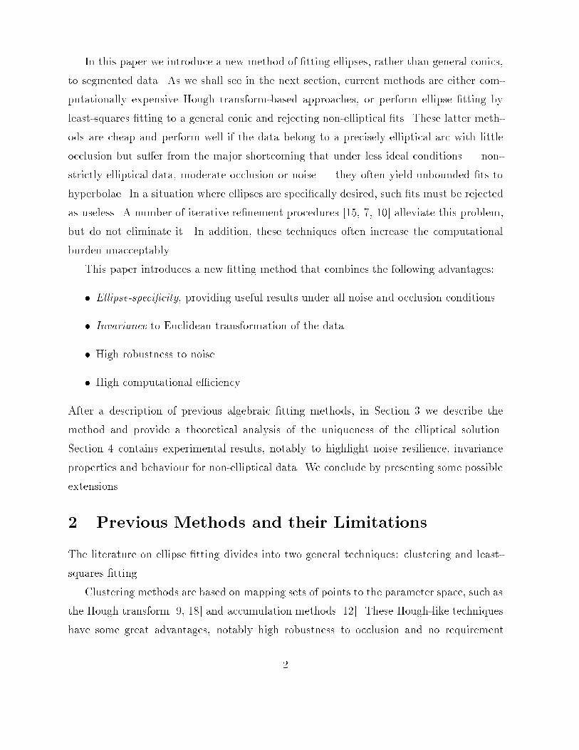
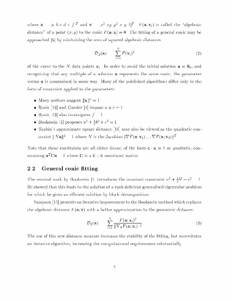
Figure 1: Speci�city to ellipses: the solutions are shown for Bookstein's and our method.In the case of the Bookstein algorithm, the solid line corresponds to the global minimum,while the dotted lines are the other two local minima. The ellipse-speci�c algorithm has asingle minimum.

for pre-segmentation, but they su�er from the great shortcomings of high computational

complexity and non-uniqueness of solutions, which can render them unsuitable for real

applications. Particularly when curves have been pre-segmented, their computational cost

is signi�cant.

Least-squares techniques center on �nding the set of parameters that minimize some

distance measure between the data points and the ellipse. In this section we brie y present

the most cited works in ellipse �tting and its closely related problem, conic �tting. It will

be shown that the direct speci�c least-square �tting of ellipses has, up to now, not been

solved.

2.1 Problem statement

Before reviewing the literature on general conic �tting, we will introduce a statement of

the problem that allows us to unify several approaches under the umbrella of constrained

least squares. Let us represent a general conic by an implicit second order polynomial:

F (a;x) = a � x = ax2 + bxy + cy2 + dx+ ey + f = 0; (1)

3

where a = [a b c d e f ]T and x = [x2 xy y2 x y 1]T . F (a;xi) is called the \algebraic

distance" of a point (x; y) to the conic F (a;x) = 0. The �tting of a general conic may be

approached [6] by minimizing the sum of squared algebraic distances

DA(a) =NXi=1

F (xi)2 (2)

of the curve to the N data points xi. In order to avoid the trivial solution a = 06, and

recognizing that any multiple of a solution a represents the same conic, the parameter

vector a is constrained in some way. Many of the published algorithms di�er only in the

form of constraint applied to the parameters:

� Many authors suggest kak2 = 1.

� Rosin [13] and Gander [4] impose a+ c = 1.

� Rosin [13] also investigates f = 1.

� Bookstein [1] proposes a2 + 1

2b2 + c2 = 1.

� Taubin's approximate square distance [16] may also be viewed as the quadratic con-

straint kNak2 = 1 where N is the Jacobian [rF (a;x1) : : :rF (a;xN)]T .

Note that these constraints are all either linear, of the form c � a = 1 or quadratic, con-

straining aTCa = 1 where C is a 6� 6 constraint matrix.

2.2 General conic �tting

The seminal work by Bookstein [1] introduces the invariant constraint a2 + 1

2b2 + c2 = 1.

He showed that this leads to the solution of a rank-de�cient generalised eigenvalue problem

for which he gives an e�cient solution by block decomposition.

Sampson [15] presents an iterative improvement to the Bookstein method which replaces

the algebraic distance F (a;x) with a better approximation to the geometric distance:

DS(a) =NXi=1

F (a;xi)2

krxF (a;xi)k2(3)

The use of this new distance measure increases the stability of the �tting, but necessitates

an iterative algorithm, increasing the computational requirements substantially.

4

Taubin [16] proposed an approximation of (3) as

DT (a) �

PN

i=1 F (a;xi)2PN

i=1 krxF (a;xi)k2; (4)

which, while strictly valid only for a circle, again allows the problem to be expressed as

a generalized eigensystem, reducing the computational requirements back to the order of

Bookstein's process.

2.3 Towards ellipse-speci�c �tting

A number of papers have concerned themselves with the speci�c problem of recovering

ellipses rather than general conics. Bookstein's method does not restrict the �tting to be

an ellipse, in the sense that given arbitrary data the algorithm can return an hyperbola or

a parabola, even from elliptical input, but it has been widely used in the past decade.

Porrill [10] and Ellis et al. [2] use Bookstein's method to initialize a Kalman �lter.

The Kalman �lter iteratively minimizes the gradient distance (3) in order to gather new

image evidence and to reject non-ellipse �ts by testing the discriminant b2 � 4ac < 0 at

each iteration. Porrill also gives nice examples of the con�dence envelopes of the �ttings.

Rosin [13] also uses a Kalman Filter, and in [14] he restates that ellipse-speci�c �tting is

a non-linear problem and that iterative methods must be employed. He also [13] analyses

the pro and cons of two commonly used normalizations, f = 1 and a + c = 1 and shows

that the former biases the �tting to have smaller eccentricity, therefore increasing the

probability of returning an ellipse, at the cost of losing transformational invariance.

Although these methods transform the disadvantage of having a non-speci�c ellipse

�tting method into an asset by using the ellipse constraint to check whether new data has

to be included or to assess the quality of the �t, the methods require many iterations in

the presence of very bad data, and may fail to converge in extreme cases.

Recently Gander et al. [4] published a paper entitled \Least-square �tting of ellipses

and circles" in which the normalization a+ c = 1 leads to an over-constrained system of

N linear equations. The proposed normalization is the same as that in [10, 14] and it does

not force the �tting to be an ellipse (the hyperbola 3x2 � 2y2 = 0 satis�es the constraint).

It must be said, however, that in the paper they make no explicit claim that the algorithm

is ellipse speci�c.

5

Haralick [6, x11.10.7] takes a di�erent approach. E�ectively, he guarantees that the

conic is an ellipse by replacing the coe�cients fa; b; cgwith new expressions fp2; 2pq; q2+r2g

so that the discriminant b2�4ac becomes �4p2r2 which is guaranteed negative. Minimiza-

tion over the space fp; q; r; d; e; fg then yields an ellipse. His algorithm is again iterative,

and an initial estimate is provided by a method of moments. Keren et al. [8] apply a

similar technique to Haralick's and extend the method to the �tting of bounded quartic

curves. Again, their algorithm is iterative.

In the following sections we will refer for comparisons to the methods of Bookstein,

Gander and Taubin.

3 Direct ellipse-speci�c �tting

In order to �t ellipses speci�cally while retaining the e�ciency of solution of the linear

least-squares problem (2), we would like to constrain the parameter vector a so that the

conic that it represents is forced to be an ellipse. The appropriate constraint is well known,

namely that the discriminant b2 � 4ac be negative. However, this constrained problem is

di�cult to solve in general as the Kuhn-Tucker conditions [11] do not guarantee a solution.

In fact, we have not been able to locate any reference regarding the minimization of a

quadratic form subject to such a nonconvex inequality.

Although imposition of this inequality constraint is di�cult in general, in this case

we have the freedom to arbitrarily scale the parameters so we may simply incorporate

the scaling into the constraint and impose the equality constraint 4ac� b2 = 1. This is a

quadratic constraint which may be expressed in the matrix form aTCa = 1 as

aT

26664

0 0 2 0 0 00 �1 0 0 0 02 0 0 0 0 00 0 0 0 0 00 0 0 0 0 00 0 0 0 0 0

37775a = 1 (5)

3.1 Solution of the quadratically constrained minimization

Following Bookstein [1], the constrained �tting problem is:

Minimize E = kDak2, subject to the constraint aTCa = 1 (6)

6

where the design matrix D is the n � 6 matrix [x1 x2 � � � xn]T . Introducing the Lagrange

multiplier � and di�erentiating we arrive at the system of simultaneous equations1

2DTDa� 2�Ca = 0aTCa = 1

(7)

This may be rewritten as the system

Sa = �Ca (8)

aTCa = 1 (9)

where S is the scatter matrix DTD. This system is readily solved by considering the

generalized eigenvectors of (8). If (�i;ui) solves (8) then so does (�i; �ui) for any � and

from (9) we can �nd the value of �i as �2iu

Ti Cui = 1 giving

�i =

s1

uTi Cui=

s�i

uTi Sui(10)

Finally, setting ai = �iui solves (7). As in general there may be up to 6 real solutions, the

solution is chosen that yields the lowest residual aTi Sai = �i.

We note that the solution of the eigensystem (8) gives 6 eigenvalue-eigenvector pairs

(�i;ui). Each of these pairs gives rise to a local minimum if the term under the square root

in (10) is positive. In general, S is positive de�nite, so the denominator uTi Sui is positive

for all ui. Therefore the square root exists if �i > 0, so any solutions to (7) must have

positive generalized eigenvalues.

3.2 Analysis of the constraint 4ac� b2 = 1

Now we show that the minimization of kDak2 subject to 4ac� b2 = 1 yields exactly one

solution (which corresponds, by virtue of the constraint, to an ellipse). For the demonstra-

tion, we will require the following lemma (proved in the appendix):

Lemma 1 The signs of the generalized eigenvalues of Su = �Cu are the same as those

of the constraint matrix C, up to permutation of the indices.

1Note that the method of Lagrange multipliers is not valid when the gradient of the constraint functionbecomes zero. In (6) this means Ca = 0, but then aTCa = 0 so the constraint is violated and there is nosolution.

7

Theorem 1 The solution of the conic �tting problem (6) admits exactly one elliptical

solution corresponding to the single negative generalized eigenvalue of (8). The solution is

also invariant to rotation and translation of the data points.

Proof:

Since the eigenvalues of C are f�2;�1; 2; 0; 0; 0g, from Lemma 1 we have that (8) has

exactly one positive eigenvalue �i < 0, giving the unique solution a = �iui to (7). As DTD

is positive semide�nite, the constrained problem has a minimum, which must satisfy (7),

and we conclude that a solves the constrained problem. The constraint (5) is a conic

invariant to Euclidean transformation and so is the solution (see [1]) 2

3.3 Remark

Before leaping to the experimental section, there is an important intuitive remark to be

made. An eigenvector of the eigensystem (8) is a local minimizer of the Rayleigh quotient

aTSa

aTCa. In this case the implicit normalization by b2 � 4ac turns singular for b2 � 4ac = 0.

Rosin [13] writes that, not surprisingly, the minimization tends to \pull" the solution away

from singularities; in our case the singularity is a parabola and so the unique elliptical

solution tends to be biased towards low eccentricity, which explains many of the following

results, such as those in Figure 6.

4 Experimental Results

In this section we present experimental results that compare the ellipse-speci�c solution

to previous methods in terms of quality and robustness. We include both quantitative

and qualitative results in order to allow other researchers to evaluate the utility of the

ellipse-speci�c algorithm with respect to the others cited. Fitzgibbon [3] provides further

theoretical and quantitative results for a wide range of conic-�tting algorithms.

4.1 Ellipse-speci�city

Despite the theoretical proof of the algorithm's ellipse-speci�city, it is instructive to observe

its performance on some example data, of which Figure 1 provides an example. There,

all the three generalized eigensolutions of Bookstein's method and ours are shown for the

8

AB

C D

E F G H

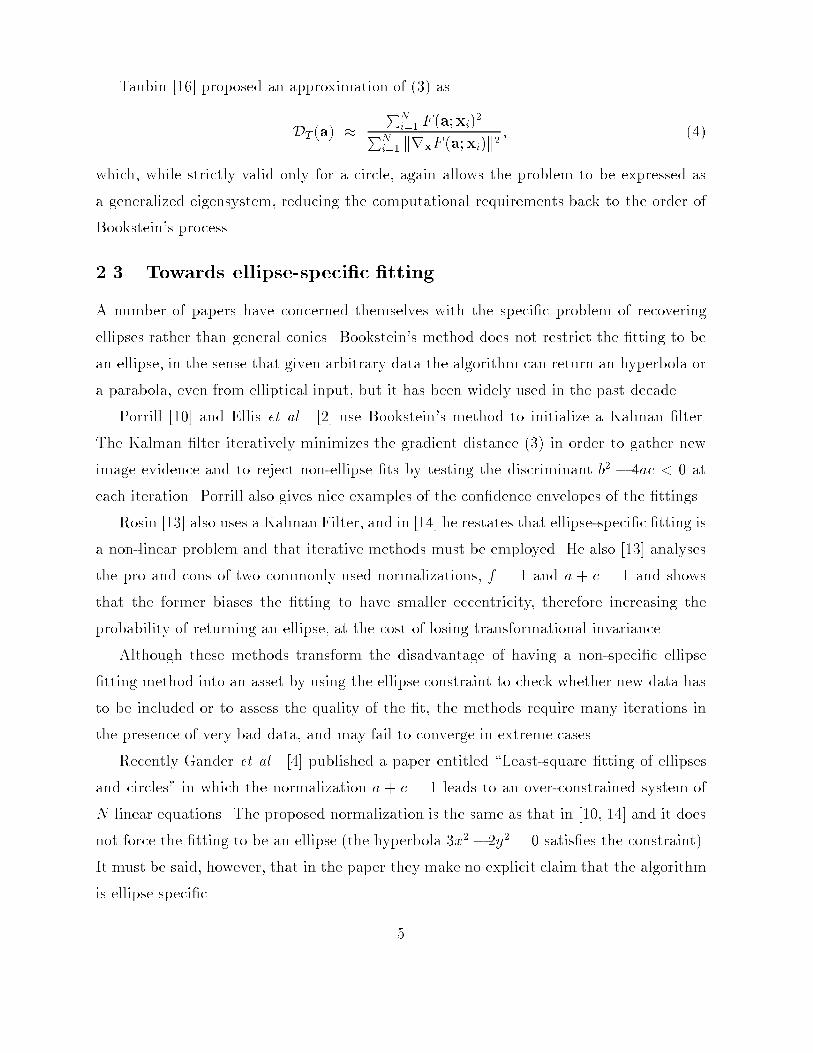
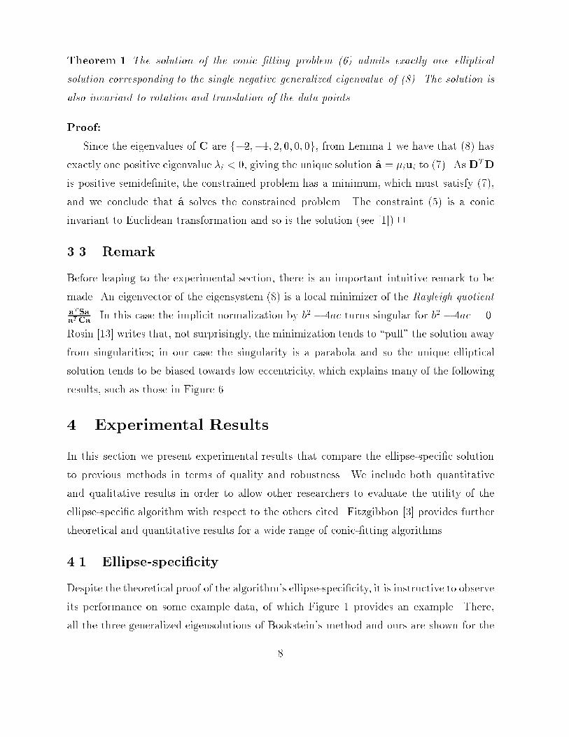
Figure 2: Some hand-drawn data sets. The linetype/algorithm correspondences are Book-stein: dotted; Gander: dashed; Taubin: dash-dot; New: solid.

same set of data. Bookstein's algorithm gives a hyperbola as the best solution which, while

an accurate representation of the data, is of little use if ellipses are sought. In contrast,

the ellipse-speci�c algorithm returns an ellipse as expected.

Figure 2 shows some more examples with hand-drawn datasets. The results of our

method are superimposed on those of Bookstein and Gander. Dataset A is almost elliptical

and indistinguishable �ts were produced. Dataset B is elliptical but more noisy. In C,

Bookstein's method returns a hyperbola while in D and E both Bookstein and Gander

return hyperbolae. In F and G we have a \tilde" and two bent lines. Clearly these are

not elliptical data but illustrate that the algorithm may be useful as an alternative to the

covariance ellipsoid frequently used for coarse data bounding.

4.2 Noise sensitivity

Now we qualitatively assess the robustness of the method to noise and compare it to the

Gander and Taubin algorithms. Taubin's approach yields a more precise estimate but its

ellipse non-speci�city make it unreliable in the presence of noise. We have not included

9

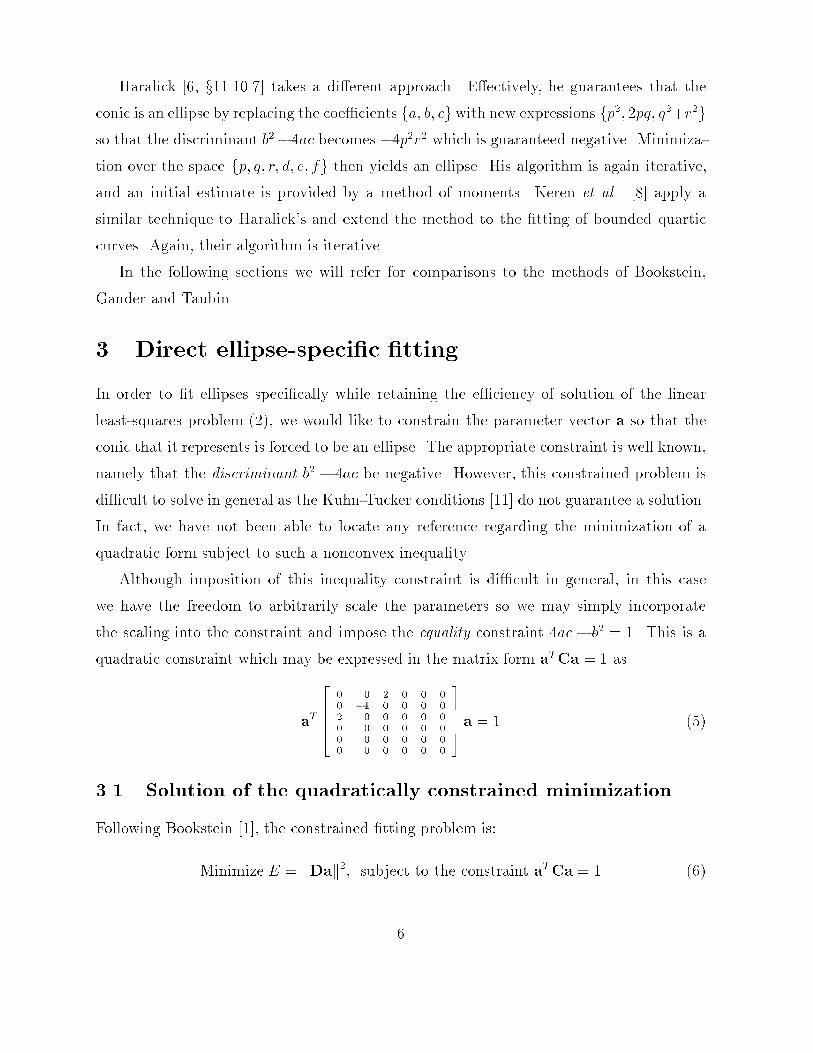
Sigma=0.01 Sigma=0.03 Sigma=0.05 Sigma=0.07 Sigma=0.09 Sigma=0.11 Sigma=0.13 Sigma=0.15 Sigma=0.17 Sigma=0.19

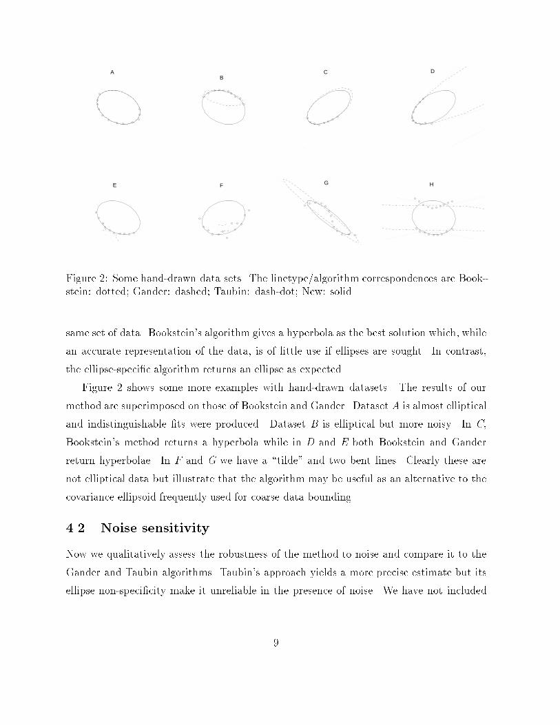
Figure 3: Stability experiments with increasing noise level. Top row: our method; Middlerow: Gander; Bottom row: Taubin

Bookstein's algorithm here as its performance in the presence of noise turned out to be

poorer than Gander's and Taubin's.

We have performed a number of experiments of which we present two, shown in Figures

3 and 4. The data were generated by adding isotropic Gaussian noise to a synthetic elliptical

arc, and presenting each algorithm with the same set of noisy points.

The �rst experiment (Figure 3) illustrates the performance with respect to increasing

noise level. The standard deviation of the noise varies from 0.01 in the leftmost column to

0.19 in the rightmost column; the noise has been set relatively high level because, as shown

in the left-most column, the performance of the three algorithms is substantially the same

at low noise level when given precise elliptical data.

The top row shows the results for the method proposed here. As expected, the �tted

ellipses shrink with increasing levels of high noise; in fact in the limit the elliptical arc

will look like a noisy line. It is worth noticing however that the ellipse dimension degrades

gracefully with the increase of noise level. Shrinking is evident also in the other algorithms,

but the degradation is more erratic as non-elliptical �ts arise.

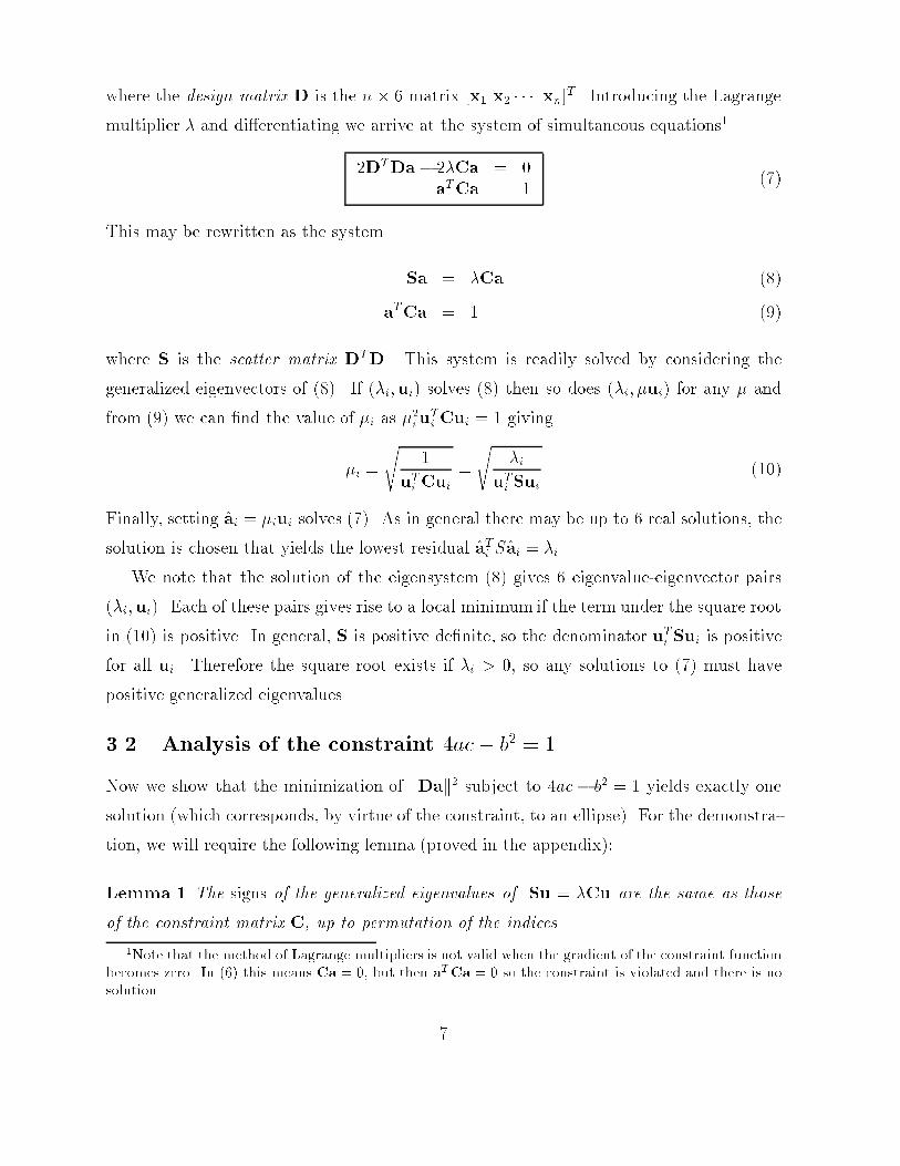
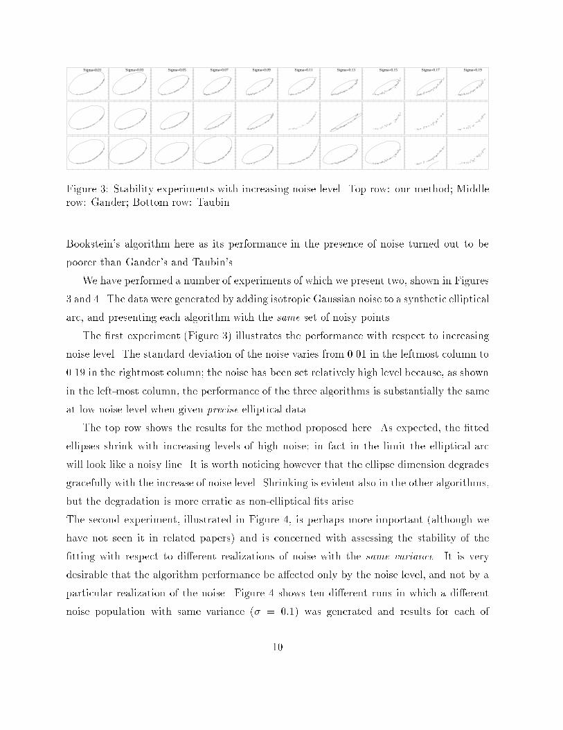
The second experiment, illustrated in Figure 4, is perhaps more important (although we

have not seen it in related papers) and is concerned with assessing the stability of the

�tting with respect to di�erent realizations of noise with the same variance. It is very

desirable that the algorithm performance be a�ected only by the noise level, and not by a

particular realization of the noise. Figure 4 shows ten di�erent runs in which a di�erent

noise population with same variance (� = 0:1) was generated and results for each of

10

Sigma=0.10 Sigma=0.10 Sigma=0.10 Sigma=0.10 Sigma=0.10 Sigma=0.10 Sigma=0.10 Sigma=0.10 Sigma=0.10 Sigma=0.10

Figure 4: Stability experiments for di�erent runs with same noise variance. Top row:proposed method; Mid Row: Gander's Method; Bottom Row: Taubin's method

the three methods is displayed. In this and similar experiments (see also Figure 6) we

found that the stability of the method is noteworthy. Gander's algorithm shows a greater

variation in results and Taubin's, while improving on Gander's, remains less stable than

the proposed algorithm.

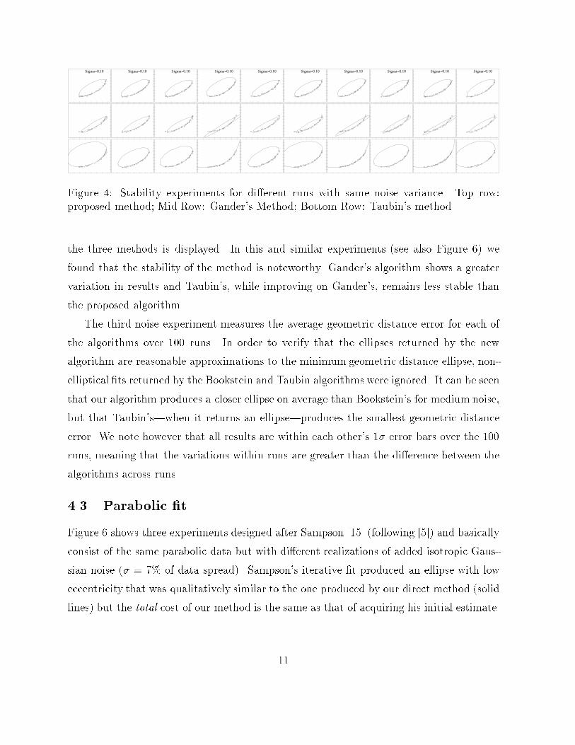
The third noise experiment measures the average geometric distance error for each of

the algorithms over 100 runs. In order to verify that the ellipses returned by the new

algorithm are reasonable approximations to the minimum geometric distance ellipse, non-

elliptical �ts returned by the Bookstein and Taubin algorithms were ignored. It can be seen

that our algorithm produces a closer ellipse on average than Bookstein's for medium noise,

but that Taubin's|when it returns an ellipse|produces the smallest geometric distance

error. We note however that all results are within each other's 1� error bars over the 100

runs, meaning that the variations within runs are greater than the di�erence between the

algorithms across runs.

4.3 Parabolic �t

Figure 6 shows three experiments designed after Sampson [15] (following [5]) and basically

consist of the same parabolic data but with di�erent realizations of added isotropic Gaus-

sian noise (� = 7% of data spread). Sampson's iterative �t produced an ellipse with low

eccentricity that was qualitatively similar to the one produced by our direct method (solid

lines) but the total cost of our method is the same as that of acquiring his initial estimate.

11

10−2

100

10−4

10−2

100

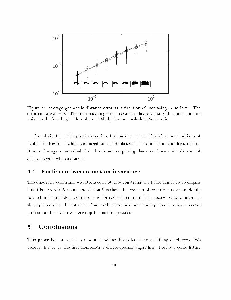
Figure 5: Average geometric distance error as a function of increasing noise level. Theerrorbars are at �1�. The pictures along the noise axis indicate visually the correspondingnoise level. Encoding is Bookstein: dotted; Taubin: dash-dot; New: solid.

As anticipated in the previous section, the low eccentricity bias of our method is most

evident in Figure 6 when compared to the Bookstein's, Taubin's and Gander's results.

It must be again remarked that this is not surprising, because those methods are not

ellipse-speci�c whereas ours is.

4.4 Euclidean transformation invariance

The quadratic constraint we introduced not only constrains the �tted conics to be ellipses

but it is also rotation and translation invariant. In two sets of experiments we randomly

rotated and translated a data set and for each �t, compared the recovered parameters to

the expected ones. In both experiments the di�erence between expected semi-axes, centre

position and rotation was zero up to machine precision.

5 Conclusions

This paper has presented a new method for direct least square �tting of ellipses. We

believe this to be the �rst noniterative ellipse-speci�c algorithm. Previous conic �tting

12

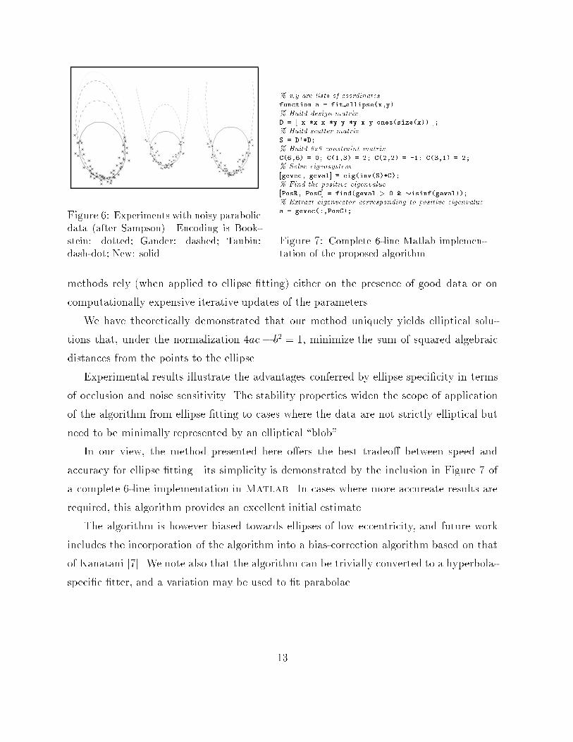
Figure 6: Experiments with noisy parabolic

data (after Sampson). Encoding is Book-

stein: dotted; Gander: dashed; Taubin:

dash-dot; New: solid.

% x,y are lists of coordinates

function a = fit ellipse(x,y)

% Build design matrix

D = [ x.*x x.*y y.*y x y ones(size(x)) ];

% Build scatter matrix

S = D'*D;

% Build 6x6 constraint matrix

C(6,6) = 0; C(1,3) = 2; C(2,2) = -1; C(3,1) = 2;

% Solve eigensystem

[gevec, geval] = eig(inv(S)*C);

% Find the positive eigenvalue

[PosR, PosC] = find(geval > 0 & �isinf(geval));

% Extract eigenvector corresponding to positive eigenvalue

a = gevec(:,PosC);

Figure 7: Complete 6-line Matlab implemen-

tation of the proposed algorithm.

methods rely (when applied to ellipse �tting) either on the presence of good data or on

computationally expensive iterative updates of the parameters.

We have theoretically demonstrated that our method uniquely yields elliptical solu-

tions that, under the normalization 4ac� b2 = 1, minimize the sum of squared algebraic

distances from the points to the ellipse.

Experimental results illustrate the advantages conferred by ellipse speci�city in terms

of occlusion and noise sensitivity. The stability properties widen the scope of application

of the algorithm from ellipse �tting to cases where the data are not strictly elliptical but

need to be minimally represented by an elliptical \blob".

In our view, the method presented here o�ers the best tradeo� between speed and

accuracy for ellipse �tting|its simplicity is demonstrated by the inclusion in Figure 7 of

a complete 6-line implementation in Matlab. In cases where more accureate results are

required, this algorithm provides an excellent initial estimate.

The algorithm is however biased towards ellipses of low eccentricity, and future work

includes the incorporation of the algorithm into a bias-correction algorithm based on that

of Kanatani [7]. We note also that the algorithm can be trivially converted to a hyperbola-

speci�c �tter, and a variation may be used to �t parabolae.

13

6 Acknowledgements

The second author is partially sponsored by SGS-THOMSON Microelectronics UK. This

work was partially funded by UK EPSRC Grant GR/H/86905.

References

[1] F.L. Bookstein. Fitting conic sections to scattered data. Computer Graphics and Image

Processing, (9):56{71, 1979.

[2] T. Ellis, A. Abbood, and B. Brillault. Ellipse detection and matching with uncertainty.

Image and Vision Computing, 10(2):271{276, 1992.

[3] A.W. Fitzgibbon and R.B. Fisher. A buyer's guide to conic �tting. In Proceedings of British

Machine Vision Conference, Birmingam, 1995.

[4] W. Gander, G.H. Golub, and R. Strebel. Least-square �tting of circles and ellipses. BIT,

(43):558{578, 1994.

[5] R. Gnanadesikan. Methods for statistical data analysis of multivariate observations. John

Wiley & sons, New York, 1977.

[6] R. M. Haralick and L. G. Shapiro. Computer and Robot Vision, volume 1. Addison-Wesley,

1993.

[7] K. Kanatani. Statistical bias of conic �tting and renormalization. IEEE T-PAMI, 16(3):320{

326, 1994.

[8] D. Keren, D. Cooper, and J. Subrahmonia. Describing complicated objects by implicit

polynomials. IEEE T-PAMI, 16(1):38{53, 1994.

[9] V.F. Leavers. Shape Detection in Computer Vision Using the Hough Transform. Springer-

Verlag, 1992.

[10] J. Porrill. Fitting ellipses and predicting com�dence envelopes using a bias corrected Kalman

�lter. Image and Vision Computing, 8(1), February 1990.

[11] S. S. Rao. Optimization: Theory and Applications. Wiley Eastern, 2 edition, 1984.

[12] P. L. Rosin. Ellipse �tting by accumulating �ve-point �ts. Pattern Recognition Letters,

(14):661{699, August 1993.

[13] P.L. Rosin. A note on the least square �tting of ellipses. Pattern Recognition Letters,

(14):799{808, October 1993.

[14] P.L. Rosin and G.A. West. Segmenting curves into lines and arcs. In Proceedings of the

Third International Conference on Computer Vision, pages 74{78, Osaka, Japan, December

1990.

14

[15] P.D. Sampson. Fitting conic sections to very scattered data: An iterative re�nement of the

Bookstein algorithm. Computer Graphics and Image Processing, (18):97{108, 1982.

[16] G. Taubin. Estimation of planar curves, surfaces and non-planar space curves de�ned by

implicit equations , with applications to edge and range image segmentation. IEEE PAMI,

13(11):1115{1138, November 1991.

[17] J. H. Wilkinson. The algebraic eigenvalue problem. Claredon Press, Oxford, England, 1965.

[18] H. K. Yuen, J. Illingworth, and J. Kittler. Detecting partially occluded ellipses using the

Hough transform. Image and Vision Computing, 7(1):31{37, 1989.

Appendix

Lemma 1 The signs of the generalized eigenvalues of

Su = �Cu (11)

where S 2 <n�n is positive de�nite, and C 2 <n�n is symmetric, are the same as those of

the matrix C, up to permutation of the indices.

Let us de�ne the spectrum �(S) as the set of eigenvalues of S. Let us analogously de�ne

�(S;C) to be the set of generalized eigenvalues of (11). The inertia i(S) is de�ned as the

set of signs of �(C), and we correspondingly de�ne i(S;C). Then the lemma is equivalent

to proving that i(S;C) = i(C).

As S is positive de�nite, it may be decomposed as Q2 for symmetric Q, allowing us to

write (11) as

Q2u = �Cu

Now, substituting v = Qu and premultiplying by Q�1 gives

v = �Q�1CQ�1v

so that �(S;C) = �(Q�1CQ�1)�1 and thus i(S;C) = i(Q�1CQ�1).

From Sylvester's Law of Inertia [17] we have that for any symmetric S and nonsingular X,

i(S) = i(XTSX)

Therefore, substituting X = XT = Q�1 we have i(C) = i(Q�1CQ�1) = i(S;C). 2

15