Firm Responses to Book Income

Alternative Minimum Taxes ∗

Jordan Richmond, Princeton University, December 23, 2020

Abstract

How do firms respond to book income alternative minimum taxes (AMTs)? I answerthis question using a differences-in-differences approach, studying firm responses to theAMT book income adjustment in 1987. Firms manage their earnings to avoid the tax,corresponding to a three-year book income elasticity of 3.62 and six-year elasticity of3.21, but do not exhibit significant real production or investment responses. A revenuescoring exercise applying firm avoidance responses suggests modern book income AMTproposals would raise substantial tax revenue and that many third party scores of bookincome AMTs are inconsistent with estimates of firm responses.

∗I thank Owen Zidar and Ilyana Kuziemko for helpful comments. All errors are my own.

1

“You cannot go to a mill where somebody is making $20,000 a year and attempt toexplain to them why a major American corporation can have over $1 billion in profitsand pay no taxes.” – Senator Bob Packwood1

Profitable firms with very small tax bills often face public ire. Over the last forty years

in the United States, tax policymakers have attempted to eliminate the divergence of some

firms’ incomes and tax liabilities by imposing alternative minimum taxes (AMTs). Despite

these attempts, firms continue to find ways to simultaneously take in large profits and pay

very little in taxes. For example, in 2017, Amazon reported $5.6 billion in profit but paid

$0 in taxes (Gardner, 2020).

The existence of profitable firms with small tax bills like Amazon undermine public

perceptions of a fair tax code. Profitable firms can owe small tax bills because the tax

code includes deductions and credits meant to incentivize productive economic behavior,

but disproportionate use of these incentives can eliminate all tax liabilities for profitable

firms. AMTs assign a lower tax rate to a broader tax base that excludes many deductions

and credits. Therefore, AMTs introduce limitations on economic incentives built into the

tax code in an attempt to raise revenue from profitable firms and bolster public perceptions

of tax code fairness.

In both the United States and global OECD talks, recent tax proposals have included an

AMT based on book income, the income firms report on their financial statements. These

proposals may be appealing because book income provides a broad tax base, suggesting a

book income AMT could effectively raise revenue from profitable firms that pay few taxes.

However, a book income AMT’s capacity to raise revenue may be limited by tax avoidance

because firms have substantial discretion to determine their own book incomes (Manzon and

Plesko, 2002), while broadening the tax base could lead firms to make inefficient changes to

their production and investment policies.

In this paper, I estimate firm responses to a book income AMT by exploiting variation

in the minimum tax rate on book income introduced by the alternative minimum tax book

income adjustment (AMTBIA87) in 1987. AMTBIA87 is the only historical example in the

U.S. of an AMT that incorporates book income into the tax base. I use a differences-in-

differences empirical strategy that compares firms more likely to be subject to the AMT on

1U.S. Senate Finance Committee Hearing. May 3, 1995. “Alternative Minimum Tax”.

2

book income (treatment) to firms less likely to face the new AMT (control), dividing firms

into treatment and control groups based on their effective tax rates in 1986. This empirical

approach identifies firm responses off the difference in the evolution of outcomes for firms

that are more or less likely to face the book income AMT, assuming that their outcomes

would have evolved similarly in the absence of the policy.

Using Compustat data, I find strong evidence that firms manage their earnings to avoid

AMTBIA87. My preferred point estimates suggest that over a three-year time horizon the

elasticity of book income with respect to the net of tax rate is 3.62, while over a six-year

time horizon the elasticity of book income is 3.21. I measure firm’s earnings management

responses using book tax differences, which reflect discretionary changes firms can make to

their book incomes while holding fixed investment and production responses.

Robustness checks indicate that my estimates of tax avoidance are unlikely to be driven

by mean reversion or simultaneous tax policy changes included in the Tax Reform Act of

1986 (TRA86). Placebo differences-in-differences series that split firms into treatment and

control groups based on effective tax rates in earlier tax years exhibit book tax difference

spikes in the year of the split that revert to 1985 levels in the subsequent year, suggesting

mean reversion is unlikely to drive the results. Meanwhile, TRA86 included concurrent tax

policy changes that reduced the corporate rate and increased the cost of capital - reforms

that a priori might have differential impacts across firms in the treatment and control groups

based on different industry, firm size and effective tax rate compositions. However, various

difference-in-difference specifications flexibly controlling for these firm characteristics all yield

similar estimates of tax avoidance.

This paper adds to a substantial literature that uses accounting or tax data to esti-

mate earnings management responses to AMTBIA87 (Gramlich, 1991; Dhaliwal and Wang,

1992; Boynton, Dobbins and Plesko, 1992; Manzon, 1992; Wang, 1994; Choi, Gramlich and

Thomas, 2001). AMTBIA87 was announced in 1986 but not implemented until 1987, creating

an opportunity for firms to shift book income out of the period the tax was in effect and into

1986. Therefore, earlier work focused on measuring two possible responses to AMTBIA87,

strategic shifting of book income out of 1987 and into 1986 to avoid the tax altogether, and

book income decreases in 1987 to reduce tax liability. While the earlier literature established

3

a consensus that firms decreased their book incomes in 1987, substantial debate persisted

over the presence and magnitude of book income increases in 1986.

This paper builds on the earlier AMTBIA87 literature in four ways. First, I show that

previous studies underestimate book income elasticities by not accounting for pre-trends.

Second, I estimate firm responses over a longer time frame from 1986-1992, finding that

avoidance responses stabilize over a four- to six-year time horizon. Third, I show that any

perceived book income shifting into 1986 can be attributed to selection in the treatment defi-

nition rather than tax avoidance. Finally, I explore heterogeneity across firm sizes, industries,

and tax exposure intensities to shed light on mechanisms underlying firm responses.

Additional differences-in-differences estimates show that firms are unlikely to respond to

a book income AMT by modifying their production or investment policies. Using revenues,

costs of inputs, investment and debt as outcomes, I fail to reject the null hypothesis of zero

response to AMTBIA87 in any year from 1987-1992 for all four outcomes. Complementary

instrumental variables analysis suggests that increases in total tax liability stemming from

AMTBIA87 increase tax revenues, but have no impact on firm revenue, costs of inputs,

investment or debt.

The estimates of tax avoidance and lack of evidence for investment and production

changes in this paper are consistent with economic models of firm responses to taxation

suggesting that, if possible, firms will evade or avoid taxes before making real economic

changes. Existing research on minimum tax schemes in Pakistan, Hungary, Guatemala and

Honduras emphasizes that firms evade minimum taxes by overreporting costs rather than

by making changes to production or investment (Best, Brockmeyer, Kleven, Spinnewijn and

Waseem, 2015; Mosberger, 2016; Alejos, 2018; Lobel, Scot and Zuniga, 2020). In Costa

Rica, firms over-report costs to escape higher tax rates, and in Spain, firms under-report

revenues to escape increased government scrutiny (Bachas and Soto, Forthcoming; Almunia

and Lopez-Rodriguez, 2018). While the United States is generally thought to have higher

tax enforcement capacity than these other countries, flexibility in accounting standards al-

lows firms to avoid AMTBIA87 the same way they might evade a minimum tax in a lower

enforcement environment.

In light of firm responses to AMTBIA87, contemporary proposals to implement a book

4

income AMT will accomplish their goals if they successfully raise revenue from profitable

firms with low tax bills despite firms’ tax avoidance responses. To evaluate the implications

of the earnings management that I estimate in response to AMTBIA87 for contemporary

policies, I develop a ten-year revenue score for the book income AMT included in Joe Biden’s

2020 tax plan. My revenue scoring methodology simulates the evolution of book incomes

over the scoring time frame while incorporating estimates of firm tax avoidance into the

simulation.

In my preferred revenue score that directly applies point estimates of avoidance responses

to AMTBIA87, I estimate that the proposed Biden book income AMT would raise $270

billion over a decade. Roughly three-quarters of the tax revenue comes from utilities, finance,

manufacturing and transportation firms, and close to one-third of the revenue comes from

the ten firms facing the largest tax liability increases. Hewlett Packard, Berkshire Hathaway

Energy and Delta Air Lines are among the firms facing the largest tax liability increases.

However, Amazon only faces the 81st largest tax liability increase because foreign tax credits

reduce their book income AMT liability. These results suggest that, even after accounting

for tax avoidance, a book income AMT could bolster perceptions of tax code fairness by

raising revenue from profitable firms, but that the specific designs of any book income AMT

may leave leeway for profitable firms like Amazon to continue paying very few taxes.

By varying elasticity assumptions in revenue simulations, I also show that revenue scores

of the proposed Biden book income AMT by third parties are often inconsistent with the book

income responses I estimate to AMTBIA87. For example, to match the Biden campaign’s

revenue estimate, I need to assume close to zero avoidance responses to the policy, while

to match the American Enterprise Institute estimate, I need to assume avoidance responses

more than four times as large as firm responses to AMTBIA87.

The rest of the paper is organized as follows. Section 1 describes tax policy details.

Section 2 describes the data and section 3 describes the empirical strategy. Sections 4 and

5 estimate firm tax avoidance and production and investment responses to AMTBIA87.

Section 6 incorporates estimates of firm tax avoidance into revenue scores of the proposed

Biden book income AMT. Section 7 concludes.

5

1 Tax Reform Details

Alternative minimum tax liability in the United States is calculated as the excess of potential

AMT liability over normal tax payments. Potential AMT liability is the AMT rate applied to

a broad income base called alternative minimum taxable income (AMTI), defined as taxable

income (TI) plus tax preferences and adjustments (TPA) that add deductions and credits

back to taxable income. TRA86 set the AMT rate at 20%, and introduced AMTBIA87,

which broadened the AMT base with a book income adjustment (BIA) by adding 50% of

the difference between AMTI and book income (BI) to the tax base. In equations,

BIA = 0.5(BI − (TI + TPA)

)AMT = max{0.2

(TI + TPA+BIA

)− τTI, 0}. (1)

In short, AMTBIA87 imposed a 10% marginal tax rate on book income in excess of AMTI

for any firms subject to the AMT.

TRA86 was passed during the year 1986, so that firms were aware of AMTBIA87 while

filing their 1986 financial statements. AMTBIA87 went into effect the next year, in 1987.

This window provided an opportunity for firms to respond to AMTBIA87 through advanced

accounting planning before the policy went into effect.

During the legislative debate over TRA86 Congress considered multiple AMT reforms.

Congress was unsure whether they should implement AMTBIA87, or the adjusted current

earnings adjustment (ACEA90), which aimed to construct a measure of income as broad as

book income using tax principles (Redmond Soneff, 1986). In the final version of TRA86,

Congress chose to implement AMTBIA87 from 1987-1989 and replace it with ACEA90 in

1990, but also commissioned a Treasury study due before the 1990 switch to explore the

impacts of both AMT policies (Redmond Soneff, 1986). While this congressional hedging

likely caused some uncertainty about whether AMTBIA87 would be replaced with ACEA90,

the policy switch occurred in 1990 as originally specified.

ACEA90 imposed a 20% tax on three quarters of the difference between a corporation’s

6

adjusted current earnings (ACE) and their AMTI. In equations,

ACEA = 0.75(ACE − (TI + TPA)

)AMT = max{0.2

(TI + TPA+ ACEA

)− τTI, 0}. (2)

ACE attempted to construct a measure of income as broad as book income using tax prin-

ciples by eliminating deductions that restricted the breadth of AMTI and broadening the

AMTI base (Janiga, 1988).2 Finally, both AMTBIA87 and ACEA90 generated minimum

tax credits that could be used to reduce normal tax liability down to minimum tax liability

in future years where firms did not pay the AMT.3

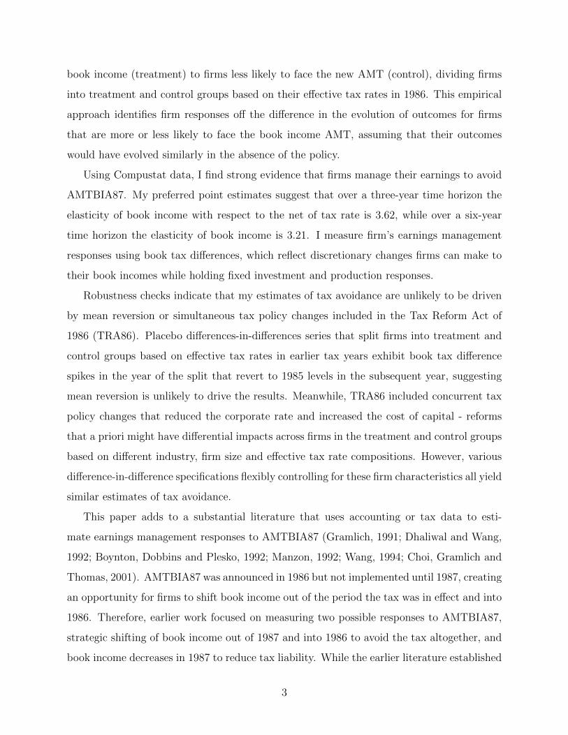
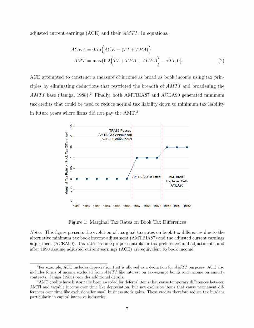
Figure 1: Marginal Tax Rates on Book Tax Differences

Notes: This figure presents the evolution of marginal tax rates on book tax differences due to thealternative minimum tax book income adjustment (AMTBIA87) and the adjusted current earningsadjustment (ACEA90). Tax rates assume proper controls for tax preferences and adjustments, andafter 1990 assume adjusted current earnings (ACE) are equivalent to book income.

2For example, ACE includes depreciation that is allowed as a deduction for AMTI purposes. ACE alsoincludes forms of income excluded from AMTI like interest on tax-exempt bonds and income on annuitycontracts. Janiga (1988) provides additional details.

3AMT credits have historically been awarded for deferral items that cause temporary differences betweenAMTI and taxable income over time like depreciation, but not exclusion items that cause permanent dif-ferences over time like exclusions for small business stock gains. These credits therefore reduce tax burdensparticularly in capital intensive industries.

7

After controlling for TPA and assuming ACE is equivalent to book income, both AMT-

BIA87 and ACEA90 imposed marginal taxes on book tax differences. I summarize variation

in the marginal tax rate on book tax differences over time in Figure 1. There was no tax on

book tax differences before 1987. From 1987-1989 AMTBIA87 imposed a 10% marginal tax

rate on book tax differences. Starting in 1990, the replacement of AMTBIA87 with ACEA90

increased the marginal tax rate on book tax differences to 15%.

2 Data

To evaluate how firms respond to AMTBIA87, I construct a balanced panel of large, per-

sistent Compustat firms that were the target of AMTBIA87, and are also likely to be the

type of firms targeted by any contemporary book income AMTs. To construct this panel, I

restrict to firms that appear in every year from 1981-1992 with positive, non-missing assets,

sales and pretax income that are incorporated in the United States and have 1986 EBITD

over $100 million.4 I end the panel in 1992 because the Omnibus Budget Reconciliation Act

of 1993 changed the ACEA90 tax base.5

Table 1 provides summary statistics for a 1985 cross section of my sample, with all

variables rescaled into 2018 dollars.6 Means far exceed medians for most variables across the

whole sample, reflecting the skewed firm size distribution. The sample only includes 8% of

all firms in Compustat in 1985, but these firms hold 32% of all assets and take in 33% of all

revenues. While these firms are not representitive of the economy as a whole, they reflect

the set of firms targeted by AMTs.

They key variable I use to categorize firms into treatment and control groups is the effec-

tive tax rate, because firms with lower effective tax rates are more likely to face AMTBIA87.

I measure effective tax rates as tax liability divided by book income, following Collins and

Shackleford (2004) to define tax liability as total income taxes minus deferred income taxes

4I calculate earnings before interest, taxes, and depreciation as income before extraordinary items plusextraordinary items and discontinued operations plus interest expense plus taxes plus depreciation andamortization.

5OBRA eliminated the adjusted current earnings depreciation adjustment for property placed in serviceafter 1993, effectively narrowing ACE by allowing depreciation deductions.

6I inflate to 2018 dollars using the GDP price deflator from NIPA table 1.1.9, “Implicit Price Deflatorsfor Gross Domestic Product” from the BEA.

8

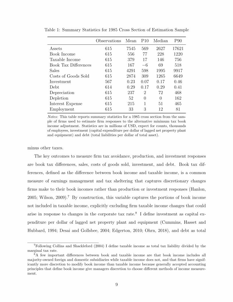
Table 1: Summary Statistics for 1985 Cross Section of Estimation Sample

Observations Mean P10 Median P90

Assets 615 7545 569 2627 17621Book Income 615 556 77 228 1220Taxable Income 615 379 17 146 756Book Tax Differences 615 167 −6 69 518Sales 615 4291 598 1995 9917Costs of Goods Sold 615 2874 309 1265 6649Investment 567 0.23 0.07 0.17 0.46Debt 614 0.29 0.17 0.29 0.41Depreciation 615 237 2 72 468Depletion 615 52 0 0 162Interest Expense 615 215 1 51 465Employment 615 33 3 12 81

Notes: This table reports summary statistics for a 1985 cross section from the sam-ple of firms used to estimate firm responses to the alternative minimum tax bookincome adjustment. Statistics are in millions of USD, expect for counts, thousandsof employees, investment (capital expenditure per dollar of lagged net property plantand equipment) and debt (total liabilities per dollar of total asset).

minus other taxes.

The key outcomes to measure firm tax avoidance, production, and investment responses

are book tax differences, sales, costs of goods sold, investment, and debt. Book tax dif-

ferences, defined as the difference between book income and taxable income, is a common

measure of earnings management and tax sheltering that captures discretionary changes

firms make to their book incomes rather than production or investment responses (Hanlon,

2005; Wilson, 2009).7 By construction, this variable captures the portions of book income

not included in taxable income, explicitly excluding firm taxable income changes that could

arise in response to changes in the corporate tax rate.8 I define investment as capital ex-

penditure per dollar of lagged net property plant and equipment (Cummins, Hasset and

Hubbard, 1994; Desai and Gollsbee, 2004; Edgerton, 2010; Ohrn, 2018), and debt as total

7Following Collins and Shackleford (2004) I define taxable income as total tax liability divided by themarginal tax rate.

8A few important differences between book and taxable income are that book income includes allmajority-owned foreign and domestic subsidiaries while taxable income does not, and that firms have signif-icantly more discretion to modify book income than taxable income because generally accepted accountingprinciples that define book income give managers discretion to choose different methods of income measure-ment.

9

liabilities per dollar of lagged assets (Edgerton, 2010; Ohrn, 2018). A substantial fraction

of finance firms in the sample are missing information required to construct the investment

variable. I also winsorize all outcome variables at the 1st and 99th percentile.

3 Empirical Strategy

AMTBIA87 was more likely to apply to firms with lower effective tax rates that report

fewer taxes paid on their financial statements. Building on previous analyses of AMTBIA87

(Dhaliwal and Wang, 1992), I assess firm responses to the policy by comparing two groups of

firms, a treatment and control group, that are more and less likely to be subject to the AMT

based on their effective tax rate (ETR).9 I compare firms with ETRs < 23% (treatment)

to firms with ETRs ≥ 23% (control) in 1986. The 23% ETR cutoff represents the ETR at

which firms are likely to no longer have to pay alternative minimum tax. I discuss the details

of this calculation in Appendix A. To execute the comparison between my treatment and

control groups, I estimate

Yit =1992∑

τ=1981,τ 6=1985

(βτ · Treatiτ

)+ β1Xit + β2Treati ·Xit + δt + γi + εit, (3)

where Treati is an indicator equal to 1 if ETR < 23% in 1986 and 0 if ETR ≥ 23% in 1986.

Treatiτ is the interaction of Treati and a year indicator (year = τ), Xit are time varying

firm-level covariates, δt are year fixed effects, and γi are firm fixed effects.

I can interpret the βτ coefficients in equation (3) as the causal impacts of AMTBIA87

on outcome variables under the assumption that the outcome variables in the treatment and

control group would have evolved similarly in the absence of the policy. However, I also relax

this assumption to allow for linear pre-trends10 by estimating

Yit = α · Treati · t+1992∑

τ=1986

(βτ · Treatiτ

)+ β1Xit + β2Treati ·Xit + δt + γi + εit. (4)

In equation (4), the βτ coefficients can be interpreted as the causal effect of AMTBIA87 on

9I measure effective tax rates as tax liability divided by book income in each year.10For another example of this approach, see Dobkin, Finklestein, Kluender and Notowidigdo (2018).

10

firm’s outcomes under the assumption that any linear outcome trend for treatment relative

to control firms in the pre-period would have continued in the absence of AMTBIA87.

Equations (3) and (4) estimate firm responses to AMTBIA87 using a binary treatment

approach, identifying the average treatment effect of the policy before and after allowing for

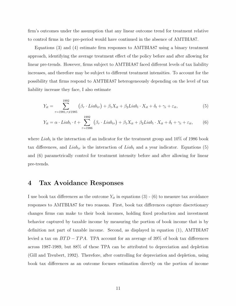
linear pre-trends. However, firms subject to AMTBIA87 faced different levels of tax liability

increases, and therefore may be subject to different treatment intensities. To account for the

possibility that firms respond to AMTBIA87 heterogeneously depending on the level of tax

liability increase they face, I also estimate

Yit =1992∑

τ=1981,τ 6=1985

(βτ · Liabiτ

)+ β1Xit + β2Liabi ·Xit + δt + γi + εit, (5)

Yit = α · Liabi · t+1992∑

τ=1986

(βτ · Liabiτ

)+ β1Xit + β2Liabi ·Xit + δt + γi + εit, (6)

where Liabi is the interaction of an indicator for the treatment group and 10% of 1986 book

tax differences, and Liabiτ is the interaction of Liabi and a year indicator. Equations (5)

and (6) parametrically control for treatment intensity before and after allowing for linear

pre-trends.

4 Tax Avoidance Responses

I use book tax differences as the outcome Yit in equations (3) - (6) to measure tax avoidance

responses to AMTBIA87 for two reasons. First, book tax differences capture discretionary

changes firms can make to their book incomes, holding fixed production and investment

behavior captured by taxable income by measuring the portion of book income that is by

definition not part of taxable income. Second, as displayed in equation (1), AMTBIA87

levied a tax on BTD − TPA. TPA account for an average of 39% of book tax differences

across 1987-1989, but 88% of these TPA can be attributed to depreciation and depletion

(Gill and Treubert, 1992). Therefore, after controlling for depreciation and depletion, using

book tax differences as an outcome focuses estimation directly on the portion of income

11

taxed by AMTBIA87 without capturing taxable income responses.11

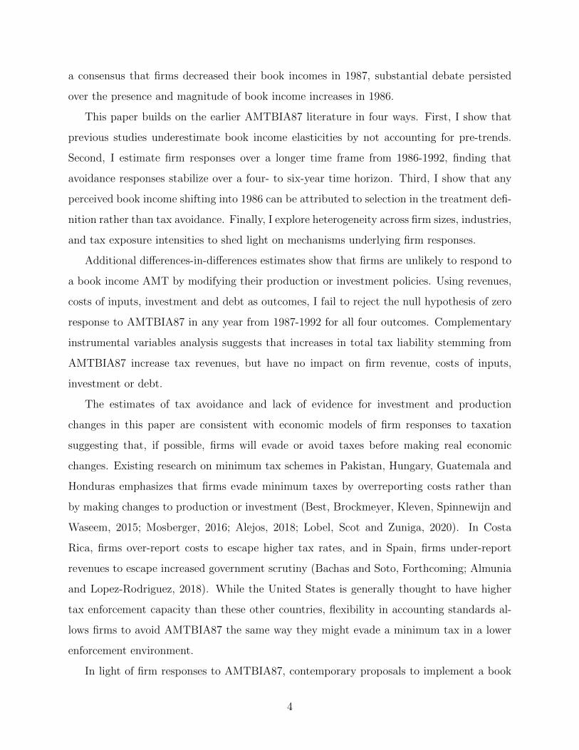
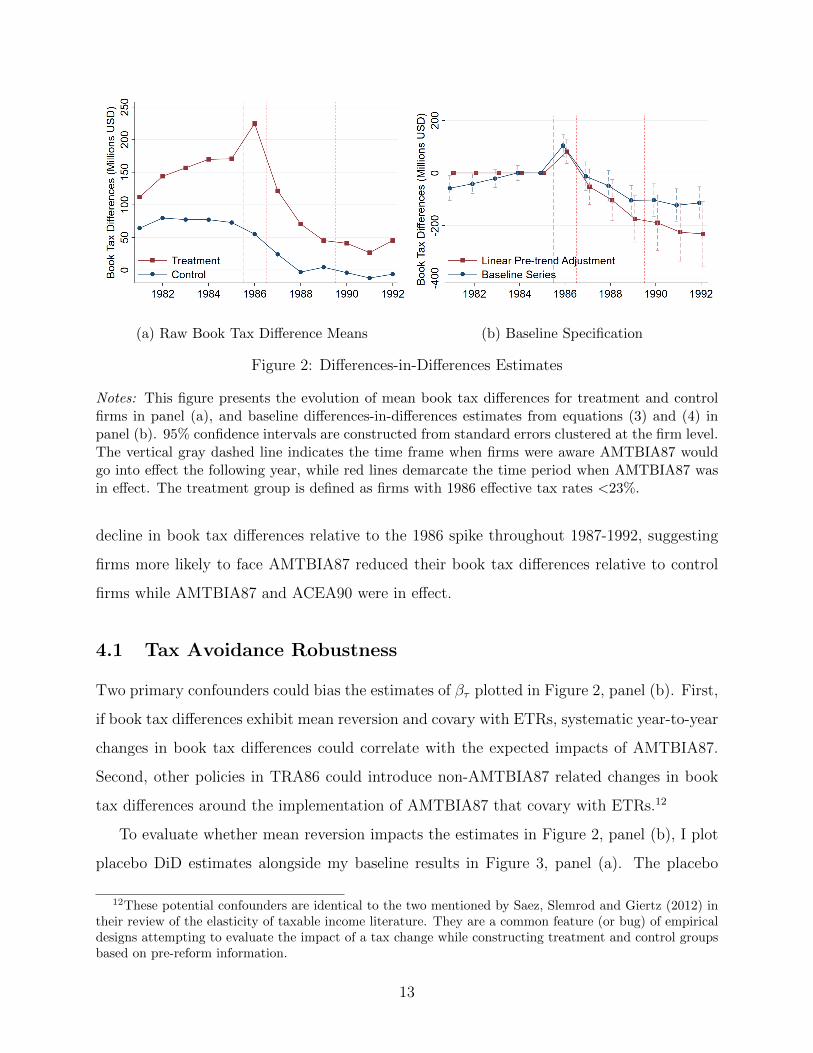
To portray the raw data over time, Figure 2, panel (a) plots the progression of book tax

difference means by year for treatment and control firms. Three important points arise from

panel (a). First, book tax differences appear to increase for treatment relative to control firms

in the pre-period. Second, treatment firms exhibit a sharp increase in book tax differences

in 1986, providing suggestive evidence that firms responded to AMTBIA87 by shifting book

income into 1986. Finally, book tax differences decline for treatment firms relative to control

firms in the periods while AMTBIA87 and ACEA90 are in effect.

Formalizing the comparison of raw means in Figure 2, panel (a), I plot the βτ coefficients

from equation (3) bracketed by their 95% confidence intervals in the baseline series of Figure

2, panel (b). Standard errors are clustered at the firm level. I include firm assets, sales,

interest expense, depreciation, depletion and number of employees in Xit to control for

changes in firm size, the possibility that tax incentives differentially impact firms with low

versus high ETRs, and the vast majority of tax preferences and adjustments to isolate

variation in the outcome independent of non-AMTBIA87 tax incentives.

The baseline series in panel (b) exhibits clear pre-trends, suggesting that estimates of

equation (3) are likely to understate firm tax avoidance in response to AMTBIA87. Guided

by the data, I also estimate equation (4) and plot the βτ coefficients in the pre-trend ad-

justment series of panel (b). This pre-trend correction is conservative in the sense that if it

overstates firm responses to AMTBIA87, I will understate the revenue a book income AMT

would raise in the scoring exercise in section 6.

The pre-trend adjustment series displays two important results. First, there appears

to be a clear increase in book tax differences in 1986 for firms more likely to be subject

to AMTBIA87 the next year, suggesting firms more likely to face AMTBIA87 strategically

concentrated book income independent of taxable income into 1986 before book income was

subject to a tax. Second, firms more likely to be subject to AMTBIA87 exhibit a clear

11With administrative tax data, I could simply subtract TPA from the outcome. However, depreciationand depletion in Compustat do not exactly measure the depreciation and depletion components of TPA. Forexample, TPA includes depreciation of property placed in service after 1986, not all depreciation. Therefore,controlling for variation in Compustat depreciation over time captures changes to depreciation included inTPA without introducing substantial measurement error in the outcome based on previous depreciationlevels which are likely to covary with treatment status.

12

(a) Raw Book Tax Difference Means (b) Baseline Specification

Figure 2: Differences-in-Differences Estimates

Notes: This figure presents the evolution of mean book tax differences for treatment and controlfirms in panel (a), and baseline differences-in-differences estimates from equations (3) and (4) inpanel (b). 95% confidence intervals are constructed from standard errors clustered at the firm level.The vertical gray dashed line indicates the time frame when firms were aware AMTBIA87 wouldgo into effect the following year, while red lines demarcate the time period when AMTBIA87 wasin effect. The treatment group is defined as firms with 1986 effective tax rates <23%.

decline in book tax differences relative to the 1986 spike throughout 1987-1992, suggesting

firms more likely to face AMTBIA87 reduced their book tax differences relative to control

firms while AMTBIA87 and ACEA90 were in effect.

4.1 Tax Avoidance Robustness

Two primary confounders could bias the estimates of βτ plotted in Figure 2, panel (b). First,

if book tax differences exhibit mean reversion and covary with ETRs, systematic year-to-year

changes in book tax differences could correlate with the expected impacts of AMTBIA87.

Second, other policies in TRA86 could introduce non-AMTBIA87 related changes in book

tax differences around the implementation of AMTBIA87 that covary with ETRs.12

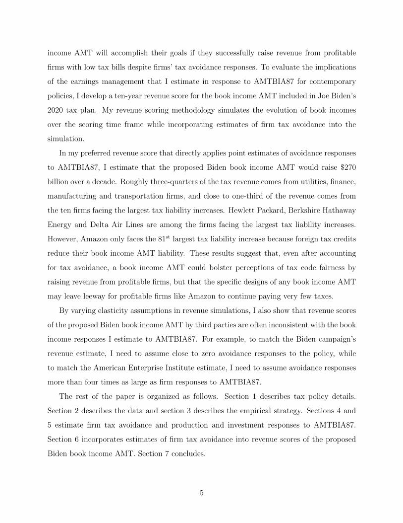
To evaluate whether mean reversion impacts the estimates in Figure 2, panel (b), I plot

placebo DiD estimates alongside my baseline results in Figure 3, panel (a). The placebo

12These potential confounders are identical to the two mentioned by Saez, Slemrod and Giertz (2012) intheir review of the elasticity of taxable income literature. They are a common feature (or bug) of empiricaldesigns attempting to evaluate the impact of a tax change while constructing treatment and control groupsbased on pre-reform information.

13

series exactly replicate the baseline estimates of equation (3) in Figure 2, panel (b), but

define treatment and control groups based on ETRs in 1982, 1983, 1984 and 1985 rather

than 1986. These placebo series make two important points. First, placebos exhibit book tax

difference declines similar to the baseline series, but the declines diminish in magnitude for

the earlier treatment control splits. This pattern is consistent with the estimated treatment

effects representing firm responses to AMTBIA87, where splitting into treatment and control

firms in earlier years captures fewer firms likely to be subject to AMTBIA87.

Second, despite no policy incentive to do so, treatment firms exhibit a spike in book tax

differences in the year I split firms into treatment and control groups based on ETRs that

diminishes in the following year or two. Therefore, selection of high book tax difference firms

for the treatment group appears to bias β86 upward, while mean reversion does not appear

to have a significant impact on my estimates because book tax differences largely revert in

the year after the treatment designation.

The finding that a significant portion of the 1986 book tax difference spike can be at-

tributed to selection rather than a real avoidance response clarifies the lack of consensus

over firm responses in 1986 in the existing literature.13 The placebo series in Figure 3, panel

(a) make clear that this disagreement stems from different treatment and control definitions

across studies, not real avoidance responses. To formally test that the observed 1986 spike

is not a real avoidance response I stack the 1982-1985 placebo series and estimate an event

study defining event-time zero to be the year I split each placebo series into treatment and

control groups. The event-time zero coefficient in this specification aggregates observed book

tax difference spikes in the year I split into treatment and control groups, effectively aver-

aging over the spikes in each placebo series. A Wald test for the equality of the event-time

zero estimate and the 1986 coefficient from equation (4) fails to reject the null hypothesis at

the 10% level.14

13Gramlich (1991); Dhaliwal and Wang (1992); Wang (1994) all find evidence that firms shift largeamounts of book income into 1986 to avoid AMTBIA87, while Boynton, Dobbins and Plesko (1992); Choi,Gramlich and Thomas (2001) find no evidence of this behavior.

14I append versions of my estimation sample with treatment groups defined in each placebo year, defineevent time relative to treatment-control split as k, and estimate BTDik =

∑10k=−4 βkTreatik + β1Xik +

β2Xik ·Treati + δt + γi + νik. I then test H0 : βk=0 = β86 where β86 comes from equation (4). An analogoustest using the baseline series without the pre-trend adjustment fails to reject the null of equal coefficients atthe 5% level.

14

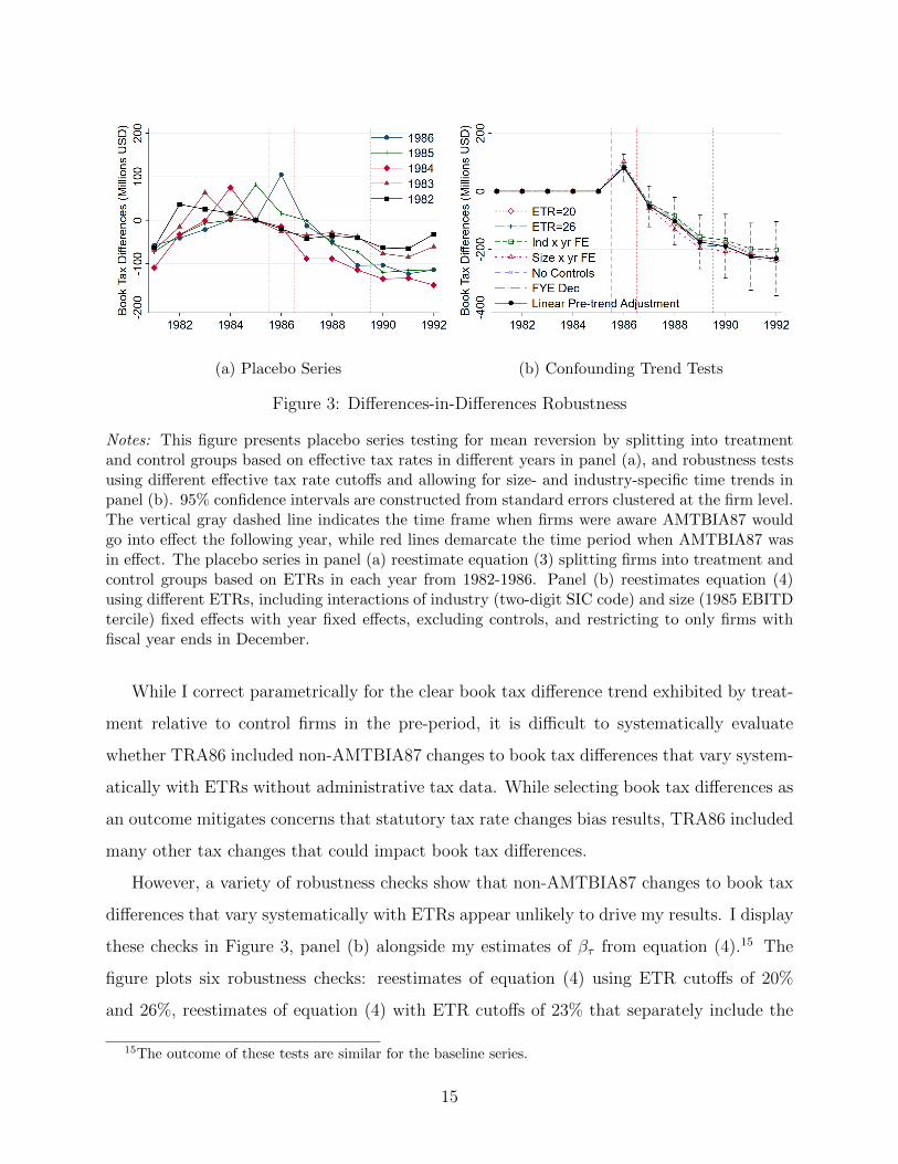
(a) Placebo Series (b) Confounding Trend Tests

Figure 3: Differences-in-Differences Robustness

Notes: This figure presents placebo series testing for mean reversion by splitting into treatmentand control groups based on effective tax rates in different years in panel (a), and robustness testsusing different effective tax rate cutoffs and allowing for size- and industry-specific time trends inpanel (b). 95% confidence intervals are constructed from standard errors clustered at the firm level.The vertical gray dashed line indicates the time frame when firms were aware AMTBIA87 wouldgo into effect the following year, while red lines demarcate the time period when AMTBIA87 wasin effect. The placebo series in panel (a) reestimate equation (3) splitting firms into treatment andcontrol groups based on ETRs in each year from 1982-1986. Panel (b) reestimates equation (4)using different ETRs, including interactions of industry (two-digit SIC code) and size (1985 EBITDtercile) fixed effects with year fixed effects, excluding controls, and restricting to only firms withfiscal year ends in December.

While I correct parametrically for the clear book tax difference trend exhibited by treat-

ment relative to control firms in the pre-period, it is difficult to systematically evaluate

whether TRA86 included non-AMTBIA87 changes to book tax differences that vary system-

atically with ETRs without administrative tax data. While selecting book tax differences as

an outcome mitigates concerns that statutory tax rate changes bias results, TRA86 included

many other tax changes that could impact book tax differences.

However, a variety of robustness checks show that non-AMTBIA87 changes to book tax

differences that vary systematically with ETRs appear unlikely to drive my results. I display

these checks in Figure 3, panel (b) alongside my estimates of βτ from equation (4).15 The

figure plots six robustness checks: reestimates of equation (4) using ETR cutoffs of 20%

and 26%, reestimates of equation (4) with ETR cutoffs of 23% that separately include the

15The outcome of these tests are similar for the baseline series.

15

interaction of size (1985 EBITD tercile) and year fixed effects, and industry (two-digit SIC

code)16 and year fixed effects, and reestimates of equation (4) without controls and restricting

to only firms with fiscal year-ends in December. Estimates are remarkably similar across

these specifications. In every case, book tax difference responses of treatment relative to

control firms exhibit a near-identical pattern. Therefore, if bias of the magnitude necessary

to cast doubt on my baseline estimates exists, the bias cannot depend explicitly on the

ETR cutoff, cannot be driven by any industry specific or firm-size specific time trends, is

not driven by the inclusion or exclusion of controls, and is not specific to firms with fiscal

year-ends not in December.

4.2 Scaling Tax Avoidance Responses

Figure 2, panel (b) displays average treatment effects of AMTBIA87 over different time hori-

zons for my entire sample. To better understand whether these estimates are quantitatively

large, I scale these average treatment effects in two ways. First, I estimate the continuous

DiD specifications from equations (5) and (6) to identify the book tax difference response

of treatment firms per dollar of expected new tax liability due to AMTBIA87. Second, I

rescale the βτ coefficients into an elasticity to quantify the scale of tax avoidance responses

relative to firm book incomes and marginal tax rate changes.

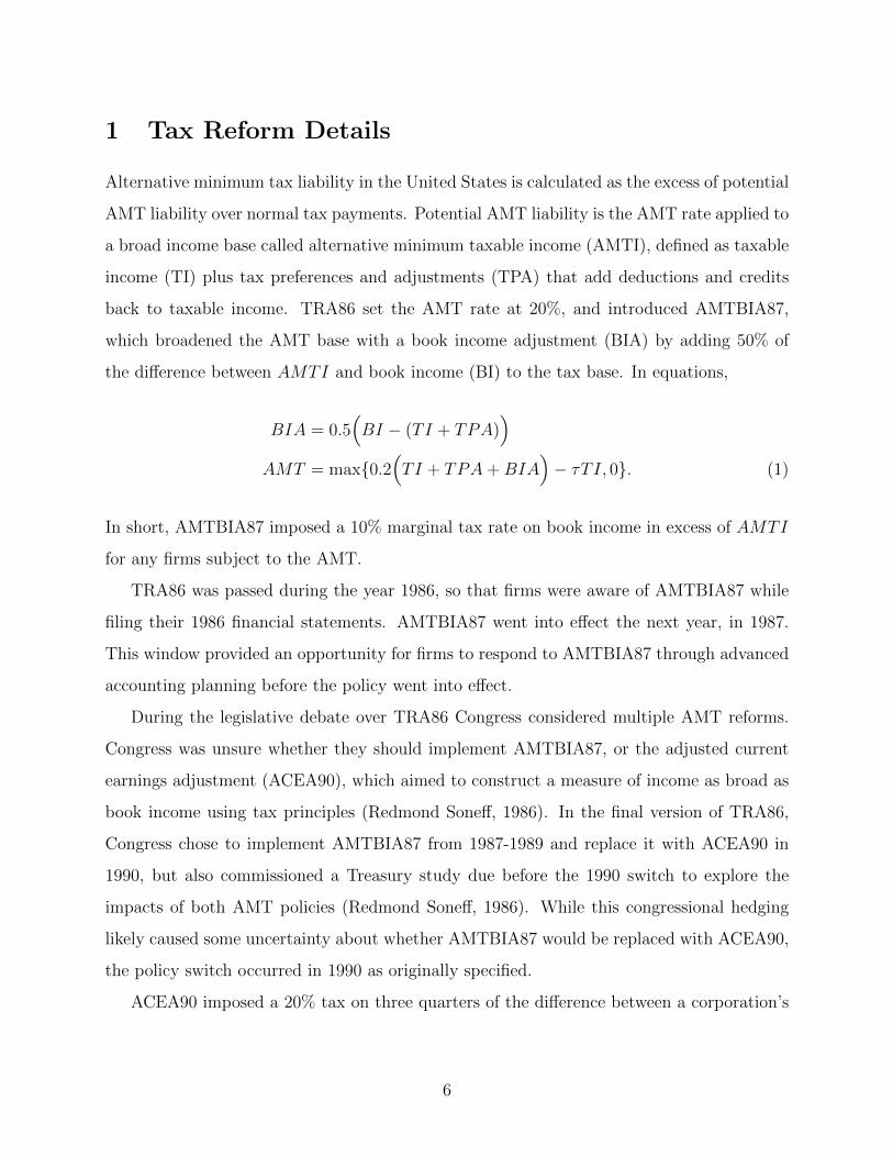
Figure 4 displays firm tax avoidance responses to AMTBIA87 accounting for different

treatment intensities. I measure treatment intensity as the expected tax liability under

AMTBIA87 based on 1986 book incomes, calculating Liabi as the interaction of a treatment

dummy with 10% of 1986 book tax differences. Panel (a) plots three series that reestimate

equation (4), partitioning the treatment group into low, medium and high intensity groups

by Liabi terciles and only including a single tercile of the treatment group in each series. The

series show that firms have larger tax avoidance responses to AMTBIA87 if they face more

tax liability. To parametrically quantify the impact of each additional dollar of expected

AMTBIA87 tax liability on tax avoidance, I plot the βτ coefficients from equations (5) and

16To standardize SIC codes within firms I use the mode SIC code within firms across years, breaking tiesarbitrarily with the smaller SIC code. I impute two digit SIC codes manually based on financial statementinformation for firms missing an SIC code in every year.

16

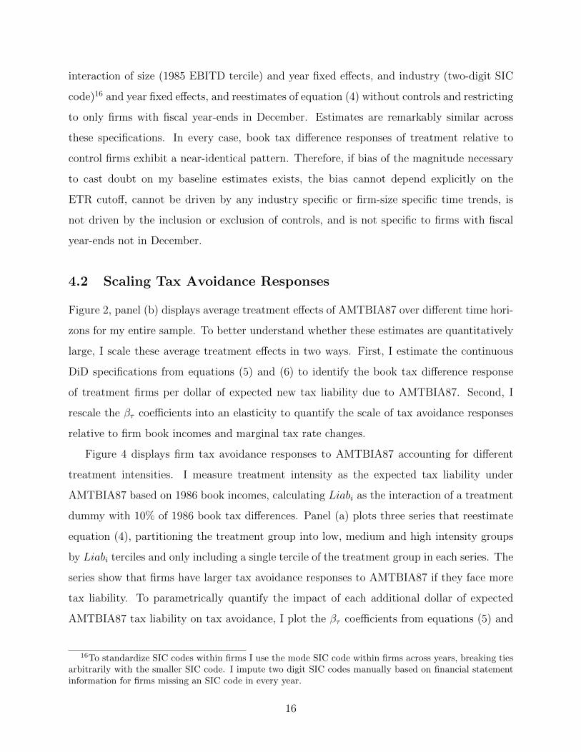
(a) Coarse Treatment Intensity (b) Parametric Treatment Intensity

Figure 4: Differences-in-Differences Estimates by Treatment Intensity

Notes: This figure plots estimates of tax avoidance in response to the alternative minimum tax bookincome adjustment accounting for heterogeneous treatment intensities. Panel (a) plots estimates ofβτ from equation (4), partitioning the treatment group into low, medium and high intensity groupsby Liabi terciles and only including a single tercile of the treatment group in each series. Panel (b)plots estimates of βτ from equations (5) and (6) in the baseline and linear pre-trend adjustmentseries respectively.

(6) in the baseline and linear pre-trend adjustment series in panel (b). The linear pre-trend

adjustment series indicates that for every additional expected $1 million of AMTBIA87 tax

liability firms reduce their book tax differences by approximately $8 million in 1989.

To quantify the magnitude of my estimates relative to firm’s book incomes and marginal

tax changes, I express my estimates of tax avoidance in response to AMTBIA87 in terms of

the elasticity of book income with respect to the net of tax rate, defined as

εBIt =∆BTDt

∆(1− τ)t· 1− τBI85

, (7)

where τ is the tax rate on book income, BTD are book tax differences, BI is book income,

and t is the year. This elasticity can be interpreted as the percent change in book income

in year t (measured via book tax differences to capture tax avoidance responses) when the

net of tax rate increases by 1%. As displayed in Figure 1, τ is zero before 1987, increases to

0.1 for 1987-1989, and increases again to 0.15 in 1990.

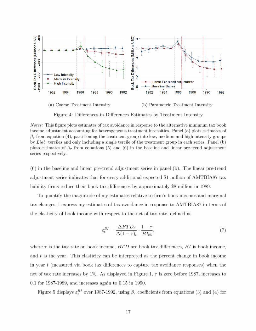
Figure 5 displays εBIt over 1987-1992, using βτ coefficients from equations (3) and (4) for

17

Figure 5: Book Income Elasticities

Notes: This figure plots εBIt , the elasticity of book income with respect to the net of tax rate,with 95% confidence intervals constructed from non-parametrically bootstrapped standard errorsclustering at the firm level. εBIt = ∆BTDt

∆(1−τ)t· 1−τBI85

, where ∆BTDt are the differences-in-differences

estimates of firm responses to AMTBIA87 displayed in Figure 2, panel (b).

∆BTDt, constructing confidence intervals from non-parametrically bootstrapped standard

errors clustering at the firm level to account for uncertainty in both average book income in

1985 and the DiD estimates of book income responses. Using my preferred estimates from

the linear pre-trend adjusted series, the elasticity of book income peaks at 3.62 in 1989 and

stabilizes around 3.21 by 1992. This figure makes clear that earlier studies underestimate

book income elasticities by not correcting for pre-trends. Dharmapala (2020) aggregates

estimates of the elasticity of book income, finding that results in Dhaliwal and Wang (1992)

imply a book income elasticity of 1.7, while results in Manzon (1992) imply a range of elas-

ticities from 1.4-2.1. Both estimates are directly in line with my estimates before correcting

for pre-trends, but are lower than estimates after correcting for pre-trends.

4.3 Tax Avoidance Heterogeneity

The elasticities in the linear pre-trend adjusted series in Figure 5 represent my preferred

estimates of the average book income responses of treatment firms relative to control firms.

18

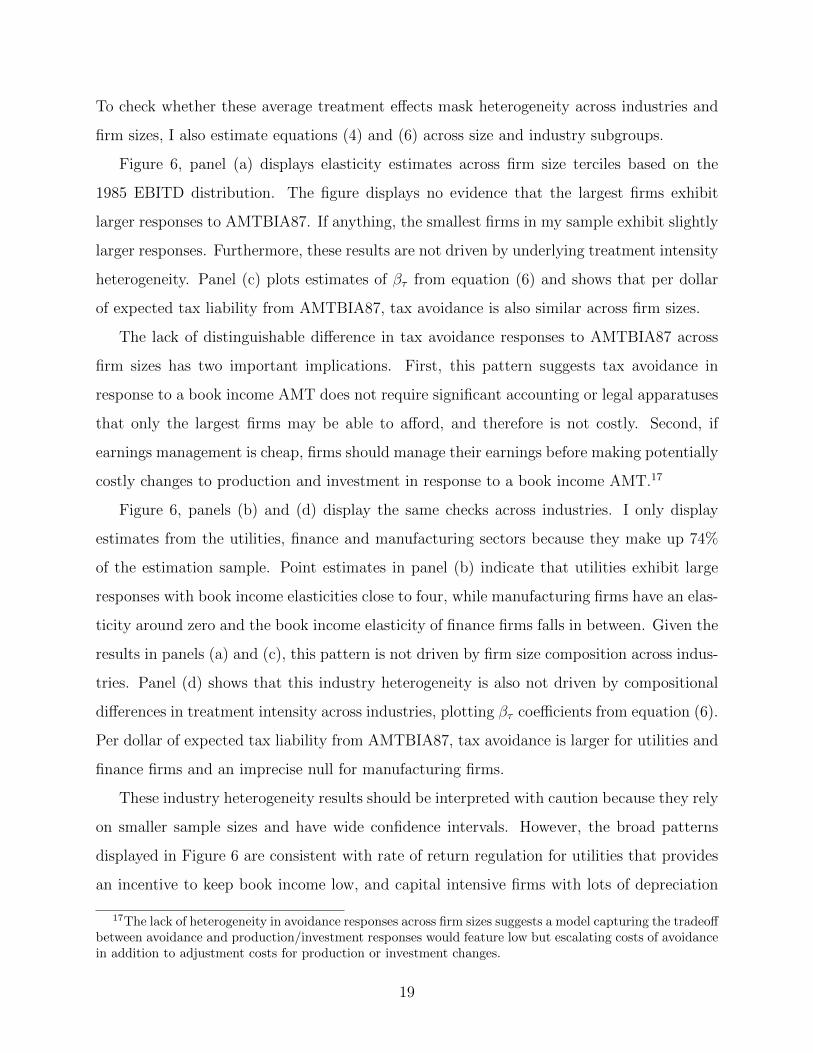
To check whether these average treatment effects mask heterogeneity across industries and

firm sizes, I also estimate equations (4) and (6) across size and industry subgroups.

Figure 6, panel (a) displays elasticity estimates across firm size terciles based on the

1985 EBITD distribution. The figure displays no evidence that the largest firms exhibit

larger responses to AMTBIA87. If anything, the smallest firms in my sample exhibit slightly

larger responses. Furthermore, these results are not driven by underlying treatment intensity

heterogeneity. Panel (c) plots estimates of βτ from equation (6) and shows that per dollar

of expected tax liability from AMTBIA87, tax avoidance is also similar across firm sizes.

The lack of distinguishable difference in tax avoidance responses to AMTBIA87 across

firm sizes has two important implications. First, this pattern suggests tax avoidance in

response to a book income AMT does not require significant accounting or legal apparatuses

that only the largest firms may be able to afford, and therefore is not costly. Second, if

earnings management is cheap, firms should manage their earnings before making potentially

costly changes to production and investment in response to a book income AMT.17

Figure 6, panels (b) and (d) display the same checks across industries. I only display

estimates from the utilities, finance and manufacturing sectors because they make up 74%

of the estimation sample. Point estimates in panel (b) indicate that utilities exhibit large

responses with book income elasticities close to four, while manufacturing firms have an elas-

ticity around zero and the book income elasticity of finance firms falls in between. Given the

results in panels (a) and (c), this pattern is not driven by firm size composition across indus-

tries. Panel (d) shows that this industry heterogeneity is also not driven by compositional

differences in treatment intensity across industries, plotting βτ coefficients from equation (6).

Per dollar of expected tax liability from AMTBIA87, tax avoidance is larger for utilities and

finance firms and an imprecise null for manufacturing firms.

These industry heterogeneity results should be interpreted with caution because they rely

on smaller sample sizes and have wide confidence intervals. However, the broad patterns

displayed in Figure 6 are consistent with rate of return regulation for utilities that provides

an incentive to keep book income low, and capital intensive firms with lots of depreciation

17The lack of heterogeneity in avoidance responses across firm sizes suggests a model capturing the tradeoffbetween avoidance and production/investment responses would feature low but escalating costs of avoidancein addition to adjustment costs for production or investment changes.

19

(a) Elasticities by Size (b) Elasticities by Industry

(c) Parametric Treatment Intensity by Size (d) Parametric Treatment Intensity by Industry

Figure 6: Size and Industry Tax Avoidance Heterogeneity

Notes: This figure plots tax avoidance responses to AMTBIA87 across firm sizes and industries.Panels (a) and (b) plot εBIt , the elasticity of book income with respect to the net of tax rate,with 95% confidence intervals constructed from non-parametrically bootstrapped standard errorsclustering at the firm level. εBIt = ∆BTDt

∆(1−τ)t· 1−τBI85

, where ∆BTDt are the differences-in-differences

estimates of firm responses to AMTBIA87 across 1985 EBITD terciles in panel (a) and industriesin panel (b). Panels (c) and (d) display estimates of βτ from equation (6) across 1985 EBITDterciles and industries. Industries include manufacturing (SIC codes 2000-3999), utilities (SICcodes 4900-4999) and finance and insurance (SIC codes 4000-4899).

having less scope to manage earnings because a large fraction of their book tax differences

come from the different depreciation schedules mandated by GAAP and tax rules.

AMT credits do not appear to play a significant role in firm tax avoidance responses to

AMTBIA87. Firms were awarded AMT credits for preferences that caused temporary differ-

ences between taxable income and alternative minimum taxable income like depreciation, but

20

not “exclusion items” that caused permanent differences like depletion. However, in 1990,

depletion became eligible to generate AMT credits (Gerardi, Milner and Silverstein, 1992).

Utility firms have high depletion, and treatment utility firms have higher depletion than

control utility firms. Therefore, if AMT credits played a significant role in firm responses

we would expect estimated avoidance responses for utility firms to decline in 1990-1992.18

Instead, we see no decline in utility firm’s tax avoidance from 1990-1992 in Figure 6, panel

(b). This is not surprising in light of existing evidence that firms respond to tax policy when

it impacts immediate but not future cash flows (Zwick and Mahon, 2017).

4.4 Tax Avoidance Responses to Policy Transition

One final concern about the estimates of tax avoidance throughout this section is that the

interpretation of post-1989 coefficients is complicated by the replacement of AMTBIA87

with the adjusted current earnings adjustment (ACEA90) in 1990. Until this point, I have

assumed the marginal tax rates displayed in Figure 1 are correct, or that adjusted current

earnings (ACE) are equivalent to book income. However, this assumption is not exactly

correct because ACE are based on tax principles, not accounting rules.

There are two different ways to view estimates of firm tax avoidance responses in 1990-

1992. In the first view, ACEA90 taxes the same base as AMTBIA87 at a higher 15%

marginal tax rate. In the second view, ACEA90 taxes a different base than AMTBIA87 at a

higher rate, so that the elasticities calculated in accordance with the first view conflate firm

responses to a tax on book income in excess of alternative minimum taxable income (AMTI)

with a tax on a different base. To distinguish between these two alternative interpretations of

elasticities over a four- to six-year horizon, I test whether firms respond to the transition from

AMTBIA87 to ACEA90. A clear book tax difference decline in response to the transition

would indicate firms face a higher tax rate on a similar tax base. On the other hand, no firm

response to the transition would suggest firms do not face a higher tax rate on the same tax

base, and that I subsequently underestimate elasticities over a four- to six-year horizon.

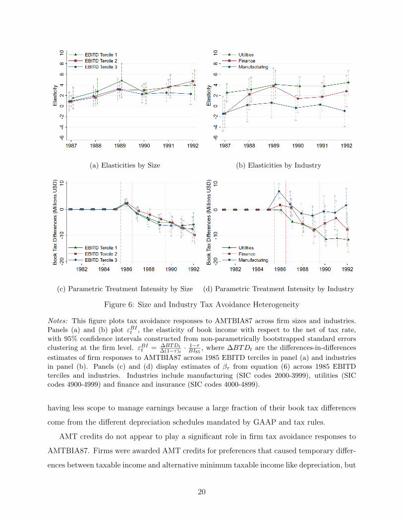
To execute this test, I reestimate equation (3) on a panel of Compustat firms that appear

18These differences would not be captured by the depletion controls in equations (3) - (6) because thesecontrols assume the impact of depletion on book tax differences is fixed over time.

21

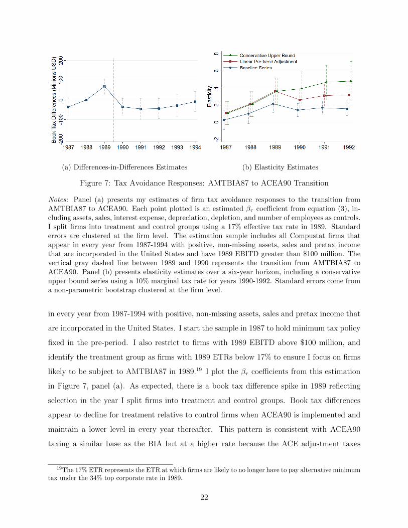
(a) Differences-in-Differences Estimates (b) Elasticity Estimates

Figure 7: Tax Avoidance Responses: AMTBIA87 to ACEA90 Transition

Notes: Panel (a) presents my estimates of firm tax avoidance responses to the transition fromAMTBIA87 to ACEA90. Each point plotted is an estimated βτ coefficient from equation (3), in-cluding assets, sales, interest expense, depreciation, depletion, and number of employees as controls.I split firms into treatment and control groups using a 17% effective tax rate in 1989. Standarderrors are clustered at the firm level. The estimation sample includes all Compustat firms thatappear in every year from 1987-1994 with positive, non-missing assets, sales and pretax incomethat are incorporated in the United States and have 1989 EBITD greater than $100 million. Thevertical gray dashed line between 1989 and 1990 represents the transition from AMTBIA87 toACEA90. Panel (b) presents elasticity estimates over a six-year horizon, including a conservativeupper bound series using a 10% marginal tax rate for years 1990-1992. Standard errors come froma non-parametric bootstrap clustered at the firm level.

in every year from 1987-1994 with positive, non-missing assets, sales and pretax income that

are incorporated in the United States. I start the sample in 1987 to hold minimum tax policy

fixed in the pre-period. I also restrict to firms with 1989 EBITD above $100 million, and

identify the treatment group as firms with 1989 ETRs below 17% to ensure I focus on firms

likely to be subject to AMTBIA87 in 1989.19 I plot the βτ coefficients from this estimation

in Figure 7, panel (a). As expected, there is a book tax difference spike in 1989 reflecting

selection in the year I split firms into treatment and control groups. Book tax differences

appear to decline for treatment relative to control firms when ACEA90 is implemented and

maintain a lower level in every year thereafter. This pattern is consistent with ACEA90

taxing a similar base as the BIA but at a higher rate because the ACE adjustment taxes

19The 17% ETR represents the ETR at which firms are likely to no longer have to pay alternative minimumtax under the 34% top corporate rate in 1989.

22

three quarters rather than half the gap between a broader income measure and AMTI.

However, interpretation of the post-1989 coefficients is difficult for two reasons. First,

all of the post-1989 coefficients do not reject the null hypothesis of zero at the 5% level.

Second, the post-1989 coefficients may be biased upwards if there is a pre-trend. While

the 1987 coefficient indicates this may be the case, I view two pre-treatment periods as

insufficient to estimate any reliable pre-trend correction.20

In summary, Figure 7 suggests that firms exhibit responses to the transition from AMT-

BIA87 to ACEA90 so that applying a 15% marginal tax rate change over a four- to six-year

horizon in elasticity calculations is reasonable. Unfortunately, this evidence is not defini-

tive. To account for this uncertainty conservatively, I calculate upper bounds on elasticities

over a four- to six-year time horizon using a 10% marginal tax rate change in those years

to proxy for ACEA90 applying a higher rate to a narrower base. This calculation yields

{εBIt }t=90,91,92 = {3.93,4.67,4.81}. I plot this elasticity series in Figure 7, panel (b).

5 Production and Investment Responses

Firms have some freedom to manage their earnings to avoid AMTBIA87, but face adjustment

costs if they want to make production and investment policy changes (Doms and Dunne,

1998; Cooper and Haltiwanger, 2006), suggesting that firms should avoid AMTBIA87 but

not respond by making changes to production or investment. The lack of heterogeneity in

tax avoidance responses across firm sizes in section 4 reinforces this hypothesis.

To test whether firms exhibit real production and investment responses to AMTBIA87,

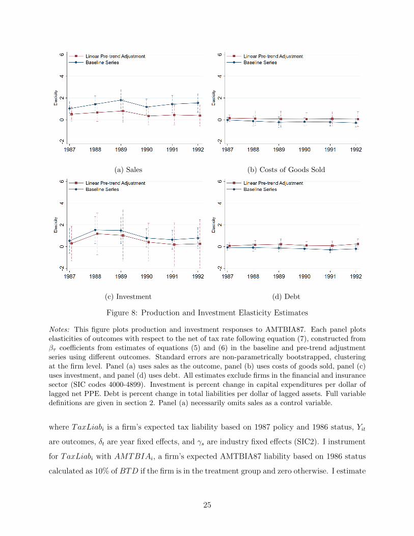
Figure 8 plots elasticity estimates analogous to those presented in Figure 5, constructed

from estimates of equations (3) and (4) using sales, costs of goods sold (COGS), investment,

and debt as outcomes.21 These elasticities can be interpreted as the percent decline in each

20A third potential bias exists for the 1990 coefficient, but is second order. This possible bias stems fromthe fact that there was a small recession in 1990, and negative book tax differences increase in magnitudeduring recessions (Gaertner, Laplante and Lynch, 2016). Treatment firms in this exercise have ex-anteresponsive book income because they maintain low ETRs even in the presence of AMTBIA87 for threeyears. Therefore, it is not unreasonable to expect the ex-ante responsive treatment group to also have largernegative book tax difference responses to the recession in 1990.

21I exclude finance firms from these estimates because capital stock and revenue variables can reflectdifferent quantities for these firms.

23

outcome variable for each 1% increase in the marginal tax rate on book tax differences

imposed by AMTBIA87.

None of the estimates from the pre-trend adjusted series can reject the null of zero in

any of the post-1986 years across all four outcomes, suggesting that firms did not exhibit

significant production and investment responses to AMTBIA87. The sales and COGS esti-

mates in panels (a) and (b) suggest that firms did not modify their production in response

to AMTBIA87 because there are no clear changes in firm revenues or costs of inputs.

Firms also do not appear to make economically meaningful changes to their investment

and debt in response to AMTBIA87. In panel (d), I reject 1989 increases in liabilities of

more than 0.26% and decreases of more than 0.71% of lagged assets for every 1% increase in

the marginal tax rate on book tax differences. In panel (c), the investment estimates yield

an imprecise null. The 1989 coefficient cannot reject capital expenditure increases of more

than 1.29% or decreases of more than 3.35% of lagged capital stock for every 1% change in

the net of tax rate on book tax differences.

The estimates in Figure 8 should be interpreted with caution because TRA86 made other

concurrent changes to tax policy that modified incentives for investment and production.

However, one reassuring feature of these estimates is that potential biases from concurrent

policy changes correspond with the signs of point estimates that diverge from zero. For

example, lowering the corporate tax rate should provide a stronger incentive for high ETR

firms in the control group to increase revenues, suggesting that the sales estimates for treat-

ment firms in panel (a) may be biased upwards. In addition, low ETR treatment firms have

low ETRs in part because they take advantage of tax incentives for investment. Raising

the cost of capital may disproportionately reduce incentives for low ETR firms with more

investment, suggesting the investment elasticities in panel (c) may also be biased upwards.

To summarize and complement the DiD production and investment responses presented in

Figure 8, I also estimate the impact of tax liability on outcomes, using expected AMTBIA87

liability as an instrument for total tax liability and estimating

Yit = φTaxLiabi + βXit + δt + γs + εit, (8)

24

(a) Sales (b) Costs of Goods Sold

(c) Investment (d) Debt

Figure 8: Production and Investment Elasticity Estimates

Notes: This figure plots production and investment responses to AMTBIA87. Each panel plotselasticities of outcomes with respect to the net of tax rate following equation (7), constructed fromβτ coefficients from estimates of equations (5) and (6) in the baseline and pre-trend adjustmentseries using different outcomes. Standard errors are non-parametrically bootstrapped, clusteringat the firm level. Panel (a) uses sales as the outcome, panel (b) uses costs of goods sold, panel (c)uses investment, and panel (d) uses debt. All estimates exclude firms in the financial and insurancesector (SIC codes 4000-4899). Investment is percent change in capital expenditures per dollar oflagged net PPE. Debt is percent change in total liabilities per dollar of lagged assets. Full variabledefinitions are given in section 2. Panel (a) necessarily omits sales as a control variable.

where TaxLiabi is a firm’s expected tax liability based on 1987 policy and 1986 status, Yit

are outcomes, δt are year fixed effects, and γs are industry fixed effects (SIC2). I instrument

for TaxLiabi with AMTBIAi, a firm’s expected AMTBIA87 liability based on 1986 status

calculated as 10% of BTD if the firm is in the treatment group and zero otherwise. I estimate

25

this regression over all treatment and controls firms after exluding the financial sector, using

all data from 1987-1992.

The two stage least squares estimates identify the causal effect of additional tax liability

on outcomes under the assumption that expected AMTBIA87 liability impacts outcomes

only through changes in tax liability. The instrument is relevant because expected AMT-

BIA87 liability is mechanically related to expected total tax liability, and unlikely to violate

exclusion unless firms respond to AMTBIA87 for reasons unrelated to tax liability changes.22

Estimates of the predicted tax liability coefficient φ are particularly useful because they

can be interpreted as the impact of tax liability on outcomes, but are identified using only

variation in expected AMTBIA87 liability. In addition, constructing the instrument from

BTD eliminates concerns that DiD controls for TPA do not rid my estimates of bias from

mismeasuring the tax base if tax base error is independent across firms.

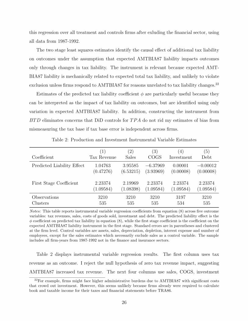
Table 2: Production and Investment Instrumental Variable Estimates

(1) (2) (3) (4) (5)Coefficient Tax Revenue Sales COGS Investment Debt

Predicted Liability Effect 1.04763 3.95585 −6.37969 0.00001 −0.00012(0.47276) (6.53215) (3.93969) (0.00008) (0.00008)

First Stage Coefficient 2.23374 2.19969 2.23374 2.23374 2.23374(1.09584) (1.08398) (1.09584) (1.09584) (1.09584)

Observations 3210 3210 3210 3197 3210Clusters 535 535 535 534 535

Notes: This table reports instrumental variable regression coefficients from equation (8) across five outcomevariables: tax revenues, sales, costs of goods sold, investment and debt. The predicted liability effect is theφ coefficient on predicted tax liability in equation (8), while the first stage coefficient is the coefficient on theexpected AMTBIA87 liability instrument in the first stage. Standard errors are in parentheses and clusteredat the firm level. Control variables are assets, sales, depreciation, depletion, interest expense and number ofemployees, except for the sales estimates which necessarily exclude sales as a control variable. The sampleincludes all firm-years from 1987-1992 not in the finance and insurance sectors.

Table 2 displays instrumental variable regression results. The first column uses tax

revenue as an outcome. I reject the null hypothesis of zero tax revenue impact, suggesting

AMTBIA87 increased tax revenue. The next four columns use sales, COGS, investment

22For example, firms might face higher administrative burdens due to AMTBIA87 with significant coststhat crowd out investment. However, this seems unlikely because firms already were required to calculatebook and taxable income for their taxes and financial statements before TRA86.

26

and debt as outcomes. None of the predicted liability effect coefficients reject the null

hypothesis of zero. These estimates suggest that I cannot detect any impact of AMTBIA87

induced tax liability on firm revenues, costs of inputs, investment or debt that is statistically

distinuguishable from zero at any conventional level of signifigance. The investment estimates

in column 4 are particularly precise, rejecting changes in capital expenditures of more than

approximately 0.015% of lagged capital stock for every $1 million increase in tax liability.

6 Revenue Scores

To understand the implications of firm tax avoidance responses to AMTBIA87 for contem-

porary policy, I develop a revenue score of Joe Biden’s 2020 proposal to implement a book

income AMT. The proposed Biden book income AMT would institute a 15% minimum tax

on book income. The minimum tax would only apply to firms with at least $100 million in

annual income. In addition, firms calculating minimum tax liability would still be allowed

to claim deductions for loss carryforwards and foreign taxes.23 To score the proposed Biden

book income AMT I simulate the evolution of firm book incomes over a ten-year period in a

2018 cross section of Compustat firms, incorporating possible firm tax avoidance responses

to the policy and applying the proposed book income AMT to the simulated data to estimate

revenue. I explain the details of my scoring methodology in Appendix B.

This scoring methodology yields a range of estimates that depend on chosen values of the

book income elasticity εt. I construct ten response scenarios that vary elasticity assumptions

to account for uncertainty in the firm tax avoidance responses I estimate in section 4, and to

benchmark revenue scores consistent with avoidance responses to AMTBIA87 against scores

from third parties.

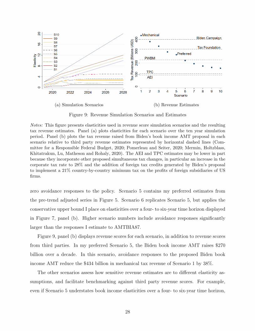
Figure 9 presents ten year revenue scores based on the different response scenarios. Panel

(a) displays the elasticity assumptions in each scenario. The assumed avoidance responses of

firms increase with scenario numbers. Scenario 1 is a mechanical tax calculation that assumes

23Historically, when firms have paid an AMT, they have also generated AMT credits which could beused against normal tax liability in future years. However, the Biden book income AMT proposal does notspecify whether it would include AMT credits. Therefore, I exclude AMT credits from my baseline revenuecalculations, but show back of the envelope adjustments for credits do not materially impact my results.

27

(a) Simulation Scenarios (b) Revenue Estimates

Figure 9: Revenue Simulation Scenarios and Estimates

Notes: This figure presents elasticities used in revenue score simulation scenarios and the resultingtax revenue estimates. Panel (a) plots elasticities for each scenario over the ten year simulationperiod. Panel (b) plots the tax revenue raised from Biden’s book income AMT proposal in eachscenario relative to third party revenue estimates represented by horizontal dashed lines (Com-mittee for a Responsible Federal Budget, 2020; Pomerleau and Seiter, 2020; Mermin, Holtzblass,Khitatrakun, Lu, Matheson and Rohaly, 2020). The AEI and TPC estimates may be lower in partbecause they incorporate other proposed simultaneous tax changes, in particular an increase in thecorporate tax rate to 28% and the addition of foreign tax credits generated by Biden’s proposalto implement a 21% country-by-country minimum tax on the profits of foreign subsidiaries of USfirms.

zero avoidance responses to the policy. Scenario 5 contains my preferred estimates from

the pre-trend adjusted series in Figure 5. Scenario 6 replicates Scenario 5, but applies the

conservative upper bound I place on elasticities over a four- to six-year time horizon displayed

in Figure 7, panel (b). Higher scenario numbers include avoidance responses significantly

larger than the responses I estimate to AMTBIA87.

Figure 9, panel (b) displays revenue scores for each scenario, in addition to revenue scores

from third parties. In my preferred Scenario 5, the Biden book income AMT raises $270

billion over a decade. In this scenario, avoidance responses to the proposed Biden book

income AMT reduce the $434 billion in mechanical tax revenue of Scenario 1 by 38%.

The other scenarios assess how sensitive revenue estimates are to different elasticity as-

sumptions, and facilitate benchmarking against third party revenue scores. For example,

even if Scenario 5 understates book income elasticities over a four- to six-year time horizon,

28

when I apply the conservative upper bound I estimate on these elasticities in Scenario 6, the

Biden book income AMT will still raise $221 billion over a decade.

Matching third party revenue scores with my scoring methodology requires diverging

assumptions about the magnitude of tax avoidance. To achieve a revenue score as high as

the Biden campaign estimate, I have to assume close to zero avoidance response to the policy.

Matching the Tax Policy Center (TPC) or American Enterprise Institute (AEI) estimates

requires additional modifications because they include other concurrently proposed policy

in the Biden tax plan, including an increase in the corporate tax rate to 28% and the

introduction of a 21% country-by-country minimum tax on profits of the foreign subsidiaries

of US firms that could generate additional foreign tax credits. I discuss my procedure

for implementing these scoring modifications in Appendix B, but they only decrease the

revenue raised by the Biden book income AMT in my preferred simulation to $249 billion.

Therefore, even after corporate tax rate and FTC modifications due to a country-by-country

minimum tax, to achieve a revenue score on par with the TPC or AEI estimates I need

to assume avoidance responses more than four times larger than the responses I estimate

to AMTBIA87.24 Wald tests reject the null hypotheses at the 5% level that my baseline

or upper bound elasticity estimates over a three- and six-year time horizon are equal to

the elasticity assumptions in Scenario 2 and Scenario 10, the closest matches to the Biden

campaign and AEI estimates.

I summarize the revenue raised by the proposed Biden book income AMT in each sim-

ulation scenario in Table 3, panel A, and external revenue estimates for the policy by third

parties in panel B. The elasticity assumptions displayed in the table match those displayed in

24TPC or AEI may also calculate lower revenue scores by incorporating the offsetting value of minimumtax credits generated by past AMTs. I ignore minimum tax credits in my analysis because the Biden bookincome AMT proposal does not mention the inclusion of an accompanying minimum tax credit. To evaluatehow large of an impact these credits might have on revenues, I can adjust my revenue scores using a backof the envelope calculation. For example, if firms have a discount rate of 7% and reclaim half of their AMTpayments as minimum tax credits over the ten years following the payments (10% of their yearly paymentin the first, third, fifth, seventh and ninth year following each payment) it would reduce the revenue scoreby 36%. This calculation is consistent with data indicating only 57.1% of all minimum tax credits availablein 1993, but originating back through 1987, were used by 1998, even though minimum tax credit use wasabove its 1988-2002 average in the years between 1993-1998 (Carlson, 2001, 2005). Even after includingthis minimum tax credit adjustment in addition to adjustments for a higher corporate tax rate and FTCsgenerated by a country-by-country minimum tax, the revenue score I estimate in my preferred specificationfar exceeds the revenue estimates from TPC or AEI.

29

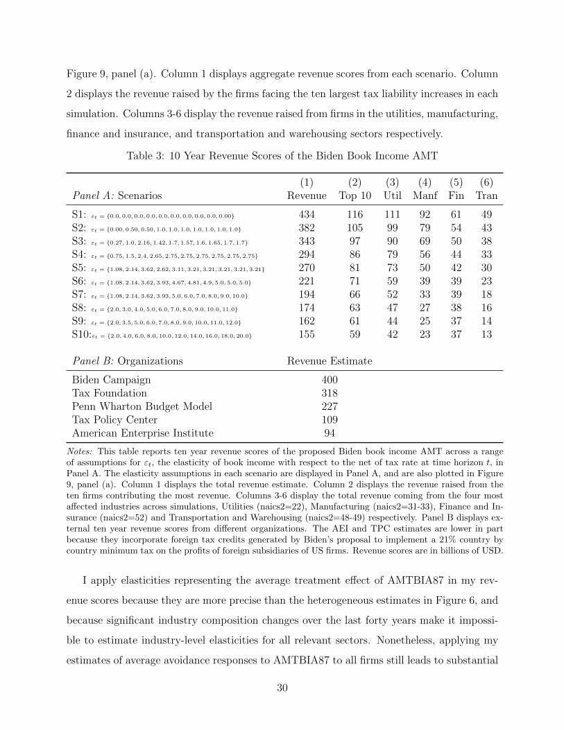
Figure 9, panel (a). Column 1 displays aggregate revenue scores from each scenario. Column

2 displays the revenue raised by the firms facing the ten largest tax liability increases in each

simulation. Columns 3-6 display the revenue raised from firms in the utilities, manufacturing,

finance and insurance, and transportation and warehousing sectors respectively.

Table 3: 10 Year Revenue Scores of the Biden Book Income AMT

(1) (2) (3) (4) (5) (6)Panel A: Scenarios Revenue Top 10 Util Manf Fin Tran

S1: εt = {0.0, 0.0, 0.0, 0.0, 0.0, 0.0, 0.0, 0.0, 0.0, 0.00} 434 116 111 92 61 49S2: εt = {0.00, 0.50, 0.50, 1.0, 1.0, 1.0, 1.0, 1.0, 1.0, 1.0} 382 105 99 79 54 43S3: εt = {0.27, 1.0, 2.16, 1.42, 1.7, 1.57, 1.6, 1.65, 1.7, 1.7} 343 97 90 69 50 38S4: εt = {0.75, 1.5, 2.4, 2.65, 2.75, 2.75, 2.75, 2.75, 2.75, 2.75} 294 86 79 56 44 33S5: εt = {1.08, 2.14, 3.62, 2.62, 3.11, 3.21, 3.21, 3.21, 3.21, 3.21} 270 81 73 50 42 30S6: εt = {1.08, 2.14, 3.62, 3.93, 4.67, 4.81, 4.9, 5.0, 5.0, 5.0} 221 71 59 39 39 23S7: εt = {1.08, 2.14, 3.62, 3.93, 5.0, 6.0, 7.0, 8.0, 9.0, 10.0} 194 66 52 33 39 18S8: εt = {2.0, 3.0, 4.0, 5.0, 6.0, 7.0, 8.0, 9.0, 10.0, 11.0} 174 63 47 27 38 16S9: εt = {2.0, 3.5, 5.0, 6.0, 7.0, 8.0, 9.0, 10.0, 11.0, 12.0} 162 61 44 25 37 14S10:εt = {2.0, 4.0, 6.0, 8.0, 10.0, 12.0, 14.0, 16.0, 18.0, 20.0} 155 59 42 23 37 13

Panel B: Organizations Revenue Estimate

Biden Campaign 400Tax Foundation 318Penn Wharton Budget Model 227Tax Policy Center 109American Enterprise Institute 94

Notes: This table reports ten year revenue scores of the proposed Biden book income AMT across a rangeof assumptions for εt, the elasticity of book income with respect to the net of tax rate at time horizon t, inPanel A. The elasticity assumptions in each scenario are displayed in Panel A, and are also plotted in Figure9, panel (a). Column 1 displays the total revenue estimate. Column 2 displays the revenue raised from theten firms contributing the most revenue. Columns 3-6 display the total revenue coming from the four mostaffected industries across simulations, Utilities (naics2=22), Manufacturing (naics2=31-33), Finance and In-surance (naics2=52) and Transportation and Warehousing (naics2=48-49) respectively. Panel B displays ex-ternal ten year revenue scores from different organizations. The AEI and TPC estimates are lower in partbecause they incorporate foreign tax credits generated by Biden’s proposal to implement a 21% country bycountry minimum tax on the profits of foreign subsidiaries of US firms. Revenue scores are in billions of USD.

I apply elasticities representing the average treatment effect of AMTBIA87 in my rev-

enue scores because they are more precise than the heterogeneous estimates in Figure 6, and

because significant industry composition changes over the last forty years make it impossi-

ble to estimate industry-level elasticities for all relevant sectors. Nonetheless, applying my

estimates of average avoidance responses to AMTBIA87 to all firms still leads to substantial

30

tax burden heterogeneity across firms and industries in revenue simulations. Column 2 of

Table 3 shows that across scenarios, between 27-38% of the revenue raised by the proposed

Biden book income AMT comes from the firms with the ten largest tax liability increases

due to the policy.25 Columns 3-6 of Table 3 show that, across revenue simulations, most of

the revenue raised by the proposed Biden book income AMT would come from the utilities,

manufacturing, finance and insurance and transportation and warehousing sectors.

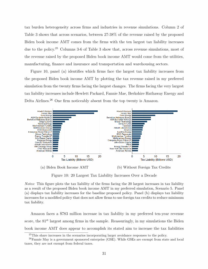
Figure 10, panel (a) identifies which firms face the largest tax liability increases from

the proposed Biden book income AMT by plotting the tax revenue raised in my preferred

simulation from the twenty firms facing the largest changes. The firms facing the very largest

tax liability increases include Hewlett Packard, Fannie Mae, Berkshire Hathaway Energy and

Delta Airlines.26 One firm noticeably absent from the top twenty is Amazon.

(a) Biden Book Income AMT (b) Without Foreign Tax Credits

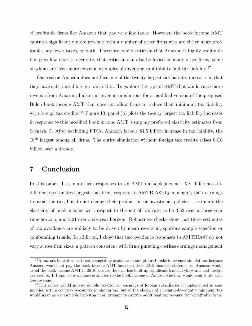
Figure 10: 20 Largest Tax Liability Increases Over a Decade

Notes: This figure plots the tax liability of the firms facing the 20 largest increases in tax liabilityas a result of the proposed Biden book income AMT in my preferred simulation, Scenario 5. Panel(a) displays tax liability increases for the baseline proposed policy. Panel (b) displays tax liabilityincreases for a modified policy that does not allow firms to use foreign tax credits to reduce minimumtax liability.

Amazon faces a $783 million increase in tax liability in my preferred ten-year revenue

score, the 81st largest among firms in the sample. Reassuringly, in my simulations the Biden

book income AMT does appear to accomplish its stated aim to increase the tax liabilities

25This share increases in the scenarios incorporating larger avoidance responses to the policy.26Fannie May is a government sponsored enterprise (GSE). While GSEs are exempt from state and local

taxes, they are not exempt from federal taxes.

31

of profitable firms like Amazon that pay very few taxes. However, the book income AMT

captures significantly more revenue from a number of other firms who are either more prof-

itable, pay fewer taxes, or both. Therefore, while criticism that Amazon is highly profitable

but pays few taxes is accurate, that criticism can also be levied at many other firms, some

of whom are even more extreme examples of diverging profitability and tax liability.27

One reason Amazon does not face one of the twenty largest tax liability increases is that

they have substantial foreign tax credits. To explore the type of AMT that would raise more

revenue from Amazon, I also run revenue simulations for a modified version of the proposed

Biden book income AMT that does not allow firms to reduce their minimum tax liability

with foreign tax credits.28 Figure 10, panel (b) plots the twenty largest tax liability increases

in response to this modified book income AMT, using my preferred elasticity estimates from

Scenario 5. After excluding FTCs, Amazon faces a $4.5 billion increase in tax liability, the

10th largest among all firms. The entire simulation without foreign tax credits raises $316

billion over a decade.

7 Conclusion

In this paper, I estimate firm responses to an AMT on book income. My differences-in-

differences estimates suggest that firms respond to AMTBIA87 by managing their earnings

to avoid the tax, but do not change their production or investment policies. I estimate the

elasticity of book income with respect to the net of tax rate to be 3.62 over a three-year

time horizon, and 3.21 over a six-year horizon. Robustness checks show that these estimates

of tax avoidance are unlikely to be driven by mean reversion, spurious sample selection or

confounding trends. In addition, I show that tax avoidance responses to AMTBIA87 do not

vary across firm sizes, a pattern consistent with firms pursuing costless earnings management

27Amazon’s book income is not changed by avoidance assumptions I make in revenue simulations becauseAmazon would not pay the book income AMT based on their 2018 financial statements. Amazon wouldavoid the book income AMT in 2018 because the firm has built up significant loss carryforwards and foreigntax credits. If I applied avoidance estimates to the book income of Amazon the firm would contribute evenless revenue.

28This policy would impose double taxation on earnings of foreign subsidiaries if implemented in con-junction with a country-by-country minimum tax, but in the absence of a country-by-country minimum taxwould serve as a reasonable backstop in an attempt to capture additional tax revenue from profitable firms.

32

to avoid AMTBIA87 before pursuing costly changes to production or investment.

The purpose of AMTs is to bolster public perceptions of tax code fairness by ensuring all

firms with substantial income pay taxes. To evaluate the implications of the tax avoidance I

estimate in response to AMTBIA87 for contemporary policy, I develop revenue scores of the

proposed Biden book income AMT. In my preferred simulation, the Biden book income AMT

would raise $270 billion in revenue over a decade. These revenue scores make two important

points. First, the Biden book income AMT would raise substantial revenue from firms with

high income and low tax liability, but firms would still have some scope to escape larger tax

payments because of net operating losses and foreign tax credits. Second, benchmarking my

revenue scores against third party estimates reveals that matching third party scores of the

Biden book income AMT requires making assumptions about firm tax avoidance that are

inconsistent with the tax avoidance I estimate in response to AMTBIA87.

This paper considers firm responses to a book income AMT and the implications of

those responses for the effectiveness of contemporary proposals to implement a book income

AMT. However, any policy debate over implementing an AMT based on book income would

be incomplete without also considering possible loss of information content for investors

(Hanlon, Laplant and Shevlin, 2005), dead weight loss associated with a book income tax

(Dharmapala, 2020), politicization of the accounting standards setting process (Shaviro,

2020), and the interaction of a book income AMT with all other business tax incentives.

Ultimately, we have only incomplete historical evidence to guide the implementation of a

tax based on book income, and any implementation of a book income AMT in the future

will call for careful evaluation.

33

References

Alejos, Luis. 2018. “Firms’ (Mis)-Reporting under a Minimum Tax: Evidence fromGuatemalan Corporate Tax Returns.” Working Paper.

Almunia, Miguel, and David Lopez-Rodriguez. 2018. “Under the Radar: The Effectsof Monitoring Firms on Tax Compliance.” American Economic Journal: Economic Policy,10(1): 1–38.

Bachas, Pierre, and Mauricio Soto. Forthcoming. “Corporate Taxation under WeakEnforcement.” American Economic Journal: Economic Policy.

Best, Michael C., Anne Brockmeyer, Henrik J. Kleven, Johannes Spinnewijn,and Mazhar Waseem. 2015. “Production versus Revenue Efficiency with LimitedTax Capacity: Theory and Evidence from Pakistan.” Journal of Political Economy,123(6): 1311–1355.

Blouin, Jennifer, and Leslie Robinson. 2020. “Double counting accounting: How muchprofit of multinational enterprises is really in tax havens?” Working Paper.

Boynton, Charles E., Paul S. Dobbins, and George A. Plesko. 1992. “Earnings Man-agement and the Corporate Alternative Minimum Tax.” Journal of Accounting Research,30: 131–53.

Carlson, Curtis P. 2001. “Who Pays the Corporate Alternative Minimum Tax? Resultsfrom Panel Data for 1987-1998.” Vol. 94, 349–356, Annual Conference on Taxation andMinutes of the Annual Meeting of the National Tax Association.

Carlson, Curtis P. 2005. “The Corporate Alternative Minimum Tax Aggregate HistoricalTrends.” OTA Paper 93.

Choi, Won W., Jeffrey D. Gramlich, and Jacob K. Thomas. 2001. “Potential errorsin detecting earnings management: Reexamining studies investigating the AMT of 1986.”Contemporary Accounting Research, 18(4): 571–613.

Clausing, Kimberly. 2020. “How Big is Profit Shifting?” Working Paper.

Collins, Julie H., and Douglas A. Shackleford. 2004. “Do U.S. Multinationals FaceDifferent Tax Burdens than Do Other Companies?” Tax Policy and the Economy, 17: 141–68.

Committee for a Responsible Federal Budget. 2020. “Understanding Joe Biden’s 2020Tax Plan.” US Budget Watch.

Cooper, Russel W., and John C. Haltiwanger. 2006. “On the Nature of CapitalAdjustment Costs.” Review of Economic Studies, 73: 611–633.

Cummins, Jason G., Kevin A. Hasset, and R. Glenn Hubbard. 1994. “A Reconsid-eration of Investment Behavior Using Tax Reforms as Natural Experiments.” BrookingsPapers on Economic Activity, 24(2): 1–74.

Desai, Mihir A., and Austan D. Gollsbee. 2004. “Investment, Overhang and TaxPolicy.” Brookings Papers on Economic Activity, 34(2): 285–355.

Devereux, Michael P., Li Liu, and Simon Loretz. 2014. “The Elasticity of CorporateTaxable Income: New Evidence from UK Tax Records.” American Economic Journal:Economic Policy, 6(2): 19–53.

34

Dhaliwal, Dan, and Shiing-Wu Wang. 1992. “The effect of book income adjustment inthe 1986 alternative minimum tax on corporate financial reporting.” Journal of Accountingand Economics, 15(1): 7–26.

Dharmapala, Dhammika. 2020. “The Tax Elasticity of Financial Statement Income: Im-plications for Current Reform Proposals.” Working Paper.

Dobkin, Carlos, Amy Finklestein, Raymond Kluender, and Matthew J. No-towidigdo. 2018. “The Economic Consequences of Hospital Admissions.” American Eco-nomic Review, 108(2): 308–352.

Doms, Mark, and Timothy Dunne. 1998. “Capital Adjustment Patterns in Manufac-turing Plants.” Review of Economic Dynamics, 1: 409–429.

Edgerton, Jesse. 2010. “Investment incentives and corporate tax asymmetries.” Journalof Public Economics, 94(11-12): 936–952.

Gaertner, Fabio B., Stacie K. Laplante, and Daniel P. Lynch. 2016. “Trends inthe Sources of Permanent and Temporary Book-Tax Differences During the Schedule M-3Era.” National Tax Journal, 69(4): 785–808.

Gardner, Matthew. 2020. “From 0% to 1.2%: Amazon Lauds Its Minuscule EffectiveFederal Income Tax Rate.” ITEP Just Taxes Blog.

Gerardi, Geraldine, Hudson Milner, and Gerald Silverstein. 1992. “Temporal As-pects of the corporate alternative minimum tax: results from corporate panel data for1987-1990.” Vol. 85, 117–127, Proceedings of the Annual Conference on Taxation Heldunder the Auspices of the National Tax Association-Tax Institute of America.

Gill, Amy, and Patrice Treubert. 1992. “Corporate Alternative Minimum Tax, 1987-1990.” Statistics of Income, Internal Revenue Service. Data Release.

Gramlich, Jeffrey D. 1991. “The effect of the alternative minimum tax book income ad-justment on accrual decisions.” Journal of the American Taxation Association, 12(1): 36–56.

Hanlon, Michelle. 2005. “The Persistence and Pricing of Earnings, Accruals, and CashFlows When Firms Have Large Book-Tax Differences.” The Accounting Review, 80(1): 137–166.

Hanlon, Michelle, Stacie Kelley Laplant, and Terry Shevlin. 2005. “Evidence for thePossible Information Loss of Conforming Book Income and Taxable Income.” The Journalof Law and Economics, 48(2): 407–442.

Janiga, John M. 1988. “The Corporate Alternative Minimum Tax: A Critique and Explo-ration of Alternatives.” Loyola University Chicago Law Journal, 20(1).

Lobel, Felipe, Thiago Scot, and Pedro Zuniga. 2020. “Corporate Taxation and EvasionResponses: Evidence from a Minimum Tax in Honduras.” Working Paper.

Manzon, Gil, and George A. Plesko. 2002. “The relation between financial and taxreporting measures of income.” Tax Law Review, 55: 175–214.

Manzon, Gil B. 1992. “Earnings management of firms subject to the alternative minimumtax.” Journal of the American Taxation Association, 14(2): 88–111.

Mermin, Gordon B., Janet Holtzblass, Surachai Khitatrakun, Chenxi Lu, Thorn-ton Matheson, and Jeffrey Rohaly. 2020. “An Updated Analysis of Former VicePresident Biden’s Tax Proposals.” Tax Policy Center.

35

Mosberger, Palma. 2016. “Accounting versus real production responses among firms totax incentives: bunching evidence from Hungary.” Working Paper.

Ohrn, Eric. 2018. “The Effect of Corporate Taxation on Investment and Financial Policy:Evidence from the DPAD.” American Economic Journal: Economic Policy, 10(2): 272–301.

Pomerleau, Kyle, and Grant M. Seiter. 2020. “An Analysis of Joe Biden’s Tax Pro-posals, October 2020 Update.” American Enterprise Institute.

Rauh, Joshua D., and Jonathan Gruber. 2007. “How Elastic is the Corporate In-come Tax Base?” In Taxing Corporate Income in the 21st Century. , ed. Alan Auerbach,James R. Hines and Joel Slemrod. Cambridge University Press.

Redmond Soneff, Sandra G. 1986. “The Book Income Adjustment in the 1986 TaxReform Act Corporate Minimum Tax: Has Congress Added Needless Complexity in theName of Fairness.” SMU Law Review, 40(5).

Saez, Emmanuel, Joel B. Slemrod, and Seth H. Giertz. 2012. “The Elasticity ofTaxable Income with Respect to Marginal Tax Rates: A Critical Review.” Journal ofEconomic Literature, 50(1): 3–50.

Shaviro, Daniel. 2020. “What Are Minimum Taxes, and Why Might One Favor or DisfavorThem?” Working Paper.

Suarez Serrato, Juan Carlos. 2019. “Unintended Consequences of Eliminating TaxHavens.” Working Paper.

Tørsløv, Thomas, Ludvig Wier, and Gabriel Zucman. 2020. “The Missing Profits ofNations.” Working Paper.

Wang, Shiing-Wu. 1994. “The Relationship between Financial Reporting Practices andthe 1986 Alternative Minimum Tax.” The Accounting Review, 69(3): 495–506.

Wilson, Ryan J. 2009. “An Examination of Corporate Tax Shelter Participants.” TheAccounting Review, 84(3): 969–999.

Zwick, Eric, and James Mahon. 2017. “Tax Policy and Heterogeneous Investment Be-havior.” American Economic Review, 107(1): 217–248.

36

A Relating Effective Tax Rates to AMT Liabilities

I relate effective tax rates to alternative minimum tax book income adjustment (AMTBIA87)

payments building on derivations in Dhaliwal and Wang (1992). First, I define the book

income adjustment (BIA) and alternative minimum tax payments (AMT) under AMTBIA87,

with statutory corporate tax rate τ , taxable income TI, book income BI and tax preferences

and adjustments TPA:

BIA = 0.5(BI − (TI + TPA)

),

AMT = max{

0.2(TI + TPA+BIA

)− τTI, 0

}.

Next, I define book tax differences BTD ≡ BI −TI. AMTBIA87 is a direct tax on BTD−

TPA, the portion of book tax differences that are not tax preferences and adjustments.

Suppose some fraction f of BTD are TPA, so that TPA = f(BI − TI). Then plugging the

expressions for BIA and TPA into AMT , I obtain

AMT

BI= max{0.1 + 0.1f +

[(0.1− τ)− 0.1f

]TIBI

, 0}.

Furthermore, because ETR ≡ τ TIBI

, I can write

AMT

BI= max{0.1 + 0.1f −

[τ − 0.1

τ+

0.1f

τ

]ETR, 0}.

Therefore, a firm has positive AMT liability if

ETR <0.1 + 0.1f(τ−0.1)+0.1f

τ

.

Now suppose f = 0, so that there are no tax preferences and adjustments and AMTBIA87

is a direct tax on BTD. Then a firm faces positive AMT liability if ETR < 0.2. In 1987

τ = 0.4, implying that to obtain an ETR of 0.2, a firm must have BI twice as large as TI.

In 1986, when τ = 0.46, a firm with BI twice as large as TI has an ETR of 0.23. Therefore,

all firms with ETR < 0.23 in 1986 are likely to face positive AMT liability from AMTBIA87.

37

On the other hand, suppose f = 0.5, so that half of BTD are tax preferences and

adjustments and AMTBIA87 is a direct tax on only half of BTD. Then, a firm has positive

AMT liability if ETR < 0.15(0.4−0.05)

0.4

= 0.17 in 1987. To obtain an ETR of 0.17 in 1987, a firm

must have BI 2.33 times as large as TI, while in 1986 a firm must have an ETR of 0.20 to

have BI 2.33 times as large as TI.

Aggregate data released by the IRS suggests that the TPA included in BTD are unlikely

to lead to spurious results. Gill and Treubert (1992) indicates that, averaging across 1987-

1989, f = 0.39, and depreciation of property placed in service after 1986 and depletion

account for 88% of those tax preferences and adjustments. To be conservative, in my baseline

specifications I choose an ETR cutoff of 23% to ensure a high probability that firms in the

control group do not face positive tax liability from AMTBIA87, and include time varying

controls for depreciation and depletion to eliminate variation in the outcome due to TPA

changes. In robustness checks I also find that my results are not sensitive to modifying the

ETR cutoff to 20% or 26%.

B Revenue Scoring Methodology

To develop a revenue score of the Biden book income AMT I simulate the evolution of a

2018 cross section of firm’s book incomes over the scoring time frame while incorporating

avoidance responses to the policy. To select a cross section of firms in 2018, I restrict the

Compustat fundamentals annual data to firms with positive, non-missing assets, sales, and

pretax income that are incorporated in the United States and exist in the data in both 2017

and 2018. I display summary stats for this sample of firms in Table C.1. Relative to the

historical sample, firms are significantly larger in 2018 but exhibit the same type of skew

with means of most variables exceeding medians by a large amount.

In the 2018 cross section of firms, I construct measures of total tax liability, eligible car-

ryforwards for net operating loss deductions, the tax amount potentially due because of the

book income AMT, and new tax due under the book income AMT. I measure applicable tax

loss carryforwards as the minimum of Compustat pretax income and tax loss carryforwards.

I calculate potential tax due because of the book income AMT as 15% of the difference

38

between Compustat pretax income and applicable tax carryforwards, all less foreign taxes.

Finally, I calculate the firm’s new tax liability as the maximum of the firm’s old tax liability

or the potential tax due because of the book income AMT, only applying the AMT if the

firm has over $100 million in EBITD. Summing across the new tax liabilities for firms in the

2018 cross section yields a one year mechanical tax revenue estimate of $38 billion.

To ensure my construction of tax status in the Compustat data is consistent with tax data,

I compare aggregates of tax variables available in SOI line item reports to aggregate proxies

in the Compustat data in Figure C.1 for available years spanning 2008-2015. While there

are differences in aggregates in Compustat and the SOI line item reports, the magnitudes

reasonably track each other across years.

Building on the 2018 cross section, I construct a panel by simulating ten years forward

for each firm, taking into account possible avoidance responses to the proposed Biden book

income AMT. To facilitate a direct mapping from the DiD estimates of avoidance in section

4 into the simulated data, I use CBO’s 2018 ten-year GDP forecast as a proxy for book

income growth per year for all firms, inflating book income (as well as EBITD and all other

tax variables) by the CBO projected growth rate, and calculating book income as the sum

of projected book income and a possible avoidance response to the policy.29

To incorporate firm avoidance responses into the book income projection, I define book

income for each firm in the simulation as the sum of projected mechanical book income, and

a possible avoidance response to the proposed Biden book income AMT,

BIt = BImecht + εt ·BImecht · ∆(1− τ)

1− τ· 1(T = 1), (B.1)

where BImecht is projected book income over the ten-year window applying only CBO GDP

forecasts to 2018 book income, εt is the elasticity of book income with respect to the net

of tax rate over time horizon t that I estimate in section 4, and ∆(1−τ)1−τ = 0.85−1

1= −0.15 is

29To account reasonably for firm losses, I calculate the share of firms with positive losses in 2018 andcalculate the ratio of those firm’s losses to their pretax income. In each subsequent simulation year I randomlyselect a fraction of firms that matches the share with positive losses in 2018, and within this sample subtractthe fraction of pretax income that was removed via applicable losses in the 2018 calculation. In unreportedresults, I find that revenue estimates are similar when I instead calculate the observed fraction of tax losscarryforwards over book income in 2018, and reduce projected book income for every firm by that samefraction in each subsequent simulated year.

39

the change in the net of tax rate after the introduction of the proposed Biden book income

AMT 15% marginal tax on book income.

I capture avoidance responses to the proposed Biden book income AMT with εt ·BImecht ·∆(1−τ)

1−τ · 1(T = 1). The first terms εt · BImecht · ∆(1−τ)1−τ unwind the elasticity into a change

in book income for each firm. 1(T = 1) is an indicator for firms with over $100 million

in EBITD in 2018 that would pay the proposed Biden book income AMT in 2018. This

ensures that I only apply avoidance responses in the revenue simulation to a group of firms

analogous to the treatment group in the DiD in section 4.

The methodology described above calculates a revenue score for Biden’s proposed book

income AMT holding all other tax policies fixed. However, the American Enterprise Institute

(AEI) and Tax Policy Center (TPC) scores of the Biden book income AMT include other

proposed policies in the 2020 Biden tax plan. The most important of these policies for a

revenue score of the Biden book income AMT are an increase in the corporate tax rate to

28%, and a 21% global country-by-country minimum tax on the profits of foreign subsidiaries

of US firms that may generate additional foreign tax credits (FTCs).

To quantify the impacts of these additional policies on revenue raised by the Biden book

income AMT, I modify the revenue scoring procedure outlined above. First, to adjust for

the higher corporate tax rate, I increase all positive tax liabilities in revenue simulations

by 43· (0.985), representing the increase in the corporate tax rate from 21% to 28%, and

incorporating an elasticity of corporate taxable income of 0.15, at the lower end of the range

of existing estimates (Rauh and Gruber, 2007; Devereux, Liu and Loretz, 2014).30 This

adjustment changes scores of the Biden book income AMT because AMT liabilities must

exceed normal tax liabilities for firms to face the AMT.

Second, I adjust for FTCs from a new country-by-country global minimum tax on the

profits of foreign subsidiaries of US firms. Compustat data aggregates to the parent company

level, and therefore does not provide a country-by-country breakdown of income and taxes,

but does provide measures of foreign income and taxes paid. Blouin and Robinson (2020)

argues that Compustat foreign income and tax payments are reasonable measures of the

30This is likely an underestimate of the elasticity because larger firms more likely to be subject to thebook income AMT may have substantially higher elasticities. Devereux, Liu and Loretz (2014) discuss thispoint in more detail.

40

economic activity of foreign subsidiaries of US firms because they do not suffer from double

counting issues and align closely with measures of income and taxes in BEA data. Therefore,

as a rough check of the additional FTCs a 21% global country-by-country minimum tax may

raise, I replace foreign tax payments for all firms in the Compustat data with the maximum

of their foreign tax payments or 21% of their foreign income. Foreign income is often missing

in the Compustat data, which could reflect zero foreign income or a reporting issue. To be

conservative, I impute 2018 foreign income with previous foreign income dating back to 2015

if the data is missing in 2018 (inflating foreign income by 3% per year).31

Adjusting for both a higher corporate tax rate and additional FTCs generated by a

country-by-country global minimum tax yields a revenue estimate of $249 billion, while only

adjusting for FTCs generated by a country-by-country global minimum tax yields a revenue

score of $260 billion. Even with an additional adjustment for possible AMT credits (see

footnote 23), this revenue estimate substanially exceeds the AEI or TPC revenue scores.

However, I wish to stress that the FTC adjustment is a fundamentally uncertain pro-

cedure. The impacts of a global country-by-country minimum tax depend on how much

income multinational firms locate in tax havens, how firms reallocate factors of production

across nations in response to new minimum taxes, and the ability of the new tax to capture

shifted profits, all of which are uncertain parameters and the topic of current debate in the

literature.32 The FTC adjustment may be too conservative because it does not adjust taxes

on a country-by-country basis, and because the financial accounting data in Compustat may

fail to capture substantial amounts of income located in tax havens (Tørsløv, Wier and

Zucman, 2020; Clausing, 2020). The FTC adjustment could also overstate the amount of

FTCs generated because it assumes the new country-by-country minimum tax will be able

to capture all foreign income present in Compustat in the tax base. In addition, any upward

adjustment to my procedure that attempts to account for tax haven income missing from

Compustat would depend on the magnitude of shifted profits, and the share of those shifted

profits that will be captured in the tax base of the country-by-country minimum tax. Ulti-

31I also impute missing foreign tax payments with a $0 foreign tax bill, providing a conservative upperbound on how much tax payments could increase in response to a global country-by-country minimum tax.

32Blouin and Robinson (2020), Clausing (2020) and Tørsløv, Wier and Zucman (2020) are a few recentexamples of the debate over profit shifting. Suarez Serrato (2019) explores how multinationals modify theirfactors of production in response to tax changes.

41

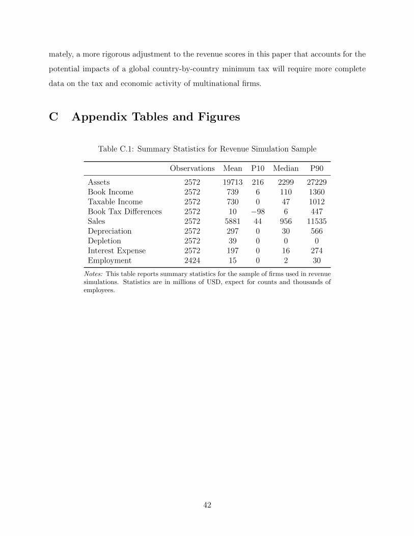
mately, a more rigorous adjustment to the revenue scores in this paper that accounts for the

potential impacts of a global country-by-country minimum tax will require more complete

data on the tax and economic activity of multinational firms.

C Appendix Tables and Figures

Table C.1: Summary Statistics for Revenue Simulation Sample

Observations Mean P10 Median P90

Assets 2572 19713 216 2299 27229Book Income 2572 739 6 110 1360Taxable Income 2572 730 0 47 1012Book Tax Differences 2572 10 −98 6 447Sales 2572 5881 44 956 11535Depreciation 2572 297 0 30 566Depletion 2572 39 0 0 0Interest Expense 2572 197 0 16 274Employment 2424 15 0 2 30

Notes: This table reports summary statistics for the sample of firms used in revenuesimulations. Statistics are in millions of USD, expect for counts and thousands ofemployees.

42

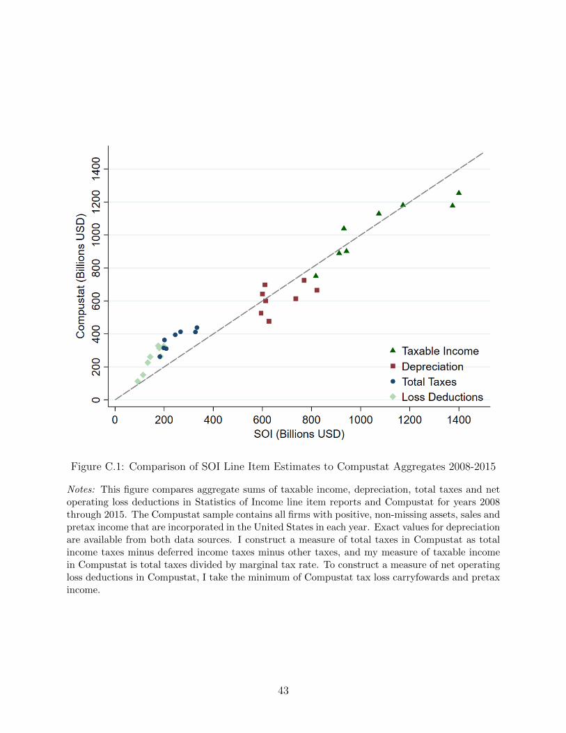
Figure C.1: Comparison of SOI Line Item Estimates to Compustat Aggregates 2008-2015

Notes: This figure compares aggregate sums of taxable income, depreciation, total taxes and netoperating loss deductions in Statistics of Income line item reports and Compustat for years 2008through 2015. The Compustat sample contains all firms with positive, non-missing assets, sales andpretax income that are incorporated in the United States in each year. Exact values for depreciationare available from both data sources. I construct a measure of total taxes in Compustat as totalincome taxes minus deferred income taxes minus other taxes, and my measure of taxable incomein Compustat is total taxes divided by marginal tax rate. To construct a measure of net operatingloss deductions in Compustat, I take the minimum of Compustat tax loss carryfowards and pretaxincome.

43